
Evaluation of Eight Global Precipitation Datasets in Hydrological Modeling


1
Institute of Heavy Rain, China Meteorological Administration (CMA), Wuhan 430205, China
2
State Key Laboratory of Water Resources and Hydropower Engineering Science, Wuhan University, Wuhan 430072, China
3
NORCE Norwegian Research Centre, Bjerknes Centre for Climate Research, Jahnebakken 5, NO-5007 Bergen, Norway
*
Author to whom correspondence should be addressed.
Remote Sens. 2021, 13(14), 2831; https://0-doi-org.brum.beds.ac.uk/10.3390/rs13142831
Submission received: 2 June 2021
/
Revised: 14 July 2021
/
Accepted: 14 July 2021
/
Published: 19 July 2021
(This article belongs to the Topic High-Resolution Earth Observation Systems, Technologies, and Applications)
Abstract
:The number of global precipitation datasets (PPs) is on the rise and they are commonly used for hydrological applications. A comprehensive evaluation on their performance in hydrological modeling is required to improve their performance. This study comprehensively evaluates the performance of eight widely used PPs in hydrological modeling by comparing with gauge-observed precipitation for a large number of catchments. These PPs include the Global Precipitation Climatology Centre (GPCC), Climate Hazards Group Infrared Precipitation with Station dataset (CHIRPS) V2.0, Climate Prediction Center Morphing Gauge Blended dataset (CMORPH BLD), Precipitation Estimation from Remotely Sensed Information using Artificial Neural Networks Climate Data Record (PERSIANN CDR), Tropical Rainfall Measuring Mission multi-satellite Precipitation Analysis 3B42RT (TMPA 3B42RT), Multi-Source Weighted-Ensemble Precipitation (MSWEP V2.0), European Center for Medium-range Weather Forecast Reanalysis 5 (ERA5) and WATCH Forcing Data methodology applied to ERA-Interim Data (WFDEI). Specifically, the evaluation is conducted over 1382 catchments in China, Europe and North America for the 1998-2015 period at a daily temporal scale. The reliabilities of PPs in hydrological modeling are evaluated with a calibrated hydrological model using rain gauge observations. The effectiveness of PPs-specific calibration and bias correction in hydrological modeling performances are also investigated for all PPs. The results show that: (1) compared with the rain gauge observations, GPCC provides the best performance overall, followed by MSWEP V2.0; (2) among the eight PPs, the ones incorporating daily gauge data (MSWEP V2.0 and CMORPH BLD) provide superior hydrological performance, followed by those incorporating 5-day (CHIRPS V2.0) and monthly (TMPA 3B42RT, WFDEI, and PERSIANN CDR) gauge data. MSWEP V2.0 and CMORPH BLD perform better than GPCC, underscoring the effectiveness of merging multiple satellite and reanalysis datasets; (3) regionally, all PPs exhibit better performances in temperate regions than in arid or topographically complex mountainous regions; and (4) PPs-specific calibration and bias correction both can improve the streamflow simulations for all eight PPs in terms of the Nash and Sutcliffe efficiency and the absolute bias. This study provides insights on the reliabilities of PPs in hydrological modeling and the approaches to improve their performance, which is expected to provide a reference for the applications of global precipitation datasets.
1. Introduction
Precipitation is closely related to atmospheric circulation and is a critical component of hydrological cycle [1,2,3]. Accurate precipitation records are not only essential for meteorological and climatic analysis but also the keys for successful water resource management [4,5]. However, acquiring reliable and consistent precipitation series is a challenging task throughout the world. The advent of global precipitation datasets (PPs) including gauge-based, satellite-related, and reanalysis datasets, brings an unprecedented opportunity for precipitation estimation and hydrological application.
However, these PPs differ in design objective, data sources, spatial resolution, spatial coverage, temporal resolution, temporal span, and latency. Consequently, evaluations have been carried out to understand the respective advantages and limitations of PPs [6,7].
There has been a plethora of literature addressing the evaluation of PPs through ground truthing, referring to comparing PPs against rain gauge observations [8,9,10,11] or gauge-adjusted radar fields [12,13]. For example, Bosilovich and Chen [14] evaluated the strengths and weakness of five reanalysis precipitation datasets, compared with two observed datasets. They found that the National Centers for Environmental Prediction–National Center for Atmospheric Research (NCEP–NCAR) reanalysis [15], and the Hadley circulation in the 40-yr European Centre for Medium-Range Weather Forecasts (ECMWF) reanalysis (ERA-40) [16] could, respectively, well capture spatial patterns of observed precipitation in some ocean regions and Northern Hemisphere continents. In addition, the Japanese 25-year reanalysis (JRA-25) [17] showed good performances in the Northern Hemisphere continents and the tropical oceans but contained distinct variation according to the available observing systems. In addition, Beck and Pan [18] evaluated 26 daily precipitation datasets using Stage-IV gauge-radar data across the CONUS for the 2008–2017 period. They found that Multi-Source Weighted-Ensemble Precipitation (MSWEP) V2.2 [19] and European Centre for ECMWF Reanalysis 5 High Resolution (ERA5-HRES) [20], respectively, showed better performances among the 11 gauge-corrected datasets and the 15 uncorrected datasets.
Further, the hydrological evaluation of PPs by assessing their capabilities to reproduce the observed streamflow continues to gain popularity amongst researchers [21,22,23]. For example, Li and Chen [24] analyzed the hydrological utility of the Integrated Multi-satellite Retrievals for Global Precipitation Measurement (GPM IMERG) [25] precipitation datasets in a mountainous region in southern China based on a semi-distributed hydrological model. Their results showed the potential of the IMERG dataset for hydrological modeling in tropical mountain watersheds where information is scarce. In addition, Beck and Vergopolan [26] evaluated nine gauge-corrected PPs in hydrological modeling by calibrating a conceptual hydrological model against streamflow records from 9053 catchments worldwide, and found that the PPs incorporating daily gauge data generally provided better calibrating scores, while the good performance was unlikely to translate to sparsely or ungauged regions.
However, among the hydrological applications of PPs that have been conducted recently, most show an equal or inferior performance compared with those using rain gauge observations [26,27,28]. This might be due to the precipitation errors that exist in PPs, which could be amplified or dampened in hydrological modeling [29,30]. Therefore, researchers usually impose a bias correction of PPs to reduce the precipitation bias, or specifically calibrate the hydrologic model to each PPs (PPs-specific calibration) against observed streamflow to overcome the precipitation bias through the calibration process. For instance, Hughes [31] reported a preliminary analysis of the potential for hydrological modeling using satellite-related precipitation estimates over four catchments in the southern Africa region. They found that the satellite data could not reflect the strong influences on precipitation of topography in some of the catchments unless adjustments were applied to it. In the study over four catchments in Italy, Ciabatta and Brocca [32] found that the Tropical Rainfall Measurement Mission (TRMM) Multi-satellite Precipitation Analysis (TMPA) [33] 3B42RT dataset could improve the performance of a simple hydrological model after bias correction. Behrangi and Khakbaz [21] conducted a hydrological modeling using five satellite-based precipitation datasets in a mid-size catchment in South US, and found that the streamflow pattern could be well captured at both 6 h and monthly time scales when employing PPs-specific calibration.
According to previous studies, the general finding is that there exist large uncertainties in PPs and hydrological applications driving with different PPs, highlighting the importance of evaluation and improvement of which for research and operational applications alike. However, most of these studies evaluated only a subset of the available PPs, either focused on satellite [27,34,35] or reanalysis [14,36,37] within limited regions and time periods [21,35,38], leading to a lack of comprehensive results. Although Beck and Vergopolan [26] evaluated nine global precipitation datasets in hydrological modeling over 9053 catchments worldwide and generated comprehensive results to a certain extent, they did not include the bias correction approach which had been widely used to improve hydrological performances. What is more, although there have been many studies applying the PPs-specific calibration or bias correction method when using PPs for hydrological modeling, few studies focus on the comparison between these two approaches.
Therefore, this study focuses on the evaluation of eight widely used PPs (see Table 1 for overview) during the 1998–2015 period at a daily temporal scale. The specific objectives of this study are: (1) to evaluate the eight PPs by comparing with gauge-observed precipitation over 1382 catchments; (2) to evaluate the reliabilities of PPs for hydrological modeling with calibrated hydrological model using rain gauge observations; and (3) to investigate the effectiveness of bias correction and PPs-specific calibration in hydrological modeling performances. The ultimate goal of this study is to put insight on the reliabilities of PPs as well as their performances in hydrological modeling.
2. Datasets
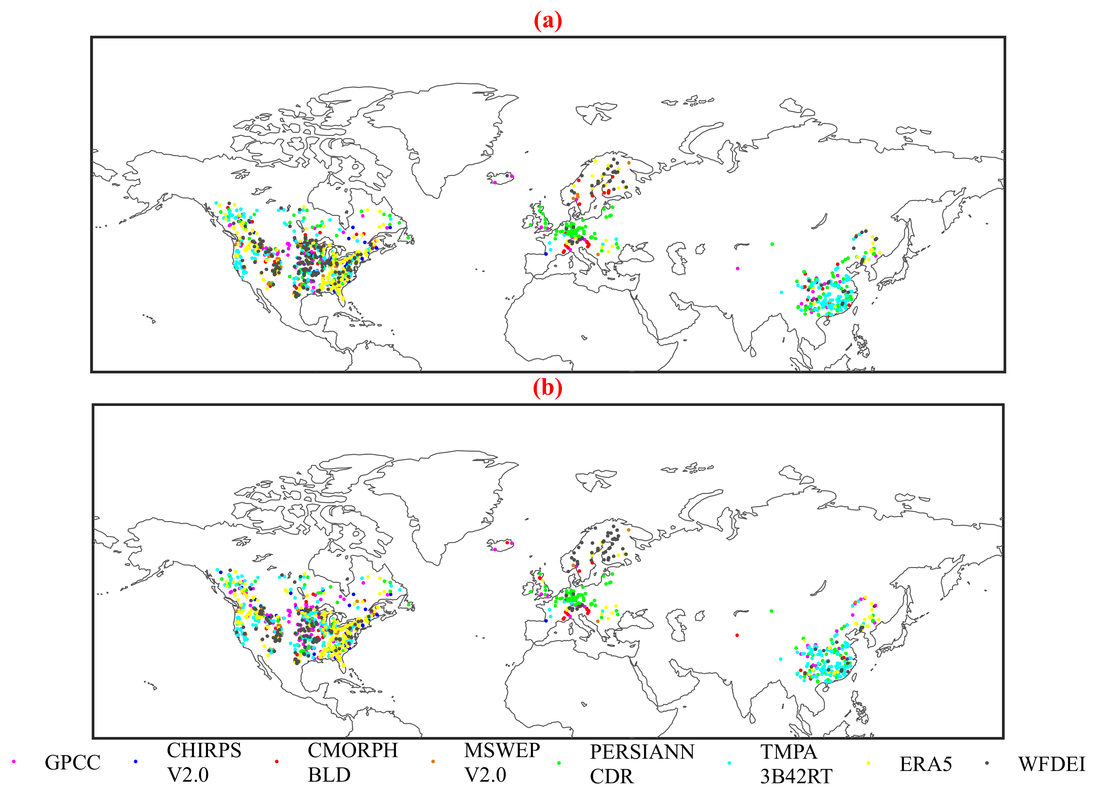
Table 1 presents all datasets used in this study, including the eight PPs for precipitation evaluation and the other meteorological datasets for hydrological modeling, i.e., gauge-observed precipitation, temperature and the gridded potential evaporation data, as well as the daily streamflow data used for hydrological model calibration. In this study, all the gridded datasets were interpolated to catchment-averaged values by using the Thiessen Polygon method [39] for hydrological modeling. The interpolation was executed on a daily time step for the 17-year time period (1998–2015). Considering the data quality and availability of ground observations, the evaluation was carried out over 1382 catchments in China, Europe and North America.
2.1. Global Precipitation Datasets
There are eight PPs evaluated in this study, including one gauge-based dataset: Global Precipitation Climatology Centre (GPCC); five satellite-related datasets: Climate Hazards Group Infrared Precipitation with Station dataset (CHIRPS) V2.0, Climate Prediction Center Morphing (CMORPH) Gauge Blended dataset (CMORPH BLD), Precipitation Estimation from Remotely Sensed Information using Artificial Neural Networks (PERSIANN) Climate Data Record (PERSIANN CDR), TMPA 3B42RT, and MSWEP V2.0; and two reanalysis datasets: ERA5, and WATCH Forcing Data methodology (WFD) applied to ERA-Interim Data (WFDEI). The evaluation was conducted during the common period of the eight PPs, which was 1998–2015.
GPCC is the largest gauge-based dataset, and was developed to collect, perform quality control on, and analyze rain gauge data across the globe.
Satellite-related datasets use polar-orbiting passive microwave (PMW) sensors on low-Earth-orbiting satellites and geosynchronous infrared (IR) sensors on geostationary satellites to estimate precipitation [4,6], and usually blend rain gauge data to offset their limited abilities [50]. In specific, PERSIANN CDR and TMPA 3B42RT mainly respectively applied IR data and PMW data, while the other three integrated both IR and PMW data. MSWEP V2.0 and CMORPH BLD directly incorporated daily gauge data, CHIRPS V2.0 incorporated 5-day gauge data, and TMPA 3B42RT and PERSIANN CDR incorporated monthly gauge data.
Reanalysis-based datasets are designed to generate various meteorological variables with a consistent spatial and temporal resolution by assimilating observations such as weather stations, satellites, ships, and buoys based on different climate models. ERA5 is the fifth generation of atmospheric reanalysis data to replace ERA-Interim produced by ECMWF, assimilating observations from over 200 satellite instruments or types of conventional data and information on rain rate from ground-based radar-gauge composite observations. WFDEI was generated by applying WFD to the ERA-Interim reanalysis data, and used the monthly GPCC in bias correction.
2.2. Other Meteorological Datasets
In the study, we used the gauge-observed precipitation to evaluate the PPs, as well as to calibrate the hydrological model together with the observed temperature. More specifically, we used the gauge-observed precipitation and temperature in China, which came from the China Ground Rainfall/temperature Daily Value 0.5° × 0.5° Lattice Dataset (CGRD/CGTD) (http://data.cma.cn, accessed on 16 July 2021). The CGRD/CGTD was generated by interpolating daily observed precipitation/temperature from more than 2000 meteorological stations in China, the reliability of which has been proved by Zhao and Zhu [51]. In addition, the gauge-observed precipitation and temperature used in Europe were the E-OBS [45], which was a European high-resolution gridded dataset derived from the Europe Climate Assessment & Dataset (ECA&D). The ECA&D forms the strong backbone of the E-OBS since it collects 66865 series of observations at 19087 meteorological stations throughout Europe. Furthermore, the observations used in North America were from a combination of Canadian and United States databases. For Canada, hydrometeorological data and boundary data were from the Canadian model parameter experiment (CANOPEX) database [46]. For US, precipitation and temperature were from the Santa Clara database [47] and streamflow and boundary data were from the United States Geological Survey (USGS) database [49]. Those observed precipitation and temperature data were catchment averaged.
The Global Land Evaporation Amsterdam Model (GLEAM) is a set of algorithms estimating different components of land evaporation [52], whose gridded potential evaporation data was used as an input of the hydrological model for hydrological modeling in this study. The reliability of GLEAM has been tested by Martens and Miralles [48].
2.3. Observed Streamflow
The observed streamflow and boundary data for Chinese catchments were collected from different streamflow-gauging stations. For Europe, they came from the most complete in-situ discharge dataset freely available to the global scientific community, the Global Runoff Data Center (GRDC) dataset (http://grdc.bafg.de, accessed on 16 July 2021). The GRDC is known as the most accurately measured component of the water cycle since it is dedicated to collecting and archiving river discharge data globally [53]. For North America, the observed streamflow and boundary data were from the CANOPEX database and the USGS database mentioned above.
The following two criteria were used to select suitable catchments for hydrological modeling: (1) the catchment area is >2500 km2 and <50,000 km2. The former is to prevent catchments unrepresentative of the 0.5° grid cells (2500 km2 at 0° latitude) from confounding the results and the latter is to reduce the error of catchment averaged values extracted from gridded datasets. (2) The time series of streamflow has to be ≥5 years (can be intermittent) during 1998–2015. Therefore, 232, 184 and 966 catchments were selected from China, Europe and North America, respectively.
3. Methods
The workflow of this study is illustrated below, and more details of the hydrological model (Xin’anjiang (XAJ) model) and the methods applied for evaluation of PPs are described in Section 3.1, Section 3.2 and Section 3.3.
- (1)
- PPs evaluation was conducted by comparison with the rain gauge observations over the selected catchments. In addition, we applied a bias correction method to PPs and obtained “bias corrected-PPs” (BC-PPs), which were also conducted in the comparison.
- (2)
- The hydrological model calibration was firstly performed driven by rain gauge observations, and the calibrated parameter set was referred to as the ‘‘Reference Parameter-sets’’ (RP). The performance of hydrological model calibration served as a benchmark value for later hydrological modeling driving by the eight PPs.
- (3)
- The performances of hydrological modeling with the PPs were evaluated in the following three steps: in step 1, the reliability of PPs for hydrological modeling was investigated by running the model with RP in the calibration period; in step 2, a hydrological model was calibrated by each PPs, which was called PPs-specific calibration, and then their performances were compared with the benchmark value; in step 3, the BC-PPs were used to drive the hydrological model based on the RP in the calibration period and their performances were compared with the benchmark value.
3.1. XAJ Model
The XAJ model [54] is a conceptual rainfall-runoff model which has been widely used in China and many other countries for streamflow simulations [55,56,57]. Figure 1 shows the flowchart of this deterministic lumped model. The calculation process of the XAJ consists of four parts: the evaporation module, the runoff yielding module, the runoff sources partition module, and the runoff concentration module. The evaporation is calculated in three soil layers, including an upper layer, a lower layer and a deep layer, based on the watershed saturation-excess runoff theory. The storage curve calculates the total runoff based on the concept of runoff formation on repletion of storage, which means that runoff is not generated until soil moisture reaches the filled capacity. By using a free water capacity distribution curve, the total runoff is divided into three components including surface runoff, interflow and groundwater runoff. The surface runoff is routed by the unit hydrograph, the interflow and groundwater flow are routed by the linear reservoir method. There are 15 parameters within the XAJ model, four accounting for evaporation, two accounting for runoff generation and nine accounting for runoff routing. More details can be found in Zhao [54]. In addition, the CemaNeige module is added to the XAJ model to simulate the snow accumulation and snowmelt processes since the lack of a snow component in XAJ limits its applicability in snow-dominated watersheds. The CemaNeige module separates precipitation into rainfall and snowfall and calculates the snowmelt based on a degree-day method, which has two parameters to be calibrated [58]. Overall, the XAJ model used in this study contains 17 parameters.
XAJ requires catchment averaged precipitation, temperature and potential evaporation as inputs. For each catchment, the XAJ model was calibrated by the first 70% of observed streamflow data (using the first year as warm-up) and validated by the last 30%. The calibration was performed using the SCE-UA algorithm [59] to optimize model parameter-sets based on the objective function of the Nash and Sutcliffe efficiency (NSE) [60].
3.2. Bias Correction Method
A distribution-based bias correction method called the Daily Bias Correction (DBC) method [61] was applied to correct the catchment averaged precipitation for each PPs in the study. The DBC is a hybrid method combining the Local Intensity Scaling (LOCI) method [62] to correct the precipitation occurrence and the Daily Translation (DT) method [63] to correct the frequency distribution of precipitation. Here are the two steps of the DBC method used in this study:
- (1).
- The LOCI method was used to correct the precipitation occurrence, which ensured that the frequency of the precipitation occurrence estimated by PPs equaled to that of the observed data for a specific month.
- (2).
- The DT method was then used to correct the empirical distribution of PPs-estimated precipitation magnitudes in terms of 100 quantiles from 0.01 to 1 with an interval of 0.01.
3.3. Performance Evaluation Indices
The evaluation of PPs was conducted using the gauge-observed precipitation over the selected catchments based on three statistical indices as follows:
- (1)
- The Pearson linear correlation coefficient (R) is used to assess the agreement between 3-day means of PPs and gauge-observed precipitation as follows:where and are the 3-day mean PPs and gauge-observed precipitation time series, respectively. and are the average of all the 3-day means of PPs and gauge-observed precipitation, respectively. is the length of 3-day mean time series. The R ranges from − to 1 and a larger R represents a better performance. Note that the R is calculated for 3-day mean rather than daily precipitation estimates, as Beck and Vergopolan [26] did, which is done to reduce the impact of the issue with gauge reporting times (i.e., the start and end times of the daily accumulations).
- (2)
- The relative bias ratio (RB) is used to assess the systematic bias of precipitation estimates of PPs and it is also used to assess the systematic bias of the simulated discharge as follows:where and are the daily values of the ith day for the gauge-observed precipitation and the PPs, respectively. and are the average of all the daily values for the gauge-observed precipitation and the PPs, respectively. is the number of days. The RB ranges from - to and the best result is 0.
- (3)
- The root mean square error (RMSE) is used to assess the difference between PPs and gauge-observed precipitation as follows:The RMSE ranges from 0 to and a smaller RMSE represents a better performance.
The hydrological performances of PPs are evaluated by calculating NSE index between the observed and simulated discharge. The NSE is shown as follows:
where and are the daily values of the ith day for the observed and simulated streamflow, respectively. is the average of all the daily values for the observedstreamflow. The NSE ranges from − to 1 and a larger NSE represents a better performance.
4. Results and Discussion
4.1. Evaluation of Precipitation Estimates
In this Section, the PPs and BC-PPs are compared with the gauge-observed precipitation over 1382 catchments for the 1998-2015 period. Figure 2 presents the performances in terms of the R calculated for 3-day means (R3day), RB and RMSE. It shows that GPCC is superior to other PPs in terms of both R3day (median: 0.83) and RMSE (median: 4.54), and the absolute RB (median: 2.40) which is only larger than that of MSWEP V2.0 (median: 0.81). The good performance of GPCC is in line with the study of Schneider, Becker [64], and is attributed to it is the largest gauge-based dataset, with data collected from more than 70,000 different stations worldwide [40]. Note that the use of R3day can only reduce but cannot completely eliminate the impact of reporting time issues. Therefore, it is possible that the good performance of GPCC is also attributed to the similar time shifts between the reference observations and GPCC. The MSWEP V2.0 appears to perform better than the remaining six PPs in terms of the median value of three indices (R3day of 0.82, absolute RB of 0.81, RMSE of 5.21), underscoring the effectiveness of merging multiple satellite and reanalysis datasets, which is in agreement with the finding of Beck and Vergopolan [26]. The ERA5 performs well in terms of R3day (median: 0.80) and RMSE (median: 4.92) but attains the worst absolute RB (median: 7.89). The larger relative biases in precipitation estimates from ERA5 are inconsistent with the findings of Jiang and Li [65]. The MSWEP V2.0, GPCC and CHIRPS V2.0 attain better RB scores, which are attributed to the use of gauge-based Climate Hazards Center’s Precipitation Climatology (CHPclim) dataset [66] or Global Climate Data (WorldClim) [67] to determine their long-term mean. The median scores of R3day, absolute RB and RMSE for the eight BC-PPs are 0.67~0.83, 0.07~3.12, and 4.84~5.63, respectively, which shows generally better performance than that from the eight raw-PPs.
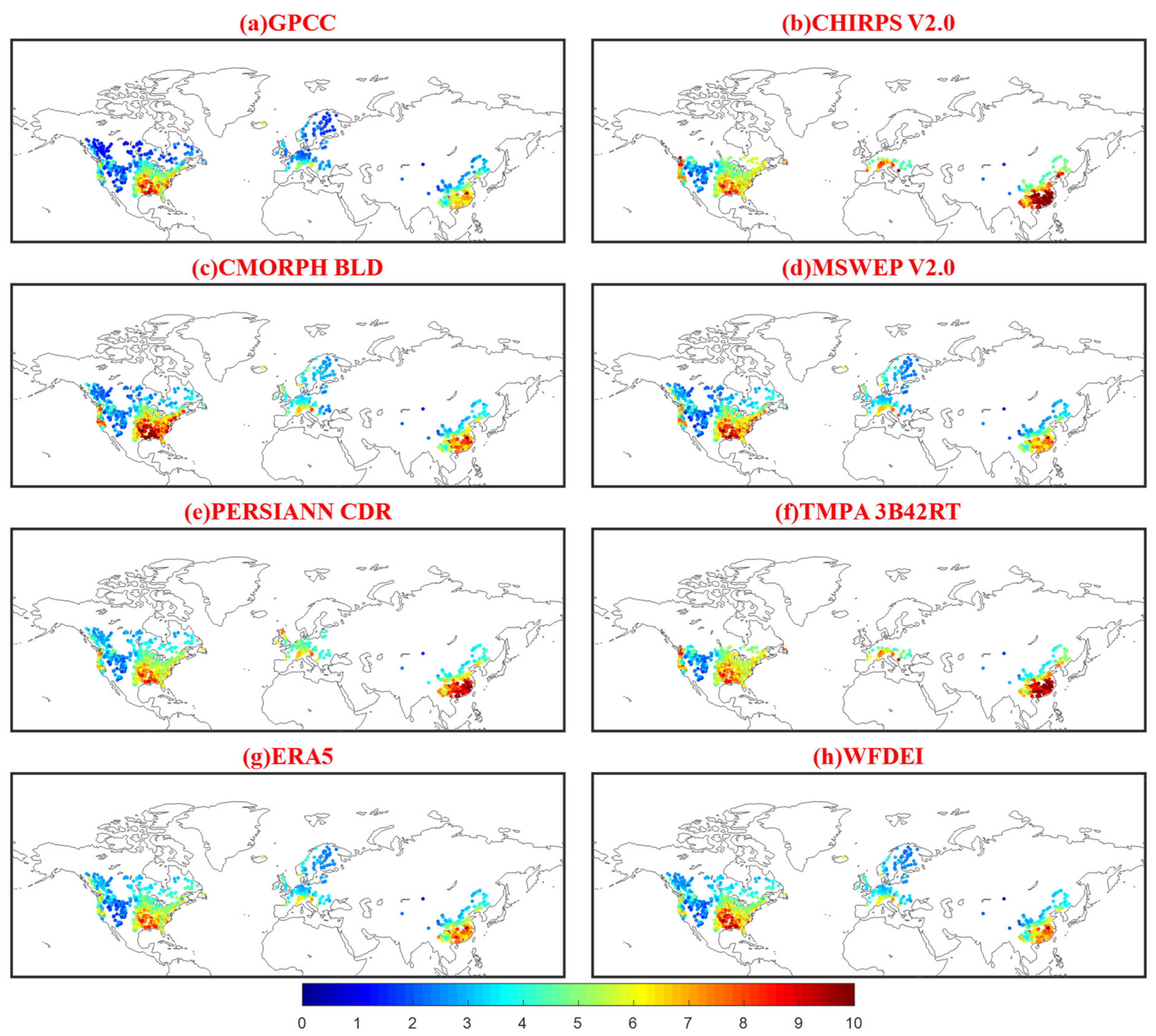
Figure 3 presents the spatial patterns of R3day between eight PPs and rain gauge observations (see the Appendix A for Spatial patterns of RB and RMSE). It shows that GPCC and MSWEP V2.0 exhibit R3day scores higher than 0.8 over most of these catchments. While PERSIANN CDR exhibits generally poor performances, which is consistent with the finding of previous evaluations [11,68] that IR-based datasets perform worse than PMW-based ones in precipitation estimation. The two reanalysis datasets, ERA5 and WFDEI, exhibit very similar performance. Regionally, PERSIANN CDR, CHIRPS V2.0, and TMPA 3B42RT perform relatively worse in Europe with median R3day scores of 0.49, 0.58 and 0.59. For China and North America, respectively, the worst performances for both are attained by PERSIANN CDR with median R3day scores of 0.64 and 0.69. All these PPs show relatively higher R3day scores over Western Europe, Eastern US and Southeastern China, where the density of observations is relatively high. Conversely, all exhibit worse performances over topographically complex regions such as the Balkan region, Southwestern China and the Andes. In terms of R3day, RB and RMSE, there generally exist larger discrepancies among the eight PPs over topographically complex mountainous regions, implying difficulties in estimating precipitation in these regions [11].
4.2. Evaluation of Hydrological Modeling
4.2.1. Benchmark Performance of Streamflow Simulation with Gauge-Observed Precipitation
In this Section, the XAJ model is calibrated by using rain gauge observations over 1382 catchments to test its performance and to provide the benchmark value for subsequent hydrological modeling with eight PPs. Figure 4 presents the spatial patterns and Cumulative Distribution Function (CDF) of NSE for both calibration and validation periods. The CDF of NSE shows that the median NSE scores are 0.79 and 0.66 for the calibration and validation periods, respectively. The spatial patterns of NSE show that the XAJ model driven by rain gauge observations can achieve good performances over most catchments, although there are relatively low NSE scores over the US Great Plains, which might be due to the spatially-temporally highly intermittent rainfall regime combined with a strongly nonlinear rainfall–runoff response, and over the Balkan region, which is presumably due to the low E-OBS rain-gauge density. In general, the results demonstrate satisfactory performance of the XAJ model based on the observations, which can be served as a benchmark for the hydrological performance evaluation of PPs.
4.2.2. Evaluation of Streamflow Simulations with Eight PPs
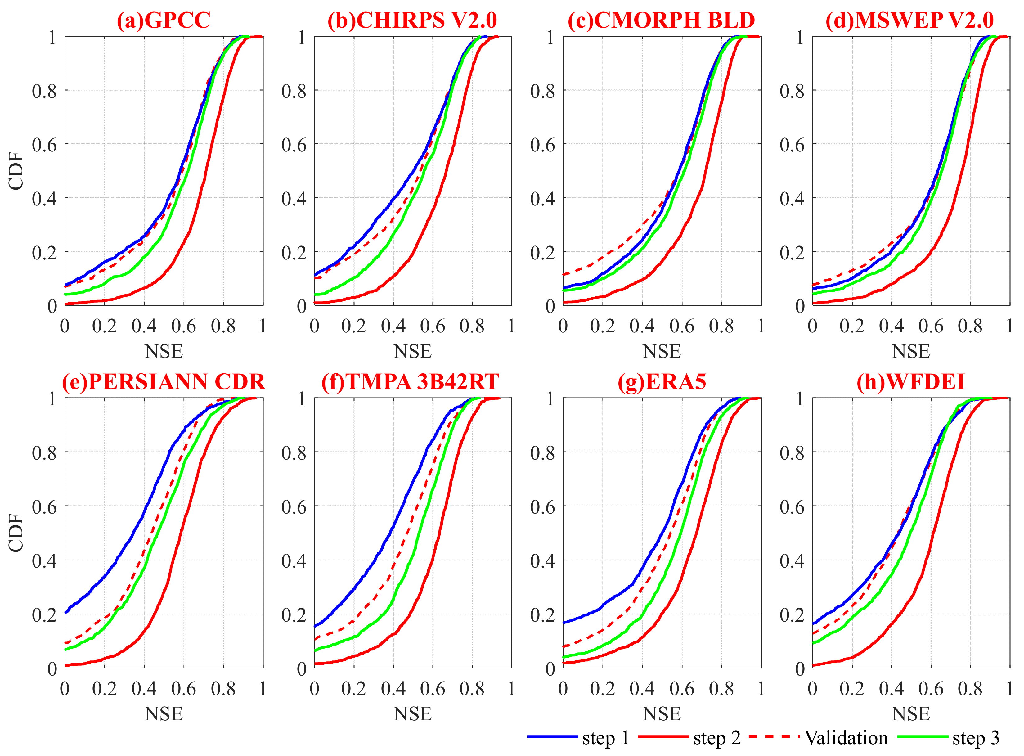
In this Section, the evaluations of streamflow simulations with eight PPs are based on three steps (see Section 3 for details). Table 2 presents the median NSE scores of eight PPs in reproducing the observed streamflow over 1382 catchments for all three steps. Figure 5 shows the CDF of NSE scores. It should be noted that CDF of steps 1~3 (solid line) is derived for the calibration period, and CDF of ‘validation’ (dashed line) refers to the performances for the validation period when applying PPs-specific calibration (in step 2).
Table 2 shows that the overall performance ranking of the PPs in step 1 from best to worst is MSWEP V2.0, CMORPH BLD, GPCC, CHIRPS V2.0, ERA5, WFDEI, TMPA 3B42RT and PERSIANN CDR. This indicates that the datasets incorporating daily gauge data (i.e., MSWEP V2.0, and CMORPH BLD) overall outperform those incorporating 5-day (i.e., CHIRPS V2.0) or monthly (i.e., TMPA 3B42RT, WFDEI, and PERSIANN CDR) gauge data. In comparison with GPCC, the superior performances of MSWEP V2.0 and CMORPH BLD also underscore the effectiveness of incorporating multiple satellite and reanalysis datasets.
In step 2, the hydrological modeling performances of the eight PPs are overall improved by PPs-specific calibration, with the highest NSE score for MSWEP V2.0 and the lowest NSE score for PERSIANN CDR, which is consistent with the (highest and lowest) performance ranking from step 1. Nevertheless, the absolute improvement is larger for the PPs with poor performances (i.e., TMPA 3B42RT, and PERSIANN CDR) than those with good performances (i.e., MSWEP V2.0, CMORPH BLD, and GPCC) in step 1. In addition, the bias correction in step 3 also improves the hydrological modeling performance for all PPs, with large improvement for those with large biases (i.e., TMPA 3B42RT, PERSIANN CDR and ERA5), which can be seen in Figure 2b. However, the effect of bias correction is negligible for the PPs with good performances in step 1 (i.e., MSWEP V2.0, CMORPH BLD, and GPCC). It can also be seen that the CDFs in steps 2 and 3 have consistently higher NSE scores than that in step 1, i.e., the mean median values of NSE are 0.50, 0.67, and 0.56 from steps 1,2 and 3, respectively. This demonstrates that the PPs used in this study can result in better performances of hydrological modeling after applying a PPs-specific calibration or bias correction method.
According to studies of Moriasi and Arnold [69] and Knoben and Freer [70], streamflow simulation can be considered to be satisfactory if NSE > 0.5. Based on that, the XAJ driven by gauge-observed precipitation can provide satisfy performances over 90% catchments in the calibration (Figure 4a) and 70% catchments in the validation period (Figure 4c). As for the hydrological modeling performances of PPs, in step 1, there are approximately 20% (PERSIANN CDR, blue line in Figure 5e) ~70% (MSWEP V2.0, blue line in Figure 5d) catchments above the corresponding threshold for NSE. There are more than 70% (PERSIANN CDR, red line in Figure 5e) ~90% (GPCC, red line in Figure 5a), and 40% (PERSIANN CDR, green line in Figure 5e) ~75% (MSWEP V2.0, green line in Figure 4d) catchments above the corresponding threshold in step 2 and step 3, respectively. Figure 5 also shows the hydrological modeling performances during the validation period when PPs-specific calibration is used. There are about 40% (PERSIANN CDR, dash line in Figure 5e) ~70% (MSWEP V2.0, dash line in Figure 5d) catchments above the corresponding threshold. The results above indicate that the PPs have good potential for hydrological modeling, which is consistent with recent findings [71,72]. What is more, the best performance of MSWEP V2.0 among the PPs shows that, to a certain extent, it can be used as an alternative forcing to hydrological modeling of XAJ where a lack of gauge precipitation observations exists.
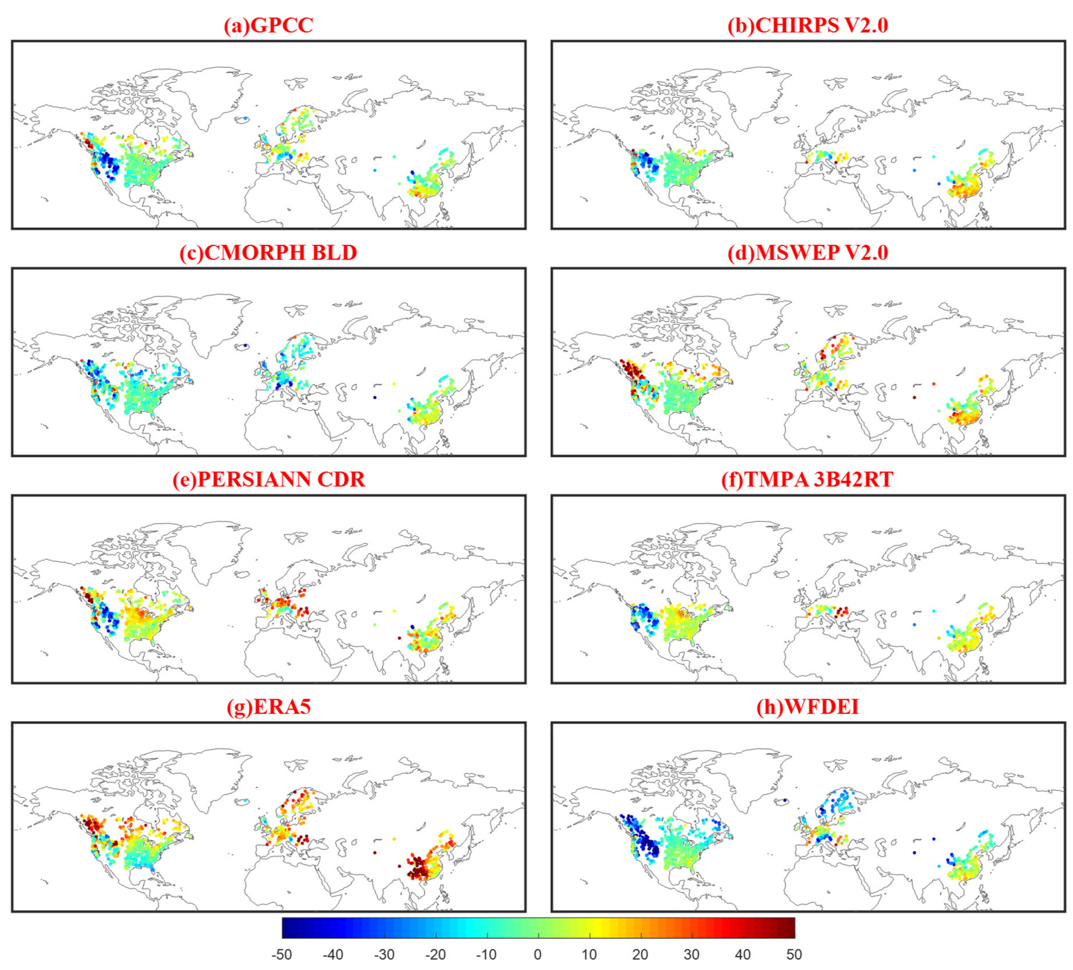
Figure 6 presents the spatial patterns of NSE for the eight PPs obtained by running XAJ with ‘RP’ (step 1). MSWEP V2.0, GPCC and CMORPH BLD generally exhibit good performances in Eastern US, Southeastern China, Northern and Western Europe, even with MSWEP V2.0 and GPCC outperforming the gauge-observed precipitation in Europe. All the PPs provide low NSE scores over the US Great Plains, especially for GPCC, PERSIANN CDR, TMPA 3B42RT, and WFDEI (<0.2), which is consistent with previous findings using different hydrological models and precipitation datasets [26,71]. Low NSE scores are also found for CHIRPS V2.0, TMPA 3B42RT and ERA5 in China, and for PERSIANN CDR in both China and Europe. There are some PPs performing better than others regionally, but there is no one outperforming everywhere. For instance, MSWEP V2.0 generally shows better performances in most places, but it tends to perform worse than PERSIANN CDR in the northern part of Rocky Mountains. For each PPs, the NSE scores are relatively higher in temperate regions than in arid or topographically complex mountainous regions, due to the sparse rain-gauge networks and the highly non-linear rainfall-runoff response.
Figure 7 shows the PPs with the highest improvement in NSE by applying PPs-specific calibration (step 2) and bias correction (step 3) relative to step 1. The spatial pattern of the PPs with the largest improvement in NSE by using PPs-specific calibration (Figure 7a) is similar with that by using bias correction (Figure 7b). There are higher improvements for ERA5, WFDEI, PERSIANNCDR and TMPA 3B42RT over Southeastern US, Northern Europe, Western Europe and most watersheds in China, respectively. This is in accordance with the observation that these datasets show worse initial performances over these regions.
In addition, RB is used to further explore whether the PPs can be used to estimate the annual streamflow and the results are shown in Figure 8. The RB derived from gauge-observed precipitation (Obs) is also displayed, which provides a satisfied estimation for the annual streamflow with a slight underestimation. The MSWEP V2.0 with the highest NSE values (median: 0.63) has the lowest error in annual streamflow (median: −1.63). The good performance of MSWEP V2.0 in terms of both NSE and RB indicate that we can use MSWEP V2.0 as an alternative precipitation data source for hydrologic modeling when facing a lack of gauge precipitation observations. For the eight PPs, the median values of absolute RB in step 2 (mean: 4.57) and step 3 (mean: 6.94) are lower than that in step 1 (mean: 9.32). This demonstrates that specific calibration and bias correction can effectively improve the abilities of the PPs in the annual streamflow estimates.
5. Conclusions
This study comprehensively evaluated eight widely used PPs including GPCC, CHIRPS V2.0, CMORPH BLD, PERSIANN CDR, TMPA 3B42RT, MSWEP V2.0, ERA5 and WFDEI in hydrological modeling over 1382 catchments in China, Europe and North America during the 1998-2015 period at a daily temporal scale. The PPs-specific calibration and bias correction method has also been included in the hydrological evaluation and discussion. The following conclusions can be drawn:
- (1)
- Compared with the gauge-observed precipitation, GPCC provides the best performance overall, followed by MSWEP V2.0, which is merged based on multiple satellite and reanalysis datasets.
- (2)
- Among all the PPs, MSWEP V2.0 and CMORPH BLD, which incorporate daily gauge data provide superior hydrological performance, followed by those incorporating 5-day (CHIRPS V2.0) and monthly (TMPA 3B42RT, WFDEI, and PERSIANN CDR) gauge data. MSWEP V2.0 and CMORPH BLD perform better than GPCC, underscoring the effectiveness of merging multiple satellite and reanalysis datasets.
- (3)
- Regionally, all PPs exhibit better performances in temperate regions than in arid or topographically complex mountainous regions, due to the sparse rain-gauge networks and the highly non-linear rainfall-runoff response. Uncertainty exists in the regional performances of all the PPs.
- (4)
- PPs-specific calibration and bias correction both can improve the streamflow simulations for all eight PPs in terms of the Nash and Sutcliffe efficiency and the absolute bias. The improvements in hydrological modeling performances are larger for the PPs with poor performances.
Overall, this study investigates the reliabilities of PPs in hydrological applications, as well as the approaches to improve their hydrological modeling performances. There are still some limitations. For example, the catchments are located in China, Europe and North America with dense rain-gauge networks and these conclusions may not generalize to regions with sparse rain-gauge networks. In addition, some different results may be derived when using another hydrological model, calibration objective function or temperature or evaporation forcing. These problems therefore should be investigated in future studies to generalize the conclusions in this study.
Author Contributions
Conceptualization, L.L.; Data curation, Y.X.; Formal analysis, Y.X.; Funding acquisition, J.C. and T.P.; Investigation, Y.X.; Methodology, J.C. and L.L; Resources, J.C.; Validation, T.P. and Z.Y.; Writing—original draft, Y.X.; Writing—review & editing, J.C. and L.L. All authors have read and agreed to the published version of the manuscript.
Funding
This work was partially supported by the National Key Research and Development Program of China (No. 2017YFA0603704), the National Natural Science Foundation of China (Grant No. 52079093), the Hubei Provincial Natural Science Foundation of China (Grant No. 2020CFA100) and the National Key Research and Development Program of China (2018YFC1507204).
Acknowledgments
The authors would like to acknowledge all of the organizations for providing the global precipitation datasets, namely, the Global Precipitation Climatology Centre (GPCC), Climate Hazards Group (CHIRPS V2.0), NOAA Climate Prediction Center (CMORPH BLD), NOAA National Climatic Data Center (PERSIANN CDR), Goddard Earth Sciences Data and Information Services Center (TMPA 3B42RT), Hylke Beck from Princeton University, the developer of MSWEP V2.0, European Centre For Medium Range Weather Forecasts (ERA5) and Graham P. Weedon from Hydrometeorological Research, Wallingford, UK, the developer of WFDEI. The authors also thank the China Meteorological Data Sharing System, the Europe Climate Assessment & Dataset project, the Canadian model parameter experiment (CANOPEX) database and the Santa Clara database for providing gauge-observed precipitation and temperature. In addition, the authors thank the Global Runoff Data Center, the CANOPEX and the United States Geological Survey (USGS) database for providing observed streamflow, as well as Brecht Martens from Ghent University, the developer of GLEAM.
Conflicts of Interest
The authors declare no conflict of interest.
Appendix A
Figure A1.
Spatial patterns of RB for the eight PPs using gauge-observed precipitation from 1382 catchments as a reference. Each data point represents a catchment centroid.
Figure A1.
Spatial patterns of RB for the eight PPs using gauge-observed precipitation from 1382 catchments as a reference. Each data point represents a catchment centroid.

Figure A2.
Spatial patterns of RMSE for the eight PPs using gauge-observed precipitation from 1382 catchments as a reference. Each data point represents a catchment centroid.
Figure A2.
Spatial patterns of RMSE for the eight PPs using gauge-observed precipitation from 1382 catchments as a reference. Each data point represents a catchment centroid.
References
- Trenberth, K.E.; Dai, A.; Rasmussen, R.M.; Parsons, D.B. The Changing Character of Precipitation. Bull. Am. Meteorol. Soc. 2003, 84, 1205–1218. [Google Scholar] [CrossRef]
- Eltahir, E.A.B.; Bras, R.L. Precipitation recycling. Rev. Geophys. 1996, 34, 367–378. [Google Scholar] [CrossRef]
- Hou, A.Y.; Kakar, R.K.; Neeck, S.; Azarbarzin, A.A.; Kummerow, C.D.; Kojima, M.; Oki, R.; Nakamura, K.; Iguchi, T. The global precipitation measurement mission. Bull. Am. Meteorol. Soc. 2014, 95, 701–722. [Google Scholar] [CrossRef]
- Kidd, C.; Huffman, G. Global precipitation measurement. Meteorol. Appl. 2011, 18, 334–353. [Google Scholar] [CrossRef]
- Larson, L.W.; Peck, E.L. Accuracy of precipitation measurements for hydrologic modeling. Water Resour. Res. 1974, 10, 857–863. [Google Scholar] [CrossRef]
- Maggioni, V.; Meyers, P.C.; Robinson, M.D. A Review of Merged High-Resolution Satellite Precipitation Product Accuracy during the Tropical Rainfall Measuring Mission (TRMM) Era. J. Hydrometeorol. 2016, 17, 1101–1117. [Google Scholar] [CrossRef]
- Sun, Q.; Miao, C.; Duan, Q.; Ashouri, H.; Sorooshian, S.; Hsu, K.L. A review of global precipitation data sets: Data sources, estimation, and intercomparisons. Rev. Geophys. 2018, 56, 79–107. [Google Scholar] [CrossRef] [Green Version]
- Alijanian, M.; Rakhshandehroo, G.; Mishra, A.K.; Dehghani, M. Evaluation of satellite rainfall climatology using CMORPH, PERSIANN-CDR, PERSIANN, TRMM, MSWEP over Iran. Int. J. Clim. 2017, 37, 4896–4914. [Google Scholar] [CrossRef]
- Buarque, D.C.; Paiva, R.; Clarke, R.T.; Mendes, C.A.B. A comparison of Amazon rainfall characteristics derived from TRMM, CMORPH and the Brazilian national rain gauge network. J. Geophys. Res. Space Phys. 2011, 116. [Google Scholar] [CrossRef]
- Bumke, K.; König-Langlo, G.; Kinzel, J.; Schröder, M. HOAPS and ERA-Interim precipitation over the sea: Validation against shipboard in situ measurements. Atmos. Meas. Tech. 2016, 9, 2409–2423. [Google Scholar] [CrossRef] [Green Version]
- Hirpa, F.A.; Gebremichael, M.; Hopson, T. Evaluation of High-Resolution Satellite Precipitation Products over Very Complex Terrain in Ethiopia. J. Appl. Meteorol. Clim. 2010, 49, 1044–1051. [Google Scholar] [CrossRef]
- AghaKouchak, A.; Behrangi, A.; Sorooshian, S.; Hsu, K.; Amitai, E. Evaluation of satellite-retrieved extreme precipitation rates across the central United States. J. Geophys. Res. Space Phys. 2011, 116. [Google Scholar] [CrossRef]
- Islam, T.; Rico-Ramirez, M.A.; Han, D.; Srivastava, P.K.; Ishak, A.M. Performance evaluation of the TRMM precipitation estimation using ground-based radars from the GPM validation network. J. Atmos. Sol. Terr. Phys. 2012, 77, 194–208. [Google Scholar] [CrossRef]
- Bosilovich, M.G.; Chen, J.; Robertson, F.R.; Adler, R.F. Evaluation of Global Precipitation in Reanalyses. J. Appl. Meteorol. Clim. 2008, 47, 2279–2299. [Google Scholar] [CrossRef]
- Kalnay, E.; Kanamitsu, M.; Kistler, R.; Collins, W.; Deaven, D.; Gandin, L.; Iredell, M.; Saha, S.; White, G.; Woollen, J.; et al. The NCEP/NCAR 40-year reanalysis project. Bull. Am. Meteorol. Soc. 1996, 77, 437–472. [Google Scholar] [CrossRef] [Green Version]
- Uppala, S.M.; Kållberg, P.W.; Simmons, A.J.; Andrae, U.; Bechtold VD, C.; Fiorino, M.; Gibson, J.K.; Haseler, J.; Hernandez, A.; Kelly, G.A.; et al. The ERA-40 re-analysis. Q. J. R. Meteorol. Soc. A J. Atmos. Sci. Appl. Meteorol. Phys. Oceanogr. 2005, 131, 2961–3012. [Google Scholar] [CrossRef]
- Onogi, K.; Tsutsui, J.; Koide, H.; Sakamoto, M.; Kobayashi, S.; Hatsushika, H.; Matsumoto, T.; Yamazaki, N.; Kamahori, H.; Takahashi, K.; et al. The JRA-25 Reanalysis. J. Meteorol. Soc. Jpn. 2007, 85, 369–432. [Google Scholar] [CrossRef] [Green Version]
- Beck, H.E.; Pan, M.; Roy, T.; Weedon, G.P.; Pappenberger, F.; Van Dijk, A.I.; Huffman, G.J.; Adler, R.F.; Wood, E.F. Daily evaluation of 26 precipitation datasets using Stage-IV gauge-radar data for the CONUS. Hydrol. Earth Syst. Sci. 2019, 23, 207–224. [Google Scholar] [CrossRef] [Green Version]
- Beck, H.E.; Van Dijk, A.I.J.M.; Levizzani, V.; Schellekens, J.; Miralles, D.; Martens, B.; De Roo, A. MSWEP: 3-hourly 0.25° global gridded precipitation (1979–2015) by merging gauge, satellite, and reanalysis data. Hydrol. Earth Syst. Sci. 2017, 21, 589–615. [Google Scholar] [CrossRef] [Green Version]
- Hersbach, H.; Bell, B.; Berrisford, P.; Hirahara, S.; Horanyi, A.; Muñoz-Sabater, J.; Nicolas, J.; Peubey, C.; Radu, R.; Schepers, D.; et al. The ERA5 global reanalysis. Q. J. R. Meteorol. Soc. 2020, 146, 1999–2049. [Google Scholar] [CrossRef]
- Behrangi, A.; Khakbaz, B.; Jaw, T.C.; AghaKouchak, A.; Hsu, K.; Sorooshian, S. Hydrologic evaluation of satellite precipitation products over a mid-size basin. J. Hydrol. 2011, 397, 225–237. [Google Scholar] [CrossRef] [Green Version]
- Bitew, M.M.; Gebremichael, M.; Ghebremichael, L.T.; Bayissa, Y.A. Evaluation of high-resolution satellite rainfall products through streamflow simulation in a hydrological modeling of a small mountainous watershed in Ethiopia. J. Hydrometeorol. 2012, 13, 338–350. [Google Scholar] [CrossRef]
- Collischonn, B.; Collischonn, W.; Tucci, C.E.M. Daily hydrological modeling in the Amazon basin using TRMM rainfall estimates. J. Hydrol. 2008, 360, 207–216. [Google Scholar] [CrossRef]
- Li, X.; Chen, Y.; Deng, X.; Zhang, Y.; Chen, L. Evaluation and Hydrological Utility of the GPM IMERG Precipitation Products over the Xinfengjiang River Reservoir Basin, China. Remote. Sens. 2021, 13, 866. [Google Scholar] [CrossRef]
- Huffman, G.J.; Bolvin, D.T.; Nelkin, E.J. Integrated Multi-satellitE Retrievals for GPM (IMERG) technical documentation. Nasa/Gsfc Code 2015, 612, 2019. [Google Scholar]
- Beck, H.E.; Vergopolan, N.; Pan, M.; Levizzani, V.; Van Dijk, A.I.J.M.; Weedon, G.P.; Brocca, L.; Pappenberger, F.; Huffman, G.J.; Wood, E.F. Global-scale evaluation of 22 precipitation datasets using gauge observations and hydrological modeling. Hydrol. Earth Syst. Sci. 2017, 21, 6201–6217. [Google Scholar] [CrossRef] [Green Version]
- Camici, S.; Ciabatta, L.; Massari, C.; Brocca, L. How reliable are satellite precipitation estimates for driving hydrological models: A verification study over the Mediterranean area. J. Hydrol. 2018, 563, 950–961. [Google Scholar] [CrossRef]
- Yilmaz, K.K.; Hogue, T.S.; Hsu, K.-L.; Sorooshian, S.; Gupta, H.; Wagener, T. Intercomparison of Rain Gauge, Radar, and Satellite-Based Precipitation Estimates with Emphasis on Hydrologic Forecasting. J. Hydrometeorol. 2005, 6, 497–517. [Google Scholar] [CrossRef]
- Mei, Y.; Anagnostou, E.N.; Nikolopoulos, E.; Borga, M. Error Analysis of Satellite Precipitation Products in Mountainous Basins. J. Hydrometeorol. 2014, 15, 1778–1793. [Google Scholar] [CrossRef]
- Qi, W.; Zhang, C.; Fu, G.; Sweetapple, C.; Zhou, H. Evaluation of global fine-resolution precipitation products and their uncertainty quantification in ensemble discharge simulations. Hydrol. Earth Syst. Sci. 2016, 20, 903–920. [Google Scholar] [CrossRef] [Green Version]
- Hughes, D.A. Comparison of satellite rainfall data with observations from gauging station networks. J. Hydrol. 2006, 327, 399–410. [Google Scholar] [CrossRef]
- Ciabatta, L.; Brocca, L.; Massari, C.; Moramarco, T.; Gabellani, S.; Puca, S.; Wagner, W. Rainfall-runoff modelling by using SM2RAIN-derived and state-of-the-art satellite rainfall products over Italy. Int. J. Appl. Earth Obs. Geoinf. 2016, 48, 163–173. [Google Scholar] [CrossRef]
- Huffman, G.J.; Bolvin, D.T.; Nelkin, E.J.; Wolff, D.B.; Adler, R.F.; Gu, G.; Hong, Y.; Bowman, K.P.; Stocker, E.F. The TRMM Multisatellite Precipitation Analysis (TMPA): Quasi-Global, Multiyear, Combined-Sensor Precipitation Estimates at Fine Scales. J. Hydrometeorol. 2007, 8, 38–55. [Google Scholar] [CrossRef]
- Chen, F.; Gao, Y. Evaluation of precipitation trends from high-resolution satellite precipitation products over Mainland China. Clim. Dyn. 2018, 51, 3311–3331. [Google Scholar] [CrossRef]
- Jiang, S.H.; Ren, L.L.; Yong, B.; Yang, X.L.; Shi, L. Evaluation of high-resolution satellite precipitation products with surface rain gauge observations from Laohahe Basin in northern China. Water Sci. Eng. 2010, 3, 405–417. [Google Scholar]
- Ashouri, H.; Sorooshian, S.; Hsu, K.-L.; Bosilovich, M.G.; Lee, J.; Wehner, M.F.; Collow, A. Evaluation of NASA’s MERRA Precipitation Product in Reproducing the Observed Trend and Distribution of Extreme Precipitation Events in the United States. J. Hydrometeorol. 2016, 17, 693–711. [Google Scholar] [CrossRef] [Green Version]
- Kishore, P.; Jyothi, S.; Basha, G.; Rao, S.V.B.; Rajeevan, M.; Velicogna, I.; Sutterley, T. Precipitation climatology over India: Validation with observations and reanalysis datasets and spatial trends. Clim. Dyn. 2015, 46, 541–556. [Google Scholar] [CrossRef] [Green Version]
- Gao, Y.; Liu, M. Evaluation of high-resolution satellite precipitation products using rain gauge observations over the Tibetan Plateau. Hydrol. Earth Syst. Sci. 2013, 17, 837–849. [Google Scholar] [CrossRef] [Green Version]
- Liu, J.; Zhu, A.-X.; Duan, Z. Evaluation of TRMM 3b42 precipitation product using rain gauge data in Meichuan Watershed, Poyang Lake Basin, China. J. Resour. Ecol. 2012, 3, 359–366. [Google Scholar]
- Schneider, U.; Fuchs, T.; Meyer-Christoffer, A.; Rudolf, B. Global precipitation analysis products of the GPCC. Glob. Precip. Climatol. Cent. DwdInternet Publ. 2008, 112, 1–14. [Google Scholar]
- Peterson, P. The Climate Hazards Group InfraRed Precipitation with Stations (CHIRPS) v2.0 Dataset: 35 year Quasi-Global Precipitation Estimates for Drought Monitoring. Sci. Data 2014, 2, 1–21. [Google Scholar]
- Joyce, R.J.; Janowiak, J.E.; Arkin, P.A.; Xie, P. CMORPH: A method that produces global precipitation estimates from passive microwave and infrared data at high spatial and temporal resolution. J. Hydrometeorol. 2004, 5, 487–503. [Google Scholar] [CrossRef]
- Ashouri, H.; Hsu, K.-L.; Sorooshian, S.; Braithwaite, D.K.; Knapp, K.; Cecil, L.D.; Nelson, B.R.; Prat, O. PERSIANN-CDR: Daily Precipitation Climate Data Record from Multisatellite Observations for Hydrological and Climate Studies. Bull. Am. Meteorol. Soc. 2015, 96, 69–83. [Google Scholar] [CrossRef] [Green Version]
- Weedon, G.P.; Balsamo, G.; Bellouin, N.; Gomes, S.; Best, M.; Viterbo, P. The WFDEI meteorological forcing data set: WATCH Forcing Data methodology applied to ERA-Interim reanalysis data. Water Resour. Res. 2014, 50, 7505–7514. [Google Scholar] [CrossRef] [Green Version]
- Haylock, M.R.; Hofstra, N.; Tank, A.K.; Klok, E.J.; Jones, P.; New, M. A European daily high-resolution gridded data set of surface temperature and precipitation for 1950–2006. J. Geophys. Res. Space Phys. 2008, 113, 20. [Google Scholar] [CrossRef] [Green Version]
- Arsenault, R.; Bazile, R.; Dallaire, C.O.; Brissette, F. CANOPEX: A Canadian hydrometeorological watershed database. Hydrol. Process. 2016, 30, 2734–2736. [Google Scholar] [CrossRef]
- Maurer, E.P.; Wood, A.W.; Adam, J.C.; Lettenmaier, D.P.; Nijssen, B. A long-term hydrologically based dataset of land surface fluxes and states for the conterminous United States. J. Clim. 2002, 15, 3237–3251. [Google Scholar] [CrossRef] [Green Version]
- Martens, B.; Gonzalez Miralles, D.; Lievens, H.; Van Der Schalie, R.; De Jeu, R.A.M.; Fernández-Prieto, D.; Beck, H.E.; Dorigo, W.A.; Verhoest, N.E.C. GLEAM v3: Satellite-based land evaporation and root-zone soil moisture. Geosci. Model Dev. 2017, 10, 1903–1925. [Google Scholar] [CrossRef] [Green Version]
- Falcone, J.A.; Carlisle, D.M.; Wolock, D.M.; Meador, M.R. GAGES: A stream gage database for evaluating natural and altered flow conditions in the conterminous United States. Ecology 2010, 91, 621. [Google Scholar] [CrossRef]
- Mizukami, N.; Smith, M.B. Analysis of inconsistencies in multi-year gridded quantitative precipitation estimate over complex terrain and its impact on hydrologic modeling. J. Hydrol. 2012, 428–429, 129–141. [Google Scholar] [CrossRef] [Green Version]
- Zhao, Y.; Zhu, J. Assessing Quality of Grid Daily Precipitation Datasets in China in Recent 50 Years. Plateau Meteorol. 2015, 34, 50–58. [Google Scholar]
- Miralles, D.G.; Holmes, T.R.H.; De Jeu, R.A.M.; Gash, J.H.; Meesters, A.G.C.A.; Dolman, A.J. Global land-surface evaporation estimated from satellite-based observations. Hydrol. Earth Syst. Sci. 2011, 15, 453–469. [Google Scholar] [CrossRef] [Green Version]
- Hagemann, S.; Dümenil, L. A parametrization of the lateral waterflow for the global scale. Clim. Dyn. 1997, 14, 17–31. [Google Scholar] [CrossRef]
- Zhao, R.; Liu, X. The Xinanjiang Model, Computer Models of Watershed Hydrology; Singh, V.P., Ed.; Water Resources Publications: California City, CA, USA, 1995; pp. 215–232. [Google Scholar]
- Li, L.; Ngongondo, C.S.; Xu, C.-Y.; Gong, L. Comparison of the global TRMM and WFD precipitation datasets in driving a large-scale hydrological model in southern Africa. Hydrol. Res. 2012, 44, 770–788. [Google Scholar] [CrossRef]
- Zeng, Q.; Chen, H.; Xu, C.-Y.; Jie, M.-X.; Hou, Y.-K. Feasibility and uncertainty of using conceptual rainfall-runoff models in design flood estimation. Hydrol. Res. 2015, 47, 701–717. [Google Scholar] [CrossRef] [Green Version]
- Chen, J.; Li, Z.; Li, L.; Wang, J.; Qi, W.; Xu, C.-Y.; Kim, J.-S. Evaluation of Multi-Satellite Precipitation Datasets and Their Error Propagation in Hydrological Modeling in a Monsoon-Prone Region. Remote. Sens. 2020, 12, 3550. [Google Scholar] [CrossRef]
- Valéry, A.; Andréassian, V.; Perrin, C. ’As simple as possible but not simpler’: What is useful in a temperature-based snow-accounting routine? Part 1—Comparison of six snow accounting routines on 380 catchments. J. Hydrol. 2014, 517, 1166–1175. [Google Scholar] [CrossRef]
- Duan, Q.; Gupta, V.K.; Sorooshian, S. Shuffled complex evolution approach for effective and efficient global minimization. J. Optim. Theory Appl. 1993, 76, 501–521. [Google Scholar] [CrossRef]
- Nash, J.E.; Sutcliffe, J.V. River flow forecasting through conceptual models part I—A discussion of principles. J. Hydrol. 1970, 10, 282–290. [Google Scholar] [CrossRef]
- Chen, J.; Brissette, F.P.; Chaumont, D.; Braun, M. Performance and uncertainty evaluation of empirical downscaling methods in quantifying the climate change impacts on hydrology over two North American river basins. J. Hydrol. 2013, 479, 200–214. [Google Scholar] [CrossRef]
- Schmidli, J.; Frei, C.; Vidale, P.L. Downscaling from GCM precipitation: A benchmark for dynamical and statistical downscaling methods. Int. J. Clim. 2006, 26, 679–689. [Google Scholar] [CrossRef]
- Mpelasoka, F.S.; Chiew, F.H.S. Influence of Rainfall Scenario Construction Methods on Runoff Projections. J. Hydrometeorol. 2009, 10, 1168–1183. [Google Scholar] [CrossRef]
- Schneider, U.; Becker, A.; Finger, P.; Meyer-Christoffer, A.; Ziese, M.; Rudolf, B. GPCC’s new land surface precipitation climatology based on quality-controlled in situ data and its role in quantifying the global water cycle. Theor. Appl. Climatol. 2014, 115, 15–40. [Google Scholar] [CrossRef] [Green Version]
- Jiang, Q.; Li, W.; Fan, Z.; He, X.; Sun, W.; Chen, S.; Wen, J.; Gao, J.; Wang, J. Evaluation of the ERA5 reanalysis precipitation dataset over Chinese Mainland. J. Hydrol. 2021, 595, 125660. [Google Scholar] [CrossRef]
- Funk, C.; Peterson, P.; Landsfeld, M.; Pedreros, D.; Verdin, J.; Shukla, S.; Husak, G.; Rowland, J.; Harrison, L.; Hoell, A.; et al. The climate hazards infrared precipitation with stations—a new environmental record for monitoring extremes. Sci. Data 2015, 2, 1–21. [Google Scholar] [CrossRef] [Green Version]
- Fick, S.E.; Hijmans, R.J. WorldClim 2: New 1-km spatial resolution climate surfaces for global land areas. Int. J. Clim. 2017, 37, 4302–4315. [Google Scholar] [CrossRef]
- Cattani, E.; Merino, A.; Levizzani, V. Evaluation of Monthly Satellite-Derived Precipitation Products over East Africa. J. Hydrometeorol. 2016, 17, 2555–2573. [Google Scholar] [CrossRef]
- Moriasi, D.N.; Arnold, J.G.; Van Liew, M.W.; Bingner, R.L.; Harmel, R.D.; Veith, T.L. Model Evaluation Guidelines for Systematic Quantification of Accuracy in Watershed Simulations. Trans. Asabe 2007, 50, 885–900. [Google Scholar] [CrossRef]
- Knoben, W.J.; Freer, J.E.; Woods, R.A. Inherent benchmark or not? Comparing Nash–Sutcliffe and Kling–Gupta efficiency scores. Hydrol. Earth Syst. Sci. 2019, 23, 4323–4331. [Google Scholar] [CrossRef] [Green Version]
- Essou, G.R.; Arsenault, R.; Brissette, F.P. Comparison of climate datasets for lumped hydrological modeling over the continental United States. J. Hydrol. 2016, 537, 334–345. [Google Scholar] [CrossRef]
- Raimonet, M.; Oudin, L.; Thieu, V.; Silvestre, M.; Vautard, R.; Rabouille, C.; Le Moigne, P. Evaluation of Gridded Meteorological Datasets for Hydrological Modeling. J. Hydrometeorol. 2017, 18, 3027–3041. [Google Scholar] [CrossRef]
Figure 1.
Flowchart of the XAJ model.

Figure 2.
Boxplots of (a) R calculated for 3-day means (R3day), (b) RB and (c) RMSE for the eight PPs using gauge-observed precipitation from 1382 catchments as a reference. The circles represent the median value, and the left and right edges of the box represent the 25th and 75th percentile values, respectively, while the “whiskers” represent the extreme values.
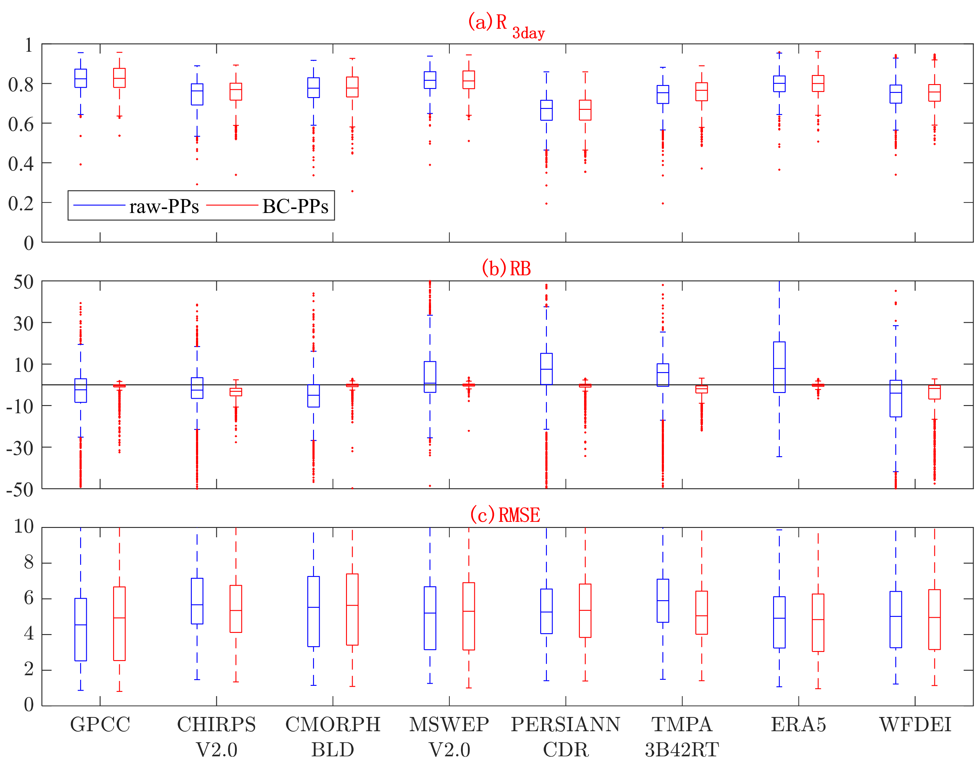
Figure 3.
Spatial patterns of the R calculated for 3-day means (R3day) for the eight PPs ((a) GPCC, (b) CHIRPS V2.0, (c) CMORPH BLD, (d) MSWEP V2.0, (e) PERSIANN CDR, (f) TMPA 3B42RT, (g) ERA5, (h) WFDEI) using gauge-observed precipitation from 1382 catchments as a reference. Each data point represents a catchment centroid.

Figure 4.
Spatial pattern and Cumulative Distribution Function (CDF) of NSE obtained by running XAJ with gauge-observed precipitation over 1382 catchments. (a,b) are for the calibration period, (c,d) are for the validation period.
Figure 4.
Spatial pattern and Cumulative Distribution Function (CDF) of NSE obtained by running XAJ with gauge-observed precipitation over 1382 catchments. (a,b) are for the calibration period, (c,d) are for the validation period.
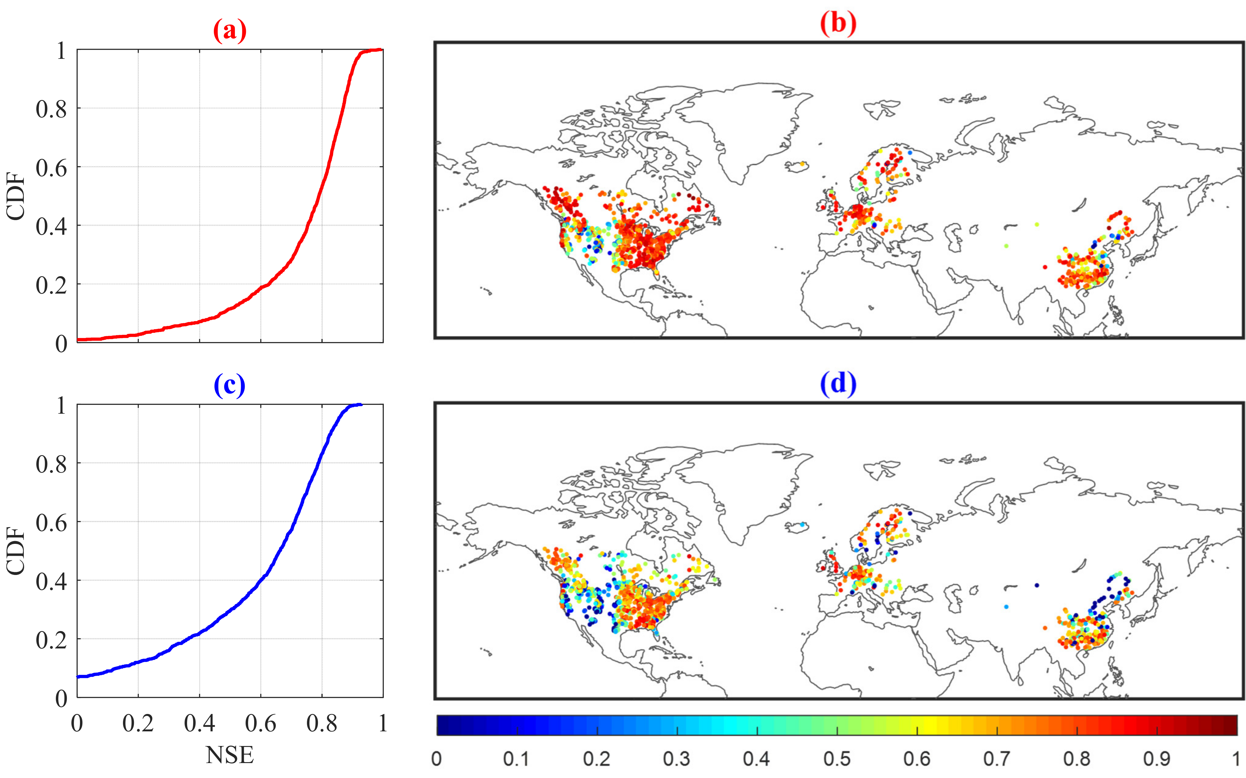
Figure 5.
Cumulative Distribution Function (CDF) of NSE obtained by running XAJ with the eight PPs ((a) GPCC, (b) CHIRPS V2.0, (c) CMORPH BLD, (d) MSWEP V2.0, (e) PERSIANN CDR, (f) TMPA 3B42RT, (g) ERA5, (h) WFDEI) over 1382 catchments based on 3 steps of hydrological modeling. The dash line refers to the validation when PPs-specific calibration is used.

Figure 6.
Spatial patterns of NSE for the eight PPs ((a) GPCC, (b) CHIRPS V2.0, (c) CMORPH BLD, (d) MSWEP V2.0, (e) PERSIANN CDR, (f) TMPA 3B42RT, (g) ERA5, (h) WFDEI) obtained by running XAJ with ‘RP’ over 1382 catchments (step 1).
Figure 6.
Spatial patterns of NSE for the eight PPs ((a) GPCC, (b) CHIRPS V2.0, (c) CMORPH BLD, (d) MSWEP V2.0, (e) PERSIANN CDR, (f) TMPA 3B42RT, (g) ERA5, (h) WFDEI) obtained by running XAJ with ‘RP’ over 1382 catchments (step 1).
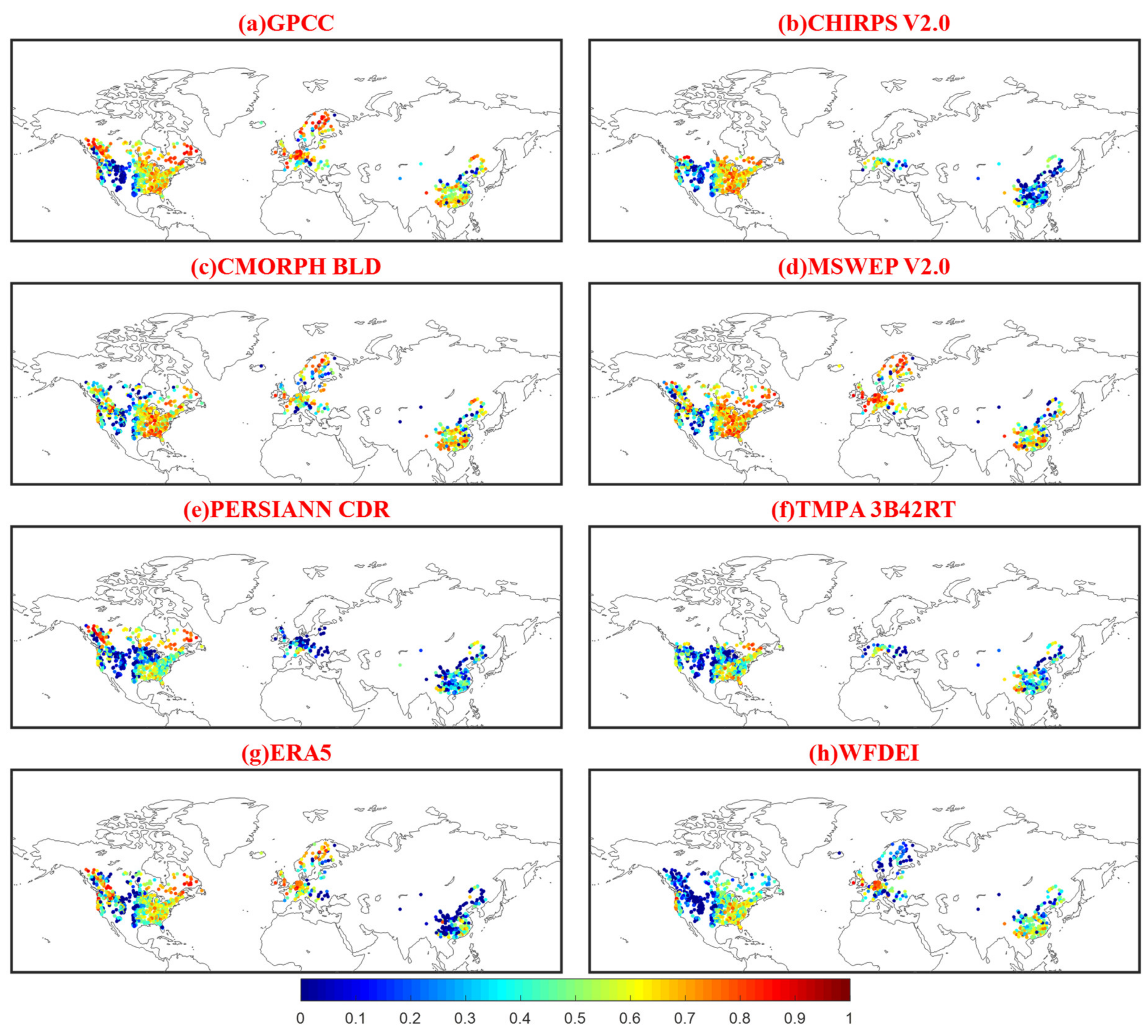
Figure 7.
For each catchment, the PPs with the highest improvement by applying (a) PPs-specific calibration (step 2) and (b) bias correction (step 3), compared with the NSE obtained by running XAJ with ‘RP’ (step 1).
Figure 7.
For each catchment, the PPs with the highest improvement by applying (a) PPs-specific calibration (step 2) and (b) bias correction (step 3), compared with the NSE obtained by running XAJ with ‘RP’ (step 1).

Figure 8.
Boxplots of RB for annual streamflow volume simulated by gauge-observed precipitation (Obs) and the eight PPs, with the observed streamflow over 1382 catchments as a reference. Boxplot representation is the same as Figure 1.
Figure 8.
Boxplots of RB for annual streamflow volume simulated by gauge-observed precipitation (Obs) and the eight PPs, with the observed streamflow over 1382 catchments as a reference. Boxplot representation is the same as Figure 1.


Table 1.
Overview of the datasets used in this study.
| Type | Name (Details) | Category | Temporal/Spatial Resolution | Temporal Coverage | Reference or Link |
|---|---|---|---|---|---|
| Global Precipitation Datasets | GPCC (Global Precipitation Climatology Centre) | G | Daily/global 0.5° | 1982–2016 | Schneider, Fuchs [40] |
| CHIRPS V2.0 (Climate-Hazards Group Infrared Precipitation V2.0) | S/R/G | Daily/50N-50S 0.25° | 1981–now | Peterson, Funk [41] | |
| CMORPH BLD (Climate Prediction Center Morphing Technique, Gauge Blended dataset) | S/G | 30 min/global 0.25° | 1998–now | Joyce, Janowiak [42] | |
| PERSIANN CDR (Precipitation Estimation from Remotely Sensed Information Using Artificial Neural Networks dataset, Climate Data Record) | S/G | Daily/60N-60S 0.25° | 2003–now | Ashouri, Hsu [43] | |
| TMPA 3B42RT (Tropical Rainfall Measuring Mission multi-satellite Precipitation Analysis 3B42RT) | S/G | 3-hourly/50N-50S 0.25° | 1998–now | Huffman, Bolvin [33] | |
| MSWEP V2.0 (Multi-Source Weighted-Ensemble Precipitation V2.0) | S/R/G | 3-hourly/global 0.25° | 1979–now | Beck, Van Dijk [19] | |
| ERA5 (European Center for Medium-range Weather Forecast Reanalysis 5) | R | Hourly/global 0.5° | 1979–now | Hersbach, Bell [20] | |
| WFDEI (WATCH Forcing Data (WFD) methodology applied to ERA-Interim Data) | R/G | 3-hourly/global 0.5° | 1979–2016 | Weedon, Balsamo [44] | |
| Gauge-observed Precipitation, Temperature | CGRD/CGTD (China Ground Rainfall/temperature Daily Value 0.5°×0.5° Lattice Dataset) | — | Daily/0.5° | 1961–2015 | http://data.cma.cn, accessed on 16 July 2021 |
| E-obs (European high-resolution gridded dataset) | — | Daily/0.5° | 1950–2017 | Haylock, Hofstra [45] | |
| CANOPEX (Canadian model parameter experiment database); Santa Clara database | — | Daily/catchment averaged | — | Arsenault, Bazile [46]; Maurer, Wood [47] | |
| Gridded Potential Evaporation Data | GLEAM (Global Land Evaporation Amsterdam Model) | — | Daily/global 0.5° | 1980–2018 | Martens, Miralles [48] |
| Observed Streamflow | Streamflow-gauging stations in China | — | Daily/station | — | — |
| GRDC (Global Runoff Data Centre) | — | Daily/station | — | http://grdc.bafg.de, accessed on 16 July 2021 | |
| CANOPEX; USGS (United States Geological Survey database) | — | Daily/station | — | Arsenault, Bazile [46]; Falcone, Carlisle [49] |
Note: abbreviations in the data source column defined as follows: G, gauge; S, satellite; R, reanalysis.
Table 2.
Median NSE scores of the eight PPs for hydrological modeling based on three steps.
| GPCC | CHIRPSV2.0 | CMORPH BLD | MSWEPV2.0 | PERSIANNCDR | TMPA 3B42RT | ERA5 | WFDEI | |
|---|---|---|---|---|---|---|---|---|
| Step 1 | 0.58 | 0.50 | 0.59 | 0.63 | 0.35 | 0.38 | 0.50 | 0.44 |
| Step 2 | 0.71 | 0.67 | 0.72 | 0.76 | 0.58 | 0.63 | 0.67 | 0.61 |
| Step 3 | 0.62 | 0.56 | 0.61 | 0.65 | 0.47 | 0.53 | 0.59 | 0.49 |
| Step 2’ | 0.13 | 0.17 | 0.13 | 0.12 | 0.24 | 0.25 | 0.17 | 0.17 |
| Step 3’ | 0.04 | 0.05 | 0.03 | 0.02 | 0.12 | 0.15 | 0.09 | 0.06 |
Step 2’ and step 3’ are the absolute improvements of NSE obtained by step 2 and step 3, respectively, compared with step 1.
Publisher’s Note: MDPI stays neutral with regard to jurisdictional claims in published maps and institutional affiliations. |
© 2021 by the authors. Licensee MDPI, Basel, Switzerland. This article is an open access article distributed under the terms and conditions of the Creative Commons Attribution (CC BY) license (https://creativecommons.org/licenses/by/4.0/).
Share and Cite
MDPI and ACS Style
Xiang, Y.; Chen, J.; Li, L.; Peng, T.; Yin, Z. Evaluation of Eight Global Precipitation Datasets in Hydrological Modeling. Remote Sens. 2021, 13, 2831. https://0-doi-org.brum.beds.ac.uk/10.3390/rs13142831
AMA Style
Xiang Y, Chen J, Li L, Peng T, Yin Z. Evaluation of Eight Global Precipitation Datasets in Hydrological Modeling. Remote Sensing. 2021; 13(14):2831. https://0-doi-org.brum.beds.ac.uk/10.3390/rs13142831
Chicago/Turabian StyleXiang, Yiheng, Jie Chen, Lu Li, Tao Peng, and Zhiyuan Yin. 2021. "Evaluation of Eight Global Precipitation Datasets in Hydrological Modeling" Remote Sensing 13, no. 14: 2831. https://0-doi-org.brum.beds.ac.uk/10.3390/rs13142831
Note that from the first issue of 2016, this journal uses article numbers instead of page numbers. See further details here.