
Deep Learning in Forestry Using UAV-Acquired RGB Data: A Practical Review
by
 , , , ,
Yago Diez
1,* ,
,
Sarah Kentsch
2,
Motohisa Fukuda
1,
Maximo Larry Lopez Caceres
2,
Koma Moritake
1 and
Mariano Cabezas
3 1
Faculty of Science, Yamagata University, Yamagata 990-8560, Japan
2
Faculty of Agriculture, Yamagata University, Tsuruoka 997-8555, Japan
3
Brain and Mind Centre, University of Sydney, Sydney 2050, Australia
*
Author to whom correspondence should be addressed.
Remote Sens. 2021, 13(14), 2837; https://0-doi-org.brum.beds.ac.uk/10.3390/rs13142837
Submission received: 15 June 2021
/
Revised: 12 July 2021
/
Accepted: 14 July 2021
/
Published: 19 July 2021
(This article belongs to the Special Issue Feature Paper Special Issue on Forest Remote Sensing)
Abstract
:Forests are the planet’s main CO filtering agent as well as important economical, environmental and social assets. Climate change is exerting an increased stress, resulting in a need for improved research methodologies to study their health, composition or evolution. Traditionally, information about forests has been collected using expensive and work-intensive field inventories, but in recent years unoccupied autonomous vehicles (UAVs) have become very popular as they represent a simple and inexpensive way to gather high resolution data of large forested areas. In addition to this trend, deep learning (DL) has also been gaining much attention in the field of forestry as a way to include the knowledge of forestry experts into automatic software pipelines tackling problems such as tree detection or tree health/species classification. Among the many sensors that UAVs can carry, RGB cameras are fast, cost-effective and allow for straightforward data interpretation. This has resulted in a large increase in the amount of UAV-acquired RGB data available for forest studies. In this review, we focus on studies that use DL and RGB images gathered by UAVs to solve practical forestry research problems. We summarize the existing studies, provide a detailed analysis of their strengths paired with a critical assessment on common methodological problems and include other information, such as available public data and code resources that we believe can be useful for researchers that want to start working in this area. We structure our discussion using three main families of forestry problems: (1) individual Tree Detection, (2) tree Species Classification, and (3) forest Anomaly Detection (forest fires and insect Infestation).
1. Introduction
Forests represent an invaluable source of natural resources as well as one of the main sinks of atmospheric CO. Climate change exerts positive and negative feedback on forests that are still not well understood. Developing new technologies that allow scientists to study large forest areas with a high level of detail is a crucial step to understand the response of forests to environmental changes. Unmanned Aerial Vehicles (UAVs) are becoming an essential tool in forestry research thanks to their capacity to cover high spatial resolutions and provide a high temporal-frequency analysis [1,2,3] for the required level of detail. UAVs are inexpensive, easy-to-use remotely operated vehicles that can carry a varied array of sensors such as LiDAR, multispectral, hyperspectral and RGB cameras. UAVs fly lower than satellites or aerial observation platforms and can acquire data with a very high spatial resolution typically ranging from 1.3 to 6 cm per pixel. Widespread use of UAVs in forest studies is resulting in large databases, where single trees can be analyzed in detail and reveal important characteristics of forest ecosystems. These datasets can be processed automatically [4] using modern computers and dedicated algorithms. This has the potential to radically transform the way we deal with scaling up from trees to forests. Until now, all research approaches needed to rely heavily either in extrapolation or in inference: In the first type of techniques used in land surveys, measurements from a small number of trees are taken and then scaled up to a plot, a stand, and finally, to the full forest. In the second, low resolution satellite images, where single trees are not visible, are used to infer properties of single trees. Since now we are able to gather detailed information of large numbers of trees, our capacity to use high-quality information over large areas is greatly increased.
Technologies such as deep learning (DL) can reproduce expert observations on every single tree in hundreds or thousands of hectares. At the same time, a very high spatial resolution ensures that the features used by algorithms relate to real-life objects of a few centimeters, allowing, for example, to work with the texture of leaves. RGB images, in particular, can be acquired by most commercial UAVs and are straightforward to interpret, and annotate. Their widespread use makes them ideal candidates for artificial intelligence techniques that rely on large sets of data coupled with expert observations (i.e., annotated data). DL applications on these large databases allow us to automatically detect the characteristics of single trees within a stand and provide new and precise methods for reliably scaling up results from tree to forest stand and/or classify trees with different characteristics within forests.
The research field of DL, which is a part of machine learning has grown rapidly in the recent years. This is partly due to technological advances in last-generation graphics processing units (GPUs) that process large amounts of data fast and efficiently. Additionally, there has been a community effort to make differentiation and DL libraries increasingly easy to use and provide high level frameworks for end users. This, together with the increasing availability of data, contributed to produce satisfactory results in apparently distant research areas. Commonly, DL algorithms are supervised approaches and need a set of training data to learn from examples. These algorithms, are defined as networks with an architecture or a set of nodes and connections. All network nodes are usually represented by weights that start from random values and change in an optimisation process according to the training data and the prediction of each iteration. Furthermore, there has been a recent trend called transfer learning to fine tune the weights of a particular solution to solve a different problem with a small amount of cases. Consequently, DL has become a powerful AI tool to analyze RGB images. In the last few years, several different works for tree detection [5,6], tree species classification [7,8,9,10] and forest disturbance detection (insect infestation or forest fires) [11,12] using DL techniques have been presented. Furthermore, new solutions combining DL and RGB images (often pre-processed using photogrammetry) have been developed for problems that in the past could only be solved with LiDAR and multi or hyperspectral images, such as single tree detection [13] or tree health classification [14].
The main goal of this review is to provide a deeper view on the particularly interdisciplinary fast-growing research field of DL algorithms for UAV-acquired RGB images in forestry applications. Our aim is to highlight existing approaches and common methodological issues present in some of the existing contributions. Although the problems that we consider broadly coincide with those identified in [3] (Tree Species Mapping, Forest Health Monitoring and Disease Detection, Forest Fire and Post-fire monitoring), the rapid growth in the area demands a review on the proper and critical use of DL in it. To emphasise the importance of this research area, although [3] was published one year ago, only two of the papers analyzed in the current review were also analyzed in [3]. Furthermore, we aim at providing DL specialists with no previous background on forestry an overview of the problems of interest in the area as well as references to existing (and annotated when possible) publicly available datasets. Similarly, we also aim at offering forest research teams with no previous experience in DL with tools and background knowledge to understand the potential and limitations of this technology as well as pointing out existing software libraries and tutorials to acquire the necessary skills to use it.
The rest of this review is organised as follows: Section 2 describes the methodology we followed to select the papers we reviewed and the process we used to assign a difficulty level for each work. Section 3 contains basic definitions related to DL and a formal overview of tasks commonly solved in the papers reviewed. Additionally, we also provide comments on the networks commonly used for each task, possible shortcomings and design choices to be taken into account. Afterwards, each of the following Sections focuses on a specific scientific issue of forest research, as follows: Section 4 deals with individual tree detection, Section 5 analyzes works that identify and classify tree species, and Section 6 deals with algorithms to detect the occurrence of forest perturbations such as tree health issues caused by forest fires (Section 6.1) and tree sickness/parasite infestation (Section 6.2). A discussion of common trends in the area is provided in Section 7 followed by Section 7.4 with practical aspects such as available resources for prospective researchers. Finally, conclusions are provided in Section 8.
2. Review Methodology
In order to carry on this review, we started by doing several keyword searches using several search engines such as Scopus, Google Scholar, Web of Science and Tandford online. Specifically, combinations of the following keywords were considered: “Deep Learning”, “Convolutional”, “UAV”, “Drone”, “Forestry”, “Forest”, “Fire”, “Tree top”, “Conifer”, “Tree species”, “Tree detection”, “Tree crown”.
A large number of papers were initially selected, but only those that fell within the scope of this review were finally considered. Afterwards, we identified the journals that contained contributions of interest, and we examined all their published issues from 2017 onward in detail. The journals thus considered were: Remote Sensing (with a full review of the following sections: Forestry, Image Processing, AI and Environmental Remote Sensing), Ecological informatics, GIScience & Remote Sensing, Sensors (with a full review of the following sections: Remote Sensors, Sensing and Imaging, Forest Inventory and Modeling and Remote Sensing), Journal of Unmanned Vehicle Systems, ISPRS Photogrammetry and Remote Sensing, IEEE Geoscience and Remote Sensing Magazine, European Journal of Remote Sensing, Journal of Applied Remote Sensing, International Journal of Remote Sensing, International Journal of Geoinformation, International Journal of Applied Earth Observation and Geoinformation, Journal of Unmanned Vehicle Systems. In order to complete our bibliographical search, both, papers cited in any paper of interest or citing any paper of interest, were also considered. We also encountered conference papers frequently during our bibliographical search. However, most of these were shorter contributions frequently providing fewer details than most of the journal papers reviewed. Consequently, we focused on journal contributions and only occasionally included conference contributions when they presented especially interesting results or ideas.
The relative novelty in the area is exemplified by the time of publication of the papers. Out of the 27 works, 1 was published in 2021 (the cutting point was early march of 2021), 15 (55.55%) were published in 2020, 9 (33.33%) in 2019 and only 2 (7.4%) in 2018 (see Figure 1). Regarding the type of publication, Remote Sensing was the journal were the most contributions were published (8). Furthermore, most contributions appeared in journals from the remote sensing research area (Remote Sensing, ISPRS Journal of Photogrammetry and Remote Sensing, etc.) with 13 papers (48.14%), seven papers (25.92%) appeared in Forestry or Ecology publications (Forests, Ecological Informatics) and the remaining 7 appeared in wider-range (Scientific Reports, IEEE Access, etc.) publications (see Figure 1).
Two previous reviews [3,15] cover areas that partially overlap with our work. On the one hand, Reference [15] provides a detailed overview of the wider subject of using Convolutional Neural Networks for vegetation monitoring, including UAV-acquired RGB images and other image modalities. Similarly, the authors considered problems spanning research areas such as agriculture, forestry and ecosystem conservation to provide an excellent overview on issues for these problems or the different applications for each image acquisition modality (Photogrammetry, RGB, LiDAR, Multi/HyperSpectral imaging, Satellite, etc.) On the other hand, Reference [3] offers a detailed review on the types of images that can be acquired for forestry applications (the aforementioned with the exception of satellite imaging). This work presents (in Section 2) a detailed description not only on the existing types of data but also on commonly used pre-processing steps. Afterwards, the paper gives a broad overview of different problems solved using UAV-acquired forest data. The main application categories considered are “Forest Structure Parameter Estimation”, “Tree Species Mapping and Classification”, “Forest Fire and Post-Fire Monitoring” and “Forest Health Monitoring and Disease Detection”. These studies take steps to discuss the merits of each image type for each of the studied applications and provide an overview of all the techniques used to address different problems.
In the current review, we focused only on UAV-acquired RGB images using DL for research made in forests. While we acknowledge the interest of research works using other image modalities (LiDAR, satellite images, etc.), processing techniques (classical computer vision, machine learning, etc.) or tackling agricultural applications, we believe that the specific research area that we focused on is the one that has seen a more significant growth lately. Consequently, we set out to explore its current state and expansion potential.
Evaluation of the Difficulty Level of Each Forestry Problem
A key point from this research area is that it requires multi-disciplinary teams in order to achieve contributions that are solid from the point of view of DL and can produce significant advances in the understanding of forests. In order to reflect this in our review, we assess issues such as the networks used, the handling of the data and strong and weak points of the statistical tools used. At the same time, we also asked the forestry experts in our team to assess practical issues such as the gap between the algorithms presented in the paper and practical applications. Based on this forestry-expert analysis, we assigned subjective values representing the level of difficulty for each of the problems addressed in this review. The selected characteristics were: area conditions, the forest type, considered species, number of classified species and a subjective evaluation by a forest scientist of the study case (Figure 2). Regarding the area: flat areas were assigned a value of 1 and mountainous areas a value of 2. Depending on the degree of mixture of tree species in natural forests with a complex structure and composition, a value of 3 was assigned, while for plantations, usually monocultures, with a simpler structure are assigned a value of 1. According to species, we assigned a value of 1 for coniferous species, 3 for broad-leaved trees and 2 for a mixture of both trees. Coniferous trees have a cone shape and characteristic crown structure, which makes them more consistent to classify and detect, while broad-leaved trees have a more complex and diverse crown structure. In the case of the number of classified species four values were assigned. Single tree identification (1 vs. other) is the easiest example, so we assigned the highest level of difficulty to problems where more than three species were considered. When a classification of two to three species was performed, we also checked if the species were mixed in one site (higher level of difficulty) or in different sites. We gave a last score between 1 to 3, depending on whether the approach can be considered easy, medium or difficult, when all the studies were considered. We then added all the scores and assigned the following levels of difficulty (LoD) (Figure 2: Level 1, values between 1 and 5; level 2 values between 6 and 8, level 3, 9 to 11; level 4, 12 to 13 and level 5, 14 to 15 points. Note that small adjustments were made, as the reviewed studies include a wide spectrum of forestry applications.
3. Deep Learning for Image Analysis
DL is the current trending field in machine learning and it focuses on fitting large models with millions of parameters for a variety of tasks. Such approaches have become the state-of-the-art in computer vision tasks due to their superior performance over classical machine learning tasks. Generally, DL models learn from examples in a supervised manner. In that sense, training datasets are composed of a set of images and their corresponding annotations that vary according to the desired task. To train these models, the following steps are usually followed:
First, an architecture or graph composed of nodes is defined. These nodes are often grouped in layers performing a specific operation. The combination of a large number of layers is referred to as a Deep Neural Network (DNN). The typology of the nodes, the number of nodes per layer and the connections between them determine the behavior of the network. In general, two main types of nodes are used: linear nodes, expressed as matrix operations, and non-linear nodes (such as the sigmoid function). The weights in the linear nodes are usually initialized with random values [16].
For image analysis, a specific subtype of architectures called Convolutional Neural Networks (CNN) are most commonly used. Their main building blocks are based on convolutional operations. These special linear nodes, have a smaller number of parameters (usually called kernels) that are then applied to the whole input by means of matrix operations. Therefore, these layers simulate convolutional operations that have been classically used to extract texture information from images (specific intensity patterns, such as edges or corners in the images). We refer to the work of Kattenborn et al. [15] for more details on CNN architectures.
Once the architecture is defined, the network is given samples that contain instances of the problem (i.e., images) with their corresponding solutions (i.e., labels). These samples are iteratively run through the network to evaluate their current loss value (or error rate) and the weights are updated following an optimization process.
3.1. Main Dataset Split Issues
Splitting the dataset is a crucial step when assessing the suitability of a specific CNN a task. Commonly three different sets with non-overlapping information are defined:
- The training set is used to update the network weights during the training process. Therefore, these images are passed through the network to obtain an error measure using a “loss” function whose global minimum relates to the desired goal (for example overlap between the prediction and the real pixel-wise labels). Afterwards, the derivative of this loss function with respect to all the weights is computed, and the weights are updated according to this gradient. This process is commonly known as back-propagation.
- The validation set is generally used to tune specific hyperparameters of the network. These hyperparameters include the number of layers (depth), the number of weights per layer, the loss function, etc. However, in contrast with the training set, back-propagation is not used on these samples. Commonly, the results in the validation set are used to select a final model (the one that achieved the best performance), to stop the training process if a plateau is achieved (usually called early stopping) and, thus, to avoid over-fitting. Therefore, while the validation samples have no direct effect on the weights of the network, they have an impact on the final model and consequently should be treated as part of the training process.
- The testing set does not take part in the training process. Once the best model is trained, the testing samples are passed through the network to obtain a prediction that is then evaluated. The objective of these samples is to test the ability of the model to generalize to cases unseen during the training process.
There are two common strategies for the set split: arbitrary split and cross-validation (systematic split). In the arbitrary split an arbitrary proportion is chosen for each dataset and images are, usually, randomly assigned to each set. On the other hand, cross-validation strategies set a number of equal partitions (or folds) for the original data and all the images are randomly assigned to one of them. These partitions are then defined as the different testing sets and the remaining images are split into training and validation for each fold with a user defined proportion. Therefore, all images are tested once with a model trained on part of the whole original data. In a particular case called leave-one-out, one single unit of data is rotated for testing and the rest are used for training.
The testing dataset should not be involved in the model training to avoid a biased evaluation. Therefore, we define the problem of data leakage as the use of any information related to the testing data in any part of the training process. This issue is most often unintended and can sometimes be subtle and difficult to detect. In what follows we summarise some of the most common issues we detected in our review. We borrowed some definitions from Wen et al. [17] and adapted or renamed them according to our problem:
- Wrong data split. Not splitting the dataset at the subject-level when defining the training, validation and testing sets can result in data from the same subject to appear in several sets. For example, having images of the same tree on different days split into the different sets might lead to a biased prediction (hereafter “Wrong Split” or WS).
- Late split. Procedures such as data augmentation or feature selection should always be performed after the split. If all the images are processed together, some information from the testing samples might be shared and potentially be involved in the training process. For example, if data augmentation is performed before isolating the test data from the training and validation data, augmented samples generated from the same unique image may be found in both sets, leading to a problem similar to having a wrong data split (hereafter “Late Split” or LS).
- Validation set for testing. The test set should only be used to evaluate the final performance of the models, not to choose the training hyperparameters (e.g., learning rate) of the model. A separate validation set must be used beforehand for hyperparameter optimization. We refer to studies using only one set for validation and testing into the category called “validation set for testing” or VST.
- Dependent test set. In our case, we only considered the test set to be properly independent if the surveyed region was physically separated. For example, we will consider acquiring data in several sites and designating one or more of them for testing acceptable. On the other hand, if the data from all the acquisition sites is randomly sampled to create the training/validation and testing sets (even if no physical overlap exists), we will consider the testing set not to be independent. By not separating the physical sites, images in the training and testing sets belonging to trees that are physically very close might have very similar characteristics and identical lighting conditions. Consequently, models trained under these conditions might not generalize well to other sites, even if the species are the same (hereafter “dependent test set” or DTS).
To conclude, these problems appear frequently in the literature, sometimes even when the authors had taken measures to prevent them. Because of this, it is important for any research contribution in the area to clearly state the methodology used to split the data. Consequently, we defined another category, called “insufficient information” or IINF, to include those studies that did not clearly state the split procedure. We consider best practices to have a sufficiently large data set, divided into training, validation and testing. The testing set must be completely independent from the training and validation data sets. The images should be acquired at different sites and with different lighting conditions. We believe that a validation dataset that is completely independent from the training and testing datasets should enhance the generalization power of the network. However, this is a minor distinction, since generalization problems should always appear when the testing set is evaluated.
3.2. Computer Vision Paradigms and Deep Learning Architectures
Some paradigms in computer vision relate to specific tasks or goals. As a consequence, certain networks or methods might be better suited for some tasks and using non-appropriate networks will most likely produce non-optimal results. In what follows, we present each of these paradigms and some common network architectures explicitly designed for them. Figure 3 presents visual examples of all the problems considered.
3.2.1. Image Classification
Image classification is one of the most well-studied paradigms in computer vision [18,19]. Its goal is to assign one or more labels to each image. The single label problem, binary classification, aims to differentiate between the background and foreground classes (for example, tree and non-tree images in tree detection applications). On the other hand, multi-class classification approaches deal with multiple possible labels (for example, different tree species). We can further distinguish them between approaches where a single unique label from a group is assigned to each image (for example a tree species) or approaches where an image can be characterized by multiple labels at the same time (for example all the different regions in the image, such as soil, trees and other important terrain landmarks).
Architectures for this task commonly have two parts: The first part is mainly composed of convolutional blocks and pooling operations to extract descriptive image features and reduce the size of the representation of data. Consequently, this part is usually referred to as the feature extractor. The second block is mostly composed of linear blocks followed by non-linear activations to analyze the extracted features and produce a probabilistic output. For binary classification or multi-label problems, the most commonly used activation for the last layer is the sigmoid, while the softmax is preferred for multi-class problems where a single unique label is assigned per image. The following is a non-exhaustive list of some common architectures already implemented on the largest python packages for DL (Pytorch and Tensorflow): Alexnet [20], VGG [21], ResNet [22], Squeezenet [23], Densenet [24], Wide ResNet [25], ResNeXt [26], Inception-v4 [27], GoogLeNet [28] and MobileNetV3 [29].
3.2.2. Object Detection
Another common paradigm in image analysis applications is object detection. The objective is also to assign a label to a region. However, while in image classification the label is assigned image-wise, in object detection, the aim is to define the region where the object is located (usually with a bounding box). For example, in the case where an image contains a tree, we would assign the tree species as the label, but we would also provide the bounding box of that tree. Furthermore, in the case where multiple objects appear on the same picture, we would predict multiple labels and bounding boxes (a pair of label and bounding box for each instance).
Most of the networks dealing with this problem explicitly consist of two stages. For example, Faster R-CNN [30] has a first stage, a region proposal network, that is designed to define potential locations for the object of interest, and the second one refines the locations (through regression) and assigns class labels to those objects (through classification). The act of focusing the network on a specific region is usually referred to as attention. Specifically, a hard attention mechanism because a hard decision is made on which parts of the image will be processed further. Newer neural networks have been designed as one-stage structures with efficiency in mind. Famous examples of these architectures include the commonly used You Only Look Once (YOLO) [31] and Single Shot Detection (SSD) [32] networks. The purpose of simpler structures is to achieve real-time object detection by trading off speed and accuracy. In all of these networks, the backbone is commonly based on image classification neural networks with pre-trained weights.
3.2.3. Semantic Segmentation
While the previous paradigms aim at labelling regions with one or multiple labels, semantic segmentation aims at providing a finer description of these regions by delimiting the boundary of each different region in the image. Therefore, one or multiple labels are assigned to each pixel with a given probability. Similarly to image classification, we can differentiate between binary segmentation when only two class labels are available (background and foreground) or multi-class segmentation for more than two.
Networks used for this set of problems follow a similar structure to image classification networks, where a feature extractor is followed by a prediction block. However, feature extractors usually follow a structure similar to an autoencoder. An autoencoder is the concatenation of an encoder (resembling the feature extractors of classification networks) and a mirrored structure called decoder. The encoder compresses the spatial information into a low dimensional feature space, while the decoder upsamples these features and constructs the final image segmentation. Another difference is that the prediction block is usually defined with convolutional blocks to provide and end-to-end prediction of the whole input. Some common architectures for semantic architecture include Deeplab v3 [33] and the UNet architecture initially developed for medical image segmentation [34].
3.2.4. Instance Segmentation and Panoptic Segmentation
This paradigm is a combination of semantic segmentation and object detection. While semantic segmentation only assigns a class label to each pixel, instance and panoptic segmentation [35] distinguish between individual instances of objects. Thus, all classes can be divided into two categories of objects and regions, where the former are clearly delimited objects, for example, trees or bushes, and the latter are amorphous regions, for example, river and sky. Consequently, each “object” is assigned not only a pixel-wise class label but also an object-wise instance label. From this viewpoint, semantic segmentation treats all classes as “regions”, while instance segmentation only deals with “object” classes. Furthermore, with instance segmentation, two class labels could be assigned to a single pixel because it is object-oriented.
Both instance segmentation and panoptic segmentation follow similar network architectures: first a region proposal network is used to locate a specific instance, and then, a second network provides the final segmentation of the instance inside the cropped region. Finally, another network creates the final segmentation combining the labels of each “object” (and “region” in the case of panoptic segmentation). The most commonly-used model for instance segmentation is Mask R-CNN [36].
3.3. Data Augmentation and Transfer Learning
Data augmentation is a commonly used strategy in DL to synthetically increase the size of a training set without acquiring new data. It also allows to simulate unseen images by applying transformations that can improve generalization. Some commonly used transformations are defined below:
- Small central rotations with a random angle. Depending on the orientation of the UAV, different orthomosaics acquired during different time frames might show different perspectives of the same trees. In order to introduce invariance to these differences, small rotations of the two main image axes can be applied to artificially increase the number of samples.
- Flips on the X and Y axes (up/down and left/right). Another way of addressing these differences is to mirror the image on their main axes (up/down, left/right).
- Gaussian blurring of the images. Due to the acquisition (movement, sensor characteristics, distance, etc.) and mosaicking process, some regions of the image might also present some blurring. A Gaussian kernel can be used to artificially expand the training dataset, simulate this blurring effect and improve generalization.
- Linear and small contrast changes. Similarly, different lightning conditions or shadows between regions of the image might also affect the results. By introducing contrast changes in the training set, these effects can be simulated to enlarge the number of training samples.
- Localized elastic deformation. Finally, elastic deformations can be applied to simulate possible different intra-species shapes.
Many image processing libraries, such as “imgaug” [37] to perform data augmentation exist.
3.4. Data Pre-Processing for UAV-Acquired Forest Images
In forestry, tree species classification, detection or counting are necessary for management practices and management strategy planning. Stand structure, forest composition and evaluation of the biodiversity and forest health usually need large scale surveys, while the most detailed information should be obtained. Therefore, image collection of several hectares is performed by gathering hundreds or thousands of images within one flight acquisition. The photogrammetry process used gathered images to extract the 3D point cloud information of the region and align all the images together to create orthomosaics and digital elevation (DEM) models. Dense point clouds contain millions of points with 3-dimensional coordinates (x, y, z) estimated from the images based on matched features in overlapping images. The first step is to geographically correct all the images gathered during a flight an to reduce distortions during image alignment. A sparse point cloud forms the basis from which the dense point cloud is generated, followed by the generation of orthomosaics and DEMs. While an orthomosaic represents the RGB image information in a 2D image, the DEM contains the elevation estimates for each pixel.
Currently, there are several software packages available that can be used: Pix4D and Photoscan/Metashape (Agisoft) [38]. Other less used software are: QGIS [39], ArcGIS (ESRI) [40], OpenDroneMap [41] and DroneDeploy [42]. All these software packages require the purchase of a license, except QGIS and OpenDroneMap. When the orthomosaic is generated, other pre-processing software can be used mainly for annotations. Common software packages for that include QGIS and ArcGIS, to manually classify image objects, and eCognition (Trimble) [43], to extract features from the images. For segmentation, GIMP [44], is an open-source image edition software where several layers can be added on top of the orthomosaic to manually delineate regions. Each single layer can then be exported as a mask. For detection purposes, RectLabel [45] and LabelImg [46] can also be used to create bounding boxes around tree tops, that can then be manually labelled. Furthermore, the DEM can be pre-processed to generate normalized digital surface model (nDSM), equivalent to a canopy height model (CHM), in order to subtract the surface from the DEM and normalize the elevation values (e.g., by removing slopes). Most of the presented software packages, especially for generating orthomosaic and DEMs, vary in several aspects. Therefore, the quality and tool set should be analyzed carefully before making a decision. In Table 1 we summarized the solved problems, used data and processing software of the papers reviewed.
4. Individual Tree Detection
Currently there are two main approaches in forest research according to data scale:
- To study the characteristics of one tree or a small number of trees that are used for scaling up to whole forests where all trees are assumed to be similar [68].
- Large scale studies, where low resolution data encompassing whole forests is collected and the information from individual trees is inferred [69].
Both approaches produce errors that cannot be properly addressed because the technology to efficiently and quantitatively describe the unit (a tree) of a given forest has not been available until now. The first practical problem that we are going to focus on, thus, is individual tree detection. Given an image that represents a part of a forest, the goal is to find out what parts of it correspond to each individual tree (Figure 4).
This intuitive problem can be formalized in two different ways depending on how each tree top is represented.
The first formalization codifies each tree with a simple geometric primitive (usually a point placed at the trunk tip/canopy center or a bounding box surrounding the canopy). The goal in this case is to produce the same kind of primitives and compare them with manually annotated ones. For example, Reference [70] used point set metrics to determine whether or not each point representing a tree top was detected and [6] annotated trees as bounding boxes and considered them correctly detected if the predicted region overlapped more than 50% with the manually annotated bounding box.
In the second formalization, the visible part of the canopy of each tree is carefully delineated, and pixel-wise metrics are computed between manually delineated and predicted regions (see [5] for an example). The second formalization is superior to the first one as it still retains the ability to count trees and can also be used to determine the area covered by trees and tree canopy shapes. However, producing these finer annotations is much more time-consuming task. It is also more technically challenging as it is often difficult to determine the precise boundaries of each tree. From the DL point of view, tree detection is an example of the object detection problem which is usually solved with networks such as Mask R-CNN [36], YOLO [31] or SSD [32]. Table 2 includes a summary of the papers reviewed in this section.
Individual tree detection is used both as an end on itself and as a first step to other applications. Because of this, one of the papers [49] appears in this section as well as in Section 5. A majority of the reviewed contributions start by building an orthomosaic as described in Section 3.4, except for [47,48], who worked directly with the unprocessed images acquired by the UAV.
In [47], the UAV-acquired video and its frames were used as images. The authors then manually cut parts of the frames containing images of Columnar Cacti as well as some “control” patches not containing them. As the images were manually chosen and the cactus images were clearly different from the “non-cactus” ones, we assigned this problem a LoD = 1. In this work, a slightly modified LeNet-5 network [71] was used to classify the patches into the “Cactus” and “Not Cactus” classes (binary classification). The results presented show a high validation accuracy (0.95). However, the fact that the patches were defined manually and using expert intervention compromises the practical usability of the approach. Specifically, the patches created were either well centered cactus patches or patches not containing any cactus at all and it is likely that any attempt to automatically classify (i.e., not human-selected) images from the same region would produce lower results. Furthermore, the lack of technical details makes it difficult to assess the technical merits of the contribution (IINF data issue) and reproduce their results. Finally, as the system only detects the presence or absence of cacti in each patch (possible outputs for each patch are “cactus” or “no cactus”), it does not delimit the region occupied by each cactus, and it would be unable to separate cacti falling within one single patch.
The authors in [48] also worked with unprocessed data from a very low flight height (5 m) in a boreal forest located in two sites with undulating terrain and covered mainly by coniferous trees. The target species were conifer seedlings, detected in summer and winter images. As conifer seedlings are small, they are very difficult to find. However in this case, the low altitude of the flights resulted in large seedlings in the images (LoD = 2). Each image was then divided into non-overlapping tiles. As the same seedling could be present in more than one of the original images, tiles were manually inspected to make sure that images from the same seedling were never concurrently in the training and testing set. Images from two different sites where repeatedly acquired in two different seasons, and tiles not containing seedlings were discarded. Faster R-CNN [30], R-FCN [72] and SSD [32] object detection networks (with different backbone structures: Inception v2, ResNet 50/101 and Inception ResNet v2) were used to find the seedlings in each tile. This work presented systematic experiments aimed at producing practically significant insights into how to use DL to solve the problem at hand. First, the network-backbone achieving best results was sought. Then, the amount of training data needed, the role of transfer learning and data acquisition issues (flight altitude, season in which the data were collected, actual seedling size) were considered. The paper is highly informative but also contains some small methodological problems. For example, the authors provided results comparing the performance of several networks in their dataset and the publicly available COCO [73] dataset. The results presented in Table 4 of [48] are not consistent along the two datasets and beg the question of whether reporting results for another (publicly available) dataset brings meaningful insights to the discussion. In this case, either the networks were not always tuned correctly, or more likely, the two problems were too different to warrant direct comparison even when using the same network. The way the seedling dataset was constructed also poses some significant issues. First, a round of manual annotations was carried out, and then, the resulting training set was used to train one of the networks (which one, however, is not specified). The resulting bounding boxes for the seedlings were then manually corrected to obtain the final training/testing sets. This methodology potentially biases the results provided towards whatever network was used for the semi-automatic annotation. While this does not hamper the practical usability of the algorithm and we understand that this was likely done to reduce annotation time, it does present some problems towards the discussion about network performance contained in the paper. Specifically, it is possible that better results could have been obtained by using other networks.In addition to these problems, the training and testing sets may have contained images of nearby seedlings (in site 464) taken in different seasons (“DTS” issues). A further issue stems from the fact that, apparently, most tiles contained one single seedling. This was likely caused by to the low flight altitude resulting in large seedlings when compared to the tile size. This is an unconventional setting for the ROI selection aspect of the analyzed object detection networks (which typically look for several objects). Finally, the fact that the network was only trained using tiles containing seedlings casts major doubts over the practical usability of the presented algorithm for other regions. While fairly high results (0.81 for the MAP@IoU metric) were reported, any system trying to automatically locate seedlings would have to contend with a majority of images not containing any. Whether or not the presented algorithms would produce a large number of false positive detections remains an open question. The much higher results obtained over the seedlings dataset over the COCO dataset can also be read as an indication of the network’s reduced generalization potential.
The rest of studies reviewed in this section used the UAV-acquired images to create dense point clouds, orthomosaics, DEMs, DSMs nDSMs or CHMs.
For example, Chadwick et al. [5] used Mask R-CNN [36] to detect conifers under deciduous trees with leaf-off conditions in a Valley of the Rocky Mountains. In this case, the coniferous trees were a dominant green feature compared with the (brown) soil and deciduous trees without leaves. This problem a simplified version of the real-case scenario where the deciduous tree canopies had been fully covered by leaves, representing an interesting example on how knowledge of the practical problem can make the use of DL more effective. Nonetheless, the problem still presents a degree of complexity due to the presence of a changing but large number of trees in each of the studied tiles (LoD = 2). The authors provided detailed experiments and an interesting discussion on the effect that transfer learning had in their study. Specifically, they identified two different starting points for their transfer learning approach: (1) COCO and (2) BALLOONS (a variation of COCO that the authors stated to be intuitively closer to their problem). The use of these data sets aimed at quantifying how much transfer learning from a “similar problem” can help obtain better results in practice. This discussion, however, failed to produce enough evidence for a clear practical use. Figure 3 in [5] shows that if only the heads of the Mask R-CNN network were trained (right part of the figure) and the backbone was kept frozen, better results were obtained using the BALLOONS dataset. This seems to indicate that transfer learning from the intuitively closer problem is better in practice. However, the left part of the same figure shows how the best overall results were not achieved by keeping the backbones frozen. On the contrary, when all the layers in the Mask R-CNN network (heads and backbone) were re-trained, the results were improved, and no significant difference was observed between the COCO and BALLOONS pre-trained models. Although the features learnt when training the backbone network with the BALLOONS dataset seem to have helped to locate the trees in the study, training the whole network again still produced better results. Furthermore, the methodology used presents some limitations: First, presenting the F1 metric after each iteration of the training somehow mixes two different processes that we believe should be kept separate. On the one hand, we have the optimization process guided by the loss function to train the network. On the other hand, we have the use of the trained network to solve a practical problem, generally evaluated using a different metric. In this work, the loss function is never mentioned, and only the F1 evaluation function is reported. The report of loss function values would have been more informative to illustrate the training process and then provide the F1 values regarding the final optimal networks to understand their practical results. Insofar as the F1 values after each iteration are possibly related to the values of the loss function at each point, the training seems to present a large variability for all the iterations of the training that considers heads and backbones. Given the relatively low number of images used (110 tiles, each 18 m-sided, between training, validation and testing), it is possible that the training process was not able to reach a satisfactory conclusion. This cannot, however, be verified with the presented data. Furthermore, the random sampling of tiles to build the training and testing sets produced a data leakage problem (DTS). The best average precision over all test tiles was reported at 0.98 with a top recall value of 0.85. This shows that the methodology used produced a very small number of false positive detections but failed to locate about 15% of existing trees. Regardless of these methodological limitations, the paper makes a compelling case for the use of DL in practical forestry applications that require individual tree detection. While the studied problem (detection of conifer trees under leafless deciduous conditions) is restrictive, the authors provided an excellent example of how their DL network can be used in practice to automatically measure tree height in line with field-acquired data. Being able to obtain automatic tree height and canopy area measurements from UAV-acquired orthomosaics drastically expands the range of studies related to the paper.
In order to expand the practical problems where DL is used, both a very deep understanding of the inner workings of DL networks as well as a tight presentation of the research results that corresponds to their practical use is necessary. In this respect, Ocer et al. [6] offered a study presenting the results of an individual tree detection algorithm (True Positive detections or TP, missed trees or False Negatives FN and False alarms or False Positives FP). The authors of this study collected a relatively small amount of data from coniferous trees in an open pine area and an urban area with flat sites and trees clearly separated (LoD = 2). The training set consisted of 256 768 × 768 images with 4 cm-sized pixels (for an approximate accumulated area of the training dataset of 7.8 km). Two 250 m testing images were also used, the first one re-sampled to different resolutions. An interesting aspect of this study is the fact that the pixel resolution of the three testing images was different (one had the same 4 cm resolution as the training set while the other two presented a coarser 6.5 cm resolution). The effects of different resolutions in the training and testing sets are potentially important as the development of the research area may produce publicly available UAV-forest image datasets of varying resolutions that could be used for transfer learning. In this case, a Mask R-CNN was used with a Feature Pyramid Network [74] to account for the potential differences in resolution. A test set made up of three images was considered. The first one was a part of the site used for training that was intentionally kept off the training set; the second was a resampled version of the first image (probably to isolate the effect of differences in resolution in the results), and the last one was taken at a site unrelated to the training set and with different spatial resolution. The Mask R-CNN network was trained with data corresponding to one site and sample of the same resolution. The comparison between the results of the first and second test set images can elucidate the effect of using different spatial resolutions. The inclusion of an additional and unrelated image makes it possible to gauge the practical usability of the system and prevents problems of the DTS type. The following discussion uses the precision and recall computed from the numbers provided in the study but not directly appearing in it. “Precision” stands for the percentage of TP in all of the predicted trees. This value stays fairly stable for the three test sets around 0.90. On the other hand, the recall value which stands for the percentage of trees detected ranges between 0.912 for the first image (simpler, using the same resolution as the training set) to 0.815 (same content, different resolution) to 0.798 for the last image (taken at a different site than the training set with different resolution. While the relatively high precision values indicate a consistent proportion of FP in all the studies test images, the reduced recall indicates that the developed network misses trees more frequently when the resolution of the test set is different from the test set. The significant drop in recall from the first to the second image (of 0.1) seems to indicate that different resolutions are the main factor and that different types of terrain and tree species present in the third test image are less relevant (with a further 0.017 decrease). The issue of the training model behavior when used with data from a different site is important from a practical point of view. Although out of the scope of this review due to the images being acquired using aerial observation platforms and not UAVs, we refer the reader to the references [75,76].
The last paper reviewed in this section used tree detection as a first step for their main goal: Ferreira et al. [49] used a Deeplab V3 semantic segmentation network [33] to classify each pixel of the mosaic into four different palm species. The images were gathered in a highly diverse old-growth research forest that contained four palm classes (three palm tree species and one “unidentified palm” class). Given the high number of palms the different species and the density of the forest LoD = 3 was assigned for the detection of individual palm trees. In order to isolate individual palm canopies, the authors used classical morphological operators on the score maps produced by the DL networks. The results presented reported only the percentage of correctly identified trees for each of the four palm species. A palm was considered as correctly detected if any of the predicted candidate regions intersected its manually annotated region. This is more permissive than the criteria normally used for R-CNN based approaches where normally a 50% overlap between predicted and annotated regions is required [6]. With this consideration in mind, the average results over all test tiles ranged from 0.685 to 0.956 with standard deviations in the 0.04–0.06 range: Attalea butyracea , Euterpe precatoria, Iriartea deltoidea, Non-identified palm . In this case, the training and testing sets did not share any trees but where made up of images from the same site, so they present data issues (DTS).
5. Tree Species Classification
The detailed tree classification of mixed forests is essential for the understanding of biodiversity, timber stocks, carbon sink capacity and resilience to climate change [77]. At present, mixed forests are loosely classified in the absence of a methodology to reliably and precisely separate one single tree species from another [78]. Especially, for large-scale studies.
For approaches dealing with tree species classification using RGB images without using DL, we refer the reader to the comprehensive review paper in [79]. For papers doing tree species classification over LiDAR data, we recommend: [80]. In this section we will strive to analyze contributions to this research problem that use DL networks with RGB images either as a part of a larger algorithmic process that may also use other techniques [8,55,56,58,59,81] or as the only technique used [10,49,52]. Table 3 presents a summary of the studies reviewed, the particular problem they focused on (in Forestry and DL terminology), details on the LoD assigned to them, the amount of data and the DL networks that they used.
As this section reviews the largest number of papers, we present them roughly grouped by their approach and, as much as possible, sorted in increasing order according to our subjective LoD. While the subject of tree species classification is used in a variety of circumstances (type of forest, number of tree species present, season of data collection, final goal, etc.), we identified two main approaches in the studies that we have reviewed (see Figure 5 for a visual representation):
The first type of approaches have an initial step where the position of each tree is identified (see Figure 6 for a visual example). This can be achieved either by using a DL network (reviewed in Section 4), an algorithm from some other area of computer vision implemented as a commercial software [55,56] or a dedicated research code [8,58,59], or even manual selection [9,54]. In this last case, the resulting algorithms are not fully automatic, so they require a much longer time to be run as well as user intervention. After the position of each tree has been determined, an image of it is extracted. In some cases, this image is generated as a square around the center of the tree, in others as a rectangle following a loose canopy bounding box, and in the rest, as a rectangle that follows a detailed (usually manual) segmentation of the canopy. The key point is to create images, which capture tree top and pixel information belonging to the canopy without extraneous information. Thus the images produced are then fed to a classifier network from the many publicly available options such as ResNet [82], VGG [21] or Densenet [24].
The second type of approaches that we have identified formalize the problem as a semantic segmentation task (see Figure 7 for an example). In this case, each pixel is assigned a category (class) among those observed by the forestry experts. In most cases, an orthomosaic is built from the UAV-acquired data and broken into patches or tiles that are used as input to a DL network. In some cases the patches or tiles are built directly from the unprocessed UAV images without building the orthomosaic. The problems handled in this way differ greatly in difficulty depending mostly on the complexity of the forest being studied. Forests with more species result in more classes to be considered by the segmentation network which can in turn lead to data balancing problems.
5.1. Tree Detection + Image Classification for Species Classification
Fujimoto et al. [7] presented a multi-step study carried on two sites: a plantation coniferous forest composed of cypress and cedar trees and an unmanaged coniferous plantation, assumed to follow the conditions of a natural forest stand. The differentiation of two coniferous species and the difficult terrain in contrast with the relatively clear separation between most trees lead to an assignment of LoD = 2. In this study, first an orthomosaic and a DEM were built, then the floor part of the data was taken out using the software FUSION [83], and a nDSM was built. This step is extremely important for forests that are set in uneven terrain, a common concern with many Japanese forests [63]. Then, an iterative local maxima algorithm was used to detect individual tree tops (see [58] for a similar use and [70,84] for comparative studies of related approaches), followed by a watershed image segmentation algorithm [85] to segment each tree canopy in the nDSM. A bounding box around each canopy was taken and the pixels that did not belong to the canopy were painted black. The use of the nDSM (grayscale) image instead of the corresponding part of the RGB orthomosaic is unique to this contribution. The resulting gray scale images were then input to a ResNet200 network [82] initialized with ImageNet weights [20]. Some minor methodological problems appear here as the authors stated that the grayscale values were replicated to the three RGB channels. This was done to account for the fact that networks pre-trained with ImageNet weights expect an RGB input. The reasoning behind this decision is not clear as the RGB values for each pixel were available from the orthomosaic. Additionally, which layers of the ResNet were re-trained was not mentioned on the manuscript. Furthermore, the total number of trees identified with the tree detection algorithm (presented in Table 4 of [7]) did not fit those of the tree top classification. This indicates that the tree detection and tree classification algorithms were not run one after the other and so it is not possible to know how the whole system would operate in practice when the errors of the two algorithms are combined. Regarding classification results, the canopy dataset contained 591 images, 326 cypress and 265 cedar as mentioned in section 3.3.1 of [7]. This set was further divided into 90% training and 10% testing obtaining, in particular, 50 testing images (DTS data issue). Then data augmentation was used to produce 192 training images for each original training image for a total of 102,124 training images. This process was repeated 10 times using a 10-fold cross validation scheme, and the final results of the whole process were gathered in Table 5 of the aforementioned paper. The large number of trained images suggests that the whole network may have been retrained, but this detail is not clearly described in the paper. Values 0.848, 0.821 (precision for Cypress, cedar) and recall 0.856, 0.811 showed that heavy data augmentation and nDSM-based classification yield a correct classification of roughly 82% of the existing trees with about 15% false positive detections. In other words, out of 100 predictions, 15 would be wrong, 85 right, and 20 existing trees would have been missed. The study also included a study on how to use the collected data to perform carbon dynamic simulations. This is an example of how both drone imaging and DL have the potential to create new fields of research in forestry science or bring existing ones to higher levels of range and precision.
Onishi and Ise [55,56] collected images in a broad-leaved natural forest and a managed mixed coniferous forest in a flat area. Six tree classes and one non-tree class were annotated in orthomosaics corresponding to two seasons.
LoD = 3 was assigned given the high number of species considered and the high density of the forest. For our analysis, we focused on their latest work [56] as the papers seem to describe the same study but the newest version provides more details. Reference [56] followed a similar strategy to [7,55].
First, the ArcGIS software [40] was used to construct a terrain model followed by the detection of individual trees with the eCognition software [43]. These canopies were manually corrected, hampering automated capabilities of the system. Furthermore, although an evaluation was given for each step separately, none was provided for the automatic (uncorrected) system. Out of each canopy a central square patch was cropped and used as input for different DL networks implemented in the torchvision package of pytorch [86] (AlexNet [20], VGG [21] and two ResNet [22] variants (ResNet18, and ResNet152) with ImageNet [20] pre-computed weights). Only results for the ResNet152 network were included in the paper and a few details were included in the supplementary materials. No details were given regarding which layers were frozen; however, the low number of images available suggests that probably only the classification layers were re-trained. Data augmentation (8 images for every training image) and 4-fold cross validation to increase the number of testing image were used. The paper also compared the results of the ResNet152 network with those of an SVM approach, providing an interesting comparison between classical machine learning techniques and DL networks. Regarding data issues, the training/validation sets and the testing sets seem to have been constructed from the same site (DTS). Furthermore, the discussion in the paper was based in total accuracy and F1-scores. As the number of non-tree images represented, by far, the larger class and they were very clearly different from any tree class, the high accuracy obtained for them made the overall accuracy values rise. The authors also provided detailed F1 values for each class (noted “per-class Accuracy”).The average F1-scores for tree species were 0.955 and 0.885 in the green leaf and pre-abscission (or post-abscission) season, respectively. The difference between these two quantifies how much taking advantage of the information present in nature (deciduous trees changing their leaf color) can change the level of difficulty of a problem. In this case, the difference is made up by 20 trees that are confused (between species 1 and 3 in green leaf condition but not in the fall after the change in leaf color in species 1).
Natesan et al. [58,59] used a natural mixed forest in a research area with flat terrain to classify five different conifer species. Data acquisition was carried on in three different missions taking place in different seasons (two in summer and one in autumn). This was a challenging dataset that considered the differentiation of a relatively large number of similar tree species in different foliage conditions for natural forests (LoD = 4). For our analysis, we focused on the extended journal version for its additional details [59]. The approach is similar to the previous two [7,55] except for the addition of a Gaussian smoothing step applied to the DSM for the CHM calculations. As in [56], the results of the tree detection step were manually corrected diminishing the practical potential of this contribution (the combined automatic algorithm was not evaluated). Each of the resulting canopies was sampled using a bounded rectangle. Between 20–30% of the trees were specifically designed for testing during the field work to avoid images from the same tree (even in different seasons) being included in the training and testing sets. Nevertheless, nearby trees acquired in the same lighting conditions would still be present in the training and testing data sets (DTS). The resulting training data were used as input for a modified Densenet [24] network with pre-computed ImageNet [20] weights. Specifically, two fully connected layers were added before the Softmax activation function. Two settings were considered regarding transfer learning: only re-training the two final fully connected layers or the whole network. The results of this experiment showed that ImageNet weights for the first layers produce worse validation loss values than when they are allowed to change. Consequently, the modified Densenet with fully re-trained weights was used for testing. Precision and recall values for each of the five species were provided for each year of data collection. Overall, the following values were obtained: (species, precision, recall): (Eastern White Cedar, 0.81, 0.82), (Balsam Fir, 0.84, 0.82), (Red Pine, 0.91, 0.95), (White Spruce, 0.73, 0.49), (Eastern White Pine, 0.83, 0.93). While these results have the caveat that the automatic tree detection algorithm effect is not fully evaluated, they still show the capacity of DL networks to tell apart five conifer species. Furthermore, one single network was trained using images from acquisitions in different seasons. Afterwards, this single trained system was tested using separate testing data for each of the three acquisition missions. This system is therefore more robust than that of [56] and shows an improved generalization power.
Nezami et al. [54] classified three dominating species in a flat boreal forest. Two of those species were conifers. Even though the forest was dense and the conifer species were relatively similar, the terrain was flat, and a low number of species were considered (LoD = 3). In this case, the individual tree selection in the orthomosaic was performed manually. As a consequence, this cannot be considered an automatic algorithm for tree species classification. After manual tree selection, each tree was represented as a 4-channel (the 3 RGB channels and pixel height) 25 × 25 patch centered at the tree top. The training and testing sets were sampled randomly using all sites (DTS problem). The authors also had hyperspectral data available and compared the performance of the CNN and a classical machine learning network named multi-layer perceptron (MLP). Although limited in terms of practical impact, this study represents an interesting view of the relative potential of RGB (+altitude) and CNN approaches compared to other machine learning approaches with more advanced image modalities. The CNN was likely trained starting from random weights (no mention of the weight initialization was made on the paper), and the data samples were correctly divided into training, validation and testing without data augmentation or overlap. However, data leakage is a distinct possibility as all the data belonged to the same site. Precision (noted as Producer’s accuracy) and recall (User’s accuracy) values were reported. Although the best results were obtained by the combination of hyperspectral data with RGB, the results combining RGB + pixel height were comparable and that CNNs are probably enough for most application scenarios. RGH + H results (Class/precision/recall: Pine/0.994/0.975, Spruce/0.960/0.971, Birch/0.912/0.981).
In the remaining papers reviewed in this section, no individual selection of trees was performed. Instead, tiles or patches were classified as a whole without classifying individual pixels, either. Two different problems were addressed in the first paper [8]: (a) the classification of five species (deciduous tree, evergreen tree and three non-tree classes) in orthomosaics acquired in winter with full snow cover and (b) the classification of four classes (including two tree ones, the invasive “Black locust” species and a class made mainly of black pines—“other trees”) on a different forest. Although the winter orthomosaic was acquired in a complex natural forest with hilly terrain, only two classes were considered, and the deciduous trees had shed their leaves, making them easy to tell apart from the evergreen trees (although they were similar to the snowless ground in the orthomosaics). Consequently LoD = 2 was assigned to this problem. On the other hand, telling apart the invasive species in the second imaged forest (equally complex and imaged in fully foliaged conditions) was much more challenging. As only two tree classes were considered, a difficulty level of 4 was assigned. For both tasks, first orthomosaic were constructed and then divided into axis-aligned non-overlapping square patches that were assigned a list of classes present in each of them. Uniquely to this work, the problem of telling apart tree species was formalized as a multi-label patch classification problem. The patches were first randomly divided into 80% training and 20% testing. This produced a DTS type of problem. In a second experiment, the results were further separated so the test set was chosen from a site not used in the training set, avoiding data issues. The results of the multi-label classification algorithm were then further processed to obtain a semantic segmentation (see Section 5.2 for details). Regarding the results of the multi-label classification algorithm alone, an interesting study was carried on use of transfer learning. By taking a ResNet50 [82] trained with different initial weights, the authors explored whether the ImageNet weights represented a significant advantage with respect to random weights and whether training from an intuitively similar problem presented a significant difference. Similarly to Natesan et al. [59], the authors conducted a comparison between retraining only the classification layers or all of them. A large number of learning rate values were also considered. The best results were reported for a network that was first trained in a “similar” problem with a large data set and then tuned with the actual problem when retraining the whole network in both stages. An agreement on 81.58% was achieved (all labels in the patch are predicted correctly with no False Positive Layers). Specificity and recall (noted in the paper as Sensitivity) values were given for each species (0.9475 for evergreen and 0.9401 for deciduous, and 0.9873 for evergreen and 0.9027 for deciduous, respectively). Accuracy values for the same classes were reported at 0.9724 for evergreen and 0.9236 for deciduous. Regarding the second problem (species invasion), values of specificity of 0.90826 for black locust and 0.90 for other trees and recall of 0.75 for black locust and 0.95 for other trees were reported. While this paper contains some interesting insights and a thorough study of transfer learning, the use of regularly selected patches is not optimal in terms of algorithmic design. This decision coupled with the difficulties showed in the previous contributions reviewed in this section to obtain reliable individual tree detections exemplifies one of the problems that remain unsolved in this research area, when semantic segmentation is directly addressed.
Finally, Egli et al. [9] classified four tree species (two of them conifers) in nine test areas. As the site was a part of a complex natural (though partly managed) mixed forest, different phenological stages were considered, and the species studied were quite similar, we assigned the problem a LoD of 4. The approach here differs from most of the previous ones as no orthomosaic was constructed and the authors analyzed unprocessed images directly (although a DSM was used for flight planning). The images were collected in multiple flights during different seasons to account for phenological differences (similarly to [59]). The images were divided into 304 × 304 pixel tiles, and care was taken to divide the data in training and testing to ensure that “testing” tiles were physically and temporally separated from the training and validation tiles. In particular, no tree (even if imaged in different seasons) was present in the training, validation and testing set at the same time. The site left as the “testing site” was rotated using a “leave-one-out” strategy producing 34 different “folds” of the experiment. Each of the tiles was then assigned one single category (thus a single-label classification approach was used). Tiles in the boundary of trees (that may contain more than one class) were removed manually from the dataset, so the bulk of the results presented in the paper does not correspond to an algorithm that is immediately usable in practice. However, efforts to present an application with immediate practical use were taken in section 2.5 of [9], although only qualitative results were provided. The authors made the point that most classification networks are designed to solve problems with tens or hundreds of classes and that using such networks for their problem was suboptimal. Consequently, they used a shallower model with 4 convolutional layers. Accuracy results were presented as box-and-whisker plots summarizing the results of the 34 folds. These results showed a median test accuracy value of 0.92 which is particularly high considering the similarities between the classes studied. At the same time, they also showed a high variability with maximum and minimum values of 1 and 0.44 accuracy respectively and 1, 0.75 as Q1 and Q3. Some of these values were written off as “outliers” by the authors, even though the level of variability suggests that at least some of the sites were not representative of the whole problem. Furthermore, the different patterns in the validation and testing accuracies are a good example of how not properly separating the training and testing sets can produce overly positive and optimistic results. Specifically, the training and validation sets contained images of different trees belonging to the same sites and with similar lighting conditions while the testing set contained images of trees in physically separate locations, taken at different times. The validation loss steadily improved with every training epoch and reached low variability values for the 34 folds. Conversely, the testing accuracy presented high variance in the 34 folds.
A similar approach in terms of data processing was taken Lin et al. [57]. In this paper, the authors claimed to segment 12 different tree species, but only four of these species (noted in the paper 0, 5, 7, 11) actually belonged to trees. The other species belonged to ferns, bushes, grass or climbing plants. The terrain was flat, but the mixed ecosystem was highly complex, and the data were collected in a single season (LoD = 3). The images were manually selected to remove non-tree parts and images containing infrequent vegetation species. Furthermore, the tree instances were manually cropped using bounding boxes, diminishing the usability of this approach for practical applications.
Regarding the technical details, the authors proposed a new layer named FF-Dense Block to introduce direct and inverse fast Fourier transforms [87] into the network. While some of the ideas presented are interesting and novel, the paper presents several shortcomings that limit its contribution to the research field. For once, the paper is difficult to follow, and the description of the FF-Dense block lacks detail, specially in the description of how the block is implemented and on how its back-propagation is computed. Furthermore, some of the claims made in the paper are not correct. For example, the claim that this is the first paper to use optical images can be confronted with abundant examples for optical multispectral and hyperspectral images described in [79] or with [55] as an example of DL approach in RGB images. Furthermore, while the authors claimed that the images used in the study are publicly available, at the moment of writing this review, that is not the case. The link provided contains only two single images, each containing a single tree. The paper makes a heavy use of data augmentation from datasets that contained very few examples for each species. For instance, in some classes the number of initial examples was 65, which were divided into 45 for training (augmented to 617) and 20 for testing. The training and testing sets were chosen from images in the same area and validation accuracy values were used to discuss the performance of the algorithm, resulting in a VST data problem. This approach along with the very small number of test images casts doubt over the generalization power of the network. These doubts were compounded by the results. The authors made commendable efforts to situate their results in a broader context. Specifically, they compared their proposed network to existing classification networks and provided a comparison with their data as well as with the publicly available CIFAR10 dataset. However the results obtained with the CIFAR10 dataset were low compared with the state of the art approaches at the moment the paper’s publication [88], and the results also differed greatly from the (much better) results obtained with their own dataset. This large difference in results obtained using networks that do not appear to have been used in an optimal manner seems to indicate that the effect of data issues in this case may be severe. Taking all these shortcomings into account, we decided to exclude this paper from the comparison of results between different papers in Section 7.
5.2. Semantic Segmentation for Tree Species Classification
All papers reviewed in this section use a semantic segmentation approach for the tree species classification problem (See Figure 7 for a visual example). Rather than considering individual trees as the main forest descriptors, the contributions in this section work at the pixel level. Each pixel in each orthomosaic (or collection of images) is assigned a label representing the tree species it belongs to. On the one hand, this approach avoids the tree identification step that caused significant problems for the papers previously review in Section 5.1. Consequently, the algorithms reviewed in this section are fully automatic and immediately usable in practice. On the other hand, the information provided by them is slightly inferior to the previous approach as tree canopies are not separated and, in particular, no tree count is provided. While this can be easily overcome in situations where the trees are easily separable or combining predictions from individual tree detection approaches (Section 4), these situations are the exception rather than the norm in the reviewed contributions.
Within the framework of these papers, the difficulty of the problem is determined by the characteristics of the forest images but also by the number of classes considered. For example, we reviewed two papers that use semantic segmentation on palm tree forests [49,50], but their LoDs are very different. In the first paper, only the presence or absence of palm trees in low-altitude images was considered, while in the second, four similar palm species were segmented. Reference [50] considered two sites in a flat area and focused on the segmentation of palm trees. The forest comprised a complex ecosystem with 500 flora species, in which the palm tree was the dominant species. As only the presence or absence of the palm tree was considered in images where it was the dominant feature (see [50] Figure 4) a LoD of 2 was assigned. The authors used 512 × 512 pixel-patches cropped from the unprocessed images of varying scale and under different lighting conditions for three acquisition missions in the two sites. The images that included “the most representative examples” were manually selected and data augmentation was used to increase the resulting set size. After splitting the data into training, validation and testing, a slightly modified DeeplabV3 [33] network was used and compared to several UNet [34] variants obtaining a pixel-wise accuracy close to 0.98 for both networks. However, the augmented dataset was randomly split into 95% training, 2.5% validation and 2.5% testing, causing LS and DTS data problems. By downloading the final publicly available dataset, it is possible to check that a random split results in rotations of the same image in the training and testing sets. This seriously compromises the practical significance of the whole contribution.
Ferreira et al. [49] classified every pixel in the orthomosaic into four palm classes (LoD = 3) using a Deeplab V3 network [33] with a ResNet backbone [22]. The data were divided in square plots, and 20% of them were randomly chosen for testing. While this ensures no “wrong split” or “late split” problem, however, DTS concerns still exist. The pixel classification accuracy achieved, for each of the four palm classes was: 0.975, 0.691, 0.953 and 0.703. An additional post-processing step based on morphological-operation and presented in Section 4 improved these results to 0.986, 0.786, 0,966 and 0.774. The significant differences observed between classes 1, 3 and classes 2, 4 were attributed to the more challenging shape of class 2, its smaller number of samples and the fact that class 4 contained several small palm species.
Haq et al. [51] studied a region of the mountainous Nagli area in India containing a dense natural forest. The classes considered were leafless trees (noted “dry trees” in the paper), healthy trees and deciduous trees (presenting a clearly different coloration) as well as five more classes not containing trees. While the environment was challenging, the classes were all clearly different (LoD = 2). The study was not written in a clear way and in particular, many important methodological details were not included in the manuscript. While the data acquired presented low spatial resolution (11.86 cm/pixel), only 60 images were collected and were manually cropped. It is not entirely clear what criteria were followed for selecting parts of the images or, most importantly, how the training, validation and testing sets were built (it is not even clear whether this distinction existed, IINF problem). A stacked autoencoder was used to achieve the semantic segmentation. Precision and recall values over 0.9 were achieved for the “dry tree” and “healthy tree” classes. A respective value of 1 and 0.5 for the precision and recall measures on the deciduous class hints at a very minor presence of this class in this dataset. The lack of detail in the methodology as well as the description of the results severely hampers the contribution of this study and highlights the need to set a minimum set of technical aspects that should to be clearly stated in all contributions.
Kattenborn et al. recently published two papers that analyze similar problems [52,53]. In [52], two data sets were considered. The first one was composed of herbaceous species and is thus out of the scope of this review. However, in the second one, two invasive species were mapped: a shrub and a pine species invading natural environments. For the present study, we have only considered the results concerning the pine species. This species from a managed plantation invaded a natural sclerophyll forest mixed with Nothofagus, another tree species. These two species have a different canopy structure, which makes them easy to classify. Still, only the pine trees were considered in the study (LoD = 2). In this case, orthomosaics were built from the acquired images and then divided into 128 × 128 pixel tiles. Data augmentation was then used in these tiles, and the resulting dataset was divided into 80% training and 20% validation/testing using a random split. Once more, this is an example of a late split data problem (LS). As the best validation loss was then used to choose the best performance of the system, we consider that the (unsplit) test set was involved in the fine tuning of the network (a problem that we note as a VST problem). A UNet [34] network was used to perform the final semantic segmentation. A value of 0.87 was reported as the pixel classification accuracy for the pine class in the experiment along with some qualitative examples.
In their following study [53], the authors predicted the presence or absence of a class in a given sample image as well as the cover percentage (though not the pixel-wise semantic segmentation). Three case studies were considered: the first is out of the scope of this review, and the second uses the same dataset as in [52] (LoD = 2). The final study considered two similar tree species in a mildly challenging environment (LoD = 3). In this case, a regular CNN was used to predict the cover percentage of each target species in regular patches of orthomosaics. The data were expressed using the three corresponding RGB values and a height measure from the DEM. In this case, a mention was made on the use of the jpg format to store the DEM values. This image format has a pixel precision of 256 values limiting the representation precision of the altitude estimates. For example, if the tree heights of up to 15 m are considered, then each grayscale value in the jpg file represents 5.85 cms. Finally, the extracted patches were divided into 2/3 training and 1/3 validation. As the best validation values were chosen to be reported, we consider the (unsplit) test set to be part of the network parameter tuning process (VTS data issue). The results of this algorithm were presented to illustrate the predicted leaf cover correlates to the correct percentage, and although color maps were shown to provide qualitative examples of the contributed algorithm’s performance, no binary masks were produced that may have been compared to the ground truth data. Therefore, correlation coefficient values (0.61–0.82) were reported.
Kentsch et al. [8] also used a semantic segmentation approach to solve the easier (LoD = 2) problem of segmenting leafless deciduous and evergreen trees in winter orthomosaics. To that end, they used a UNet [34] on patches regular patches from the orthomosaics. A leave-one-mosaic-out strategy was used although some of the orthomosaics belonged to the same site (any overlapping areas were carefully grouped). While this represents a DTS problem, the authors took care to separate these cases in one of the experiments and no major differences were observed. The Dice similarity coefficient values (a common overlap measure) for the generated class masks with respect to the ground truth in the testing sets were reported with the highest average value over all the orthomosaic of 0.709, 0.893 for the deciduous and evergreen classes, respectively. A second semantic segmentation algorithm was presented on the paper. This algorithm performed a non-DL watershed image segmentation [85] on the output of the image-classification DL algorithm described in Section 5.1 and obtained similar results.
Schiefer et al. [10] presented a study with the most complex problem in this section. Nine tree species (5 conifers and 4 deciduous), three genus-level classes (grouping several similar species together) and 2 other classes (deadwood and forest floor) were classified in two sites. The first site was located in a well-managed mountainous area, while the second site was located in a flat broad-leaved forest. Both, the type of forest and the large number of classes resulted in a high level of difficulty being assigned to both sites (LoD = 4 for site 1 LoD = 5 for site 2). The unprocessed images were used to build 51 orthomosaics and DEMs. For this approach nDSMs were also acquired by using airborne laser scan data of the forest floor and subtracting them from the DEMs. The data were then either processed as 3 (RGB) or 4 (RGB + nDSM altitude) channels. Afterwards, the orthomosaics where divided into tiles of varying sizes (128 × 128, 256 × 256 and 512 × 512), and these tiles were randomly divided into 10% testing and 90% training with a validation set also defined within the training set. Consequently a DTS type of data issue was present. The authors also separated an unrelated plot which could mitigate these concerns, but unfortunately, it was only used as a qualitative example, and no detailed results were provided for it. The DL network used to achieve semantic segmentation in this study was a UNet [34] network, as is common in most approaches. The study reported pixel accuracy values for the testing set in a variety of situations, and the best results were obtained in the images with a smaller tile size (with not much difference between the 128 and 256 sided-tiles). The use of altitude information produced a small improvement over using solely RGB values and reached the best overall performance. The paper also studied the effect of the spatial resolution on the final result. It is not clear how the different resolution images where created, but we concluded that one single set of data was downsampled after acquisition to simulate the different data resolutions. Finally, the authors presented a detailed results section with detailed information about the performed experiments. As mentioned before, the best results obtained with the smallest tile size (tile size 128, 4 channels, maximum resolution) reached 0.89 overall pixel accuracy for the test set. Some of the smaller classes, however, presented a lower accuracy of 0.67 (in an area smaller than 5% and not taking into account their weight in the data set), while the more frequent classes reached 0.897.
6. Forest Anomaly Detection
A comprehensive study on European forest vulnerability to climate change indicated that about 33.4 billion tons of forest biomass could be affected by disturbances such as forest fires and insect outbreaks [89]. Monitoring these anomalies is an important process for forest management and understanding. Therefore, in this section we gathered contributions that aim at detecting two types of disturbances in forest ecosystems. First, Section 6.1 deals with papers that either detect forest fires as they are happening in real-time or analyze their post-effects, while Section 6.2 deals with the identification of insect infestations or the spread of disease within the forest stands.
6.1. Forest Fires
Wild fires, a part of the natural forest regeneration mechanism, can affect million of hectares in one single season in boreal and temperate regions [90]. Recent changes in climate are accelerating the intensity, frequency and magnitude of fire events [91]. Monitoring forest fires for prevention, mitigation and recovery has been performed mainly by means of satellite images [92,93,94] with the development of different indexes aimed at quantifying the intensity and recovery rate or the vegetation change of large areas.
Research in forest fires presents some particular characteristics compared to the previously discussed topics. Forest conditions, plant species distributions and the structure of the forest are usually not considered and the focus of these studies is on the sudden occurrence of natural forest fires. All the papers reviewed, thus, focused on identifying fire and/or smoke in images belonging to different types of forests. Consequently, the difficulty levels assigned in this section were all low (1 or 2) with a slightly higher level of difficulty level assigned to papers considering more classes or where datasets presented slightly more challenging characteristics.
Forest fire detection and monitoring are currently being conducted by field observation or sensors installed in strategic areas, with both approaches presenting serious limitations. As proposed in the papers reviewed in this section, UAV swarms have the potential of collecting images in a fast and efficient manner, allowing the monitoring of both, large and small areas. Nevertheless, UAV acquired images still need to be automatically analyzed. A common problem mentioned in several papers [64,65,66,67] is the lack of publicly available forest-fire-related UAV data. While this problem is also present for the other studies in this review, it is particularly difficult to create systematic forest-fire datasets for research purposes due to safety, ethical and legal concerns. As a result, no publicly available databases containing data of forest fires exists and many of the papers reviewed in this section use data gathered from the world-wide web. For example, Hossain et al. [65] used images with a bird-eye view, while Zhao et al. [66] used aerial and ground-level view image data. While other studies [64,67] collected images from all perspectives, including images of forest fires, flames and/or smoke (camp fires, building fires, etc.) An exception to this trend was used by Tran et al. [11], who presented a system to map fire effects where burnt/and non-burnt regions were segmented. Section 6.1 summarized the important information of the study.
The general workflow in these studies starts with a pre-processing step, where the data are usually resized to conform to the input sizes demanded by the DL networks. Data augmentation is often is often part of this step to increase the size of the training data set. Some studies also perform other pre-processing steps aimed at making the data more uniform. For example, Chen et al. [67] performed histogram matching and neighborhood averaging while Zhao et al. [66] extracted color and texture information in order to detect regions more likely to contain fire. The resulting images were then used to train a DL network. These networks can be used to either classify images that contain fires [64,66,67] or to segment fire regions [65]. These trained networks could then be used to monitor forests with continuous stream of UAV imaging. These images would then be sent to a an inference system with the DL network that could sound an alarm when fire and/or smoke are detected. In the case of Tran et al. [11], the UAVs would gather the data after the fire in order to assess the damage.
Kim et al. [64] gathered the largest dataset with around original 150,000 fire and non-fire images and roughly 50,000 images produced using data augmentation to generate the validation set. Using augmented images for validation, completely defeats the purpose of said dataset. If overfitting happened during the training, such a validation strategy would be unable to detect the problem. However, the testing data were separately gathered from the internet avoiding any further data issues. In particular, any overfitting problem not detected during training would appear during the evaluation of the testing set. The images were first labelled with fire and non-fire and in a second step, and these basic labels were refined into 6 different ones (Fire-nighttime, fire-daytime, smoke, non-fire spring-fall, non-fire summer and non-fire winter). No information was provided on how the data were gathered or about the criteria followed to label them. The network used in this study was a regular classification CNN that achieved 0.8146 and 0.8854 accuracy for the 2 and 6 label classification problems. Confusion matrices aimed at assessing the precision of the system at actually raising fire alarm show recall values of 0.7771 and 0.8971 for the 2 and 6 label classification systems. The errors came from not raising the alarm when it should have been done 0.2229, 0.1029 or raising it incorrectly 0.1574, 0.1234. These values indicate a system that would incorrectly reports fires 12–15% of the times and ignores existing fires on 10–22% of occasions.
Zhao et al. [66] presented a 15-layer CNN called Fire_Net, which was used to detect and segment fires from 1105 images gathered from the web. The images were also augmented to a total of 3500 and a separate set of images was used for testing (190 aerial images, 260 normal-view images). As the images were expected to stem from different sources and the testing images were not used during the training process, no data issues were present in this case. The authors remarked the difficulty of finding aerial images of forest fires in the internet. In order to create a better training set, a fire-candidate classical segmentation algorithm was used. Regions of interests (ROI) were first selected based on color and texture features, and then, a logistic regression classifier was used to automatically detect flame and smoke regions. Then again, any system trained with these images will inherit the biases of the logistic regression classifier. The presented results reached a recall of 0.988 and a false positive rate (FPR) of 0.028. The authors also provided an extended comparison other DL network, including variants of their work, Kim et al.’s approach [64] and well-known networks such as AlexNet [20]. Execution times (of greater importance in this application) were also presented and supported the feasibility of the final system.
Chen et al. [67] proposed a CNN for fire detection in UAV-acquired images. This CNN approach was also compared to a classical machine learning SVM-based approach. In terms of data, 2100 images were gathered without data augmentation. No details were provided on the image acquisition although the authors mentioned that the training set contained real forest fire of UAV acquired images while the testing set was made up of images downloaded from the internet. The reasoning behind that split was not made clear. Moreover, according to Table 3 in [67], the authors used 1800 UAV images for training but only 300 (internet) images for testing. Qualitative examples in the paper ranged from images that appear to be UAV-acquired, to images taken at ground level and even images unrelated to forests. Details on the construction of the training, validation and testing sets were also not provided (IINF data issue). The study focused on image pre-processing before the images were used for classification. Local binary patterns, classical computer vision feature vectors, were used to extract texture information of smoke regions (smoke is usually visible before fire). In addition, histogram matching and neighborhood averaging steps were used to process the images further. In their first experiment, feature extraction and SVM were used to detect smoke in images with an accuracy of 0.9981. Their second experiment, which used DL, reached their highest accuracy of 0.86, a recall of 0.98 and a FPR of 0.34 when image pre-processing was applied. As the authors considered three classes (fire, smoke and negative), it is not clear which of the two classes of interest this metric referred to. It is also not clear if these values referred to the testing set. Given the few details provided regarding the data (including the proportion of each class), these numbers need to be taken with caution, and thus, we will not consider them in the discussion. Taken at face value, they suggest the system can detect most of the fire instances at the cost of a high FPR (falsely detecting fire on one-third of the images).
Hossain et al. [65] used classical machine learning (artificial neural network—ANN) to classify blocks containing fire, smoke and background in 460 images, producing a coarse semantic segmentation. Their results were also compared to the YOLO network [31], which puts this paper inside the scope of our review. This network achieved high precision values (0.93 and 0.98) for fire and smoke at the expense of a low recall (0.47, 0.64). This indicates that this system had virtually no false positive predictions even though it missed almost half of the fire and smoke regions. According to the authors, these problems were specially severe in smaller fire and smoke regions. The paper lacked a detailed description of the training data preparation and how the network was used, with only a succinct mention of the use of data augmentation (IINF data issue). The fact that the classical machine learning outperformed the (DL) YOLO network is somewhat surprising in light of other studies, including [66] where CNNs performed clearly better (around 50%) than classical machine learning approaches.
Finally, a different application was presented by Tran et al. [11] to estimate the burnt area after a forest fire. Thus, 43 and 44 images were collected in two sites and used to create orthomosaics which were then cropped and manually labelled. A patch-based approach was used, where a UNet variant called UNet++ [95] located the location of the fire in an image, while an additional UNet was used in a second step to refine the initial segmentation. One of the sites was used for training/validation while the other was used for testing (site-wise cross validation) avoiding data issues. Two loss functions were assessed: Binary cross entropy and focal loss and using only one or both loss functions with the UNet. Separate results were given for the two sites but the average Dice, recall and specificity values were 0.72815, 0.3074 and 0.8744, respectively. Even though the Dice score was reasonably high, the low recall and high specificity (True Negative Rate) indicate that most burnt areas were actually missed (in 70% of the cases).
6.2. Tree Health Determination
In recent years, insect outbreaks in forests appear to be increasing in frequency and magnitude all over the world as a result of climate change [96,97,98]. Insect disturbed forests reported in 75 countries covering boreal, temperate and tropical regions reached 85.5 million hectares, a majority of them were found in temperate regions (82%). This area represents 3% of the total forest area in these countries (2807 million hectares) [99]. A recent European study concluded that about 8.7 billion tons of forest biomass could be affected by insect outbreaks (26% of the total biomass loss) [89]. The health status of forests is an indicator of their resiliency, productivity and sustainability and is strongly influenced by biotic and abiotic stresses [100]. Thus, forests health monitoring is an extremely important issue for designing mitigation and adaptation strategies to avoid economic and significant ecosystem services loss from forest ecosystems.
Most papers reviewed in this section follow a two step structure: first, trees are detected and then they are classified into health categories. The only exception is Humer [61], who used a semantic segmentation approach to find areas of a coniferous forest where a parasite (Ips Typographus, Eight-Toothed Spruce Bark Beetle) infested fir trees. Healthy, sick, dead and unlabelled classes were used in a natural coniferous forest located in a gentle slope (LoD = 3). An additional classification step that did not use UAV images was also presented. However, that approach is out of the scope of our review. The author collected 35 images that were used in a five-fold cross validation approach to guarantee a large number of testing images. This problem is particularly severe as the validation set was used to discuss the generalization power of the network when hyperparameters of the network were adjusted during training (VST type of data leakage). Different UNet [34] networks with a Densenet121 [24] encoder pre-trained with ImageNet [20] and several decoder variants were used to segment the images. The best overall results reached 0.906 pixel accuracy. However, no per-class accuracy values were provided. This study also highlighted some interesting limitations of the UAV technology for the detection of parasite infestations. The authors claimed that when the infestation is visible from above, the parasite studied has already spread to nearby trees.
As mentioned before, the rest of papers reviewed in this section followed a similar approach. After pre-processing the UAV-acquired images into an orthomosaic, individual trees were identified either using classical computer vision algorithms [12,63] or a dedicated part of the DL network [60,62] (Figure 8). Once the location of the trees was known, images (patches) representing every single tree were built and classified using a DL network.
The studies that used DL for the first step [60,62] followed similar strategies to what we have discussed in Section 4 [5,6]: Barmpoutis et al. [60] used Faster R-CNN and Mask R-CNN [30,36] to detect trees infested by an insect in a a suburban forest while Deng et al. [62] used a slightly modified Faster R-CNN network to detect trees affected by a parasite-caused pine tree disease. The authors of the first paper studied a reforested area made up of broad-leaf and coniferous trees with only the sick conifers being detected. As these sick trees had salient characteristics (brown over green background) and well-defined shape (round in the UAV nadir view) a LoD of 2 was assigned. Similarly, the authors of the second work detected and classified sick trees in a mountainous natural forest area where detecting trees represented a bigger challenge (LoD = 3).
The results reported in [60] need to be taken with caution as no details were given about the training and testing sets for the experiment. Data leakage looks, thus, like a distinct possibility, and it was not possible to rule out overlap between the training and testing sets. With these caveats, the the following metrics for the detection of sick trees were reported: a precision of 0.8698 (FDR 0.1302) and a recall of 0.8167. Methodological problems can also be found in [62]. Be that as it may, in this case, the magnitude of the problem severely hampers the contribution of the study on the research field. On the one hand, the authors stated that the division into training and testing images was performed randomly and after data augmentation, so it is likely that images that were only rotations or flips of the images in the training set appeared in the testing set. This alone seriously compromises the practical usability of the presented results (LS and DTS issues). On the other hand, the “accuracy” metric used was not properly defined, so the 89.1% value given cannot be put into proper context and the existence of further VTS problems cannot be ruled out.
The rest of the papers in this section, did not use DL for the tree detection step. For example, Nguyen et al. [63] used a novel algorithm using traditional computer vision techniques to identify the positions of tree tops in nDSMs, before dealing with tree health. The data were gathered in a mountainous area where fir trees were attacked by two parasites: Epinotia piceae and by the bark beetle Polygraphus proximus. In this forest, coniferous trees were mixed with broad-leaved trees in lower sites, while at a higher elevation only fir trees occurred. Three classes were considered to deal with the natural forest (sick and healthy fir trees and deciduous trees). Given the challenging terrain, the high and variable tree density and the fact that it is difficult to tell apart sick fir trees from healthy ones, we assigned this problem a LoD of 4. After identifying treetops, several classifier networks were tested with the best results obtained by a Resnet50. RGB patches cut out of the orthomosaics to represent the top of each tree were used as input for the networks. To train them, a cross validation strategy with site-wise leave-one-out was used to avoid data leakage. In an initial experiment, results using a random split of the whole dataset were also provided which quantified the impact of the DTS problem. To account for small location errors in the automatic tree top detection step the training patches where cut with a slight shift from the predicted points.
To understand the interaction between the (non-DL) tree detection step and the (DL) classification step, the authors presented a detailed evaluation of each step. An overall accuracy of 0.96397 (0.03603% error rate) was reported for the second step on the validation set using a random split of the full dataset, with the specific accuracy values of 0.995, 0.976, 0.980 for deciduous, healthy fir and sick fir classes, respectively. These values decreased to 0.9601, 0.9877, 0.9532 for the proper independent testing set with data augmentation to increase the sensitivity of the sick fir class (leave-one-out strategy). Even without data augmentation, the accuracy of the fir class was lowered to 0.9738. Both these results exemplify the effects of the DTS data issue. When using the two-step algorithm with varying amounts of data augmentation of the sick fir class, the approach was able to correctly detect and classify 73.01% of the sick fir trees while at the same time achieving percentages of 73.61% for deciduous trees and 60.05% for the healthy fir class. In the results with a lesser focus on the sick fir class, the network still managed to detect and classify correctly over 78% of all trees.
Safonova et al. [12] analyzed a natural mixed forest in a mountainous area. Fir trees were identified as the main species as in [63] and they were detected and classified into four different health stages. Given the challenging characteristics of the forest environment studied as well as the number of similar classes, we assigned this problem the highest LoD (5). The method proposed, first predicts potential regions of trees in UAV images and filters non-tree regions of the orthomosaic using a traditional computer vision algorithm. Specifically, the orthomosaics were blurred, binarized and alternatively eroded and dilated to isolate individual trees. The remaining regions were then processed with a blob detection algorithm to identify individual trees. The resulting RGB images representing trees were then manually chosen to build a balanced training data set that was expanded using data augmentation. Since this manual process only affected the training, it did not limit the practical application of the algorithm for inference. In the evaluation, they studied the effects of using data augmentation and several classifier networks, including a CNN with dropout regularization proposed by the authors. Furthermore, two sites were used: one for validation and training and the other for testing to avoid data leakage. The appendices included interesting comparative results of a large number of networks with several evaluation metrics all the classes. The most interesting contribution, from our point of view, is the use of a balanced dataset for training. The authors took a similar approach to Nguyen et al. [63] and other species classification (Section 5.1) and relied on a classical tree detection step. Consequently, the problem that they actually solved with DL was image classification (Section 3). To counter data imbalance, the authors selected a few (40) representative examples for each class, instead of using the whole available dataset. The results presented in Table 5 [12] illustrate a lower performance in healthier trees healthier trees (accuracy of 0.74–0.78). This suggests that the amount of data used was not enough to properly train the network (image classification networks usually rely on thousands of samples). Conversely, when the training and validation images were augmented using conventional techniques (flips, rotations, etc.) the results clearly improved reaching accuracy values of 0.9412, 0.9195, 0.9639, 0.9877, for each class. The prediction and recall values presented show that the extreme classes in terms of health (healthy and dead) are slightly over-predicted (reaching the maximum recall value) at the expense of detecting false positives. Consequently, a lower precision (0.8649 and 0.80) and recall (0.8611 and 0.8125) were achieved for the intermediate health classes: “colonised” and “recently died”.
7. Discussion
One of the goals of this review is to help root out problems related to data processing. Considering this, we excluded from this discussion any study presenting LS (Late Split) problems. Since the split between training and testing is performed after data augmentation, augmented images of the same unprocessed data will be present in the training and testing sets, causing a major leakage problem. This situation would never occur in practice and, thus, renders any findings and conclusions unusable in real-life situations. This kind of methodological problems are not infrequent in multi-disciplinary research areas but in our opinion, authors and reviewers need to be especially alert to ensure that only fully rigorous contributions are published. In the following discussion, first we review the results of Section 4, Section 5 and Section 6 and assess their global implications in the context of each research problems. Finally, we also consider all the results, taken together, to define the current state and potential direction of the whole research area.
7.1. Individual Tree Detection
In Section 4, we reviewed the papers that used DL to detect individual trees. We decided to exclude two of the papers [47,48] from this discussion: On the one hand, low height flights for data acquisition are often not possible in forest environments, making the images from [48] quite different to the other contributions. While the authors is definitely presented an interesting work, we believe that a direct comparison to the other approaches would not bring any meaningful insights. On the other hand, the manually constructed dataset used in [47] does not replicate the real conditions of more practical applications as the patches used always either contain one well-centered cactus or none at all. As for the rest of the reported results, two problems were assigned a LoD of 2 because of the clear separation between individual trees and the apparent species homogeneity: [5,6]. For these two approaches, the best results were obtained using variations of Mask R-CNN [36]. Specifically [5] obtained precision and recall values of 0.98 and 0.85, while [6] obtained a precision value of 0.9 for all sites, a recall value of 0.91 for the easiest site (very similar to the training set) and a recall value of 0.798 for a site with a different resolution and acquisition conditions from the training. The comparison between these results shows that while a relatively low number of false positives was produced, a larger number of trees were missed. This number seemed to increase as the testing and training sets differed. One further paper (with a LoD of 3) [49] provided only recall values, which reached average values of 80.8 for the four palm types considered. However, these values were uneven ranging from 68.5 to 95.6. False positive detections were not explicitly reported, and over 30% of the palms of one type were missed. These two issues indicate that, although encouraging results were obtained, there is still room for improvement in more complex practical problems. It is especially interesting that the best results (those in [5]) were reported after re-training all layers (heads and backbones) of Mask R-CNN. This indicates that these applications benefited from retraining the backbone as well as the head of the Mask R-CNN, highlighting the need for sufficient training data. Thus, future studies should consider collecting larger amounts of data in order to be able to retrain complex networks such as Mask R-CNN. As a complement to this, publicly available RGB forest image databases encompassing different tree species and forest conditions can represent an important asset for the development of this research area. Therefore, we encourage authors to make their data, annotations and pre-trained weights for the most common DL networks available to the research community. In order to aid and encourage this effort, we have collected relevant information concerning this topic in Section 7.4.1.
7.2. Tree Species Classification
Section 5.1 and Section 5.2 analyzed the problem of tree species classification. In the first group of papers, images corresponding to trees were obtained and then classified using a DL network. In most papers, the authors focused on getting one representative image per tree. In our opinion, this problem is not yet solved in a way that allows an immediate and practical use. For example, in three of the approaches [7,56,59] the two steps (tree detection and classification) were not run one after the other and the result of the tree detection step was manually corrected. In one of the works [54] the selection of the tree images was also performed manually while in two others [8,9] the authors worked tiles (with [9] including a manual correction step) instead of images that contained single trees. This remarks that the combination of the automatic tree detection step and the subsequent classification still remains an open problem. Nevertheless, the results reviewed show that if the tree detection part was properly addressed, the tree classification part would be ready for practical use. For example, precision and recall values of 0.848 and 0.856 for cypress and 0.848 and 0.821 for cedar were obtained in [7] on a relatively easy tree species classification problem using only height values from the nDSM in combination with a ResNet network. Reference [7] represents, together with [5] the best examples of DL applications with results that are significant and applicable to practical problems. The automatically classified tree species were used to simulate forest carbon dynamics in [7] while the trees detected in [5] were used to measure their height with the nDSM data for forest census purposes. These two contributions, along with the use of leaf off conditions for data collection in [5] make a very compelling case for the incorporation of UAVs in regular forest management and the importance of year-round studies. Reference [56] obtained F1 values of 0.955 and 0.885 on average for the tree species in the autumn and summer seasons respectively while [8] obtained high precision and recall values for the simple problem of identifying leaf-less deciduous (0.94 and 0.90, respectively) and evergreen trees (0.95 and 0.99, respectively). The same authors also obtained specificity and recall values of 0.91 and 0.75 for black locust and 0.90 and 0.95 for other trees on the challenging problem of identifying an invasive species inside a pine black forest. According to these results, the capacity of DL networks to correctly tell apart tree species is clearly dependent on whether the system can account for seasonal differences. Another example of this was observed in [59] with precision and recall values of 0.81 and 0.82 for eastern white cedar, 0.84 and 0.82 for balsam fir, 0.91 and 0.95 for red pine, 0.73 and 0.49 for white spruce, and 0.83 and 0.93 for eastern white pine. In this case, the system was expected to classify images for the four tree species from any given season. In contrast, a high median accuracy value of 0.92 was obtained in [9] for a similarly complex problem. However, as noted in [9] these numbers might paint an overly optimistic picture of the true DL capabilities for this task to data leakage. For reference, even though a rigorous process was conducted and a 34-fold leave-one-out process was carried out, the numbers associated to the validation sets (likely subject to data leakage) were better and presented much less variance than those corresponding to the data-leakage-free testing sets.
Data leakage problems plagued the papers that used semantic segmentation in Section 5.2 (in one case there was also a lack of methodological details [51]). Thus, we focus this discussion only in the papers that we believe provided more solid and directly comparable contributions to the research area. Moreover, one further paper was left out of the discussion [53] as its goals differ significantly from the rest of papers and no semantic segmentation was produced. In a relatively simple problem [8], a UNet was used to produce a semantic segmentation of deciduous and evergreen trees in winter mosaics reaching average Dice coefficient values for the generated class masks of 0.709 and 0.893, respectively. These results suggest that semantic segmentation can be approached by breaking orthomosaics into patches and performing patch-wise semantic segmentation to achieve high results even in totally independent datasets. High accuracy results were also obtained for a more difficult problem (classification of 4 palm types in a dense palm forest) albeit in the presence of DTS (Dependent Test Set) issues [49] with pixel classification accuracy values of 0.986, 0.786, 0.966, 0.774 for four palm classes. Another interesting work [10] provides a very good example of the strengths and limitations of DL when applied to forestry. In this case, a large dataset resulted in a very high pixel accuracy in an exceedingly complex problem. By using the right DL tool for the problem (in this case a UNet network), the authors were able to achieve a high overall accuracy of 0.89 and prove the potential of this technology even in more advanced problems. However, these results also highlight the limits of this technology: The obtained accuracy was significantly lower for the smaller classes (a 0.67 average unweighted accuracy for 9 classes that represented less than 5% of the area of the dataset each). These results suggest that when working with unbalanced data, further steps need to be considered. In fairness, the authors did try to use a weighted categorical cross entropy but could not obtain positive results. Other studies with unbalanced data in related areas suggest that re-balancing the dataset to provide a higher weight to smaller classes is likely to improve their results, probably at the cost of losing some of the overall accuracy [101]. Finally, this last paper clearly highlighted the effects of the “non-independent testing dataset” problem on the generalization of DL approaches. While the numbers reported so far were remarkably high, their proper independent dataset, a separate plot left out of the training step that was only used as a qualitative example, showed significant discrepancies with the provided ground truth at a glance. This fact hints at a lower accuracy on the independent dataset than what was reported for the other regions (0.89). In order to present the most precise information related to the generalization potential and practical usability of any contribution in this area, we conclude that paying careful attention to data issues is necessary. See, for example the training/validation/testing construction principles outlined in Section 3.1.
7.3. Forest Anomaly Detection
Section 6 dealt with the two main types of disturbances in forests. In the first part, Section 6.1, we reviewed papers studying forest fires. This research topic is less developed relatively far from final practical applications as highlighted by the use of internet-gathered data. This undoubtedly compromises the practical potential of the approaches reviewed. The amount of images used was generally small, necessitating the use of data augmentation. We decided to exclude two of the papers [65,67] due to a lack of information on the network configuration and IINF (Insufficient Information) data issues. Zhao et al. [66], presented a highest recall of 0.988 with only a 0.028 FPR value while Kim et al. [64] obtained slightly lower recall values 0.777–0.89 and high false detection rates (positive and negative). The high amount of false predictions in that last study might be too high for an automated alarm system where human lives might be at risk due to missed fires. Finally, the results presented in [11] to evaluate the post-effects of forest fires were also not considerably high, with a recall measure for burnt areas reaching only 38.08% of the cases. The small number of images used (87 in total) might have been the likely cause for the poor results produced by an approach (patch-wise semantic segmentation with a UNet) that has yielded satisfactory results in other more complex problems [8,10,49]. In fact, the authors mention that farms and road were identified as burned area, supporting our assumption.
In the second part, Section 6.2, we reviewed papers identifying trees affected by illness or parasite infestations. We decided to exclude papers with LS data issues from this discussion as well as a paper with a VST issue and a small amount of data [61]. In addition, the precision and recall values of 0.869 and 0.817 presented in one of the works focusing on a relatively simple binary detection problem of clearly sick/dead trees should also be taken with caution given the insufficient information they provided [60]. Consequently, we focus the discussion of this last problem in the comparison between the results of Nguyen et al. [63] and Safonova et al. [12]. Both works aimed at identifying fir trees affected by insect infestations in challenging natural forests, one of them presenting a higher LoD due to the number of infestation stages that the proposed method is able to identify [12]. Both papers, free from any data issues, show that DL networks have the potential to tell apart healthy trees from sick ones and classify them in levels of infestation with high accuracy, even in the presence of other tree species. Nonetheless, both papers present some shortcomings: In the first one [63], the relatively small percentage of sick trees (169 out of 5364 trees) resulted in a high but reduced accuracy (0.9601, 0.9877 and 0.9532 for deciduous, healthy fir and sick fir), while in in the second one [12], the fact that the tree detection step was not evaluated in detail leaves some doubts about the practical applicability of the algorithm. As stated by the authors, the initial tree detection step sometimes resulted in groups of trees being classified together. That observation coupled with a reported high classification accuracy (0.9412, 0.9195, 0.9639 and 0.9877 for the 4 health stages) suggests an awareness of the existence of sickness in tree groups rather than the ability to single out individual sick trees. When this is considered together with the over prediction of healthy and dead classes (maximum recall value) it seems likely that the false positive predictions of the healthy and dead classes result in the algorithm overlooking whole groups containing infected trees (0.8611 and 0.8125 recall for the “colonised” and “recently died” classes). Limitations notwithstanding, these two papers show how DL has already become a powerful tool to automatically detect infected trees in RGB images (see the “use cases” in [63] for detailed examples). Furthermore, these papers pose as an example of how a deeper understanding of DL can lead to an improved practical applicability.
7.4. Practical Aspects—Getting Started in the DL Analysis of UAV-Acquired Forest RGB Images
Another main goal of this review is to provide readers interested on the application of DL for UAV-acquired images, with an overview of the considerations that should be taken to obtain practical results. We have given a general understanding of the use of DL networks for precision forestry and emphasised the most frequent characteristics of the datasets acquired. In what follows, we would like to provide a more practical summary of the publicly available resources. First, in Section 7.4.1 we provide specific information on what annotated datasets are publicly available for those readers who are not forest science experts but think that their DL skills can contribute to the research area. Nonetheless, this review is also aimed at forest researchers with little or no previous experience in DL. For these readers, Section 7.4.2 gathers links to DL initiation courses as well as existing code libraries and publicly available code related to the reviewed papers. With the rest of our review we expect to have provided both groups of researchers with a clear overview on the considerations that need to be taken when using DL algorithms to automatically extract detailed information from high resolution UAV-acquired images and apply that knowledge to the compendium of resources listed in this last section.
7.4.1. Available Datasets
Given the prevalence of data issues observed during this review (see Table 2, Table 3, Table 4 and Table 5), we are convinced that making research data available can contribute to avoid these issues, foster result reproducibility, encourage researchers from different groups to work in similar protocols and contribute to find solutions to problems that still remain open. Regarding the datasets that we could find available at the moment of writing, some papers listed their data as available on demand while some others provided links where data can be downloaded. We checked any link provided and contacted the authors that reported that their data were available on demand. In general we were able to retrieve all the data with one exception: Although the data in [57] is supposed to be available at https://github.com/FAFU-IMLab/FDNs (accessed on 12 June 2021), following the link we could only access two example images.
Data Downloadable from the Web
We have found data sets from four research papers publicly available in the web. We include a brief mention to the linked contents with Zenodo links containing more detailed information on the dataset.
- The dataset used in [8] for patch-wise segmentation and classification is available at https://zenodo.org/record/3693326#.YC8q2BGRXAI (accessed on 21 July 2021). The data includes orthomosaics and manual annotations (in the form of binary masks) for 7 winter mosaics and for 2 orthomosaics corresponding to the study of an invasive tree species growing in a pine forest taken in the summer season.
- The dataset used in [63] for the detection of fir trees affected by a bark beetle parasite is available for download at: https://zenodo.org/record/4054338#.YIuz1BGRXCI (accessed on 21 July 2021). The data includes 9 orthomosaics with manual annotations for the three classes considered as a binary mask that delineates the location of all the trees in the mosaics.
- The patches used to segment the Mauritia flexuosa palm tree from background used in [50] are available at http://didt.inictel-uni.edu.pe/dataset/MauFlex_Dataset.rar (accessed on 21 July 2021). Although the patches present an LS data problem mentioned in Section 5.2, this issue can potentially be fixed by automatically selecting every fourth image. The dataset contains RGB images and binary masks corresponding to the palm region of each image.
- The patches used in [47] to classify into cactus and non-cactus are also available for download at: https://www.kaggle.com/irvingvasquez/cactus-aerial-photos (accessed on 21 July 2021). The dataset is composed of a training and a validation folder each of them subdivided into cactus and non-cactus subfolders. Unfortunately, the video from which the patches were derived is not available, so addressing the data issues mentioned in Section 4 is not possible.
Data Available on Demand
We contacted two groups of authors regarding their data:
- The authors of [56] shared a dataset with us containing images gathered in summer and autumn. Within each of these two folders, the images were divided into training, validation and testing. Each segmented tree canopy was stored as a separate image (with the non-canopy part left as background) with subfolders grouping each of the studied classes. An important detail is that these classes present an imbalance problem already detailed in Section 5.1: a majority of the images belong to the non-tree (“others”) class. Furthermore, the orthomosaics for each season were also provided with their corresponding prediction map as a shapefile. In the version that we had access to, no major description was provided for the dataset but it was relatively easy to understand from the description in the paper.
- The authors in [52,53] also readily provided data upon request: The shared dataset comprised the images of the Ulex europaeus and Pinus radiata species. Each folder contained the orthomosaics and DEMs for the different flights. Additionally, shapefiles with annotations of the target species and the AOI (area of interest) for each orthomosaic were also available.
7.4.2. Software Resources
Although existing GIS software such as QGIS [39] or ArcGIS [40] have been extensively used in the papers reviewed, their functionality was mostly circumscribed to visualization and some simple image manipulation techniques. Once the algorithms become a little more sophisticated developing code using a programming language becomes a necessity. Although some of the reviewed contributions used “R” [102], the most popular language used is Python [103] probably due to its large user community, the plethora of support for different aspects and the many existing libraries for DL. Among those, the most widely used packages were: OpenCV [104], a computer vision library generally used for image manipulation and basic segmentation algorithms, and autodifferentiation libraries (most frequently Pytorch [86]) that include DL implementations of the most popular networks and provide all the necessary tools to design different networks from scratch. Thanks to the large communities behind all of these libraries, users of all levels can access to useful discussions in the shape of forums, various tutorials and/or online courses.
For those readers that are interested in developing their own DL code, we need to remark that this is an endeavour that will require, at least, a solid grasp of basic programming concepts. For those confident in their basic programming skills, there are quite a large number of platforms and courses that provide a gradual introduction to DL, usually by using example snippets of code and by solving tasks of increasing difficulty. While it is not possible to cite them all here, we would like to mention the Keras Api [105], that provides a high level access to the Tensorflow package, as well as FastAI (based on pytorch) and its DL course [106] that runs over Python. Both provide a comprehensive description of different DL techniques that have been used in some of the reviewed papers, as well as coding examples.
Finally, another important step in the development of this research area is the possibility to access the original research code used in the papers. Accessible code allows comparisons with new contributions, enhancing reproducibility studies and making experiments in papers more significant. Code is reported as being available on demand from [8,63] and we can attest to that. The authors in [47] also provided some simple code https://www.kaggle.com/irvingvasquez/clasificacion-de-cactus (accessed on 12 June 2021) in the form of a Jupyter notebook that reads and loads the data and classifies it using a LeNet implemented in Pytorch. Part of the R code used in [10] can also be found in https://github.com/FelixSchiefer/TreeSeg (accessed on 12 June 2021), although no instructions on how to use it or any sample data were provided. In terms of species classification, although the the code was originally used with aerial observation platform data and not UAV data [75,76] the authors created a publicly available repository at https://github.com/weecology/DeepLidar (accessed on 12 June 2021) with user instructions and access to sample data.
For anomaly detection, Safonova et al. [12] provided access to their code for tree health determination at https://github.com/ansafo/DamagedFirTreesCNN (accessed on 12 June 2021) in the form of Python scripts, while Tran et al. [11] provided jupyter notebooks with their DL networks to classify burnt and not burnt forest areas along with a small sample of data at https://github.com/daitranskku/forest-fire-damage-mapping (accessed on 12 June 2021).
8. Conclusions
The papers reviewed show how individual tree detection using DL remains a crucial open problem. While high-accuracy results can be obtained for the most simple cases, the uneven precision and recall values observed in [49] coupled with the fact that none of the tree species or tree health classification papers reviewed use DL to detect individual trees show that for far more difficult scenarios, the issue still remains unresolved. The promising results obtained by Mask R-CNN [36], specially when re-training both the network head and backbone [5], indicate that publicly available databases of challenging tree detection scenarios can help to overcome this challenge. Our review of semantic segmentation papers reinforces that statement: for applications where tree counting is not necessary, DL algorithms have already produced solid results even when classifying a large number of similar species [10]. However, the differences observed in papers where both independent and non-independent test sets were considered [8,10] along with the large variance observed in the different folds in a leave-one-out strategy [9] clearly indicate that a rigorous use of data, including the definition a clearly independent testing set, is a necessary step to ensure that research contributions achieve their maximum potential for practical use. We also concluded that the detection and classification of sick or insect infested trees is an area that has not received a proper amount of attention. However, the results obtained show that, even though some limitations exist, DL approaches can have immediate practical use, possibly used in conjunction with other classical computer vision techniques. Existing limitations stem from the aforementioned difficulty of individual tree detection in dense natural forests as well as from the relative small number of existing samples for sick or infested trees. Here again, rigorous and publicly available expert-annotated databases can bring about significant improvements. To conclude, we believe this is a fast-growing multi-disciplinary research area where new problems (such as forest fire detection and monitoring) keep appearing and that will hopefully greatly benefit from the joint work of DL experts and forest scientists.
Author Contributions
Y.D., M.C., S.K. and M.L.L.C. conceived the conceptualization, Y.D., M.C., S.K., M.F., K.M. and M.L.L.C. supported the writing—review and editing. Y.D., M.C., S.K. and M.F. analyzed the literature. Y.D., M.C., S.K. performed investigation and writing—original draft preparation. K.M. and S.K. was in charge of the visualisations. All authors have read and agreed to the published version of the manuscript.
Funding
This research received no external funding.
Institutional Review Board Statement
Not applicable.
Informed Consent Statement
Not applicable.
Data Availability Statement
Data sharing not applicable.
Conflicts of Interest
The authors declare no conflict of interest.
References
- Paneque-Gálvez, J.; McCall, M.K.; Napoletano, B.M.; Wich, S.A.; Koh, L.P. Small Drones for Community-Based Forest Monitoring: An Assessment of Their Feasibility and Potential in Tropical Areas. Forests 2014, 5, 1481–1507. [Google Scholar] [CrossRef] [Green Version]
- Gambella, F.; Sistu, L.; Piccirilli, D.; Corposanto, S.; Caria, M.; Arcangeletti, E.; Proto, A.R.; Chessa, G.; Pazzona, A. Forest and UAV: A bibliometric review. Contemp. Eng. Sci. 2016, 9, 1359–1370. [Google Scholar] [CrossRef]
- Guimarães, N.; Pádua, L.; Marques, P.; Silva, N.; Peres, E.; Sousa, J.J. Forestry Remote Sensing from Unmanned Aerial Vehicles: A Review Focusing on the Data, Processing and Potentialities. Remote Sens. 2020, 12, 1046. [Google Scholar] [CrossRef] [Green Version]
- Banu, T.P.; Borlea, G.F.; Banu, C.M. The Use of Drones in Forestry. J. Environ. Sci. Eng. 2016, 5, 557–562. [Google Scholar]
- Chadwick, A.J.; Goodbody, T.R.H.; Coops, N.C.; Hervieux, A.; Bater, C.W.; Martens, L.A.; White, B.; Röeser, D. Automatic Delineation and Height Measurement of Regenerating Conifer Crowns under Leaf-Off Conditions Using UAV Imagery. Remote Sens. 2020, 12, 4104. [Google Scholar] [CrossRef]
- Ocer, N.E.; Kaplan, G.; Erdem, F.; Matci, D.K.; Avdan, U. Tree extraction from multi-scale UAV images using Mask R-CNN with FPN. Remote Sens. Lett. 2020, 11, 847–856. [Google Scholar] [CrossRef]
- Fujimoto, A.; Haga, C.; Matsui, T.; Machimura, T.; Hayashi, K.; Sugita, S.; Takagi, H. An End to End Process Development for UAV-SfM Based Forest Monitoring: Individual Tree Detection, Species Classification and Carbon Dynamics Simulation. Forests 2019, 10, 680. [Google Scholar] [CrossRef] [Green Version]
- Kentsch, S.; Lopez Caceres, M.L.; Serrano, D.; Roure, F.; Diez, Y. Computer Vision and Deep Learning Techniques for the Analysis of Drone-Acquired Forest Images, a Transfer Learning Study. Remote Sens. 2020, 12, 1287. [Google Scholar] [CrossRef] [Green Version]
- Egli, S.; Höpke, M. CNN-Based Tree Species Classification Using High Resolution RGB Image Data from Automated UAV Observations. Remote Sens. 2020, 12, 3892. [Google Scholar] [CrossRef]
- Schiefer, F.; Kattenborn, T.; Frick, A.; Frey, J.; Schall, P.; Koch, B.; Schmidtlein, S. Mapping forest tree species in high resolution UAV-based RGB-imagery by means of convolutional neural networks. ISPRS J. Photogramm. Remote Sens. 2020, 170, 205–215. [Google Scholar] [CrossRef]
- Tran, D.Q.; Park, M.; Jung, D.; Park, S. Damage-Map Estimation Using UAV Images and Deep Learning Algorithms for Disaster Management System. Remote Sens. 2020, 12, 4169. [Google Scholar] [CrossRef]
- Safonova, A.; Tabik, S.; Alcaraz-Segura, D.; Rubtsov, A.; Maglinets, Y.; Herrera, F. Detection of fir trees (Abies sibirica) damaged by the bark beetle in unmanned aerial vehicle images with deep learning. Remote Sens. 2019, 11, 643. [Google Scholar] [CrossRef] [Green Version]
- Balsi, M.; Esposito, S.; Fallavollita, P.; Nardinocchi, C. Single-tree detection in high-density LiDAR data from UAV-based survey. Eur. J. Remote Sens. 2018, 51, 679–692. [Google Scholar] [CrossRef] [Green Version]
- Qin, J.; Wang, B.; Wu, Y.; Lu, Q.; Zhu, H. Identifying Pine Wood Nematode Disease Using UAV Images and Deep Learning Algorithms. Remote Sens. 2021, 13, 162. [Google Scholar] [CrossRef]
- Kattenborn, T.; Leitloff, J.; Schiefer, F.; Hinz, S. Review on Convolutional Neural Networks (CNN) in vegetation remote sensing. ISPRS J. Photogramm. Remote Sens. 2021, 173, 24–49. [Google Scholar] [CrossRef]
- He, K.; Zhang, X.; Ren, S.; Sun, J. Delving Deep into Rectifiers: Surpassing Human-Level Performance on ImageNet Classification. In Proceedings of the 2015 IEEE International Conference on Computer Vision (ICCV), Santiago, Chile, 7–13 December 2015; pp. 1026–1034. [Google Scholar] [CrossRef] [Green Version]
- Wen, J.; Thibeau-Sutre, E.; Diaz-Melo, M.; Samper-González, J.; Routier, A.; Bottani, S.; Dormont, D.; Durrleman, S.; Burgos, N.; Colliot, O. Convolutional neural networks for classification of Alzheimer’s disease: Overview and reproducible evaluation. Med. Image Anal. 2020, 63, 101694. [Google Scholar] [CrossRef] [PubMed]
- Lu, D.; Weng, Q. A survey of image classification methods and techniques for improving classification performance. Int. J. Remote Sens. 2007, 28, 823–870. [Google Scholar] [CrossRef]
- Everingham, M.; Van Gool, L.; Williams, C.K.; Winn, J.; Zisserman, A. The PASCALVisual Object Classes (VOC) Challenge. Int. J. Comput. Vis. 2010, 88, 303–338. [Google Scholar] [CrossRef] [Green Version]
- Krizhevsky, A.; Sutskever, I.; Hinton, G.E. ImageNet Classification with Deep Convolutional Neural Networks. In 25th International Conference on Neural Information Processing Systems—Volume 1; Curran Associates Inc.: Red Hook, NY, USA, 2012; pp. 1097–1105. [Google Scholar]
- Simonyan, K.; Zisserman, A. Very Deep Convolutional Networks for Large-Scale Image Recognition. In Proceedings of the International Conference on Learning Representations, San Diego, CA, USA, 7–9 May 2015. [Google Scholar]
- He, K.; Zhang, X.; Ren, S.; Sun, J. Deep Residual Learning for Image Recognition. arXiv 2015, arXiv:1512.03385. [Google Scholar]
- Iandola, F.N.; Moskewicz, M.W.; Ashraf, K.; Han, S.; Dally, W.J.; Keutzer, K. SqueezeNet: AlexNet-level accuracy with 50 × fewer parameters and <1 MB model size. arXiv 2016, arXiv:1602.07360. [Google Scholar]
- Huang, G.; Liu, Z.; Weinberger, K.Q. Densely Connected Convolutional Networks. In Proceedings of the 2017 IEEE Conference on Computer Vision and Pattern Recognition (CVPR), Honolulu, HI, USA, 21–26 July 2017; pp. 2261–2269. [Google Scholar]
- Zagoruyko, S.; Komodakis, N. Wide Residual Networks. In Proceedings of the British Machine Vision Conference (BMVC); Richard, C., Wilson, E.R.H., Smith, W.A.P., Eds.; BMVA Press: York, UK, 2016; pp. 87.1–87.12. [Google Scholar]
- Xie, S.; Girshick, R.; Dollar, P.; Tu, Z.; He, K. Aggregated Residual Transformations for Deep Neural Networks. In Proceedings of the IEEE Conference on Computer Vision and Pattern Recognition (CVPR), Honolulu, HI, USA, 21–26 July 2017. [Google Scholar]
- Szegedy, C.; Ioffe, S.; Vanhoucke, V.; Alemi, A. Inception-v4, inception-resnet and the impact of residual connections on learning. In Proceedings of the AAAI Conference on Artificial Intelligence, San Francisco, CA, USA, 4–9 February 2017; Volume 31. [Google Scholar]
- Szegedy, C.; Liu, W.; Jia, Y.; Sermanet, P.; Reed, S.; Anguelov, D.; Erhan, D.; Vanhoucke, V.; Rabinovich, A. Going deeper with convolutions. In Proceedings of the IEEE Conference on Computer Vision and Pattern Recognition, Boston, MA, USA, 7–12 June 2015; pp. 1–9. [Google Scholar]
- Howard, A.; Sandler, M.; Chu, G.; Chen, L.C.; Chen, B.; Tan, M.; Wang, W.; Zhu, Y.; Pang, R.; Vasudevan, V.; et al. Searching for mobilenetv3. In Proceedings of the IEEE/CVF International Conference on Computer Vision, Seoul, Korea, 27–28 October 2019; pp. 1314–1324. [Google Scholar]
- Ren, S.; He, K.; Girshick, R.; Sun, J. Faster R-CNN: Towards real-time object detection with region proposal networks. IEEE Trans. Pattern Anal. Mach. Intell. 2016, 39, 1137–1149. [Google Scholar] [CrossRef] [Green Version]
- Redmon, J.; Divvala, S.; Girshick, R.; Farhadi, A. You Only Look Once: Unified, Real-Time Object Detection. In Proceedings of the 2016 IEEE Conference on Computer Vision and Pattern Recognition (CVPR), Las Vegas, NV, USA, 26 June–1 July 2016; pp. 779–788. [Google Scholar]
- Liu, W.; Anguelov, D.; Erhan, D.; Szegedy, C.; Reed, S.; Fu, C.Y.; Berg, A.C. SSD: Single Shot MultiBox Detector. In Computer Vision—ECCV 2016; Leibe, B., Matas, J., Sebe, N., Welling, M., Eds.; Springer International Publishing: Cham, Switzerland, 2016; pp. 21–37. [Google Scholar]
- Chen, L.C.; Zhu, Y.; Papandreou, G.; Schroff, F.; Adam, H. Encoder-Decoder with Atrous Separable Convolution for Semantic Image Segmentation. In Computer Vision—ECCV 2018; Ferrari, V., Hebert, M., Sminchisescu, C., Weiss, Y., Eds.; Springer International Publishing: Cham, Switzerland, 2018; pp. 833–851. [Google Scholar]
- Ronneberger, O.; Fischer, P.; Brox, T. U-Net: Convolutional Networks for Biomedical Image Segmentation. arXiv 2015, arXiv:1505.04597. [Google Scholar]
- Kirillov, A.; He, K.; Girshick, R.; Rother, C.; Dollár, P. Panoptic segmentation. In Proceedings of the IEEE/CVF Conference on Computer Vision and Pattern Recognition, Long Beach, CA, USA, 15–20 June 2019; pp. 9404–9413. [Google Scholar]
- He, K.; Gkioxari, G.; Dollar, P.; Girshick, R. Mask R-CNN. In Proceedings of the IEEE International Conference on Computer Vision (ICCV), Venice, Italy, 22–29 October 2017. [Google Scholar]
- Jung, A.B. Imgaug. 2020. Available online: https://github.com/aleju/imgaug (accessed on 1 July 2020).
- Agisoft LLC. Agisoft Metashape, Professional Edition. Version 1.5. 2018. Available online: http://agisoft.com/ (accessed on 12 June 2021).
- QGIS Geographic Information System. Open Source Geospatial Foundation Project. 2019. Available online: http://qgis.org/ (accessed on 12 June 2021).
- ESRI. ArcGIS Desktop v10.4 Software. Available online: https://www.esri.com/ (accessed on 12 June 2021).
- Toffain, P.; Benjamin, D.; Riba, E.; Mather, S.; Fitzsimmons, S.; Gelder, F.; Bargen, D.; Cesar de Menezes, J.; Joseph, D. OpendroneMap/ODM: 1.0.1. 2020. Available online: https://github.com/OpenDroneMap/ODM (accessed on 14 April 2021).
- Drone & UAV Mapping Platform DroneDeploy. Available online: http://www.dronedeploy.com/ (accessed on 14 April 2021).
- Trimble. eCognition Developer v9.0.0 Software. Available online: https://www.trimble.com/ (accessed on 12 June 2021).
- Team, T.G. GNU Image Manipulation Program. Available online: http://gimp.org (accessed on 19 August 2019).
- RectLabel. Available online: https://rectlabel.com/ (accessed on 14 April 2021).
- LabelImg. T.GitCode. 2015. Available online: http://github.com/tzutalin/labelImg (accessed on 14 April 2021).
- López-Jiménez, E.; Vasquez-Gomez, J.I.; Sanchez-Acevedo, M.A.; Herrera-Lozada, J.C.; Uriarte-Arcia, A.V. Columnar cactus recognition in aerial images using a deep learning approach. Ecol. Inform. 2019, 52, 131–138. [Google Scholar] [CrossRef]
- Fromm, M.; Schubert, M.; Castilla, G.; Linke, J.; McDermid, G. Automated Detection of Conifer Seedlings in Drone Imagery Using Convolutional Neural Networks. Remote Sens. 2019, 11, 2585. [Google Scholar] [CrossRef] [Green Version]
- Ferreira, M.P.; de Almeida, D.R.A.; de Almeida Papa, D.; Minervino, J.B.S.; Veras, H.F.P.; Formighieri, A.; Santos, C.A.N.; Ferreira, M.A.D.; Figueiredo, E.O.; Ferreira, E.J.L. Individual tree detection and species classification of Amazonian palms using UAV images and deep learning. For. Ecol. Manag. 2020, 475, 118397. [Google Scholar] [CrossRef]
- Morales, G.; Kemper, G.; Sevillano, G.; Arteaga, D.; Ortega, I.; Telles, J. Automatic Segmentation of Mauritia flexuosa in Unmanned Aerial Vehicle (UAV) Imagery Using Deep Learning. Forests 2018, 9, 736. [Google Scholar] [CrossRef] [Green Version]
- Haq, M.; Rahaman, G.; Baral, P.; Ghosh, A. Deep Learning Based Supervised Image Classification Using UAV Images for Forest Areas Classification. J. Indian Soc. Remote Sens. 2021, 49, 601–606. [Google Scholar] [CrossRef]
- Kattenborn, T.; Eichel, J.; Fassnacht, F.E. Convolutional Neural Networks enable efficient, accurate and fine-grained segmentation of plant species and communities from high-resolution UAV imagery. Sci. Rep. 2019, 9, 17656. [Google Scholar] [CrossRef]
- Kattenborn, T.; Eichel, J.; Wiser, S.; Burrows, L.; Fassnacht, F.E.; Schmidtlein, S. Convolutional Neural Networks accurately predict cover fractions of plant species and communities in Unmanned Aerial Vehicle imagery. Remote Sens. Ecol. Conserv. 2020, 6, 472–486. [Google Scholar] [CrossRef] [Green Version]
- Nezami, S.; Khoramshahi, E.; Nevalainen, O.; Pölönen, I.; Honkavaara, E. Tree Species Classification of Drone Hyperspectral and RGB Imagery with Deep Learning Convolutional Neural Networks. Remote Sens. 2020, 12, 1070. [Google Scholar] [CrossRef] [Green Version]
- Onishi, M.; Ise, T. Automatic classification of trees using a UAV onboard camera and deep learning. arXiv 2018, arXiv:1804.10390. [Google Scholar]
- Onishi, M.; Ise, T. Explainable identification and mapping of trees using UAV RGB image and deep learning. Sci. Rep. 2021, 11, 903. [Google Scholar] [CrossRef]
- Lin, C.; Ding, Q.; Tu, W.; Huang, J.; Liu, J. Fourier Dense Network to Conduct Plant Classification Using UAV-Based Optical Images. IEEE Access 2019, 7, 17736–17749. [Google Scholar] [CrossRef]
- Natesan, S.; Armenakis, C.; Vepakomma, U. Resnet-based tree species classification using UAV images. ISPRS Int. Arch. Photogramm. Remote. Sens. Spat. Inf. Sci. 2019, XLII-2/W13, 475–481. [Google Scholar] [CrossRef] [Green Version]
- Natesan, S.; Armenakis, C.; Vepakomma, U. Individual tree species identification using Dense Convolutional Network (DenseNet) on multitemporal RGB images from UAV. J. Unmanned Veh. Syst. 2020, 8, 310–333. [Google Scholar] [CrossRef]
- Barmpoutis, P.; Kamperidou, V.; Stathaki, T. Estimation of extent of trees and biomass infestation of the suburban forest of Thessaloniki (Seich Sou) using UAV imagery and combining R-CNNs and multichannel texture analysis. In Proceedings of the Twelfth International Conference on Machine Vision (ICMV 2019), Amsterdam, The Netherlands, 16–18 November 2019; Volume 11433, p. 114333C. [Google Scholar]
- Humer, C. Early Detection of Spruce Bark Beetles Using Semantic Segmentation and Image Classification. Ph.D. Thesis, Universitat Linz, Linz, Austria, 2020. [Google Scholar]
- Deng, X.; Tong, Z.; Lan, Y.; Huang, Z. Detection and Location of Dead Trees with Pine Wilt Disease Based on Deep Learning and UAV Remote Sensing. AgriEngineering 2020, 2, 294–307. [Google Scholar] [CrossRef]
- Nguyen, H.T.; Lopez Caceres, M.L.; Moritake, K.; Kentsch, S.; Shu, H.; Diez, Y. Individual Sick Fir Tree (Abies mariesii) Identification in Insect Infested Forests by Means of UAV Images and Deep Learning. Remote Sens. 2021, 13, 260. [Google Scholar] [CrossRef]
- Kim, S.; Lee, W.; Park, Y.s.; Lee, H.W.; Lee, Y.T. Forest fire monitoring system based on aerial image. In Proceedings of the 2016 3rd International Conference on Information and Communication Technologies for Disaster Management (ICT-DM), Vienna, Austria, 13–15 December 2016; pp. 1–6. [Google Scholar]
- Hossain, F.A.; Zhang, Y.M.; Tonima, M.A. Forest fire flame and smoke detection from UAV-captured images using fire-specific color features and multi-color space local binary pattern. J. Unmanned Veh. Syst. 2020, 8, 285–309. [Google Scholar] [CrossRef]
- Zhao, Y.; Ma, J.; Li, X.; Zhang, J. Saliency Detection and Deep Learning-Based Wildfire Identification in UAV Imagery. Sensors 2018, 18, 712. [Google Scholar] [CrossRef] [Green Version]
- Chen, Y.; Zhang, Y.; Jing, X.; Wang, G.; Mu, L.; Yi, Y.; Liu, H.; Liu, D. UAV Image-based Forest Fire Detection Approach Using Convolutional Neural Network. In Proceedings of the 2019 14th IEEE Conference on Industrial Electronics and Applications (ICIEA), Xi’an, China, 19–21 June 2019; pp. 2118–2123. [Google Scholar] [CrossRef]
- Lopez C, M.; Saito, H.; Kobayashi, Y.; Shirota, T.; Iwahana, G.; Maximov, T.; Fukuda, M. Interannual environmental-soil thawing rate variation and its control on transpiration from Larix cajanderi, Central Yakutia, Eastern Siberia. J. Hydrol. 2007, 338, 251–260. [Google Scholar] [CrossRef] [Green Version]
- Lopez C., M.; Gerasimov, E.; Machimura, T.; Takakai, F.; Iwahana, G.; Fedorov, A.; Fukuda, M. Comparison of carbon and water vapor exchange of forest and grassland in permafrost regions, Central Yakutia, Russia. Agric. For. Meteorol. 2008, 148, 1968–1977. [Google Scholar] [CrossRef]
- Diez, Y.; Kentsch, S.; Lopez-Caceres, M.L.; Nguyen, H.T.; Serrano, D.; Roure, F. Comparison of Algorithms for Tree-top Detection in Drone Image Mosaics of Japanese Mixed Forests. In ICPRAM 2020; INSTICC, SciTePress: Setubal, Portugal, 2020. [Google Scholar]
- Lecun, Y.; Bottou, L.; Bengio, Y.; Haffner, P. Gradient-based learning applied to document recognition. Proc. IEEE 1998, 86, 2278–2324. [Google Scholar] [CrossRef] [Green Version]
- Dai, J.; Li, Y.; He, K.; Sun, J. R-fcn: Object detection via region-based fully convolutional networks. arXiv 2016, arXiv:1605.06409. [Google Scholar]
- Lin, T.Y.; Maire, M.; Belongie, S.; Hays, J.; Perona, P.; Ramanan, D.; Dollár, P.; Zitnick, C.L. Microsoft COCO: Common Objects in Context. In Computer Vision—ECCV 2014; Fleet, D., Pajdla, T., Schiele, B., Tuytelaars, T., Eds.; Springer International Publishing: Cham, Switzerland, 2014; pp. 740–755. [Google Scholar]
- Lin, T.; Dollár, P.; Girshick, R.; He, K.; Hariharan, B.; Belongie, S. Feature Pyramid Networks for Object Detection. In Proceedings of the 2017 IEEE Conference on Computer Vision and Pattern Recognition (CVPR), Honolulu, HI, USA, 21–26 July 2017; pp. 936–944. [Google Scholar]
- Weinstein, B.G.; Marconi, S.; Bohlman, S.; Zare, A.; White, E. Individual Tree-Crown Detection in RGB Imagery Using Semi-Supervised Deep Learning Neural Networks. Remote Sens. 2019, 11, 1309. [Google Scholar] [CrossRef] [Green Version]
- Weinstein, B.G.; Marconi, S.; Bohlman, S.A.; Zare, A.; White, E.P. Cross-site learning in deep learning RGB tree crown detection. Ecol. Inform. 2020, 56, 101061. [Google Scholar] [CrossRef]
- Bravo-Oviedo, A.; Pretzsch, H.; Ammer, C.; Andenmatten, E.; Barbati, A.; Barreiro, S.; Brang, P.; Bravo, F.; Coll, L.; Corona, P.; et al. European mixed forests: Definition and research perspectives. For. Syst. 2014, 23, 518–533. [Google Scholar] [CrossRef]
- Huuskonen, S.; Domisch, T.; Finér, L.; Hantula, J.; Hynynen, J.; Matala, J.; Miina, J.; Neuvonen, S.; Nevalainen, S.; Niemistö, P.; et al. What is the potential for replacing monocultures with mixed-species stands to enhance ecosystem services in boreal forests in Fennoscandia? For. Ecol. Manag. 2021, 479. [Google Scholar] [CrossRef]
- Fassnacht, F.E.; Latifi, H.; Stereńczak, K.; Modzelewska, A.; Lefsky, M.; Waser, L.T.; Straub, C.; Ghosh, A. Review of studies on tree species classification from remotely sensed data. Remote Sens. Environ. 2016, 186, 64–87. [Google Scholar] [CrossRef]
- Michałowska, M.; Rapiński, J. A Review of Tree Species Classification Based on Airborne LiDAR Data and Applied Classifiers. Remote Sens. 2021, 13, 353. [Google Scholar] [CrossRef]
- Kentsch, S.; Cabezas, M.; Tomhave, L.; Groß, J.; Burkhard, B.; Lopez Caceres, M.L.; Waki, K.; Diez, Y. Analysis of UAV-Acquired Wetland Orthomosaics Using GIS, Computer Vision, Computational Topology and Deep Learning. Sensors 2021, 21, 471. [Google Scholar] [CrossRef] [PubMed]
- He, K.; Zhang, X.; Ren, S.; Sun, J. Deep Residual Learning for Image Recognition. In Proceedings of the 2016 IEEE Conference on Computer Vision and Pattern Recognition (CVPR), Las Vegas, NV, USA, 27–30 June 2016; IEEE Computer Society: Los Alamitos, CA, USA, 2016; pp. 770–778. [Google Scholar]
- McGaughey, R.J. FUSION/LDV: Software for LIDAR Data Analysis and Visualization; US Department of Agriculture, Forest Service, Pacific Northwest Research Station: Seattle, WA, USA, 2009; Volume 123.
- Diez, Y.; Kentsch, S.; Caceres, M.L.L.; Moritake, K.; Nguyen, H.T.; Serrano, D.; Roure, F. A Preliminary Study on Tree-Top Detection and Deep Learning Classification Using Drone Image Mosaics of Japanese Mixed Forests. In Pattern Recognition Applications and Methods; De Marsico, M., Sanniti di Baja, G., Fred, A., Eds.; Springer International Publishing: Cham, Switzerland, 2020; pp. 64–86. [Google Scholar]
- Beucher, S.; Meyer, F. The Morphological Approach to Segmentation: The Watershed Transformation. Math. Morphol. Image Process. 1993, 34, 433–481. [Google Scholar]
- Paszke, A.; Gross, S.; Chintala, S.; Chanan, G.; Yang, E.; DeVito, Z.; Lin, Z.; Desmaison, A.; Antiga, L.; Lerer, A. Automatic Differentiation in PyTorch. In Proceedings of the NIPS Autodiff Workshop, Long Beach, CA, USA, 9 December 2017. [Google Scholar]
- Cooley, J.; Tukey, J. An Algorithm for the Machine Calculation of Complex Fourier Series. Math. Comput. 1965, 19, 297–301. [Google Scholar] [CrossRef]
- Code, P.W. CIFAR10 Classification Results. 2018. Available online: https://paperswithcode.com/sota/image-classification-on-cifar-10 (accessed on 8 April 2021).
- Forzieri, G.; Girardello, M.; Ceccherini, G.; Spinoni, J.; Feyen, L.; Hartmann, H.; Beck, P.S.A.; Camps-Valls, G.; Chirici, G.; Mauri, A.; et al. Emergent vulnerability to climate-driven disturbances in European forests. Nat. Commun. 2021, 12, 1081. [Google Scholar] [CrossRef] [PubMed]
- Artes, T.; Oom, D.; de Rigo, D.; Durrant, T.; Maianti, P.; Libertà, G.; San-Miguel-Ayanz, J. A global wildfire dataset for the analysis of fire regimes and fire behaviour. Sci. Data 2019, 6. [Google Scholar] [CrossRef]
- Halofsky, J.; Peterson, D.; Harvey, B. Changing wildfire, changing forests: The effects of climate change on fire regimes and vegetation in the Pacific Northwest, USA. Fire Ecol. 2020, 16, 4. [Google Scholar] [CrossRef] [Green Version]
- Barmpoutis, P.; Papaioannou, P.; Dimitropoulos, K.; Grammalidis, N. A Review on Early Forest Fire Detection Systems Using Optical Remote Sensing. Sensors 2020, 20, 6442. [Google Scholar] [CrossRef] [PubMed]
- Yuan, C.; Zhang, Y.; Liu, Z. A survey on technologies for automatic forest fire monitoring, detection, and fighting using unmanned aerial vehicles and remote sensing techniques. Can. J. For. Res. 2015, 45, 783–792. [Google Scholar] [CrossRef]
- Axel, A.C. Burned Area Mapping of an Escaped Fire into Tropical Dry Forest in Western Madagascar Using Multi-Season Landsat OLI Data. Remote Sens. 2018, 10, 371. [Google Scholar] [CrossRef] [Green Version]
- Zhou, Z.; Rahman Siddiquee, M.M.; Tajbakhsh, N.; Liang, J. UNet++: A Nested U-Net Architecture for Medical Image Segmentation. In Deep Learning in Medical Image Analysis and Multimodal Learning for Clinical Decision Support; Stoyanov, D., Taylor, Z., Carneiro, G., Syeda-Mahmood, T., Martel, A., Maier-Hein, L., Tavares, J.M.R., Bradley, A., Papa, J.P., Belagiannis, V., Eds.; Springer International Publishing: Cham, Switzerland, 2018; pp. 3–11. [Google Scholar]
- Agne, M.C.; Beedlow, P.A.; Shaw, D.C.; Woodruff, D.R.; Lee, E.H.; Cline, S.P.; Comeleo, R.L. Interactions of predominant insects and diseases with climate change in Douglas-fir forests of western Oregon and Washington, U.S.A. For. Ecol. Manag. 2018, 409, 317–332. [Google Scholar] [CrossRef]
- Jactel, H.; Koricheva, J.; Castagneyrol, B. Responses of forest insect pests to climate change: Not so simple. Curr. Opin. Insect Sci. 2019, 35, 103–108. [Google Scholar] [CrossRef] [PubMed]
- Przepióra, F.; Loch, J.; Ciach, M. Bark beetle infestation spots as biodiversity hotspots: Canopy gaps resulting from insect outbreaks enhance the species richness, diversity and abundance of birds breeding in coniferous forests. For. Ecol. Manag. 2020, 473, 118280. [Google Scholar] [CrossRef]
- Van Lierop, P.; Lindquist, E.; Sathyapala, S.; Franceschini, G. Global forest area disturbance from fire, insect pests, diseases and severe weather events. For. Ecol. Manag. 2015, 352, 78–88. [Google Scholar] [CrossRef] [Green Version]
- Thompson, I.; Mackey, B.; Mcnulty, S.; Mosseler, A. Forest Resilience, Biodiversity, and Climate Change. A Synthesis of the Biodiversity/Resilience/Stability Relationship in Forest Ecosystems; Secretariat of the Convention on Biological Diversity: Montreal, QC, Canada, 2009; p. 67. [Google Scholar]
- Cabezas, M.; Kentsch, S.; Tomhave, L.; Gross, J.; Caceres, M.L.L.; Diez, Y. Detection of Invasive Species in Wetlands: Practical DL with Heavily Imbalanced Data. Remote Sens. 2020, 12, 3431. [Google Scholar] [CrossRef]
- R Core Team. R: A Language and Environment for Statistical Computing; R Foundation for Statistical Computing: Vienna, Austria, 2020. [Google Scholar]
- Van Rossum, G.; Drake, F.L., Jr. Python Tutorial; Centrum voor Wiskunde en Informatica: Amsterdam, The Netherlands, 1995. [Google Scholar]
- Bradski, G. The OpenCV Library. Dr. Dobb’s Journal of Software Tools. 2000. Available online: https://opencv.org/ (accessed on 15 August 2019).
- Chollet, F. Keras. 2015. Available online: https://keras.io (accessed on 12 June 2021).
- Howard, J.; Thomas, R.; Gugger, S. Fastai. 2018. Available online: https://github.com/fastai/fastai (accessed on 12 June 2021).
Figure 1.
Charts of the distribution of papers by publication type and year of publication.

Figure 2.
Evaluation system for the level of difficulty from the forestry point of view.

Figure 3.
Examples of different computer vision problems considered in this review.

Figure 4.
Examples of the tree detection problem. (a) Individual fir tree canopies are segmented manually. (b) bounding boxes are placed around each fir tree. The data depicted belongs to Zao mountain in Yamagata, Japan; see [63] for details on the dataset.
Figure 4.
Examples of the tree detection problem. (a) Individual fir tree canopies are segmented manually. (b) bounding boxes are placed around each fir tree. The data depicted belongs to Zao mountain in Yamagata, Japan; see [63] for details on the dataset.

Figure 5.
Overview of the two approaches reviewed in this section.

Figure 6.
Example of the “Tree Detection + Image Classification for Species classification” approach. A square patch is built around each treetop. Different colored squares represent different tree species, original orthomosaic corresponding to a natural mixed forest in Tsuruoka Japan.
Figure 6.
Example of the “Tree Detection + Image Classification for Species classification” approach. A square patch is built around each treetop. Different colored squares represent different tree species, original orthomosaic corresponding to a natural mixed forest in Tsuruoka Japan.

Figure 7.
Example of the tree species classification. (Up), manually annotated tree species. (Down), original orthomosaic corresponding to a natural mixed forest in Tsuruoka Japan.
Figure 7.
Example of the tree species classification. (Up), manually annotated tree species. (Down), original orthomosaic corresponding to a natural mixed forest in Tsuruoka Japan.

Figure 8.
Example of the tree health Classification problem. Examples of each observed class is highlighted. In clockwise order from top, center: dead fir tree, healthy fir tree, deciduous tree, sick fir tree. The data depicted belongs to Zao mountain in Yamagata, Japan; see [63] for details. Regarding the “Data Issues” column, the following notation is used: “Wrong Split” (WS), “Late Split” (LS), “validation set for testing” (VST), “dependent test set” (DTS) or “insufficient information” (IINF), see Section 3 for details.


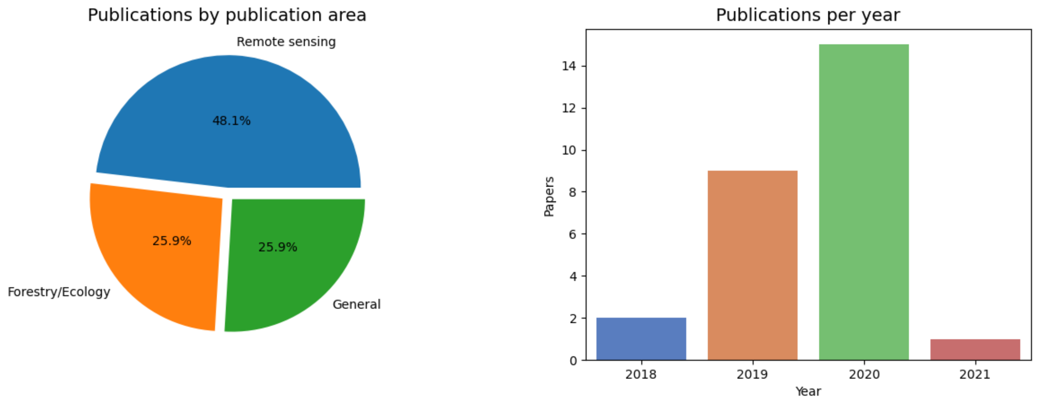
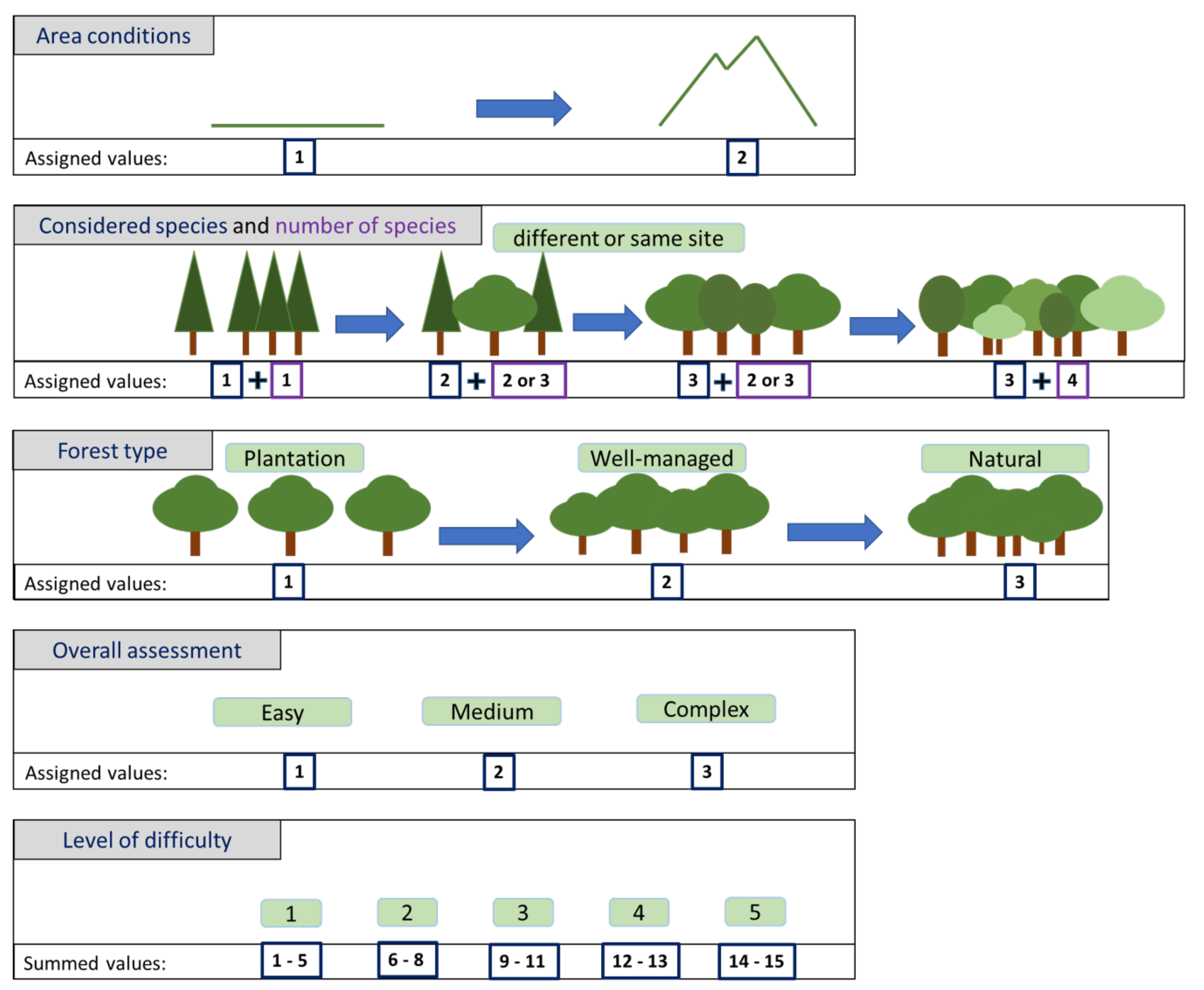
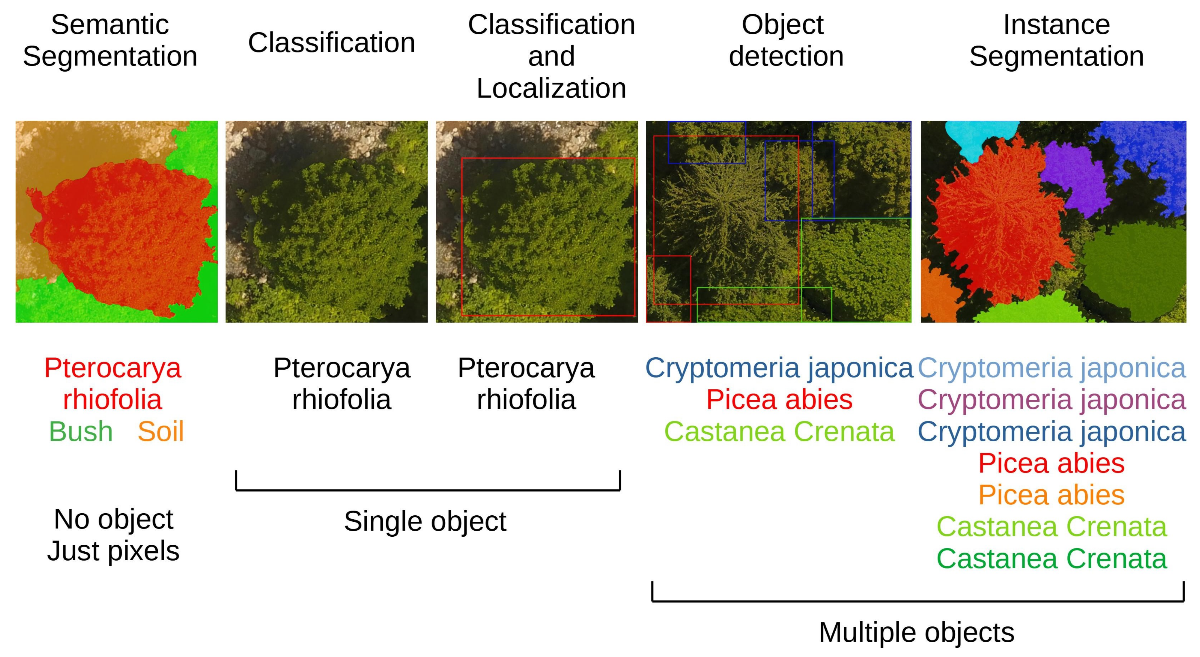
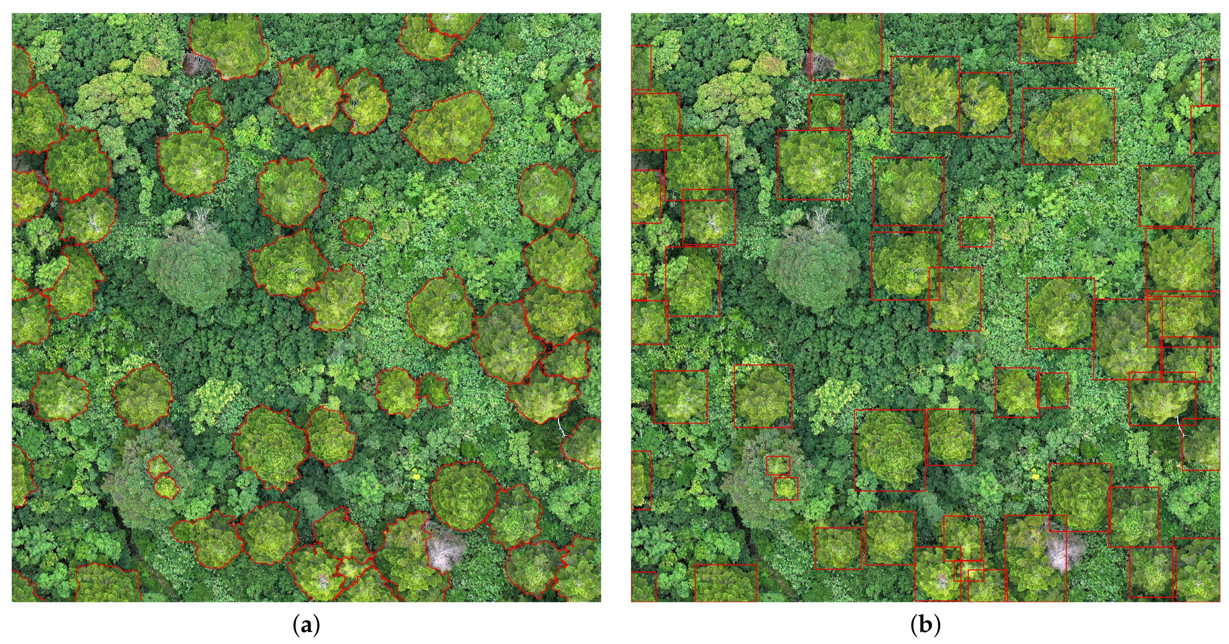
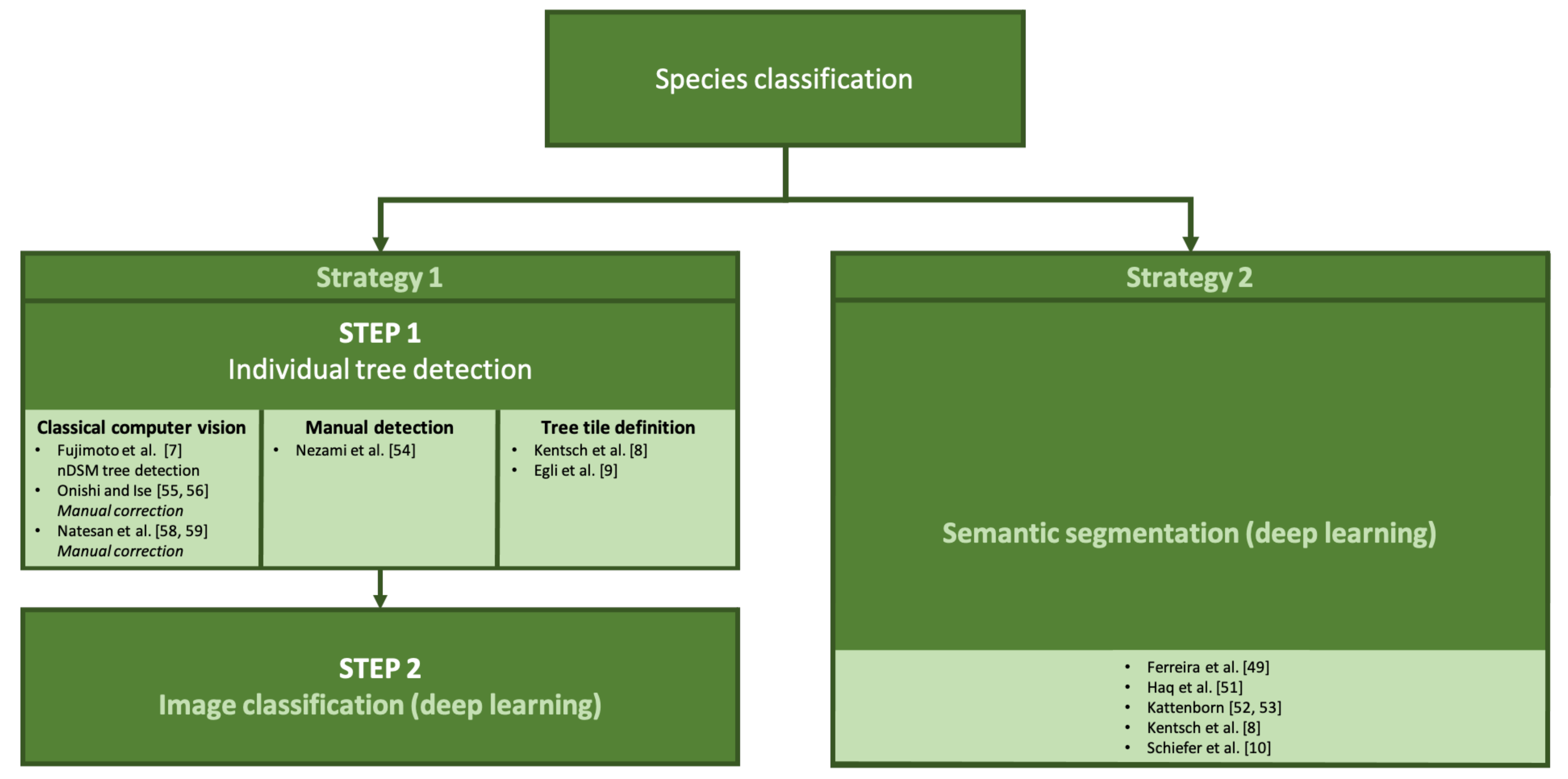
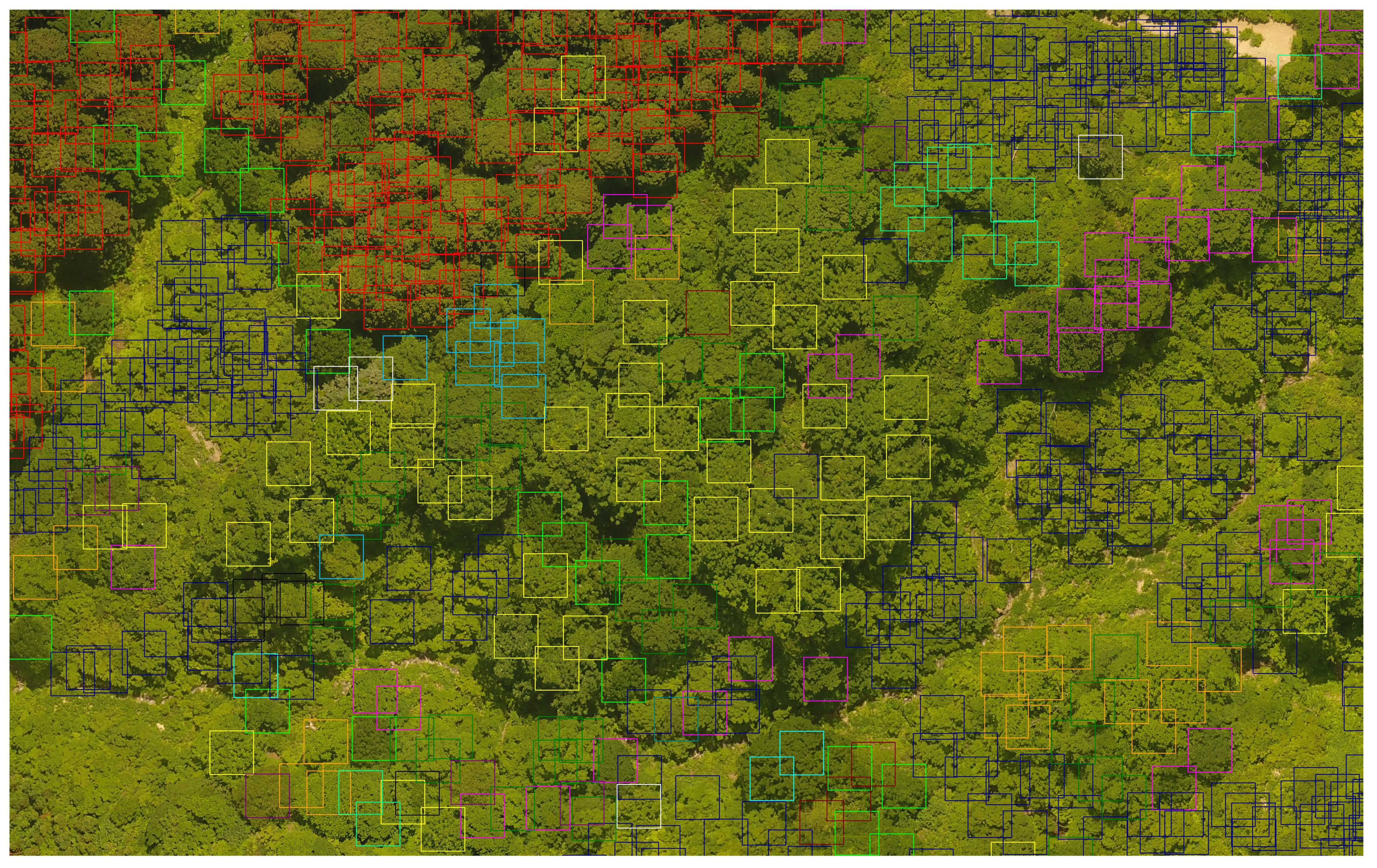
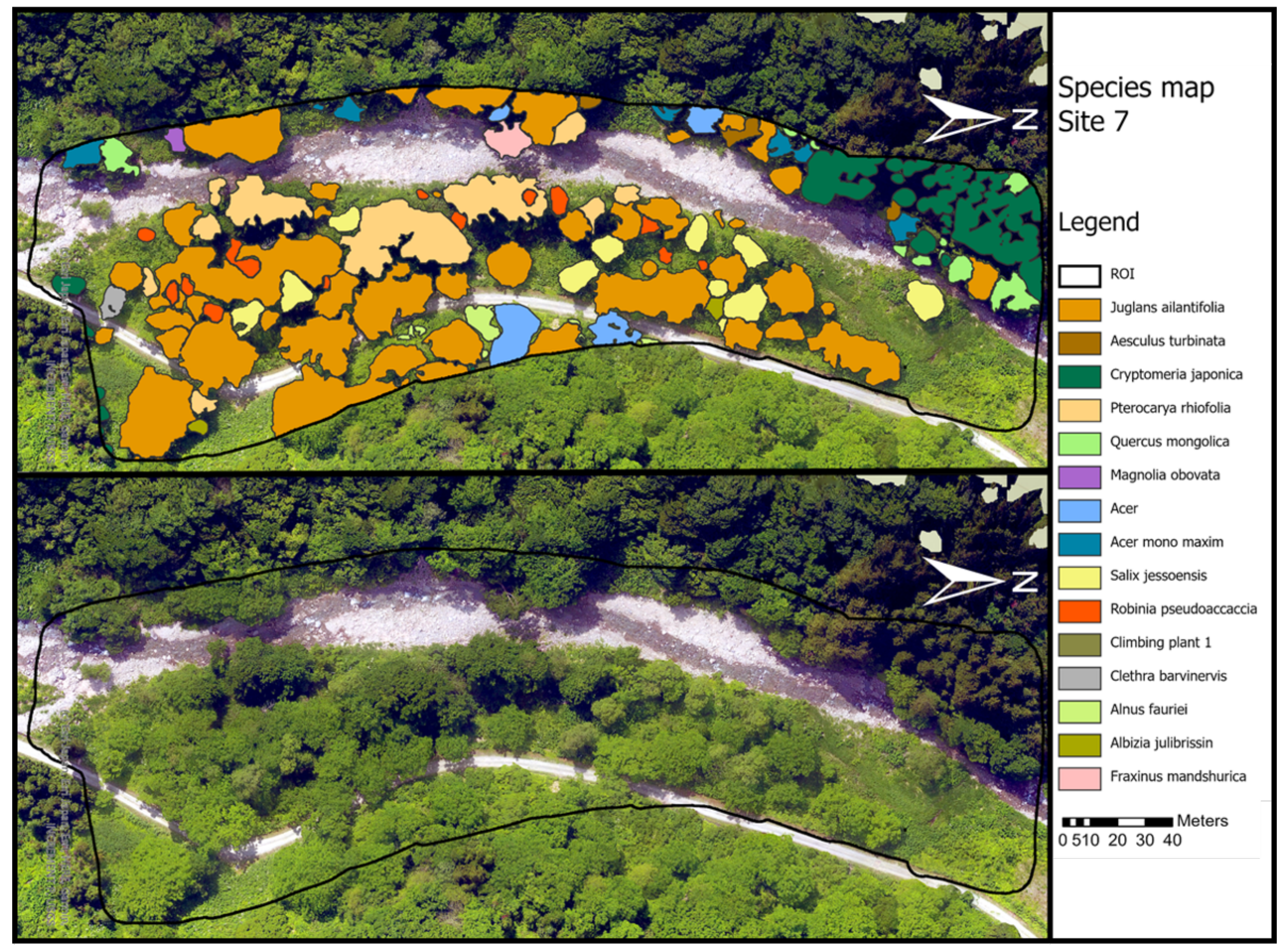
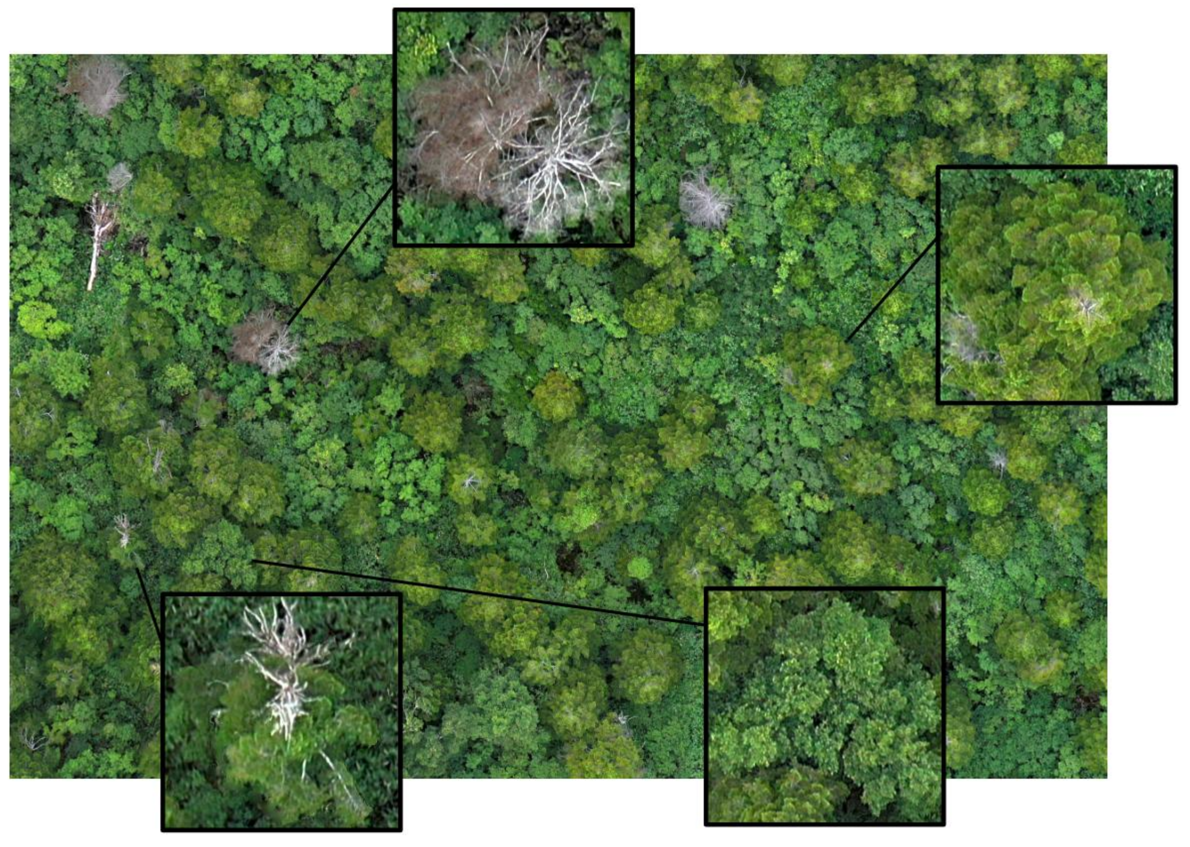
Table 1.
Summary of pre-processing and annotation software used in the reviewed papers.
| Refs. | 1st Author | Problem Solved | Type of Data | Pre-Processing Software | Annotation |
|---|---|---|---|---|---|
| [47] | López-Jiménez | Cactus detection | Single images | N/A | N/A |
| [48] | Fromm | Seedling detection | image tiles | N/A | LabelImg |
| [5] | Chadwick | Tree detection segmentation | Point cloud Orthomosaic | Pix4D LAStools | N/A |
| [6] | Ocer | Tree detection counting | Orthomosaic | ArcMap | Pix4D |
| [49] | Ferreira | Palm tree detection | Orthomosaic | Pix4D | QGIS |
| [7] | Fujimoto | Species Classification | 3D point cloud | Metashape Fusion | N/A |
| [50] | Morales | Palm tree Detection | original images | N/A | N/A |
| [51] | Haq | Species Classification | Orthomosaic | Pix4D | N/A |
| [52] | Kattenborn | Species Classification | Orthomosaic DEM | Metashape | GIS-based |
| [53] | Kattenborn | Species Classification | Orthomosaic DEM | Metashape | GIS-based |
| [8] | Kentsch | Species Classification | Orthomosaic | Metashape | GIMP |
| [54] | Nezami | Species Classification | Dense point clouds orthomosaic | Metashape, | N/A |
| [55,56] | Onishi | Species Classification | Orthomosaic DSM | Metashape, | eCognition ArcGIS |
| [57] | Lin | Species Classification | Single images | N/A | N/A |
| [58,59] | Natesan | Species Classification | Orthomosaic DSM | Metashape | Local Max. watershed |
| [10] | Schiefer | Species Classification | Orthomosaic DSM, nDSM | Metashape | ArcGIS |
| [60] | Barmpoutis | Tree Health classification | Orthomosaic | Metashape | N/A |
| [61] | Humer | Tree Health classification | Single images | N/A | GIMP |
| [62] | Deng | Dead tree detection | Orthomosaic | Metashape | LabelImg |
| [63] | Nguyen | Tree Health classification | Orthomosaic nDSM | Metashape | GIMP |
| [12] | Safonova | Tree Health classification | Orthomosaic, DEM | Metashape | N/A |
| [64] | Kim | Forest fire detecton | Single images | N/A | N/A |
| [11] | Tran | Post fire mapping | Orthomosaic | DroneDeploy | Labelme |
| [65] | Hossain | Smoke/flame/ detection | Single images | N/A | N/A |
| [66] | Zhao | Smoke/flame/ detection | Single images | N/A | N/A |
| [67] | Chen | Smoke/flame/ detection | Unprocessed Data Single images | N/A | N/A |
Table 2.
Summary of Papers reviewed addressing Individual tree detection using DL. N/A stands “Not Available”. Regarding the “Data Issues” column, the following notation is used: “Wrong Split” (WS), “Late Split” (LS), “validation set for testing” (VST), “dependent test set”(DTS) or “insufficient information” (IINF); see Section 3 for details.
| Ref. 1st Author | Problem Solved | Assessed Difficulty | Type of Data | Resolution | Amount of Data | DL Network | Data Issues |
|---|---|---|---|---|---|---|---|
| [47] López-Jiménez | Cactus detection (Single Label Classification) | 1 | Unprocessed images video patches | N/A | 16,136 + 5364 labelled images | LeNet 5 | IINF |
| [48] Fromm | Seedling detection | 2 | Unprocessed images | 0.3 cm | 3940 seedlings in two sites 25 m long 9415 512 × 512 tiles (multiple captures) | Faster R-CNN R-FCN, SSD | DTS |
| [5] Chadwick | Tree crown delineation | 2 | Point cloud Orthomosaic | 3 cm | 18 plots, 2.2–24.6 ha, tree stem density 1500–6800 | Mask R-CNN | DTS |
| [6] Ocer | Tree detection/counting | 2 | Orthomosaic | 4–6.5 cm | 2 flights, 2897 trees | Mask R-CNN | |
| [49] Ferreira | Palm tree detection (Species Classification) | 3 | Orthomosaic | 4 cm | 28 plots (250 × 150 m), 1423 images | DeepLabv3 | DTS |
Table 3.
Summary of Tree Species Classification papers reviewed. Regarding the “Data Issues” column, the following notation is used: “Wrong Split” (WS), “Late Split” (LS), “validation set for testing” (VST), “dependent test set”(DTS) or “insufficient information” (IINF); see Section 3 for details.
Table 3.
Summary of Tree Species Classification papers reviewed. Regarding the “Data Issues” column, the following notation is used: “Wrong Split” (WS), “Late Split” (LS), “validation set for testing” (VST), “dependent test set”(DTS) or “insufficient information” (IINF); see Section 3 for details.
| Ref. aUI | Problem Solved | Assessed Difficulty | Type of Data | Resolution | Amount of Data | DL Network | Data Issues |
|---|---|---|---|---|---|---|---|
| [7] Fujimoto | Species Classification (Grayscale image classification) | 2 | 3D point cloud DEM | 2.3–3.1 cm | 0.81 ha, 129+152 images | CNN | DTS |
| [50] Morales | Palm tree Detection (semantic segmentation) | 2 | unprocessed images | 1.4–2.5 cm | 4 flights, 25,248 patches | Deeplab v3+ | LS DTS |
| [51] Haq | Species Classification (semantic segmentation) | 2 | Orthomosaic? | 11.86 cm | 2040 km² area, 60 images | Autoencoder | IINF |
| [52] Kattenborn | Species Classification (semantic segmentation) | 2/3 | Orthomosaic, DEM | 3–5 cm | Site 1: 21–37 ha Site 2: 20–50 ha | CNN- UNet | LS VST |
| [53] Kattenborn | Species Mapping (Object Detection) | 2/3/3 | Orthomosaic, DEM | 5 cm, 3 cm, 3 cm | S1: 20–50 ha, 7 flights S2: 21–37, 8 flights S3: 4.3 ha, 3 flights | CNN | VST |
| [8] Kentsch | Species Classification Winter Mosaics and Invasive Species (multi-label image Classification) | 2/4 | Orthomosaic | 2.74 cm | 8 flights, 6 sites, 233–1000 images, 3–8 ha | ResNet50 | DTS * |
| [54] Nezami | Species Classification (single-label image Classification) | 3 | Dense point cloud orthomosaic | 5–10 cm | 8 flights, 3039 labelled data, 803 test data | 3D-CNN | DTS |
| [49] Ferreira | Palm tree detection/Classification (semantic segmentation) | 3 | Orthomosaic | 4 cm | 28 plots (250 × 150 m), 1423 images | DeepLabv3 | DTS |
| [55,56] Onishi | Species Classification (single-label image Classification) | 3 | Orthomosaic, DSM | 5–10 cm | 2 flights, 11 ha | CNN | DTS |
| [57] Lin | Species Classification (single-label image Classification) | 3 | unprocessed images | 0.47–1.76 cm | 50–65 images | Fourier Dense | VST |
| [9] Egli | Species Classification (single-label image Classification) | 4 | unprocessed images | 0.27–54.78 cm | 1556 images, 477 trees | lightweight CNN | |
| [58,59] Natesan | Species Classification (single-label image Classification) | 4 | Orthomosaic, DSM | 20 ha, 3 flights | VGG16, ResNet-50 DenseNet | DTS | |
| [10] Schiefer | Species Classification (semantic segmentation) | 4/5 | Orthomosaic, DSM DTM and nDSM | 1.35 cm resampled to 2 cm | 135 plots (100 × 100 m), 51 orthomosaics | CNN (UNet) | DTS ** |
Table 4.
Summary of forest fires studies reviewed. Regarding the “Data Issues” column, the following notation is used: “Wrong Split” (WS), “Late Split” (LS), “validation set for testing” (VST), “dependent test set” (DTS) or “insufficient information” (IINF), see Section 3 for details.
Table 4.
Summary of forest fires studies reviewed. Regarding the “Data Issues” column, the following notation is used: “Wrong Split” (WS), “Late Split” (LS), “validation set for testing” (VST), “dependent test set” (DTS) or “insufficient information” (IINF), see Section 3 for details.
| Ref. 1st Author | Assessed Difficulty | Problem Solved | Type of Data | Resolution | Amount of Data | DL Network | Data Issues |
|---|---|---|---|---|---|---|---|
| [64] Kim | 1 | Fire/not fire image classification | Single images | varying | 126,849 fire images 75,889 non fire | CNN | |
| [11] Tran | 2 | Burnt region coarse segmentation | Orthomosaic | N/A | 2 plots 43/44 images | UNet | |
| [65] Hossain | 1 | Fire/smoke coarse segmentation | Single images | varying | 460 images | YOLOv3 | IINF |
| [66] Zhao | 2 | Fire/not fire image classification | Single images | varying | 1500 images | CNN | |
| [67] Chen | 1 | Fire/smoke/normal image classification | Single images | varying | 2100 images | CNN | IINF |
Table 5.
Summary of Tree Health related papers reviewed. Regarding the “Data Issues” column, the following notation is used: “Wrong Split” (WS), “Late Split” (LS), “validation set for testing” (VST), “dependent test set” (DTS) or “insufficient information” (IINF), see Section 3 for details.
Table 5.
Summary of Tree Health related papers reviewed. Regarding the “Data Issues” column, the following notation is used: “Wrong Split” (WS), “Late Split” (LS), “validation set for testing” (VST), “dependent test set” (DTS) or “insufficient information” (IINF), see Section 3 for details.
| Ref. 1st Author | Problem Solved | Assessed Difficulty | Type of Data | Resolution | Amount of Data | DL Network | Data Issues |
|---|---|---|---|---|---|---|---|
| [60] Barmpoutis | Tree Health classification | 2 | Orthomosaic | N/A | 4 plots in 60 ha area, >1500 infected trees | Faster R-CNN Mask R-CNN | IINF |
| [61] Humer | Tree Health classification | 3 | unprocessed images | N/A | 35 images | UNet | VST |
| [62] Deng | Dead tree detection | 3 | Orthomosaic | N/A | 1.7952 km, 340 data points, augmented 1700 | Faster R-CNN | LS DTS |
| [63] Nguyen | Tree Health classification | 4 | Orthomosaic | 1.45–2.6 cms/pixel | 18 Ha, 9 Orthomosaics | ResNet | |
| [12] Safonova | Tree Health classification | 5 | Orthomosaic | 5–10 cms/pixel | 1200 images, 4 Orthomosaics | Custom CNN |
Publisher’s Note: MDPI stays neutral with regard to jurisdictional claims in published maps and institutional affiliations. |
© 2021 by the authors. Licensee MDPI, Basel, Switzerland. This article is an open access article distributed under the terms and conditions of the Creative Commons Attribution (CC BY) license (https://creativecommons.org/licenses/by/4.0/).
Share and Cite
MDPI and ACS Style
Diez, Y.; Kentsch, S.; Fukuda, M.; Caceres, M.L.L.; Moritake, K.; Cabezas, M. Deep Learning in Forestry Using UAV-Acquired RGB Data: A Practical Review. Remote Sens. 2021, 13, 2837. https://0-doi-org.brum.beds.ac.uk/10.3390/rs13142837
AMA Style
Diez Y, Kentsch S, Fukuda M, Caceres MLL, Moritake K, Cabezas M. Deep Learning in Forestry Using UAV-Acquired RGB Data: A Practical Review. Remote Sensing. 2021; 13(14):2837. https://0-doi-org.brum.beds.ac.uk/10.3390/rs13142837
Chicago/Turabian StyleDiez, Yago, Sarah Kentsch, Motohisa Fukuda, Maximo Larry Lopez Caceres, Koma Moritake, and Mariano Cabezas. 2021. "Deep Learning in Forestry Using UAV-Acquired RGB Data: A Practical Review" Remote Sensing 13, no. 14: 2837. https://0-doi-org.brum.beds.ac.uk/10.3390/rs13142837
Note that from the first issue of 2016, this journal uses article numbers instead of page numbers. See further details here.