
Shallow Shear-Wave Velocity Structure beneath the West Lake Area in Hangzhou, China, from Ambient-Noise Tomography


Key Laboratory of Geoscience Big Data and Deep Resource of Zhejiang Province, School of Earth Sciences, Zhejiang University, Hangzhou 310027, China
*
Author to whom correspondence should be addressed.
Remote Sens. 2021, 13(14), 2845; https://0-doi-org.brum.beds.ac.uk/10.3390/rs13142845
Submission received: 25 May 2021
/
Revised: 30 June 2021
/
Accepted: 14 July 2021
/
Published: 20 July 2021
(This article belongs to the Section Remote Sensing in Geology, Geomorphology and Hydrology)
Abstract
:Urban geophysical exploration plays an important role in the sustainable development of and the mitigation of geological hazards in metropolitan areas. However, it is not suitable to implement active seismic methods in densely populated urban areas. The rapidly developing ambient-noise tomography (ANT) method is a promising technique for imaging the near-surface seismic velocity structure. We selected the West Lake area of the city of Hangzhou as a case study to probe the shallow subsurface shear-wave velocity (Vs) structure using ANT. We conducted seismic interferometry on the ambient-noise data recorded by 28 seismograph stations during a time period of 17 days. Fundamental-mode Rayleigh-wave group- and phase-velocity dispersion data were measured from cross-correlation functions and then inverted for a 3D Vs model of the uppermost 1 km that covers an area of about 7 km × 8 km. The tomographic results reveal two prominent anomalies, with high velocities in the southwest and low velocities in the northeast. The fast anomaly corresponds to the presence of limestone and sandstone, whereas the slow anomaly is due to the relatively low-velocity rhyolite and volcanic tuff in the area. The boundary between the two anomalies lies to the NE of an NW–SE trending fault, indicating that the fault dips toward the NE. In addition, the pronounced low-velocity anomalies appear under the Baoshi mountain, likely due to the thick rhyolite and volcanic tuff beneath the extinct volcano. Our results correlate well with regional geological features and suggest that ANT could be a promising technique for facilitating the exploration of urban underground space.
1. Introduction
Hangzhou is the capital city of Zhejiang province, southeastern China, with a population of over 9.8 million. The area around the West Lake in Hangzhou, a tourist attraction well-known nationwide, has suffered from tens of geological hazards, such as landslides and rockfall, which are in connection with the mountainous environment and complex geostructures such as the West Lake synclinorium. In addition, widespread unconsolidated sediments in the city may increase earthquake risk by amplifying the ground motion from potential adjacent earthquakes. Hence, there is an urgent demand to conduct urban geophysical surveys in this area, which are necessary for the related exploitation of underground resources and the mitigation of geological hazards. However, active (controlled-source) seismic methods are not suitable due to environmental issues in the urban area. To this end, we employed an environmentally friendly imaging technique, that is, ambient-noise tomography (ANT), to image the shallow shear-wave velocity (Vs) structure beneath the West Lake area.
ANT is based on the principle of generating empirical Green’s functions (EGFs) by cross-correlating ambient noise recorded at different receivers [1,2,3,4], which are in turn used for tomography. Previous theoretical work [1,2,3,4] showed that under the assumption of a homogenous source distribution, the EGF between stations A and B () can be expressed as
where represents the correlation functions. Campillo and Paul [5] first demonstrated that EGFs between two receivers can be retrieved by cross-correlation of the seismic coda waves. Then, Shapiro and Campillo [6] successfully extracted Rayleigh waves by correlating ambient seismic noise. Shapiro et al. [7] performed the first ambient-noise Rayleigh-wave tomography in South California. A large number of subsequent applications of ANT have been focused on continental- or regional-scale crustal structure [8,9,10,11,12,13]. Recently, an increasing number of applications have been focused on local-scale shallow structure [14,15,16,17].
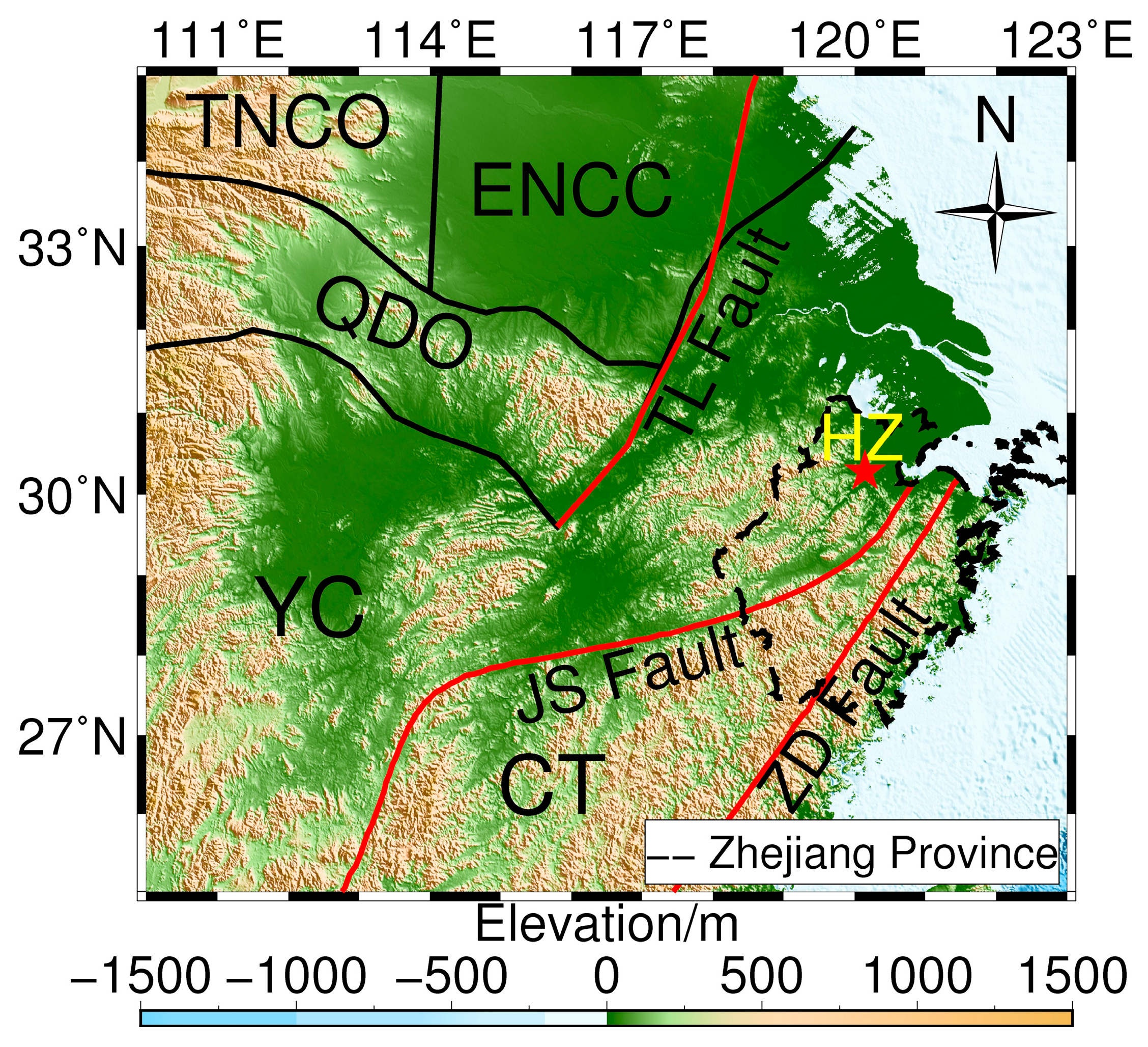
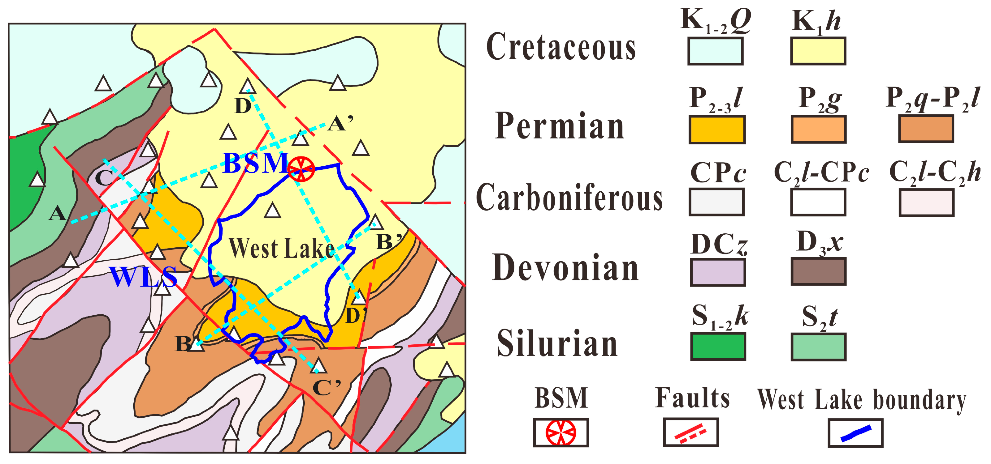
The aforementioned studies pave the way for the application of ANT in urban geophysical exploration. We selected the West Lake area as a case study to image the shallow Vs structure and to verify the applicability of ambient-noise tomography in urban underground space exploration. Our study region (Figure 1) is to the northwest of the Jiangshan–Shaoxing fault zone, the suture between the Yangtze Craton and the Cathaysia Terrane in the South China Block. The Cathaysia Terrane was subducted under the Yangtze Craton during the Neoproterozoic [18,19]. Subsequently, the Mesozoic subduction of the paleo-Pacific plate beneath the Eurasian plate led to the formation of several NE–SW trending faults, folds, and volcanos, which form the current tectonic frameworks in Hangzhou [20]. The Baoshi mountain (BSM in Figure 2) is an extinct volcano and once erupted tuff that covered the northeastern WLS during the early Cretaceous. During the neotectonics, the northeastern part of the West Lake synclinorium (WLS) experienced significant subsidence while the southwestern WLS was uplifted [21,22]. From the geological map of the West Lake area (Figure 2), it can be seen that the study area is mainly composed of Paleozoic sandstone and limestone with Cretaceous rhyolite and volcanic tuff in the northeastern part.
2. Data and Method
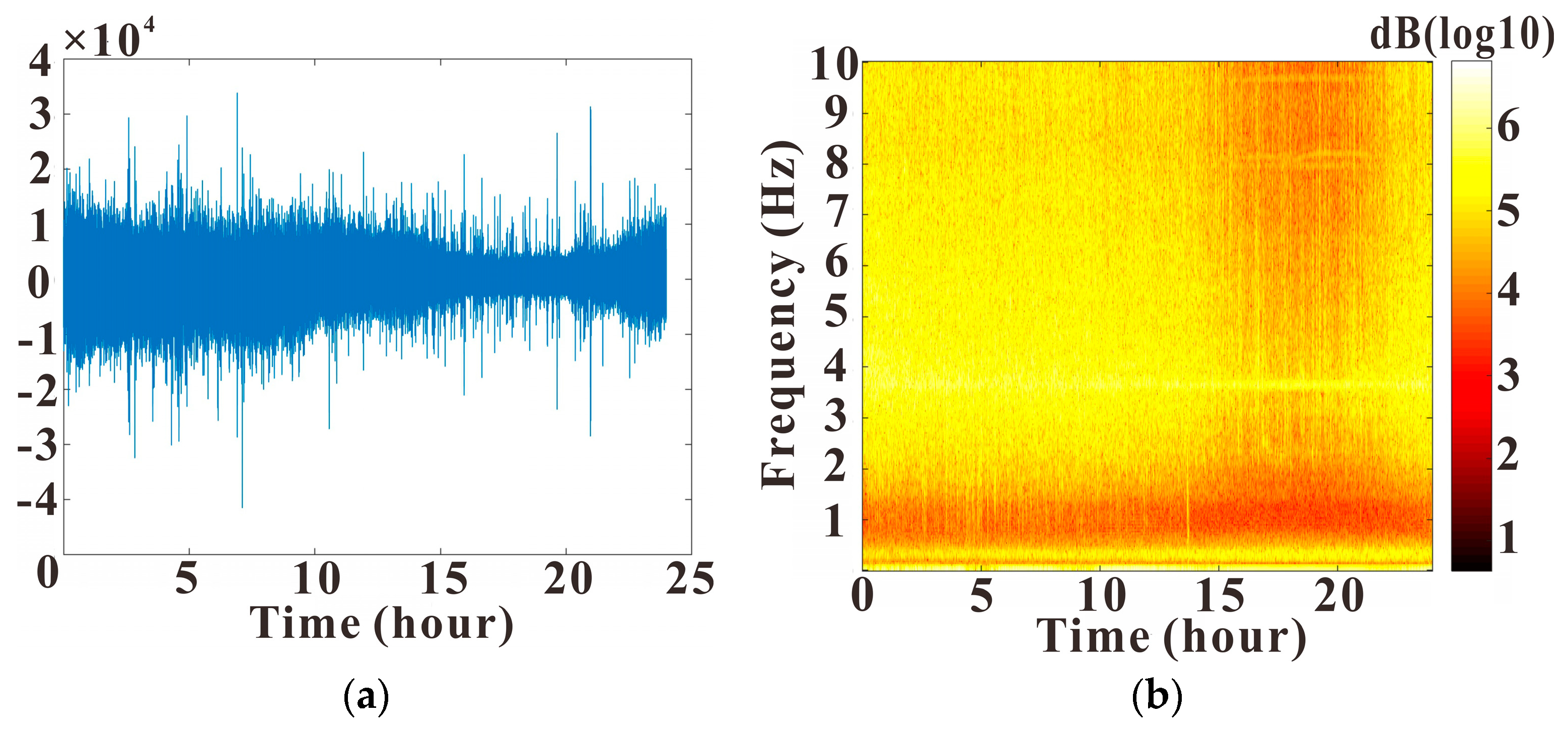
We deployed 28 broadband seismograph stations (equipped with Trillium Horizon 120 seismometer and Centaur digitizer) in the West Lake area to acquire ambient-noise data with a sampling rate of 200 Hz and an average interstation spacing of ~0.5–1 km (Figure 2). Data acquisition lasted for 17 days, from 29 July to 14 August 2018. The study region covers an area of 7 km × 8 km. Figure 3a,b show a one-day vertical-component waveform recorded by station WL.B04 (Figure 2) and its spectrogram, respectively. The amplitude of the spectrogram is higher during the daytime than during the night, which is due to the influence of anthropogenic activities.
Only vertical-component data were processed to obtain Rayleigh-wave EGFs using procedures similar to those documented in Reference [23]. First, we truncated the data into hour-long segments and decimated the recordings at a sampling rate of 50 Hz. We removed the mean and trend from the data. Then, the data were bandpass-filtered between 0.2 and 5 s periods. Both temporal and spectral normalizations were applied before cross-correlation to reduce the influence of earthquakes and non-stationary noise energy. Since running-absolute-mean normalization of the recordings can lead to faster convergence of noise cross-correlation functions (NCFs) [24], we implemented running-absolute-mean normalization instead of 1-bit normalization for the purpose of temporal normalization. Finally, cross-correlation was performed on hour-long recordings for each station pair with lag times ranging from −30 s to 30 s. These hourly results were stacked to obtain the final NCFs corresponding to the whole recording duration for each station pair. In total, we obtained 378 NCFs.
Conventional linear stacking and time-frequency domain phase-weighted stacking (tf-PWS) techniques were compared to increase the signal-to-noise ratio (SNR) of NCFs. Tf-PWS calculates the phase coherence coefficients and downweights the inconsistent signals in the linear stacked NCFs [25,26]. Figure 4a,b show the NCFs for one station pair recovered by two stacking schemes, respectively, illustrating the considerable increase in the SNR by the tf-PWS. More NCFs with higher SNRs can be obtained from the tf-PWS method than the linear stacking method (Figure 4c,d). Hence, NCFs constructed from the tf-PWS method were used for later processing. As seen in Figure 4c,d, the coherent Rayleigh waves elucidate an apparent velocity of approximately 2 km/s.
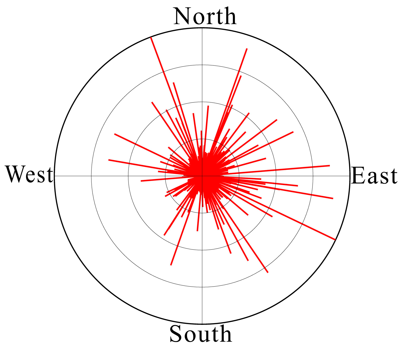
Since the uneven distribution of noise energy would distort the NCFs and affect the reliability of dispersion measurements [27], we calculated the SNR for both acausal and causal components in each NCF as a proxy to identify the azimuth dependence of noise energy. SNR is defined by the ratio of the absolute maximum amplitude within the signal window and the root mean square value in the noise window (−30 to −15 s and 15 to 30 s). The analysis of noise directionality is similar to the technique adopted by Yang and Ritzwoller [28], in which the strength of directional noise energy from two opposite azimuths was estimated by the SNR values. The azimuthal distribution of SNRs for both acausal and causal components of all NCFs is shown in Figure 5. We normalized the SNRs by the maximum SNR value and found that approximately equal power of noise energy arrived from variant directions, indicating that the noise source is nearly homogeneous.
3. Results
3.1. Rayleigh-Wave Dispersion Curve Measurement
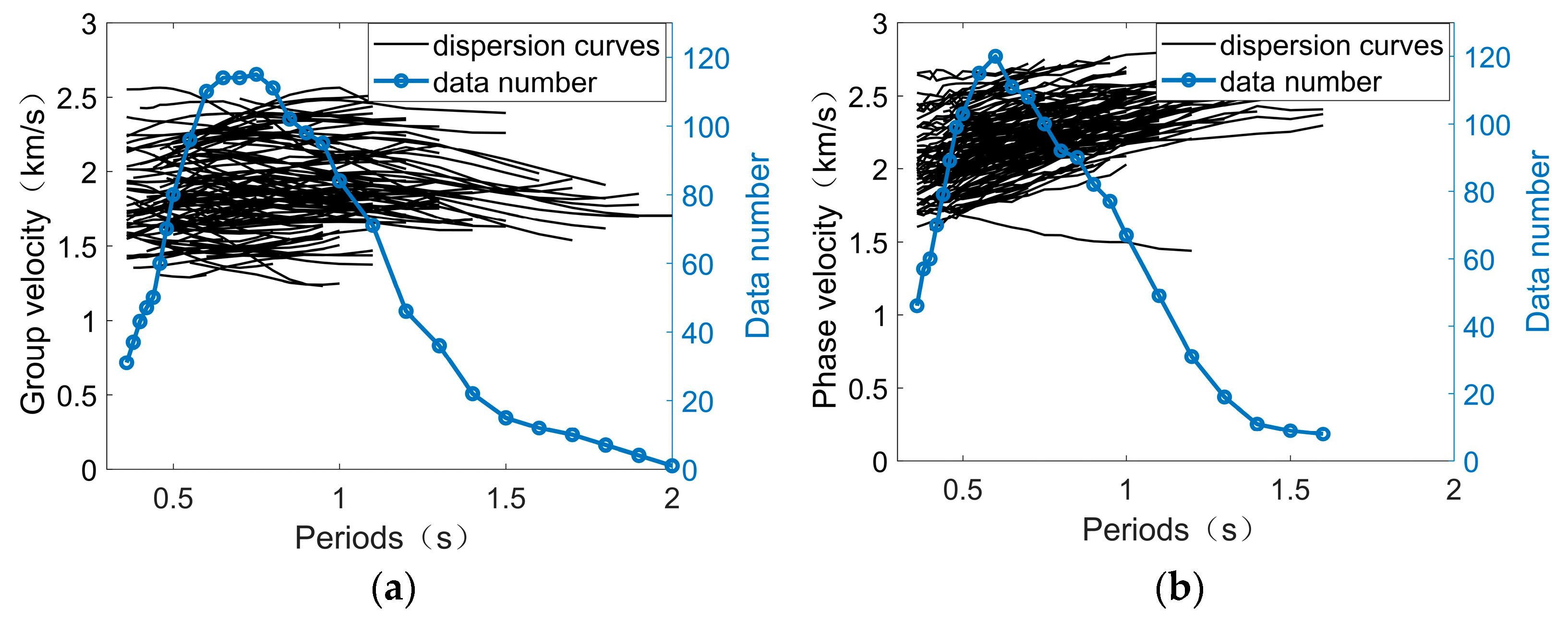
We stacked the causal and acausal parts of the NCFs linearly to form the symmetric component of NCFs. Then, the dispersion curve was extracted from every symmetric NCF using the multiple filter analysis package in Computer Program in Seismology (CPS) [29,30]. We checked the quality of every symmetric NCF carefully and chose dispersion curves manually. Two selection criteria were applied to avoid biased dispersion measurements. First, interstation distance should be at least 1.5 times the wavelength to satisfy the surface-wave far-field approximation condition. Second, the SNR of NCFs should be greater than 10 to retain the most reliable measurements. The extracted group- and phase-velocity dispersion curves for the fundamental-mode Rayleigh wave in the period range from 0.35 s to 2 s are shown in Figure 6a,b. A total of 132 group- and 142 phase-velocity dispersion lines were extracted. The group velocity varies from 1.3 km/s to 2.7 km/s and the phase velocity from 1.5 km/s to 2.7 km/s at a period of 0.4 s. The obvious velocity variations in the group and phase velocities indicate strong velocity heterogeneities in the research area.
3.2. Construction of 3D Vs Model
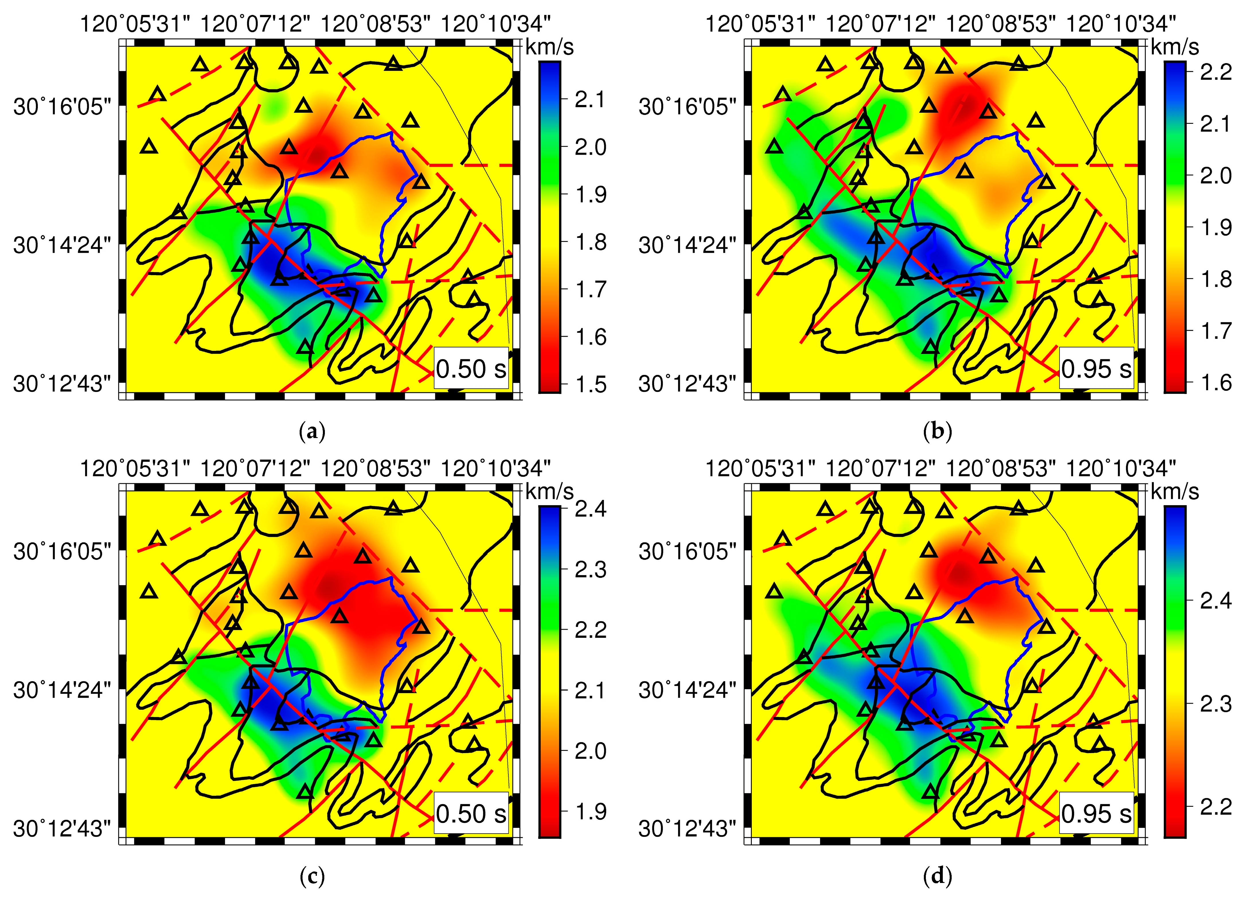
A two-step inversion scheme was implemented to obtain the 3D Vs model. We first inverted the group- and phase-velocity dispersion measurements for 2D group- and phase-velocity maps, respectively, on a 0.003° × 0.003° grid at different periods using a non-linear tomographic technique [31]. For the forward problem, a fast-marching method [32,33] was employed to calculate the travel-time field by solving the grid-based Eikonal equation through a wave-front tracking method, and then the travel-time gradient was calculated to determine the ray paths between station pairs. The final model was solved by an iterative subspace inversion scheme [34]. The optimum damping and smoothing weights were obtained from the standard trade-off curves for travel-time residuals and model roughnesses. We also performed over-smoothed tomographic inversions and rejected dispersion measurements with residuals greater than 2.5 standard deviations from the mean residual. The resulting group-velocity maps were plotted in the period range of 0.46 s to 1.1 s and phase-velocity maps from 0.40 s to 0.95 s (Figure 7).
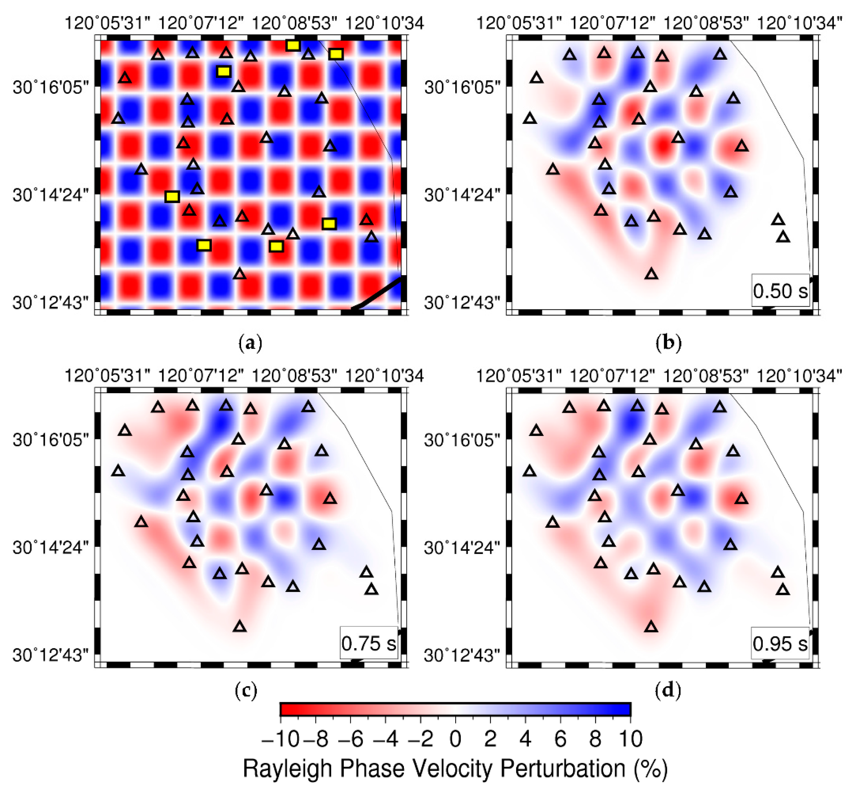
We further evaluated the spatial resolution of our model through synthetic checkerboard tests. The synthetic initial model consists of high- and low-velocity checkers with the maximum velocity perturbation of 10% relative to the average velocity. The checkerboard size was three times the grid size, and randomly distributed noise was added to the synthetic data. Here, the randomly distributed noise level was set to be 1% of the theoretical travel time. The recovered phase-velocity checkerboards at three specific periods are shown in Figure 8, suggesting that the tomographic results are capable of resolving structures with a lateral resolution of about 1 km × 1 km.
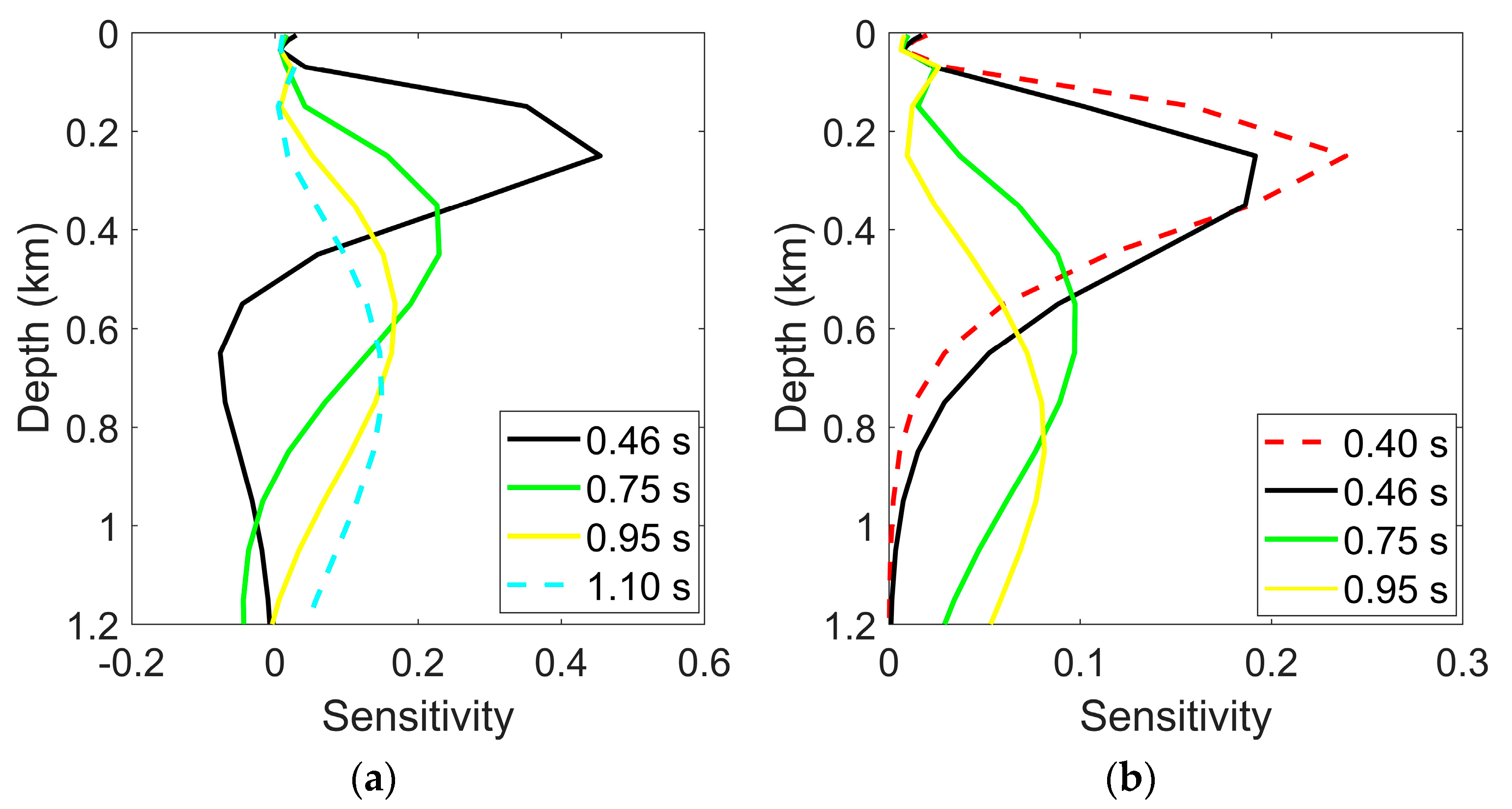
Rayleigh-wave group- and phase-velocity dispersion curves at every grid point were combined to jointly invert for the isotropic 1D Vs profile using a linearized procedure [30]. The average velocity for the uppermost 40 m from the borehole data (yellow rectangles in Figure 8a) and the deep crustal Vs model from Bao et al. [10] were integrated to generate the initial model with a layer thickness of 100 m. Surface waves at different periods are sensitive to structures at different depth ranges. The peak of the sensitivity kernel for the Rayleigh wave is around one-third of its wavelength. For a given period, Rayleigh-wave group velocity is sensitive to shallower structures than phase velocity. The inverted 1D Vs model at one grid point is used to calculate the sensitivity kernel using CPS package [30]. From the sensitivity kernels shown in Figure 9, our dataset can effectively constrain the Vs structure down to a depth of ~1 km.
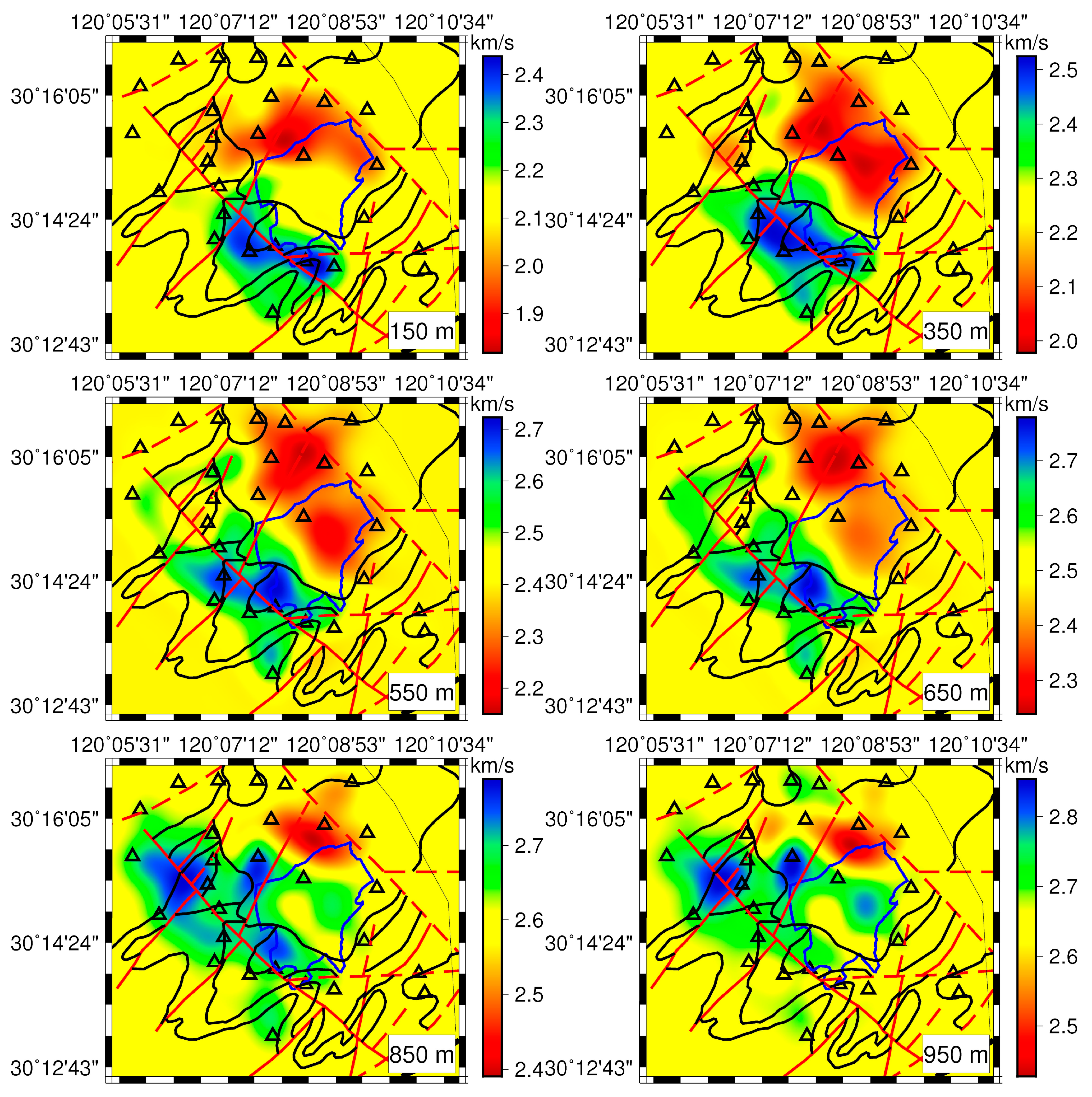
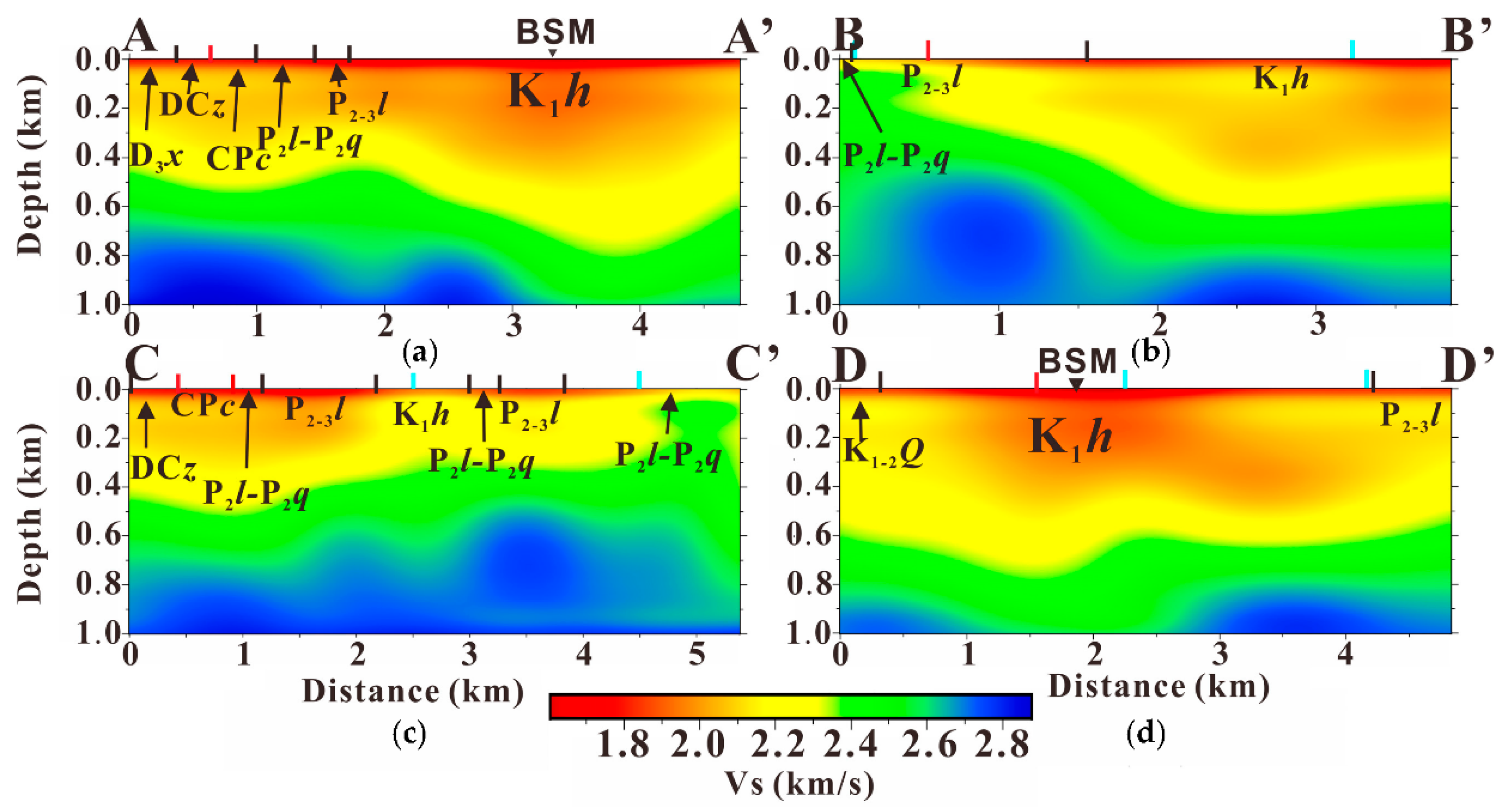
We assembled all the 1D Vs models at each grid point to construct the final 3D Vs model. Several representative horizontal slices were plotted in Figure 10, showing an obvious bimodal distribution of Vs in the area as observed in Rayleigh-wave group- and phase-velocity maps (Figure 7): high-velocity anomalies in the southwest and low-velocity anomalies in the northeast. The fast anomalies mainly occur in the southwestern WLS, whereas the slow anomalies in the northeast generally correspond to the BSM and the West Lake region. The boundary separating the two anomalies lies to the NE of a NW–SE trending fault, suggesting that the fault dips towards NE. Furthermore, four velocity profiles in Figure 11 traversing the main geological structures (Figure 2) were plotted to display the lateral velocity variations. It is noticeable again that the boundary between the low-velocity structure in the northeast and the high-velocity structure in the southwest dips toward NE (AA’ and BB’ profiles). As shown in profiles AA’ and DD’, relatively thick low-velocity layers appear beneath the BSM.
4. Discussion
In this study, using the 17-day continuous ambient-noise data, we extracted high-SNR Rayleigh waves within the period range of 0.35–2 s, which were inverted to constrain the subsurface Vs structure to ~1 km depth. Higher- and lower-frequency surface waves with high SNRs cannot be recovered, likely due to the limitation of inter-station spacing and high attenuation of the shallow medium. Generally speaking, we can obtain higher.
Frequency surface waves with shorter station-pair distance and vice versa. For example, using data from the extremely dense seismic array in Long Beach, California, with an average inter-station spacing of ~100 m, Lin et al. [14] extracted Rayleigh waves with frequencies of up to 4 Hz, which can improve the resolution of the near-surface structure.
From the sensitivity kernels of the extracted Rayleigh waves (Figure 9), we can see that our data are highly sensitive to the subsurface structure below 100 m depth. Thus, we suggest that the shallow structures located above 50 m depth are not the likely cause of the imaged velocity variations. Hence, the predominant velocity anomalies are mainly associated with the variations in the underlying bedrock. From the geological map (Figure 2), the western WLS comprises two synclines and is mainly composed of Paleozoic sandstone and limestone, while the subsided northeastern WLS is covered by the Cretaceous rhyolite and tuff. The limestone and sandstone have higher shear velocity (about 2.0–3.3 km/s) than the rhyolite and tuff (about 1.5–2.4 km/s). Thus, our tomographic models correlate well with the known geological features. The high-velocity anomaly in the southwest corresponds to the sandstone and limestone, while the slow anomaly in the northeast is related to the low-velocity rhyolite and volcanic tuff. It can be seen that the low-velocity area shrinks at greater depths and appears only beneath the BSM at depths of 850–950 m, likely due to the thick rhyolite and tuff beneath the extinct volcano.
Based on the correlation between our tomographic model and the geologic features, we further demonstrate here the applicability of ambient-noise tomography in delineating the shallow Vs structure in urban areas for facilitating the exploration of urban underground structures. In addition, we also reveal the geometry of a regional fault. The structural variations across other faults have also been illuminated by previous studies, such as the Newport–Inglewood fault in Southern California [14] and the Shushan fault in the city of Hefei [15], emphasizing the promising future of ANT in studying the fault zone structure and for seismic hazard and risk assessment, since the ground motion of an earthquake is significantly influenced by the shallow Vs structure. With the potential of extracting body waves [35], more detailed structures of the shallow crust could also be resolved by ambient-noise interferometry.
5. Conclusions
In this study, we applied the environmentally friendly ANT method to investigate the shallow Vs structure surrounding the West Lake. The SNRs of NCFs were increased by the tf-PWS method. We measured fundamental-mode Rayleigh-wave dispersion curves within 0.35–2 s period band. A two-step inversion scheme was implemented to construct a 3D Vs model with a horizontal resolution of about 1 km × 1 km, which correlates well with regional geological features. Our tomographic model illustrates two prominent anomalies with high velocities in the southwest and low velocities in the northeast. The former anomaly corresponds to the presence of limestone and sandstone, whereas the latter is due to the relatively low-velocity rhyolite and volcanic tuff in that region. In addition, the boundary between the two anomalies lies to the NE of an NW–SE trending fault, suggesting that the fault dips toward NE. The Baoshi mountain is underlain by a thick, pronounced low-velocity structure, likely due to the thick rhyolite and volcanic tuff beneath the extinct volcano. Our results further suggest that ambient-noise tomography is a promising technique in facilitating the exploration of urban underground space and seismic hazard and risk assessment.
Author Contributions
Writing—original draft preparation, Z.C.; writing—review and editing, X.B.; methodology, Z.C. and X.B.; investigation, Z.C., X.B., and W.Y.; software, Z.C. and X.B.; visualization, Z.C.; data curation, X.B.; supervision, X.B.; funding acquisition, X.B. and W.Y. All authors have read and agreed to the published version of the manuscript.
Funding
This research was funded by the National Natural Science Foundation of China, grant number 41774045, and the Zhejiang Province Academician Industry Science and Technology Strategy Consulting Project, grant number 41574111.
Institutional Review Board Statement
Not applicable.
Informed Consent Statement
Not applicable.
Data Availability Statement
The ambient-noise data in current research are conserved by Xuewei Bao. Anyone who wants to use the data can send an email to [email protected].
Conflicts of Interest
The authors declare no conflict of interest.
References
- Wapenaar, K.; Fokkema, J. Green’s function representations for seismic interferometry. Geophysics 2006, 71, SI33–SI46. [Google Scholar] [CrossRef]
- Lobkis, O.I.; Weaver, R.L. On the emergence of the green’s function in the correlations of a diffuse field. J. Acoust. Soc. Am. 2001, 110, 3011–3017. [Google Scholar] [CrossRef] [Green Version]
- Snieder, R. Extracting the green’s function from the correlation of coda waves: A derivation based on stationary phase. Phys. Rev. E Stat. Nonlinear Soft Matter Phys. 2004, 69, 046610. [Google Scholar] [CrossRef] [Green Version]
- Roux, P.; Sabra, K.G.; Kuperman, W.A.; Roux, A. Ambient noise cross correlation in free space: Theoretical approach. J. Acoust. Soc. Am. 2005, 117, 79–84. [Google Scholar] [CrossRef] [Green Version]
- Campillo, M.; Paul, A. Long-range correlations in the diffuse seismic coda. Science 2003, 299, 547–549. [Google Scholar] [CrossRef] [PubMed] [Green Version]
- Shapiro, N.M.; Campillo, M. Emergence of broadband rayleigh waves from correlations of the ambient seismic noise. Geophys. Res. Lett. 2004, 31. [Google Scholar] [CrossRef] [Green Version]
- Shapiro, N.M.; Campillo, M.; Stehly, L.; Ritzwoller, M.H. High-resolution surface-wave tomography from ambient seismic noise. Science 2005, 307, 1615–1618. [Google Scholar] [CrossRef] [Green Version]
- Yao, H.; van der Hilst, R.D. Analysis of ambient noise energy distribution and phase velocity bias in ambient noise tomography, with application to SE Tibet. Geophys. J. Int. 2009, 179, 1113–1132. [Google Scholar] [CrossRef] [Green Version]
- Mottaghi, A.A.; Rezapour, M.; Tibuleac, I. Ambient noise rayleigh wave shallow tomography in the tehran region, Central Alborz, Iran. Seismol. Res. Lett. 2012, 83, 498–504. [Google Scholar] [CrossRef]
- Bao, X.; Song, X.; Li, J. High-resolution lithospheric structure beneath mainland China from ambient noise and earthquake surface-wave tomography. Earth Planet. Sci. Lett. 2015, 417, 132–141. [Google Scholar] [CrossRef]
- Spica, Z.; Perton, M.; Calò, M.; Legrand, D.; Córdoba-Montiel, F.; Iglesias, A. 3-D shear wave velocity model of Mexico and South US: Bridging seismic networks with ambient noise cross-correlations (C1) and correlation of coda of correlations (C3). Geophys. J. Int. 2016, 206, 1795–1813. [Google Scholar] [CrossRef] [Green Version]
- Yeck, W.L.; Sheehan, A.F.; Stachnik, J.C.; Lin, F.-C. Offshore rayleigh group velocity observations of the South Island, New Zealand, from ambient noise data. Geophys. J. Int. 2017, 209, 827–841. [Google Scholar] [CrossRef]
- Ku, C.-S.; Kuo, Y.-T.; Chao, W.-A.; You, S.-H.; Huang, B.-S.; Chen, Y.-G.; Taylor, F.W.; Wu, Y.-M. A first-layered crustal velocity model for the western solomon islands: Inversion of the measured group velocity of surface waves using ambient noise. Seismol. Res. Lett. 2018, 89, 2274–2283. [Google Scholar] [CrossRef]
- Lin, F.-C.; Li, D.; Clayton, R.W.; Hollis, D. High-resolution 3D shallow crustal structure in Long Beach, California: Application of ambient noise tomography on a dense seismic array. Geophysics 2013, 78, Q45–Q56. [Google Scholar] [CrossRef] [Green Version]
- Li, C.; Yao, H.; Fang, H.; Huang, X.; Wan, K.; Zhang, H.; Wang, K. 3D Near-surface shear-wave velocity structure from ambient-noise tomography and borehole data in the Hefei urban area, China. Seismol. Res. Lett. 2016, 87, 882–892. [Google Scholar] [CrossRef] [Green Version]
- Pan, Y.; Xia, J.; Xu, Y.; Xu, Z.; Cheng, F.; Xu, H.; Gao, L. Delineating shallow S-wave velocity structure using multiple ambient-noise surface-wave methods: An example from Western Junggar, China. Bull. Seismol. Soc. Am. 2016, 106, 327–336. [Google Scholar] [CrossRef]
- Czarny, R.; Pilecki, Z.; Nakata, N.; Pilecka, E.; Krawiec, K.; Harba, P.; Barnaś, M. 3D S-wave velocity imaging of a subsurface disturbed by mining using ambient seismic noise. Eng. Geol. 2019, 251, 115–127. [Google Scholar] [CrossRef]
- Charvet, J.; Shu, L.; Shi, Y.; Guo, L.; Faure, M. The building of South China: Collision of Yangzi and Cathaysia blocks, problems and tentative answers. J. Southeast Asian Earth Sci. 1996, 13, 223–235. [Google Scholar] [CrossRef]
- Xu, X.; Li, Y.; Tang, S.; Xue, D.; Zhang, Z. Neoproterozoic to early paleozoic polyorogenic deformation in the southeastern margin of the Yangtze block: Constraints from structural analysis and 40Ar/39Ar geochronology. J. Asian Earth Sci. 2015, 98, 141–151. [Google Scholar] [CrossRef]
- Lu, P. The Research of Sedimentary Structure and Spatial Distribution of the Quaternary Systerm of Hangzhou; Zhejiang University: Zhejiang, China, 2008. (In Chinese) [Google Scholar]
- Chen, Z.; Bao, C. The Evolution of West Lake in Hangzhou. Available online: http://cpfd.cnki.com.cn/Article/CPFDTOTAL-LYDZ199810001030.htm (accessed on 25 May 2021). (In Chinese).
- Chen, Y.; Hu, G.; Tong, L. Investigation on seismic effect of engineering geological structures in Hangzhou City. Geotechn. Investig. Surv. 2009, 14, 538–543. (In Chinese) [Google Scholar]
- Bensen, G.D.; Ritzwoller, M.H.; Barmin, M.P.; Levshin, A.L.; Lin, F.; Moschetti, M.P.; Shapiro, N.M.; Yang, Y. Processing seismic ambient noise data to obtain reliable broad-band surface wave dispersion measurements. Geophys. J. Int. 2007, 169, 1239–1260. [Google Scholar] [CrossRef] [Green Version]
- Seats, K.J.; Lawrence, J.F.; Prieto, G.A. Improved ambient noise correlation functions using Welch’s method. Geophys. J. Int. 2012, 188, 513–523. [Google Scholar] [CrossRef] [Green Version]
- Schimmel, M.; Gallart, J. Frequency-dependent phase coherence for noise suppression in seismic array data. J. Geophys. Res. Solid Earth 2007, 112. [Google Scholar] [CrossRef]
- Schimmel, M.; Stutzmann, E.; Gallart, J. Using instantaneous phase coherence for signal extraction from ambient noise data at a local to a global scale. Geophys. J. Int. 2011, 184, 494–506. [Google Scholar] [CrossRef] [Green Version]
- Tsai, V.C. On establishing the accuracy of noise tomography travel-time measurements in a realistic medium. Geophys. J. Int. 2009, 178, 1555–1564. [Google Scholar] [CrossRef] [Green Version]
- Yang, Y.; Ritzwoller, M.H. Characteristics of ambient seismic noise as a source for surface wave tomography. Geochem. Geophys. Geosyst. 2008, 9. [Google Scholar] [CrossRef] [Green Version]
- Dziewonski, A.; Bloch, S.; Landisman, M. A Technique for the analysis of transient seismic signals. Bull. Seismol. Soc. Am. 1969, 59, 427–444. [Google Scholar] [CrossRef]
- Herrmann, R.B. Computer programs in seismology: An evolving tool for instruction and research. Seismol. Res. Lett. 2013, 84, 1081–1088. [Google Scholar] [CrossRef]
- Rawlinson, N.; Sambridge, M. The fast marching method: An effective tool for tomographic imaging and tracking multiple phases in complex layered media. Explor. Geophys. 2005, 36, 341–350. [Google Scholar] [CrossRef] [Green Version]
- Sethian, J.A. A fast marching level set method for monotonically advancing fronts. Proc. Natl. Acad. Sci. USA 1996, 93, 1591–1595. [Google Scholar] [CrossRef] [Green Version]
- Rawlinson, N.; Sambridge, M. Wave front evolution in strongly heterogeneous layered media using the fast marching method. Geophys. J. Int. 2004, 156, 631–647. [Google Scholar] [CrossRef] [Green Version]
- Kennett, B.L.N.; Williamson, P.R. Subspace methods for large-scale nonlinear inversion. In Mathematical Geophysics: A Survey of Recent Developments in Seismology and Geodynamics; Modern Approaches in Geophysics; Springer: Dordrecht, The Netherlands, 1987; pp. 139–154. ISBN 978-94-009-2857-2. [Google Scholar]
- Nakata, N.; Chang, J.P.; Lawrence, J.F.; Boué, P. Body wave extraction and tomography at Long Beach, California, with ambient-noise interferometry. J. Geophys. Res. Solid Earth 2015, 120, 1159–1173. [Google Scholar] [CrossRef]
Figure 1.
Geotectonic structures in South China Block. The red star indicates the location of the West Lake. The black dashed line represents the boundary of Zhejiang province. The abbreviations are: Trans-North China Orogen (TNCO), Eastern North China Craton (ENCC), Qinling–Dabie Orogen (QDO), Yangtze Craton (YC), Cathaysia Terrane (CT), Tanlu Fault (TL Fault), Jiangshan–Shaoxing Fault (JS Fault), Zhenghe–Dapu Fault (ZD Fault), Hangzhou (HZ).

Figure 2.
Simple geological map for the West Lake area with different strata denoted by different colors. The white triangles denote the seismic stations, with station WL.B04 marked. Cyan dashed lines denote locations of velocity cross-sections. The abbreviations are: Baoshi mountain (BSM), West Lake synclinorium (WLS).

Figure 3.
(a) One-day ambient-noise waveform from station WL.B04 on 2 August 2018. (b) Spectrograms of the vertical component data by short-time Fourier transform. The amplitude spectrum decreases sharply from 15:00 to 22:00 UTC time (23:00 to 06:00 China Standard Time). The difference is caused by periodic low anthropogenic activities in Hangzhou during the night.

Figure 4.
NCFs for one station pair in (a,b). (a) Linear stack. The SNRs are 15.005 in the acausal part and 12.711 in the causal part. (b) tf-PWS. The SNRs are 318.043 and 321.058 in the acausal and causal segments, respectively. The signal-to-noise ratios of acausal and causal parts are increased by 21.2 and 25.3 times, respectively. (c,d) are NCFs with both sides of SNRs greater than 20 from two stacking methods: (c) linear stack (117 NCFs) and (d) tf-PWS (181 NCFs). We only exhibit the period band between 0.35–2 s to visualize extracted Rayleigh waves.

Figure 5.
Azimuthal distribution of noise energy from tf-PWS. We normalized the SNR values by the biggest SNR measurements.
Figure 5.
Azimuthal distribution of noise energy from tf-PWS. We normalized the SNR values by the biggest SNR measurements.

Figure 6.
(a) The group-velocity and (b) phase-velocity dispersion curves in the period of 0.35–2 s. Black solid lines represent dispersion curves for each NCF. Blue bold lines and circles show the dispersion period and the corresponding dispersion number.
Figure 6.
(a) The group-velocity and (b) phase-velocity dispersion curves in the period of 0.35–2 s. Black solid lines represent dispersion curves for each NCF. Blue bold lines and circles show the dispersion period and the corresponding dispersion number.

Figure 7.
The top two panels (a,b) display the group-velocity maps, and the bottom panels (c,d) display the phase-velocity maps at 0.50 s and 0.95 s. Red dashed lines represent the concealed fractures, while the solid red lines represent the faults on the earth ground. Blue and black lines represent the boundary of the West Lake and strata, respectively. Triangles show the locations of seismograph stations.

Figure 8.
Rayleigh-wave phase velocity checkerboard test. Panel (a) is an input checkerboard model. The yellow rectangles represent the borehole positions followed by the recovered checkerboards at periods of (b) 0.5 s, (c) 0.75 s, (d) 0.95 s, respectively.
Figure 8.
Rayleigh-wave phase velocity checkerboard test. Panel (a) is an input checkerboard model. The yellow rectangles represent the borehole positions followed by the recovered checkerboards at periods of (b) 0.5 s, (c) 0.75 s, (d) 0.95 s, respectively.

Figure 9.
The depth sensitivity kernels for group (a) and phase (b) velocities at different periods.
Figure 9.
The depth sensitivity kernels for group (a) and phase (b) velocities at different periods.

Figure 10.
The depth slices from the joint inversion of both group- and phase-velocity images.

Figure 11.
Four profiles are shown to identify the lateral variation of the main structures. The profile locations are plotted in Figure 2. Profile (a) goes across the BSM and north syncline. Profile (b) crosses the West Lake and the southwestern WLS. Profile (c) goes along the trend of the SW synclinorium. Profile (d) passes through the BSM and the West Lake. The auxiliary black, cyan, and red solid thick lines on the top of the profiles correspond to the position of the lithologic interfaces, the boundaries between the land and the West Lake, and fault locations, respectively.

Publisher’s Note: MDPI stays neutral with regard to jurisdictional claims in published maps and institutional affiliations. |
© 2021 by the authors. Licensee MDPI, Basel, Switzerland. This article is an open access article distributed under the terms and conditions of the Creative Commons Attribution (CC BY) license (https://creativecommons.org/licenses/by/4.0/).
Share and Cite
MDPI and ACS Style
Chen, Z.; Bao, X.; Yang, W. Shallow Shear-Wave Velocity Structure beneath the West Lake Area in Hangzhou, China, from Ambient-Noise Tomography. Remote Sens. 2021, 13, 2845. https://0-doi-org.brum.beds.ac.uk/10.3390/rs13142845
AMA Style
Chen Z, Bao X, Yang W. Shallow Shear-Wave Velocity Structure beneath the West Lake Area in Hangzhou, China, from Ambient-Noise Tomography. Remote Sensing. 2021; 13(14):2845. https://0-doi-org.brum.beds.ac.uk/10.3390/rs13142845
Chicago/Turabian StyleChen, Zhongen, Xuewei Bao, and Wencai Yang. 2021. "Shallow Shear-Wave Velocity Structure beneath the West Lake Area in Hangzhou, China, from Ambient-Noise Tomography" Remote Sensing 13, no. 14: 2845. https://0-doi-org.brum.beds.ac.uk/10.3390/rs13142845
Note that from the first issue of 2016, this journal uses article numbers instead of page numbers. See further details here.