
Response of Total Suspended Sediment and Chlorophyll-a Concentration to Late Autumn Typhoon Events in the Northwestern South China Sea


Abstract
:
1. Introduction
2. Materials and Methods
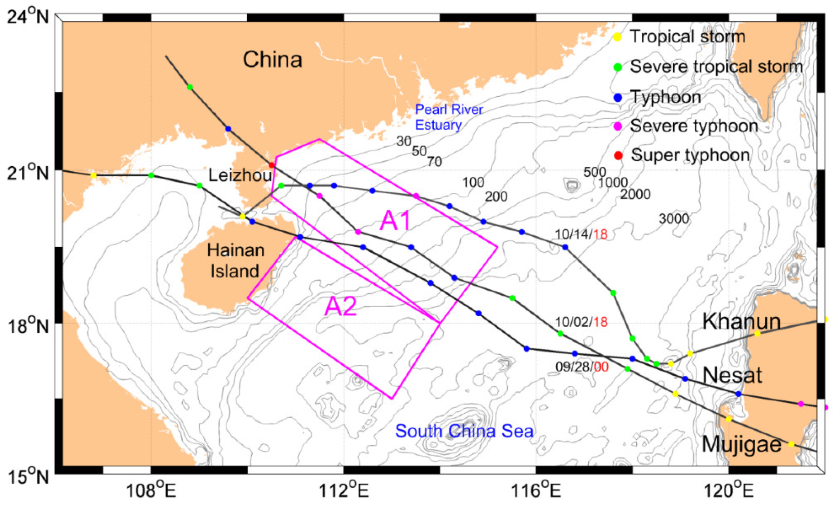
2.1. Study Area
2.2. Late Autumn Typhoons
2.3. Satellite Ocean Color Data
2.4. TSS Retrieval
2.5. CDOM Retrieval
2.6. Sea Level Anomaly and Geostrophic Current
2.7. Sea Surface Wind and Ekman Pumping
3. Climatological and Time Series Analyses
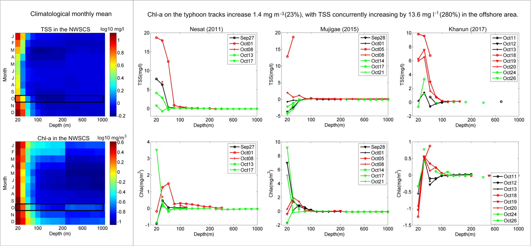
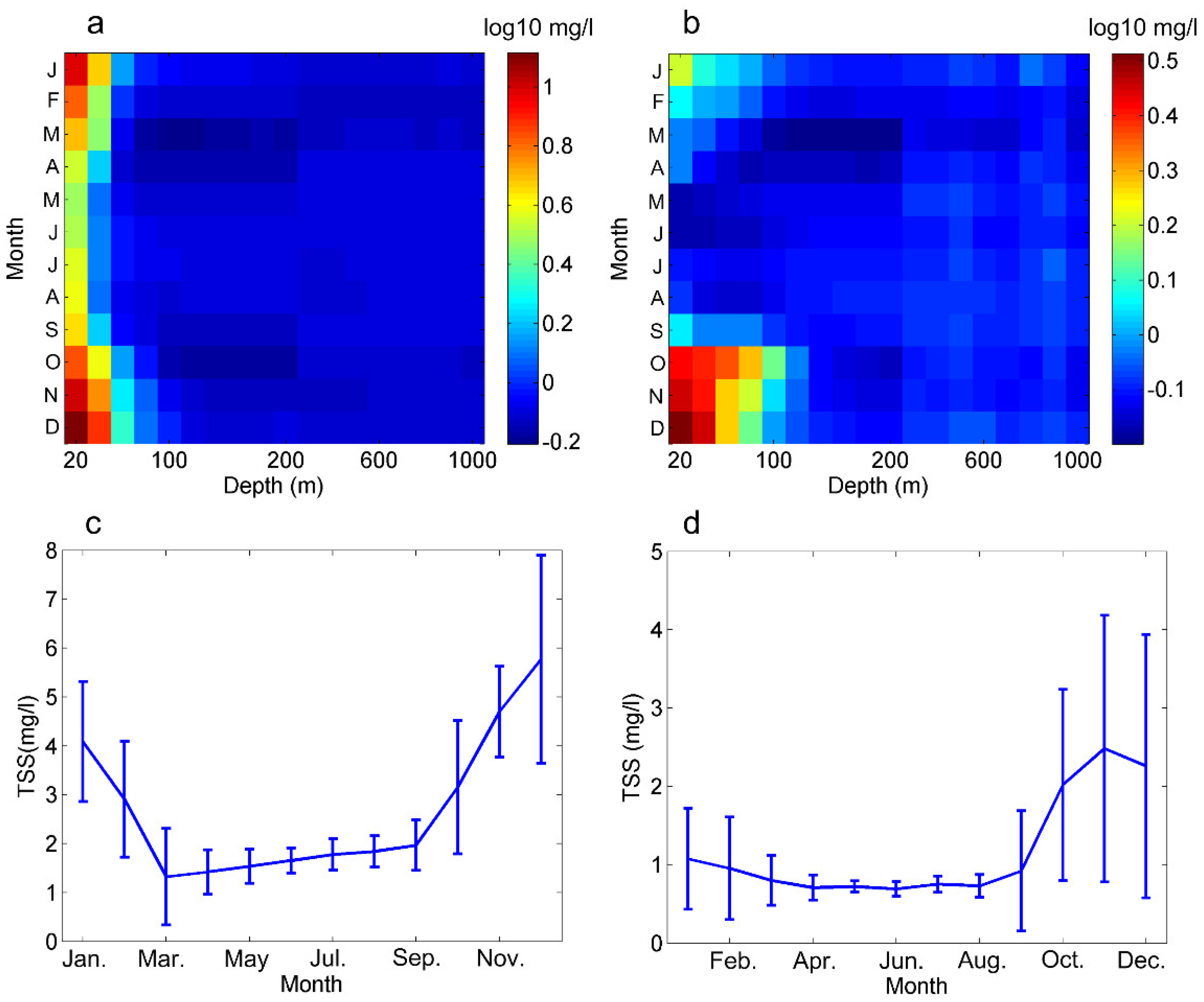
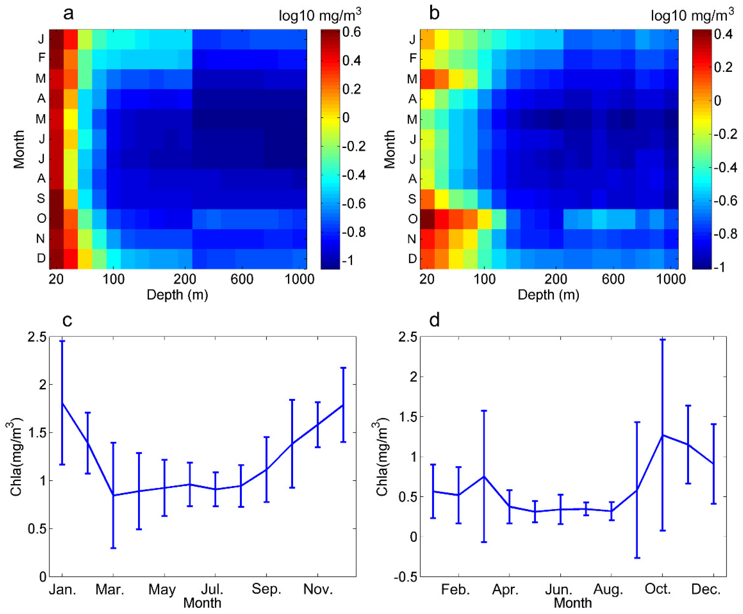
3.1. Monthly Variations of TSS and Chl-a Concentrations
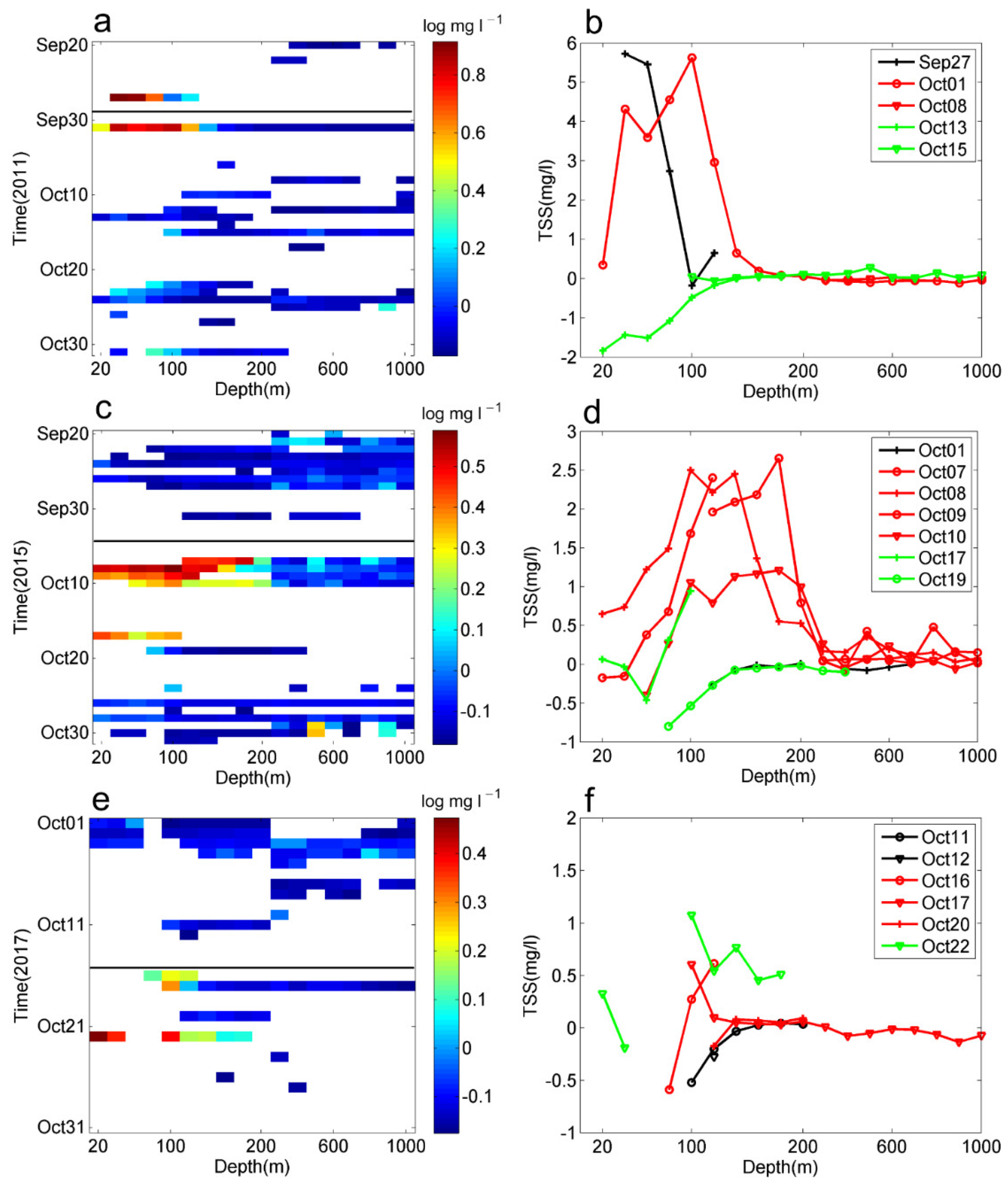
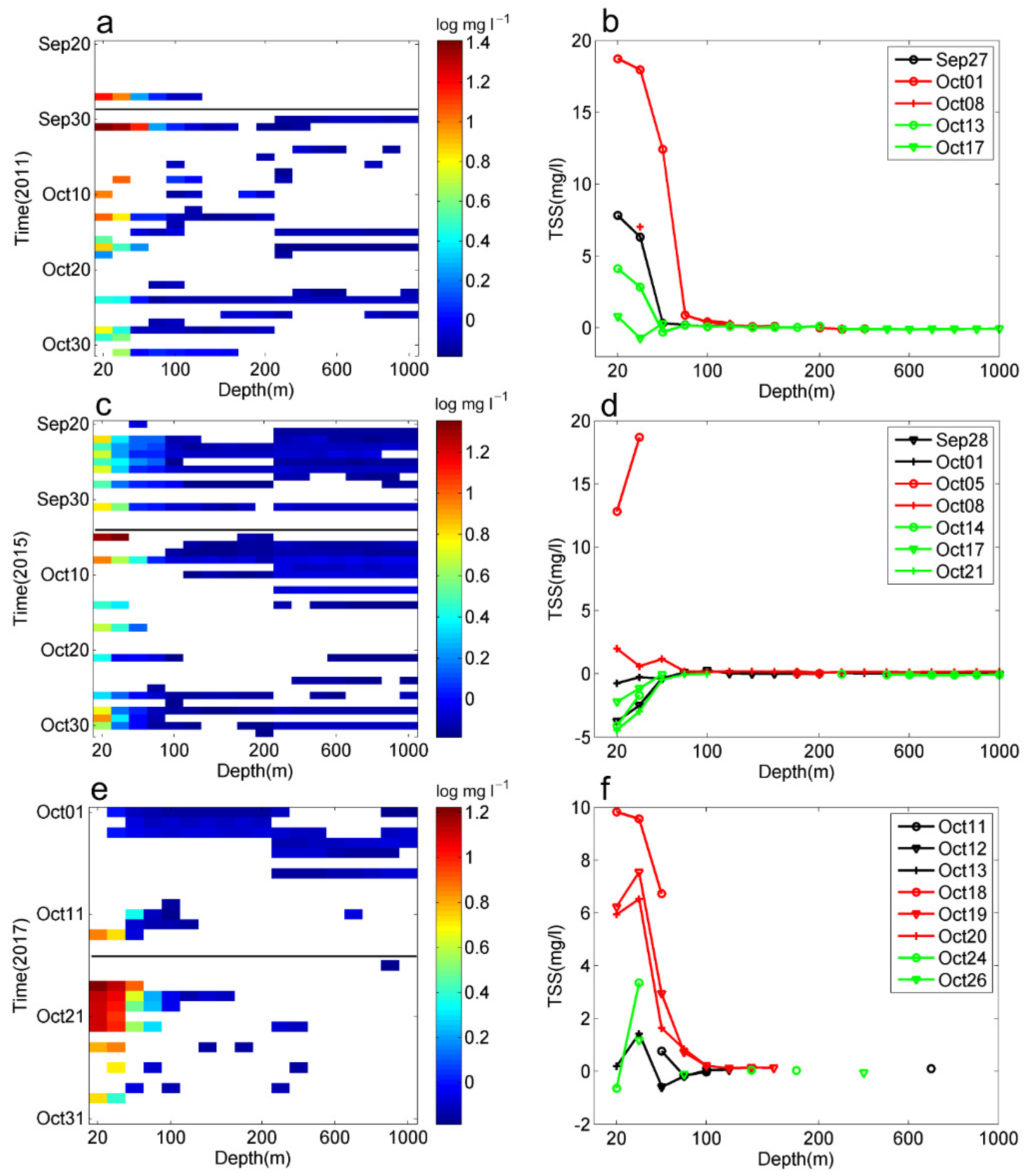
3.2. TSS and Chl-a Concentrations in A1 during the Typhoon Period
3.3. TSS and Chl-a Concentrations in A2 during the Typhoon Period
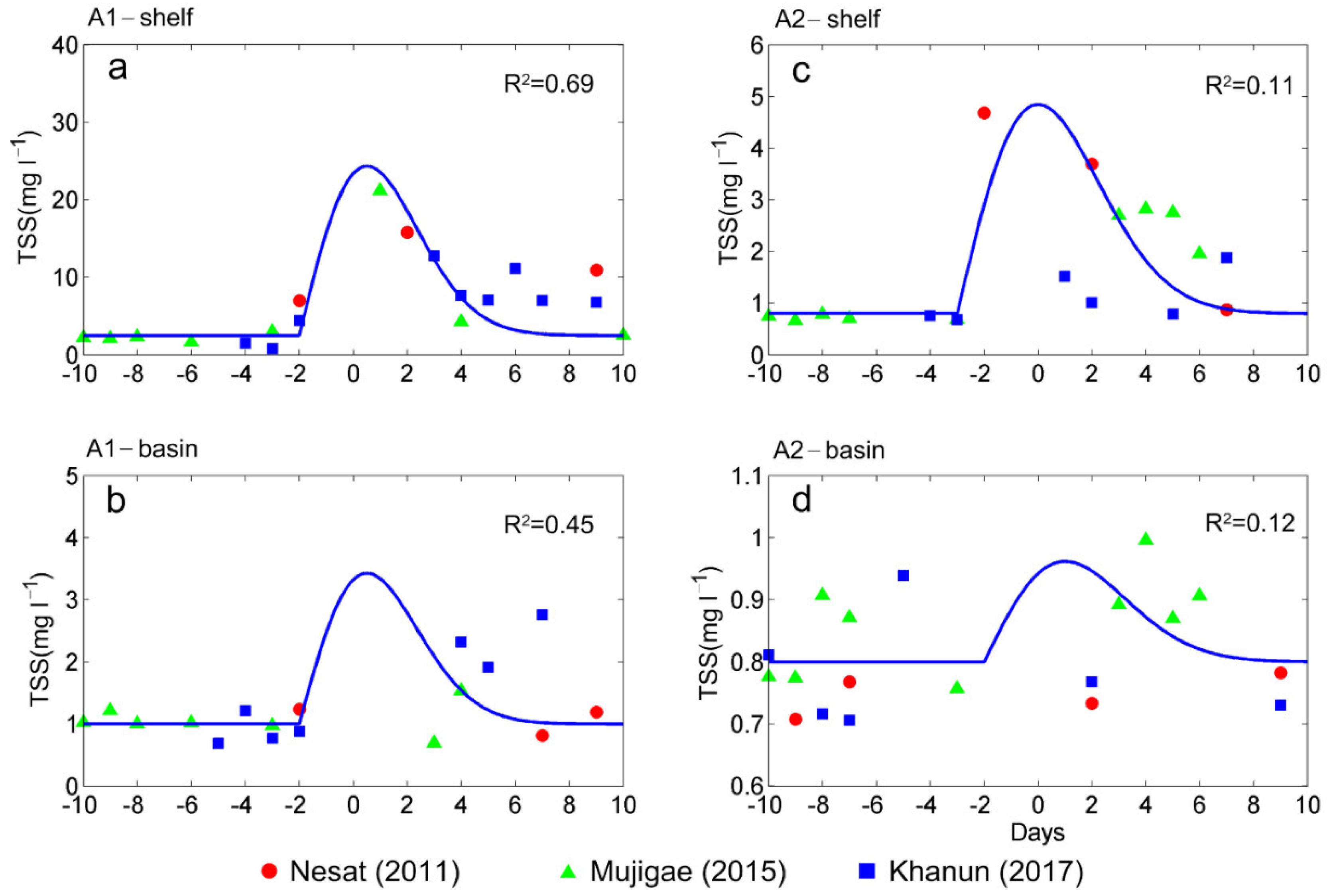
4. Empirical Analysis of Temporal Variations
5. Discussion
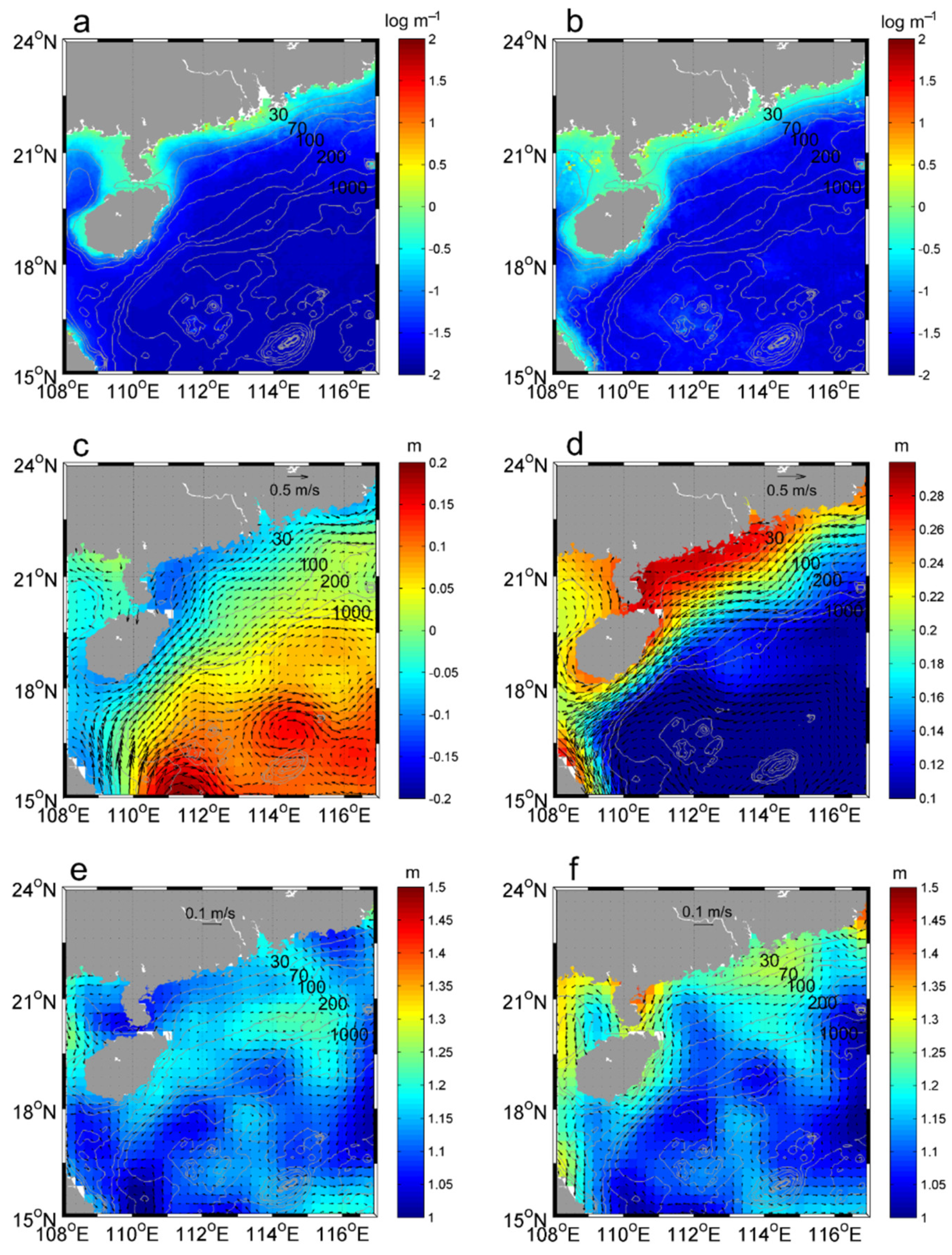
5.1. Pearl River Water Transport
5.2. Upwelling Effect and Mixing
6. Conclusions
Author Contributions
Funding
Institutional Review Board Statement
Informed Consent Statement
Data Availability Statement
Acknowledgments
Conflicts of Interest
References
- Hu, J.; Kawmura, H. Detection of cyclonic eddy generated by looping tropical cyclone in the northern South China Sea: A case study. Acta Oceanol. Sin. 2004, 232, 213–224. [Google Scholar]
- Zheng, Q.; Xie, L.; Xiong, X.; Hu, X.; Chen, L. Progress in research of submesoscale processes in the South China Sea. Acta Oceanol. Sin. 2020, 39, 1–13. [Google Scholar] [CrossRef]
- Guan, S.; Wei, Z.; Huthnance, J.; Tian, J.; Wang, J. Observed upper ocean response to typhoon Megi (2010) in the Northern South China Sea. J. Geophys. Res. Oceans 2014, 119, 3134–3157. [Google Scholar] [CrossRef] [Green Version]
- Sun, Z.; Hu, J.; Zheng, Q.; Gan, J. Comparison of typhoon-induced near-inertial oscillations in shear flow in the northern South China Sea. Acta Oceanol. Sin. 2015, 45, 38–45. [Google Scholar] [CrossRef]
- Lu, Z.; Wang, G.; Shang, X. Strength and Spatial Structure of the Perturbation Induced by a Tropical Cyclone to the Underlying Eddies. J. Geophys. Res. Oceans 2020, 125, e2020JC016097. [Google Scholar] [CrossRef]
- Sun, J.; Wang, G.; Xiong, X.; Hui, Z.; Hu, X.; Ling, Z.; Long, Y.; Yang, G.; Guo, Y.; Ju, X.; et al. Impact of warm mesoscale eddy on tropical cyclone intensity. Acta Oceanol. Sin. 2020, 39, 1–13. [Google Scholar] [CrossRef]
- Shang, S.; Li, L.; Sun, F.; Wu, J.; Hu, C.; Chen, D.; Ning, X.; Qiu, Y.; Zhang, C.; Shang, S. Changes of temperature and bio-optical properties in the South China Sea in response to Typhoon Lingling, 2001. Geophys. Res. Lett. 2008, 35, L10602. [Google Scholar] [CrossRef] [Green Version]
- Zhao, H.; Pan, J.; Han, G.; Devlin, A.T.; Zhang, S.; Hou, Y. Effect of a fast-moving tropical storm Washi on phytoplankton in the northwestern South China Sea. J. Geophys. Res. Oceans 2017, 122, 3404–3416. [Google Scholar] [CrossRef]
- Zhang, S.; Xie, L.; Hou, Y.; Zhao, H.; Qi, Y.; Yi, X. Tropical storm-induced turbulent mixing and chlorophyll-a enhancement in the continental shelf southeast of Hainan Island. J. Mar. Syst. 2014, 129, 405–414. [Google Scholar] [CrossRef] [Green Version]
- Liu, Y.; Tang, D.; Morozov, E. Chlorophyll Concentration Response to the Typhoon Wind-Pump Induced Upper Ocean Processes Considering Air–Sea Heat Exchange. Remote Sens. 2019, 11, 1825. [Google Scholar] [CrossRef] [Green Version]
- Yasuki, N.; Suzki, K.; Tsuda, A. Responses of lower trophic-level organisms to typhoon passage on the outer shelf of the East China Sea: An incubation experiment. Biogeosic. Discuss. 2013, 10, 6605–6635. [Google Scholar]
- Li, J.; Zheng, Q.; Li, M.; Li, Q.; Xie, L. Spatiotemporal Distributions of Ocean Color Elements in Response to Tropical Cyclone: A Case Study of Typhoon Mangkhut (2018) Past over the Northern South China Sea. Remote Sens. 2021, 13, 687. [Google Scholar] [CrossRef]
- Wang, Y. Composite of Typhoon-Induced Sea Surface Temperature and Chlorophyll-a Responses in the South China Sea. J. Geophys. Res. Oceans 2020, 125, e2020JC016243. [Google Scholar] [CrossRef]
- Wang, G.; Su, J.; Ding, Y.; Chen, D. Tropical cyclone genesis over the south China sea. J. Mar. Syst. 2007, 68, 318–326. [Google Scholar] [CrossRef]
- Huynh, H.; Alvera-Azcarate, A.; Beckers, J.M. Analysis of surface chlorophyll a associated with sea surface temperature and surface wind in the South China Sea. Ocean Dyn. 2020, 70, 139–161. [Google Scholar] [CrossRef]
- Wang, T.; Zhang, S.; Chen, F.; Ma, Y.; Jiang, C.; Yu, J. Influence of sequential tropical cyclones on phytoplankton blooms in the northwestern South China Sea. Chin. J. Oceanol. Limnol. 2020. [Google Scholar] [CrossRef]
- Shi, Y.; Xie, l.; Wang, L.; Zheng, M.; Shen, Y. Impacts of Typhoon Mujigea on Sea Surface Temperature and Chlorophyll-a Concentration in the Coastal Ocean of Western Guangdong. J. Guangdong Ocean Univ. 2017, 37, 49–58. (In Chinese) [Google Scholar]
- Shi, Y.; Xie, L.; Zheng, Q.; Zhang, S.; Li, J. Unusual coastal ocean cooling in the northern South China Sea by a katabatic cold jet associated with Typhoon Mujigea. Acta Oceanol. Sin. 2019, 38, 62–75. [Google Scholar] [CrossRef]
- Ding, Y.; Yao, Z.; Zhou, L.; Bao, M.; Zang, Z. Numerical modeling of the seasonal circulation in the coastal ocean of the Northern South China Sea. Front. Earth Sci. 2018, 14, 90–109. [Google Scholar] [CrossRef]
- Xie, L.L.; Cao, R.X.; Shang, Q.T. Progress of Study on Coastal Circulation near the Shore of Western Guangdong. J. Guangdong Ocean Univ. 2012, 32, 94–98. (In Chinese) [Google Scholar]
- Ding, Y.; Bao, X.; Yao, Z.; Zhang, C.; Wan, K.; Bao, M.; Li, R.; Shi, M. A modeling study of the characteristics and mechanism of the westward coastal current during summer in the northwestern South China Sea. Ocean Sci. J. 2017, 52, 11–30. [Google Scholar] [CrossRef]
- Li, R.; Chen, C.; Xia, H.; Beardsley, R.C.; Shi, M.; Lai, Z.; Lin, H.; Feng, Y.; Liu, C.; Xu, Q.; et al. Observed wintertime tidal and subtidal currents over the continental shelf in the northern South China Sea. J. Geophys. Res. Oceans 2014, 119, 5289–5310. [Google Scholar] [CrossRef]
- Zheng, M.; Li, M.; Xie, L.; Hong, Y.; He, Y.; Zong, X. Observation of hydrographic characteristics of northwestern shelf of the South China Sea in winter 2012. Oceanol. Et Limnol. Sin. 2018, 49, 734–745. (In Chinese) [Google Scholar] [CrossRef]
- Shan, G.; Hui, W.; Gui-Mei, L.; Liang-Min, H. The statistical estimation of the vertical distribution of chlorophyll a concentration in the South China Sea. Acta Oceanol. Sin. 2010, 5, 13–26. [Google Scholar]
- Liao, X.; Dai, M.; Gong, X.; Liu, H.; Huang, H. Subsurface chlorophyll a maximum and its possible causes in the southern South China Sea. J. Trop. Oceanogr. 2018, 37, 45–56. [Google Scholar] [CrossRef]
- Ravichandran, M.; Girishkumar, M.S.; Riser, S. Observed variability of chrolophyll-a using Argo profiling floats in the southeastern Arabian Sea. Deep Sea Res. Part I Oceanogr. Res. Pap. 2012, 65, 15–25. [Google Scholar] [CrossRef]
- Xie, L.L.; Zhang, S.W. Overview of studies on Qiongdong upwelling. J. Trop. Oceanogr. 2012, 31, 35–41. (In Chinese) [Google Scholar]
- Lü, H.; Ma, X.; Wang, Y.; Xue, H.; Chai, F. Impacts of the unique landfall Typhoons Damrey on chlorophyll-a in the Yellow Sea off Jiangsu Province, China. Reg. Stud. Mar. Sci. 2020, 39, 101394. [Google Scholar] [CrossRef]
- Zheng, Q.; And, G.F.; Song, Y.T. Introduction to special section: Dynamics and Circulation of the Yellow, East, and South China Seas. J. Geophys. Res. Oceans 2006, 111, C11. [Google Scholar] [CrossRef] [Green Version]
- Hu, J.; Kawamura, H.; Li, C.; Hong, H.; Jiang, Y. Review on Current and Seawater Volume Transport through the Taiwan Strait. J. Oceanogr. 2010, 66, 591–610. [Google Scholar] [CrossRef] [Green Version]
- Hu, J.; Wang, X.H. Progress on upwelling studies in the China seas. Rev. Geophys. 2016, 54, 653–673. [Google Scholar] [CrossRef]
- Shi, W.; Huang, Z.; Hu, J. Using TPI to Map Spatial and Temporal Variations of Significant Coastal Upwelling in the Northern South China Sea. Remote Sens. 2021, 13, 1065. [Google Scholar] [CrossRef]
- Xie, L.; Pallas-Sanz, E.; Zheng, Q.; Zhang, S.; Zong, X.; Yi, X.; Li, M. Diagnosis of 3-D vertical circulation in the upwelling and frontal zones east of Hainan Island, China. J. Phys. Oceanogr. 2017, 47, 755–774. [Google Scholar] [CrossRef]
- Lu, X.; Yu, H.; Ying, M.; Zhao, B.; Zhang, S.; Lin, L.; Bai, L.; Wan, R. Western North Pacific Tropical Cyclone Database Created by the China Meteorological Administration. Adv. Atmos. Sci. 2021, 38, 690–699. [Google Scholar] [CrossRef]
- Ying, M.; Zhang, W.; Yu, H.; Lu, X.; Feng, J.; Fan, Y.; Zhu, Y.; Chen, D. An Overview of the China Meteorological Administration Tropical Cyclone Database. J. Atmos. Ocean. Technol. 2014, 31, 287–301. [Google Scholar] [CrossRef] [Green Version]
- Kahru, M.; Kudela, R.M.; Lorenzo, E.; Manzano-Saraba, M.; Mitchell, B.G. Trends in the surface chlorophyll of the California Current: Merging data from multiple ocean color satellites. Deep Sea Res. Part II Top. Stud. Oceanogr. 2012, 77–80, 89–98. [Google Scholar] [CrossRef]
- Teodoro, A.C.; Veloso-Gomes, F. Quantification of the Total Suspended Matter concentration around the sea breaking zone from in situ measurements and TERRA/ASTER data. Mar. Georesour. Geotechnol. 2007, 25, 67–80. [Google Scholar] [CrossRef]
- Teodoro, A.C.; Veloso-Gomes, F.; Goncalves, H. Retrieving TSM Concentration from Multispectral Satellite Data by Multiple Regression and Artificial Neural Networks. IEEE Trans. Geosci. Remote Sens. 2007, 45, 1342–1350. [Google Scholar] [CrossRef]
- Miller, R.; McKee, B. Using MODIS Terra 250 m imagery to map concentrations of total suspended matter in coastal waters. Remote Sens. Environ. 2004, 93, 259–266. [Google Scholar] [CrossRef]
- Tassan, S. An Improved In-Water Algorithm for the Determination of Chlorophyll and Suspended Sediment Concentration from Thematic Mapper Data in Coastal Waters. Int. J. Remote Sens. 1993, 14, 1221–1229. [Google Scholar] [CrossRef]
- Zhang, M.; Tang, J.; Dong, Q.; Song, Q.; Ding, J. Retrieval of total suspended matter concentration in the Yellow and East China Seas from MODIS imagery. Remote Sens. Environ. 2010, 114, 392–403. [Google Scholar] [CrossRef]
- Asaoka, S.; Nakada, S.; Umehara, A.; Ishizaka, J.; Nishijima, W. Estimation of spatial distribution of coastal ocean primary production in Hiroshima Bay, Japan, with a geostationary ocean color satellite. Estuar. Coast. Shelf Sci. 2020, 244, 106897. [Google Scholar] [CrossRef]
- Nakada, S.; Kobayashi, S.; Hayashi, M.; Ishizaka, J.; Akiyama, S.; Fuchi, M.; Nakajima, M. High-resolution surface salinity maps in coastal oceans based on geostationary ocean color images: Quantitative analysis of river plume dynamics. J. Oceanogr. 2018, 74, 287–304. [Google Scholar] [CrossRef]
- Enriquez, A.; Friehe, C. Effects of Wind Stress and Wind Stress Curl Variability on Coastal Upwelling. J. Phys. Oceanogr. 1995, 25, 1651–1671. [Google Scholar] [CrossRef] [Green Version]
- Chen, X.; Pan, D.; He, X.; Bai, Y.; Wang, D. Upper ocean responses to category 5 typhoon Megi in the western north Pacific. Acta Oceanol. Sin. 2012, 1, 51–58. [Google Scholar] [CrossRef]
- Hellerman, S.; Rosenstein, M. Normal Monthly Wind Stress over the World Ocean with Error Estimates. J. Phys. Oceanogr. 1983, 13, 1093–1104. [Google Scholar] [CrossRef] [Green Version]
- Garratt, J.R. Review of Drag Coefficients over Oceans and Continents. Mon. Weather Rev. 1977, 105, 915–929. [Google Scholar] [CrossRef] [Green Version]
- Pan, G.; Chai, F.; Tang, D.; Wang, D. Marine phytoplankton biomass responses to typhoon events in the South China Sea based on physical-biogeochemical model. Ecol. Model. 2017, 356, 38–47. [Google Scholar] [CrossRef]
- Zheng, G.; Tang, D. Offshore and nearshore chlorophyll increases induced by typhoon winds and subsequent terrestrial rainwater runoff. Mar. Ecol. Prog. Ser. 2007, 333, 61–74. [Google Scholar] [CrossRef] [Green Version]
- Ye, H.J.; Sui, Y.; Tang, D.L.; Afanasyev, Y.D. A subsurface chlorophyll a bloom induced by typhoon in the South China Sea. J. Mar. Syst. 2013, 128, 138–145. [Google Scholar] [CrossRef]
- Zhao, H.; Tang, D.; Wang, D. Phytoplankton blooms near the Pearl River Estuary induced by Typhoon Nuri. J. Geophys. Res. 2009, 114, C12027. [Google Scholar] [CrossRef]
- Wang, Z.; Li, W.; Zhang, K.; Agrawal, Y.C.; Huang, H. Observations of the distribution and flocculation of suspended particulate matter in the North Yellow Sea cold water mass. Cont. Shelf Res. 2020, 204, 104187. [Google Scholar] [CrossRef]
- Chen, Y.Q.; Tang, D.L. Remote Sensing Analysis of Impact of Typhoon on Environment in the Sea Area South of Hainan Island. Procedia Environ. Sci. 2011, 10, 1621–1629. [Google Scholar]
- Yu, X.; Xu, J.; Long, A.; Li, R.; Shi, Z.; Li, Q.P. Carbon-to-chlorophyll ratio and carbon content of phytoplankton community at the surface in coastal waters adjacent to the Zhujiang River Estuary during summer. Acta Oceanol. Sin. 2020, 39, 123–131. [Google Scholar] [CrossRef]
- Hu, B.; Wang, P.; Bao, T.; Qian, J.; Wang, X. Mechanisms of photochemical release of dissolved organic matter and iron from resuspended sediments. J. Environ. Sci. 2021, 104, 288–295. [Google Scholar] [CrossRef] [PubMed]
- Southwell, M.W.; Kieber, R.J.; Mead, R.N.; Avery, G.B.; Skrabal, S.A. Effects of sunlight on the production of dissolved organic and inorganic nutrients from resuspended sediments. Biogeochemistry 2010, 98, 115–126. [Google Scholar] [CrossRef]
- Shank, G.C.; Evans, A.; Jaffé, R.; Yamashita, Y. Influence of solar radiation on DOM release from resuspended Florida Bay sediments. In Proceedings of the AGU Fall Meeting Abstracts, San Francisco, CA, USA, 14–18 December 2019. [Google Scholar]
- Schiebel, H.N.; Wang, X.; Chen, R.F.; Peri, F. Photochemical Release of Dissolved Organic Matter from Resuspended Salt Marsh Sediments. Estuaries Coasts 2015, 38, 1692–1705. [Google Scholar] [CrossRef]
- Bai, Y.; Su, R.; Han, X.; Zhang, C.; Shi, X. Investigation of seasonal variability of CDOM fluorescence in the southern Changjiang River Estuary by EEM-PARAFAC. Acta Oceanol. Sin. 2015, 34, 1–12. [Google Scholar] [CrossRef]
- Huang, C.; Chen, F.; Zhang, S.; Chen, C.; Meng, Y.; Zhu, Q.; Song, Z. Carbon and nitrogen isotopic composition of particulate organic matter in the Pearl River Estuary and the adjacent shelf. Estuar. Coast. Shelf Sci. 2020, 246, 107003. [Google Scholar] [CrossRef]
- Lao, Q.; Chen, F.; Liu, G.; Chen, C.; Jin, G.; Zhu, Q.; Wei, C.; Zhang, C. Isotopic evidence for the shift of nitrate sources and active biological transformation on the western coast of Guangdong Province, South China. Mar. Pollut. Bull. 2019, 142, 603–612. [Google Scholar] [CrossRef]
- Yang, Y.; Yan-Dong, X.U.; Wang, F.Y.; Wei, X. A Numerical Hydrodynamic and Transport Model in the West Coast of Guangdong Province. Sci. Technol. Eng. 2015, 19, 86–91. [Google Scholar]
- Huang, Y.; Chen, F.; Zhao, H.; Zeng, Z.; Chen, J. Concentration distribution and structural features of nutrients in the northwest of the South China Sea in winter 2012. J. Appl. Oceanogr. 2015, 34, 310–316. (In Chinese) [Google Scholar]
- Zheng, M.; Xie, L.; Zheng, Q.; Li, M.; Li, J. Volume and Nutrient Transports Disturbed by the Typhoon Chebi (2013) in the Upwelling Zone East of Hainan Island, China. J. Mar. Sci. Eng. 2021, 9, 324. [Google Scholar] [CrossRef]
- Wang, L.; Xie, L.; Zheng, Q.; Li, J.; Li, M.; Hou, Y. Tropical cyclone enhanced vertical transport in the northwestern South China Sea I: Mooring observation analysis for Washi (2005). Estuar. Coast. Shelf Sci. 2020, 235, 106599. [Google Scholar] [CrossRef]
- Jiang, C.; Cao, R.; Lao, Q.; Chen, F.; Zhang, S.; Bian, P. Typhoon Merbok induced upwelling impact on material transport in the coastal northern South China Sea. PLoS ONE 2020, 15, e0228220. [Google Scholar] [CrossRef]
- Wong, G.; Pan, X.; Li, K.-Y.; Shiah, F.-K.; Ho, T.-Y.; Guo, X. Hydrography and nutrient Dynamics in the Northern South China Sea Shelf-sea (NoSoCS). Deep Sea Res. Part II Top. Stud. Oceanogr. 2015, 117, 23–40. [Google Scholar] [CrossRef]


| Typhoon | Date | Category | Origin |
|---|---|---|---|
| Nesat | 24–30 September 2011 | Typhoon | Pacific Ocean |
| Mujigae | 02–05 October 2015 | Super typhoon | Pacific Ocean |
| Khanun | 11–16 October 2017 | Typhoon | Pacific Ocean |
| Time Period | Data | Temporal Resolution | Spatial Resolution | Satellite/Sensor |
|---|---|---|---|---|
| 19–31 September 2011 | Chl-a, Rrs645 | daily | 4 km | Terra, Aqua/MODIS |
| 20 September–31 October 2015 | Chl-a, Rrs645 | daily | 4 km | Terra, Aqua/MODIS |
| 01–31 October 2017 | Chl-a, Rrs645 | daily | 4 km | Terra, Aqua/MODIS |
| 2004–2019 | Chl-a, Rrs412, Rrs555, Rrs645 | monthly | 4 km | Terra Aqua/MODIS |
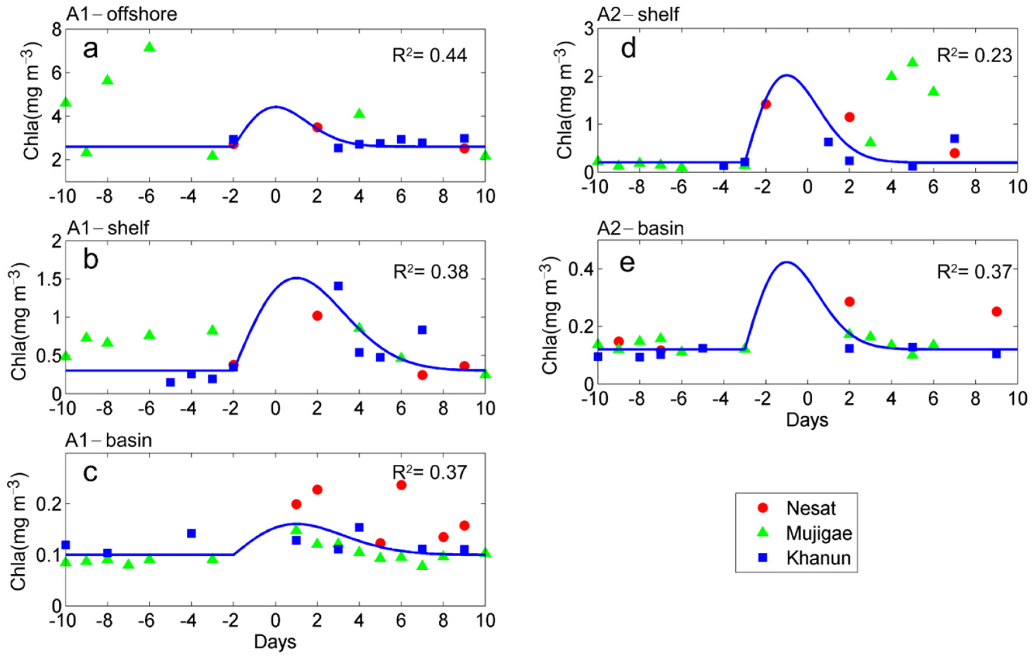
| Area | ∆TSS (mg L−1) | ATSS (mg L−1) | T (d) | σ2 | R2 | ∆Chl-a (mg m−3) | AChl-a (mg L−1) | T (d) | σ2 | R2 | |
|---|---|---|---|---|---|---|---|---|---|---|---|
| A1 | Offshore | 2.5 | 90 | 2 | 2.5 | 0.69 | 2.6 | 6 | 2 | 2 | 0.44 |
| Shelf | 0.3 | 6 | 2 | 3 | 0.39 | ||||||
| Basin | 1 | 10 | 2 | 2.5 | 0.45 | 0.1 | 0.3 | 2 | 3 | 0.37 | |
| A2 | Shelf | 0.8 | 20 | 3 | 3 | 0.11 | 0.2 | 6 | 3 | 2 | 0.23 |
| Basin | 0.8 | 0.8 | 3 | 3 | 0.12 | 0.12 | 1 | 3 | 2 | 0.37 | |
Publisher’s Note: MDPI stays neutral with regard to jurisdictional claims in published maps and institutional affiliations. |
© 2021 by the authors. Licensee MDPI, Basel, Switzerland. This article is an open access article distributed under the terms and conditions of the Creative Commons Attribution (CC BY) license (https://creativecommons.org/licenses/by/4.0/).
Share and Cite
Li, J.; Zheng, H.; Xie, L.; Zheng, Q.; Ling, Z.; Li, M. Response of Total Suspended Sediment and Chlorophyll-a Concentration to Late Autumn Typhoon Events in the Northwestern South China Sea. Remote Sens. 2021, 13, 2863. https://0-doi-org.brum.beds.ac.uk/10.3390/rs13152863
Li J, Zheng H, Xie L, Zheng Q, Ling Z, Li M. Response of Total Suspended Sediment and Chlorophyll-a Concentration to Late Autumn Typhoon Events in the Northwestern South China Sea. Remote Sensing. 2021; 13(15):2863. https://0-doi-org.brum.beds.ac.uk/10.3390/rs13152863
Chicago/Turabian StyleLi, Junyi, Huiyuan Zheng, Lingling Xie, Quanan Zheng, Zheng Ling, and Min Li. 2021. "Response of Total Suspended Sediment and Chlorophyll-a Concentration to Late Autumn Typhoon Events in the Northwestern South China Sea" Remote Sensing 13, no. 15: 2863. https://0-doi-org.brum.beds.ac.uk/10.3390/rs13152863