
Application of SAR Data for Tropical Cyclone Intensity Parameters Retrieval and Symmetric Wind Field Model Development


1
College of Oceanography and Space Informatics, China University of Petroleum, Qingdao 266580, China
2
Physical Oceanography Laboratory, Ocean University of China, Qingdao 266100, China
*
Author to whom correspondence should be addressed.
Remote Sens. 2021, 13(15), 2902; https://0-doi-org.brum.beds.ac.uk/10.3390/rs13152902
Submission received: 17 June 2021
/
Revised: 17 July 2021
/
Accepted: 20 July 2021
/
Published: 23 July 2021
(This article belongs to the Special Issue Added-Value SAR Products for the Observation of Coastal Areas)
Abstract
:The spaceborne synthetic aperture radar (SAR) is an effective tool to observe tropical cyclone (TC) wind fields at very high spatial resolutions. TC wind speeds can be retrieved from cross-polarization signals without wind direction inputs. This paper proposed methodologies to retrieve TC intensity parameters; for example, surface maximum wind speed, TC fullness (TCF) and central surface pressure from the European Space Agency Sentinel-1 Extra Wide swath mode cross-polarization data. First, the MS1A geophysical model function was modified from 6 to 69 m/s, based on three TC samples’ SAR images and the collocated National Oceanic and Atmospheric Administration stepped frequency microwave radiometer wind speed measurements. Second, we retrieved the wind fields and maximum wind speeds of 42 TC samples up to category 5 acquired in the last five years, using the modified MS1A model. Third, the TCF values and central surface pressures were calculated from the 1-km wind retrievals, according to the radial curve fitting of wind speeds and two hurricane wind-pressure models. Three intensity parameters were found to be dependent upon each other. Compared with the best-track data, the averaged bias, correlation coefficient (Cor) and root mean-square error (RMSE) of the SAR-retrieved maximum wind speeds were –3.91 m/s, 0.88 and 7.99 m/s respectively, showing a better result than the retrievals before modification. For central pressure, the averaged bias, Cor and RMSE were 1.17 mb, 0.77 and 21.29 mb and respectively, indicating the accuracy of the proposed methodology for pressure retrieval. Finally, a new symmetric TC wind field model was developed with the fitting function of the TCF values and maximum wind speeds, radial wind curve and the Rankine Vortex model. By this model, TC wind field can be simulated just using the maximum wind speed and the radius of maximum wind speed. Compared with wind retrievals, averaged absolute bias and averaged RMSE of all samples’ wind fields simulated by the new model were smaller than those of the Rankine Vortex model.
1. Introduction
Tropical cyclones (TCs) are one of the most destructive natural disasters on earth, including typhoons in western Pacific Ocean and hurricanes in Atlantic Ocean, Caribbean Ocean, and eastern Pacific Ocean. It forms over warm tropical waters with air accelerating towards a central low pressure [1]. TC intensity is defined in terms of the associated destruction when the storm arrives on land and is generally measured by serval parameters, for example, surface (10-m height) maximum wind speed, central surface pressure and TC fullness (TCF) [2,3].
In meteorology, surface maximum wind speed is defined as the time-averaged maximum wind in the TC eyewall region. Both Saffir-Simpson hurricane intensity categories and the east Asian intensity definition are based on surface maximum wind speed, despite different averaged durations [4]. A strong storm tends to have a lower central pressure. The difference between central surface pressure and ambient surface pressure is the dominant factor for generating gradient wind and has a positive correlation with maximum wind speed [5]. Wind-pressure models relate wind speed to pressure, which are widely utilized to estimate or simulate the wind field from limited pressure observations and vice versa [6,7,8].
In order to measure the size of the TC wind field, the radius of the maximum wind (RMW) and the radius of the gale-force wind (R17) are defined as size parameters. They receive particular attention and are used by former analysis to document the structure and the strength evolution of TC systems [9,10,11]. RMW describes the radius of extreme wind near the eyewall and R17 describes the extent of TC outer circulation. TCF bridges the gap between size and intensity, whose variation indicates TC’s intensification [12]. In general, a TC is considered to be intense when it has a small RMW and a large R17, corresponding to a large TCF value, and weak when it has a large RMW and a small R17, corresponding to a small TCF value [3].
Spaceborne active microwave radars, such as scatterometers and synthetic aperture radars (SAR), can be employed day and night for monitoring TC systems over oceans [13,14]. Based on the positive correlation between microwave backscattering and sea surface roughness, sea surface wind speed can be retrieved by geophysical model functions (GMF) from different polarization channels [15,16,17]. The GMF usually refers to the empirical formula relating a normalized radar cross section (NRCS) to wind vector and radar incident angles. Due to the limitation of Bragg scattering, the co-polarization (VV or HH) NRCS becomes saturated with wind increasing under TC conditions. For example, the VV-polarization NRCS does not increase when the wind speed exceeds 25 m/s, leading to the retrieval problem of hurricane wind speeds, because the lower limit of the category 1 hurricane is 33 m/s [18].
With improvement of the active microwave radar technology, cross-polarization (VH or HV) NRCS is found to be unsaturated, even under extreme wind conditions, because the cross-polarization echo signals are sensitive to wave breaking [19,20]. Hence, SAR cross-polarization signals are more suitable for retrieving TC surface wind speeds, which provides a valuable data source with high spatial resolution for studying detailed storm field structures [21,22]. It has been indicated that the cross-polarization NRCS is dependent upon wind speed and radar incident angle, and is independent of wind direction [23,24]. For extreme wind speed, the incidence angle dependency is found to be weak [16]. The cross-polarization GMF based on this relationship is the foundation of retrieving TC wind speeds from SAR images, which influences the accuracy of TC intensity parameter retrieval directly. According to the collocations of SAR data and a variety of wind speed measurements or simulations, a large number of cross-polarization GMFs have been established empirically, such as the H14 model [25] and the MS1A model [26].
Based on the Radarsat-2 dual-polarization ScanSAR mode products, Hwang et al. proposed the H14 GMF, which includes two models, i.e., H14S and H14E. The two models were established with the same design methodology, but from different wind references, leading to obviously different parameters. The wind sources of the former model were buoy, stepped frequency microwave radiometer (SFMR) and H*Wind data, whose maximum value was 56.00 m/s. For wind speeds higher than 35 m/s, VH NRCS acquired at incident angles lower than 45° was predicted to be saturated by the H14S model. The latter model was applicable to the European Center for Medium-range Weather Forecast (ECMWF) wind simulations, whose maximum value was 37.63 m/s. It has no saturation error for winds higher than 35 m/s. Validations suggested that the root mean squares (RMS) difference and bias were 2.45 and −0.32 m/s respectively for the H14E model.
By the same design methodology as the H14 model, the MS1A model was proposed based on the Sentinel-1A products acquired in Extra Wide swath (EW) mode and the soil moisture active passive (SMAP) wind speed measurements, whose maximum value is about 45 m/s. In their study, due to the limitation of SMAP data’s spatial resolution, VH NRCS values were averaged from a high spatial resolution (about 90 m) to a coarser spatial resolution (40 km). The 3-km retrievals were not validated. This shortcoming was mainly caused by the problem of wind reference availability in the Satellite Hurricane Observation Campaign (SHOC) during the 2016 hurricane season. There was only the Tropical Strom Karl collocated with SFMR measurements, meaning that the maximum wind speed was less than 33 m/s for this case. Although it has been indicated that the agreement between SMAP and SFMR for winds greater than 25 m/s is very good [27], the MS1A model still needs to be evaluated by comparing retrievals with SFMR data.
Using 3-km winds retrieved by the MS1AHW model, Combot et al. constructed an extensive database from RadarSat-2 and Sentinel-1 SAR acquisitions to describe how the SAR-derived wind field can be used to extract important TC parameters and evaluate their consistency with respect to best-track and SFMR airborne measurements [28]. While retrievals have a strong correlation with the SFMR data provided by Center for Satellite Applications and Research (STAR) of the National Environmental Satellite, Data, and Information Service (NESDIS), they have lower statistical outcomes with the SFMR data from Hurricane Research Division (HRD) of the Atlantic Oceanographic and Meteorological Laboratory (AOML), that we will use here. For AOML/HRD, bias and RMSE are 1.49 and 4.32 m/s, respectively. For STAR/NESDIS, bias and RMSE are −0.24 and 3.86 m/s, respectively.
In this study, we focus on the application of SAR data for TC intensity parameter retrieval and symmetric wind field model development. Following the introduction, the data used are introduced in Section 2. In Section 3, the MS1A-retrieved wind speeds are compared against the SFMR data for modification. In Section 4, we retrieve 42 TC samples’ wind fields by the modified MS1A model and extract their intensity parameters. Then, these parameters are analyzed statistically and compared with the best-track data. A new TC wind field model is developed in Section 5. Discussions and conclusions are made in Section 6 and Section 7, respectively.
2. Data
2.1. Sentinel-1 EW Mode Data
For the European Space Agency (ESA) Sentinel-1 A/B satellites, TC images are generally acquired in the EW mode or the Interferometric Wide swath (IW) mode. The two modes include both VV-polarization and VH-polarization channels. The EW mode images have a wider swath (400 km) and more sub-swaths (5) than the IW mode images (250-km swath and 3 sub-swaths), and sacrifice high spatial resolution for large coverage.
In this study, the L1-detected medium-resolution (GRD-MD) dual-polarization products in EW mode were collected from the ESA Copernicus Open Access Hub database (https://scihub.copernicus.eu/, accessed date: 21 April, 2021), including 68 scenes of 42 TC samples (23 hurricane samples and 19 typhoon samples) acquired in the past five years. Their brief information is listed in Appendix A Table A1 and Table A2. In the data processing step, the Sentinel Application Platform (SNAP) 7.0 software was utilized for GRD border noise removal, thermal noise removal, and image calibration. All images were resampled at a spatial resolution of 1 km, which is comparable to the SFMR data and is used throughout.
2.2. SFMR Wind Speed Measurements
As an airborne passive microwave radar, the National Oceanic and Atmospheric Administration (NOAA) SFMR is the primary instrument used by the National Hurricane Center (NHC) to determine hurricane intensity. SFMR measures surface brightness temperature along the flight track in 6 frequency bands spanning 4.6 to 7.2 GHz [29]. Wind speeds are retrieved based on the function between wind speed and brightness temperature. It was reported that the SFMR wind speed measurements were within ~3.9 m/s RMSE of the dropsonde-estimated wind speeds [30].
We collected the SFMR wind measurements of three TCs (Tropical Storm Karl, Hurricane Michael and Hurricane Douglas) from the NOAA Atlantic Oceanography and Meteorological Laboratory (AOML) (ftp://ftp.aoml.noaa.gov/hrd/pub/data/sfmr/, accessed date: 21 April 2021). The spatial resolution is 0.01°. The time difference between SFMR and SAR data were controlled within 2 h. The location shift algorithm proposed in [31] was applied for improving the collocation accuracy, which has been used previously in [16] and [32]. Due to Karl collocations’ small maximum wind (29.5 m/s) and small quantity in 20–30 m/s (only 73 points), we did not use it for GMF modification. Table 1 illustrates the TC information, SAR images and collocation numbers of the Hurricane Michael and the Hurricane Douglas.
2.3. TC Best-Track Data
The best-track data generally contain basic TC information, such as time, center location, maximum surface wind speed and central surface pressure. The best-tracks of 23 hurricane samples and 19 typhoon samples were collected from the NHC’s reports (https://www.nhc.noaa.gov/data/tcr/, accessed date: 24 April 2021) and the Joint Typhoon Warning Center (JTWC) (http://www.metoc.navy.mil/jtwc/, accessed date: 5 July 2021). Intensities provided by two centers are 1-min sustained winds. The data used were specified to be with the closest time to the SAR acquisition time. According to the best-tracks, Figure 1 shows the number of TC samples in different categories and different sea areas.
3. MS1A Modification
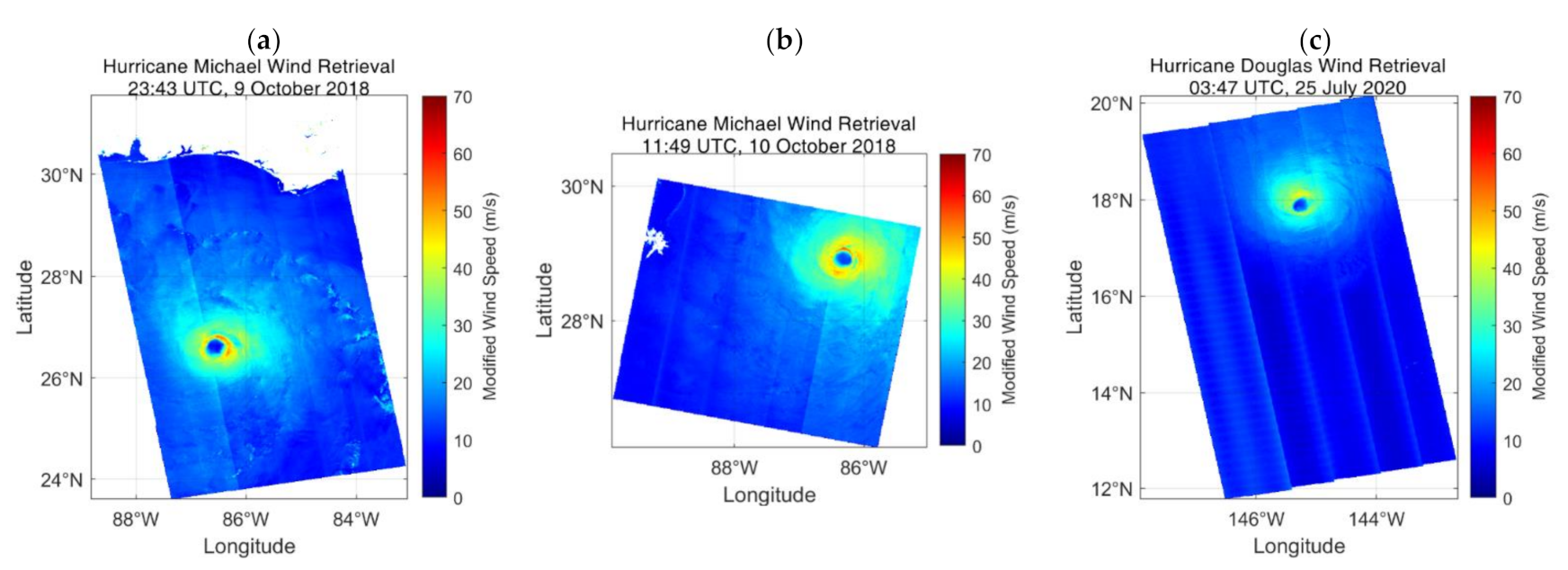
We retrieved the wind fields of the Hurricane Michael and the Hurricane Douglas from 3 Sentinel-1A VH-polarization images, based on the MS1A model proposed in [26]. The SAR images and retrievals are shown in Figure 2. Although there are some imprints of sub-swath seams in retrieval maps, the regions of wind speeds higher than 25 m/s are consecutive, indicating that the high wind speed region is free of thermal noise impact. For these samples, the SAR-retrieved maximum wind speeds are 72.05, 78.96 and 57.78 m/s in Figure 2d, e and f, respectively. However, according to the best-tracks, their maximum wind speeds were 110, 125 and 95 knots, i.e., 56.54, 64.25 and 48.83 m/s, which are much lower than retrievals. In [32], according to the comparison between VH NRCS and SFMR wind speeds, it was also reported that the MS1A model overestimated extreme wind speeds (see Figure 3d in [32]). Hence, we made a modification for the MS1A model to improve accuracy.
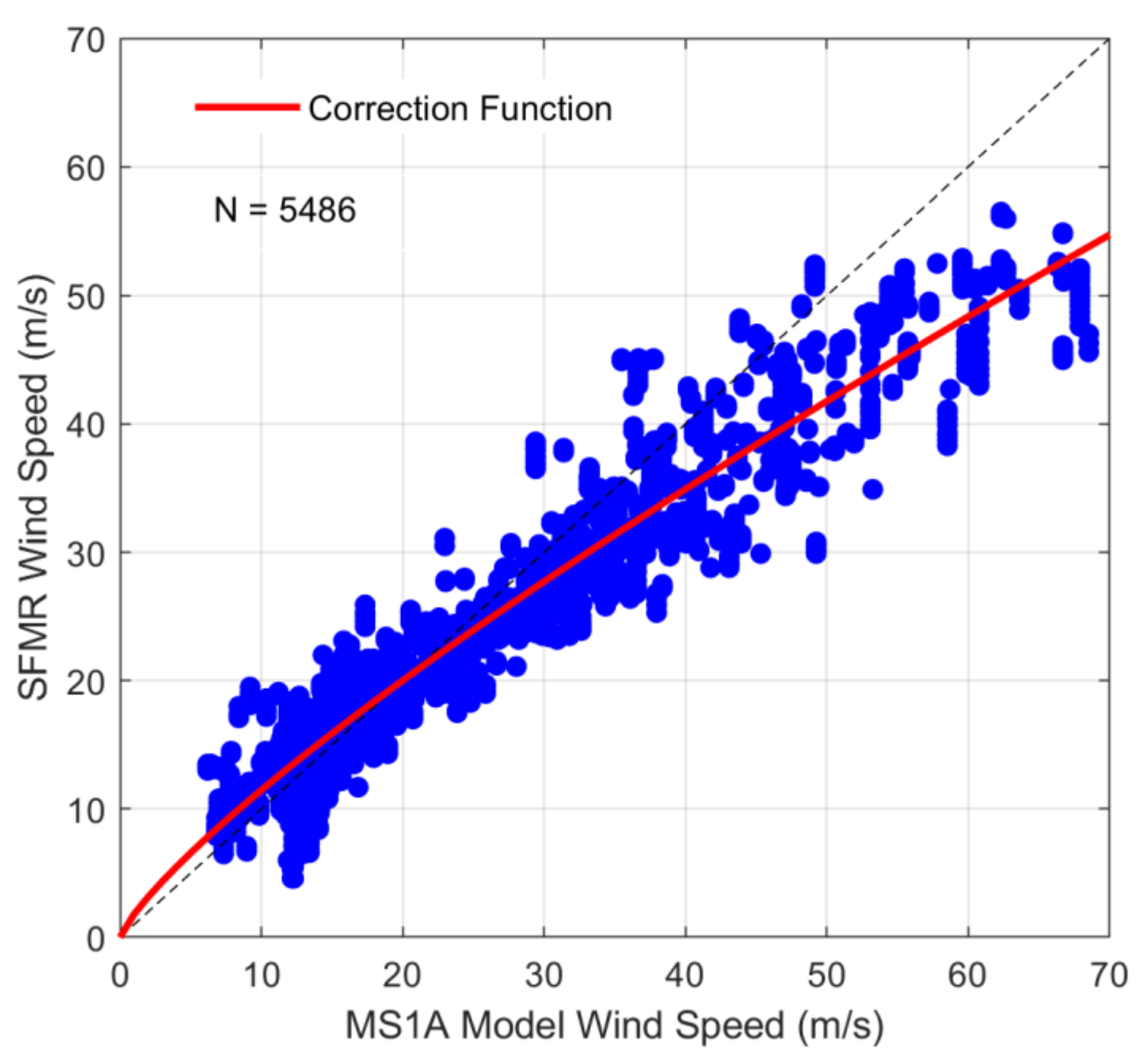
The surface wind speeds retrieved by the MS1A model were compared with the SFMR measurements, as shown in Figure 3 and Table 2. There were 5486 collocations in total. We defined the averaged bias as follows:
where the is the wind speed retrieval, the is the wind speed reference. The unit is meter per second. N stands for the total collocation number. For all collocations, the averaged bias, correlation coefficient (Cor) and root mean-square error (RMSE) are 1.46 m/s, 0.96 and 4.68 m/s, respectively. Although the retrievals are highly correlated with the SFMR data, the averaged bias increases from negative to positive with increasing wind speed, indicating that the MS1A model underestimates low-to-moderate wind speeds slightly and overestimates high-to-extreme wind speeds dramatically. The reason for overestimation is the different relationships between VH NRCS and wind speeds from SMAP and SFMR. According to the Figure 3 in [31], for one VH NRCS value in the high-to-extreme wind regime, the SMAP provides higher wind speeds than SFMR.
The correction function illustrated with the red curve in Figure 3 was fitted from 6 to 69 m/s:
where and are the MS1A-retrieved wind speeds after and before modification, respectively. The unit is meter per second. According to this function, the modified result is 54.74 m/s for the original 70 m/s. Figure 4 shows the wind retrievals after modification. Compared with the retrievals shown in Figure 2, extreme wind speeds had been reduced evidently and low-to-moderate wind speeds were increased slightly. To note, due to the quantitative limitation of SFMR collocations, we were neither able to refine the MS1A model for each sub-swath individually, nor validate it using other SFMR data.
4. TC Intensity Parameters Retrieval
4.1. Surface Maximum Wind Speed
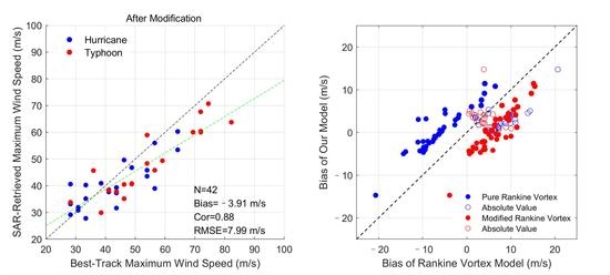
In order to evaluate the modified MS1A model and the relationships between intensity parameters, we retrieved the sea surface wind fields of 42 TC samples with the original MS1A model and the modified MS1A model separately. Then, maximum wind speeds were extracted for each sample. The maximum winds before and after modification were validated with those provided by best-tracks, as shown in Figure 5. The green dashed lines illustrate the trends of point distribution. For all samples, best-track maximum winds ranged from 55 to 160 knots, i.e., 28.27 to 82.24 m/s. The Typhoon Halong (2019) developed over the western Pacific Ocean had the highest maximum wind speed.
For the retrievals before modification, the averaged bias, Cor and RMSE are 5.96 m/s, 0.88 and 9.99 m/s, respectively. The MS1A model overestimated the maximum wind speeds for most samples. After modification, retrievals matched best-track data much better, the averaged bias, Cor and RMSE are −3.91 m/s, 0.88 and 7.99 m/s. Results demonstrate that the retrieval bias and RMSE of the MS1A model are corrected by the modification function effectively. Last but not least, averaged biases of −2.12 and −6.08 m/s are reported for hurricanes and typhoons respectively, which were possibly caused by the different wind speed ranges of samples.
High wind in TC inner core is always accompanied by heavy precipitation. As previous studies confirmed, the contribution of extreme rainfall is difficult to be removed from the backscattered signal, since the C-band signal has ambiguous behavior to rainfall and the collocated high-spatial-resolution rainfall measurements are generally unavailable [33,34]. As a result, maximum wind speed is difficult to be retrieved accurately [31,32,35,36]. In addition, best-tracks are known to be particularly limited in the situation that TC evolves fast [37,38,39,40]. It should be noted that our work does not consider different rainfall situations and intensity evolutions. The discrepancies in Figure 3 and Figure 5 are possibly induced by the two issues mentioned above.
4.2. Tropical Cyclone Fullness
As mentioned previously, the TCF value relates to the size parameters and maximum wind speed, written as:
After determining the center location, RMW could be derived from the point with the maximum wind speed in a retrieval map. This parameter has been proven to be a more reliable information than maximum wind speed, due to the strong reflectivity of the signal and as it is less subject to time-averaged convention and less affected by disturbances such as heavy precipitations [28].
Radial wind fitting was utilized to extract R17, based on the distribution of wind retrievals in a different radius. Figure 6 shows an example of the Hurricane Michael’s wind distribution within 200 km, acquired at 23:43 UTC, 9 October 2018. The wind distribution from 19 to 200 km was fitted by a power function and shown in black curve, i.e., a radial wind curve. We calculated R17 according to this curve and finally got the TCF value with Equation (3). For this case, the RMW, R17 and TCF are 19.0 km, 157.5 km and 0.88, respectively.
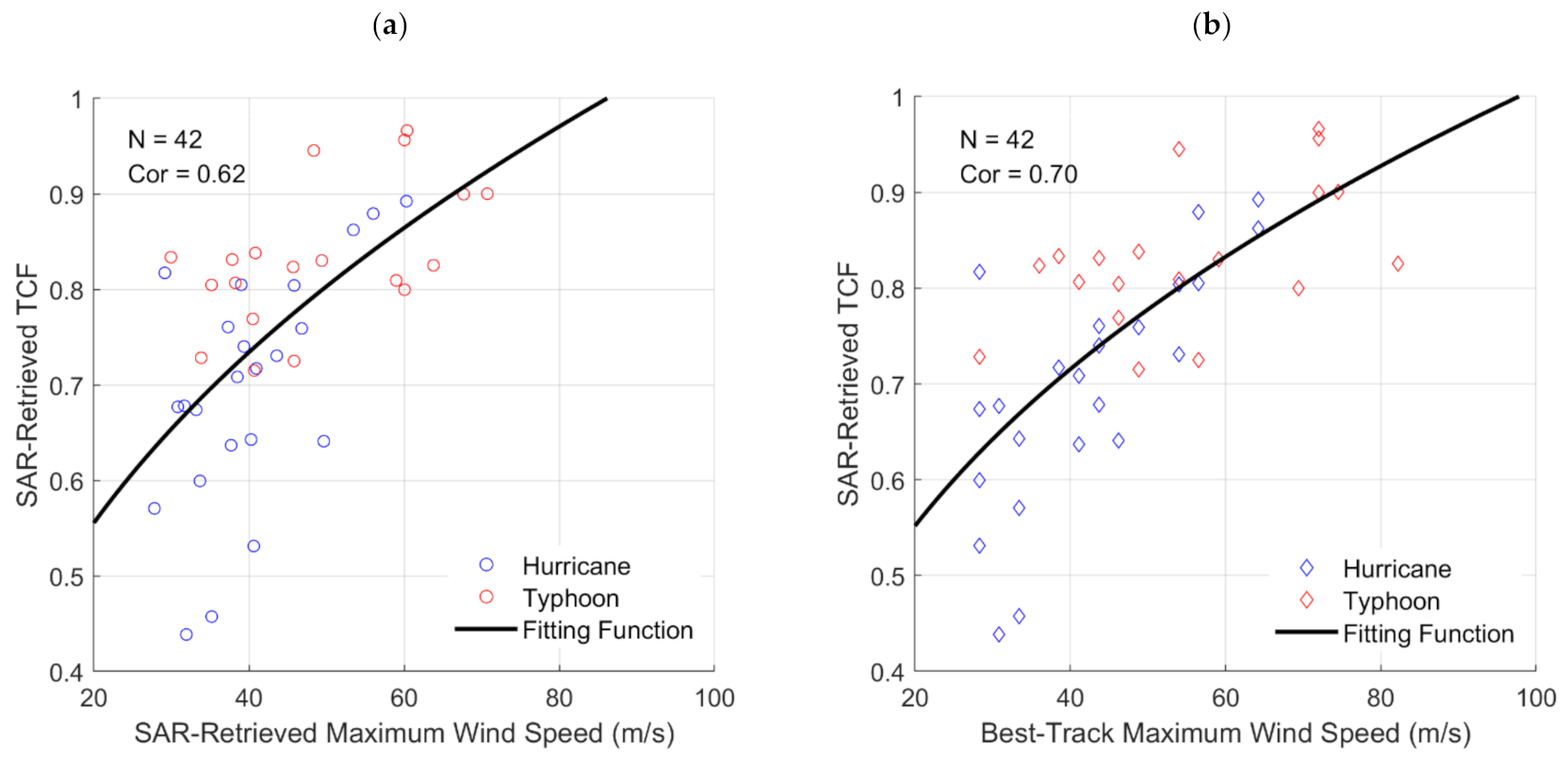
According to the methodology above, the TCF values of 42 TC samples were calculated and compared with the SAR-retrieved maximum wind speeds and the best-track maximum wind speeds. Results are shown in Figure 7. The TCF value increases with increasing maximum wind speed. The Cor between the TCF values and the SAR-retrieved maximum winds is 0.62, lower than that of the best-track maximum winds (0.70). Finally, empirical equations of the two intensity parameters were presented as follows:
where stands for the maximum wind speeds retrieved by the modified MS1A model, and stands for the maximum wind speeds collected from best-track data. The two equations just have minor differences in coefficients, because the maximum winds from the two sources match well.
4.3. Central Surface Pressure
The Holland hurricane model describes the symmetric radial profiles of sea surface pressure and wind speed for TCs [7]. When the maximum wind speed (), RMW, central surface pressure () and ambient pressure (= 1010 mb) are given, surface wind speed could be calculated by:
where is 10-m wind speed in meter per second. r is the distance from TC center in meter. B is the shape parameter. = 1.15 kg m−3 is air density. e = 2.7183. f is the Coriolis parameter and is the latitude of TC center. After inputting = 17 m/s, R17 and Equation (3) into the Equation (6), the Holland model is rewritten as:
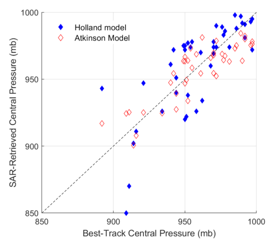
According the Equation (9), we calculated the central surface pressures of all TC samples and validated the results with best-track data. Comparison is illustrated in Figure 8 (blue diamond) and Table 3. Pressure retrievals vary from about 850 to 1000 mb. The averaged bias, Cor and RMSE between the pressures of two sources are 1.17 mb, 0.77 and 21.29 mb.
In addition, according to the Atkinson wind-pressure model, i.e., the Equation (10), we calculated the central surface pressures and compared them with those provided by best-tracks. The results are shown in Figure 8 (red unfilled diamond) and Table 3. The averaged bias, Cor and RMSE between the two sources’ pressures are −2.64 mb, 0.86 and 13.54 mb. Although the computation of the Holland model used more parameters, its results just have a smaller bias than the Atkinson model. For the latter model, Cor and RMSE are better than the former model.
5. Wind Field Model Development
In a TC weather system, surface wind speed generally increases from center to eyewall and decreases from the eyewall to the outer regions. Maximum wind speed appears near the eyewall. Intensity and size are two key factors for forecasting and studying TCs. As a consequence, a large number of wind field models have been developed to simulate TC wind distribution, based on limited observations; for example, , and RMW. Many studies bring size parameters from observations or use some peripheric information to improve the model accuracy [8,41,42]. However, they did not benefit from high-resolution data like SAR retrievals.
In this study, we combined the radial wind curve, the Rankine Vortex model [43] and the relationship between TCF and to propose a new TC wind field model. By this model, wind field could be calculated symmetrically with and RMW. Wind field size was considered as the TCF value relating RMW, R17 and . When rRMW, we used the following power function to describe wind profile:
where the unit of r and RMW is kilometers. To determine the coefficients a and b, we brought (RMW,) and (R17,17) into Equation (11) and got:
After solving them, we got:
where the TCF value could be computed by the Equation (4) or (5). According to the Equation (12), a was expressed as:
As a result, the coefficients a and b are the functions of and RMW. Wind speed at radius r can be calculated using the Equation (11) if and RMW are known. It should be noted that the new model could be only used within a 200-km radius, because only the radial wind curve had been investigated in this region.
For rRMW, we used the Rankine Vortex model to calculate wind speed:
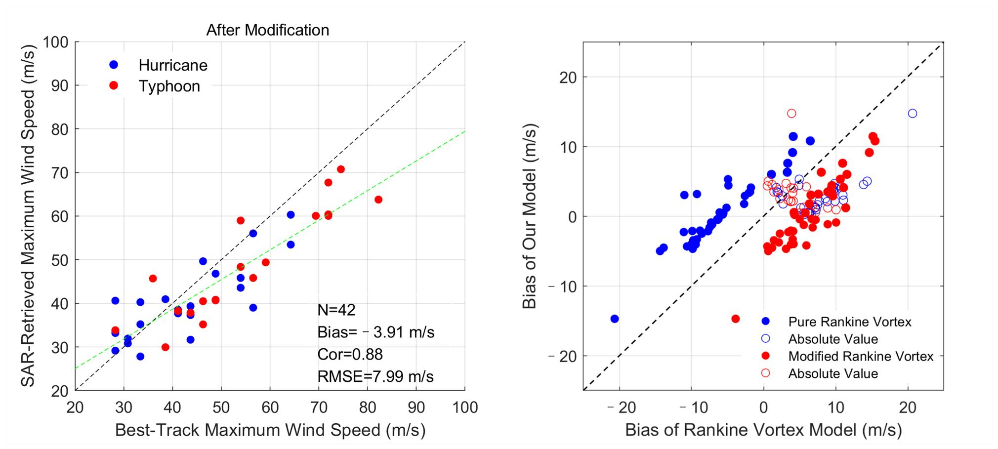
In order to evaluate the proposed model, we inputted all the TC samples’ maximum wind speeds and RMW values into the new model and the Rankine Vortex model to simulate wind fields within the 200-km radius. For rRMW, the Rankine Vortex model is expressed as:
where is the decay component. For the pure situation, = 1. Considering different categories, the modified Rankine Vortex statistics in [43] illustrate different values.
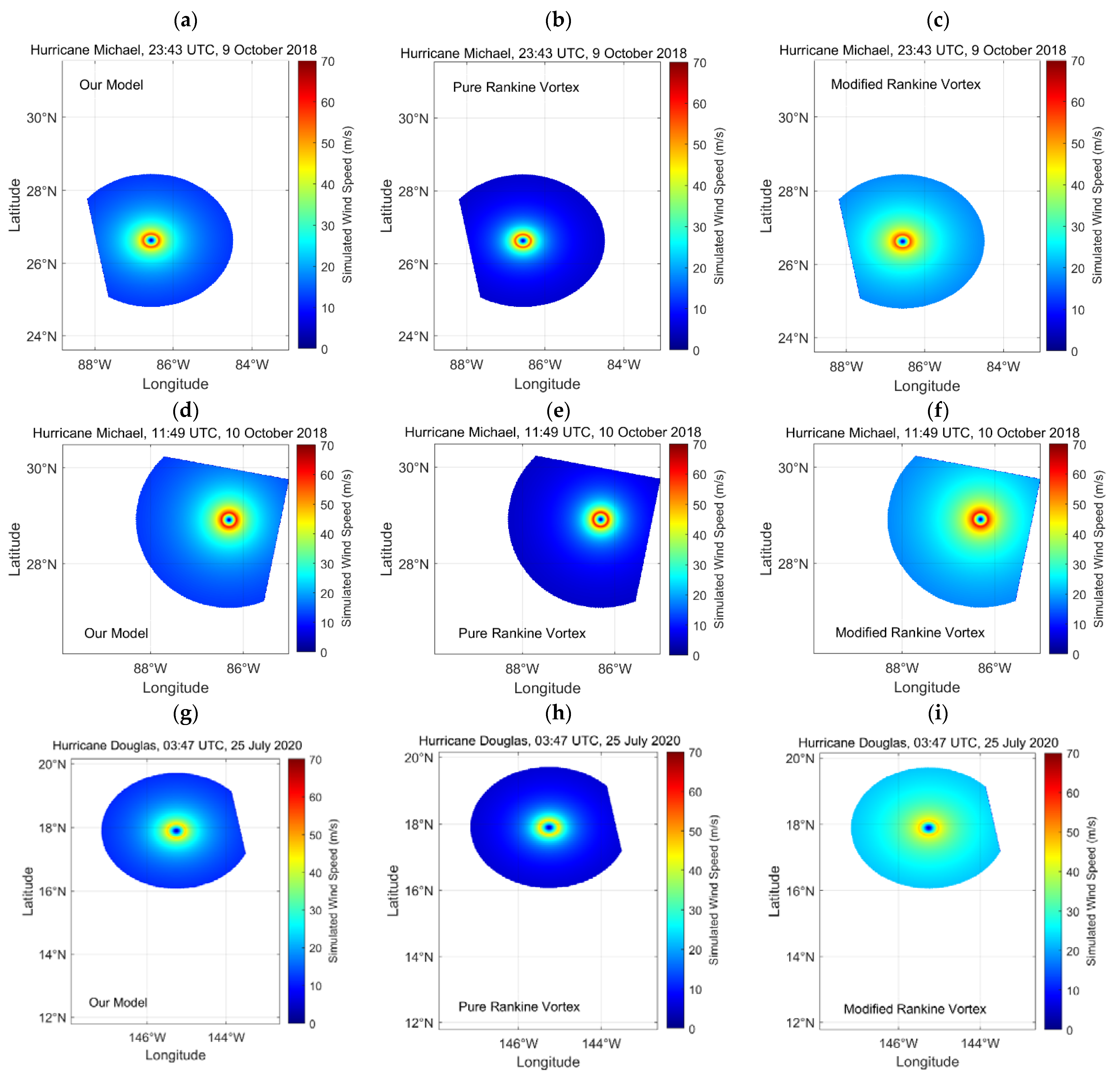
For the hurricane samples presented in Table 1, Figure 9 shows the wind speeds simulated by our model (left column) and those simulated by the pure Rankine Vortex model (middle column) and the modified Rankine Vortex model (right column). The simulations of our model are larger than those of the pure Rankine Vortex model, smaller than those of the modified Rankine Vortex model and more similar to retrievals.
All simulations were compared statistically with the retrievals of the modified MS1A model. The averaged bias, averaged absolute bias and averaged RMSE were computed using the following equations:
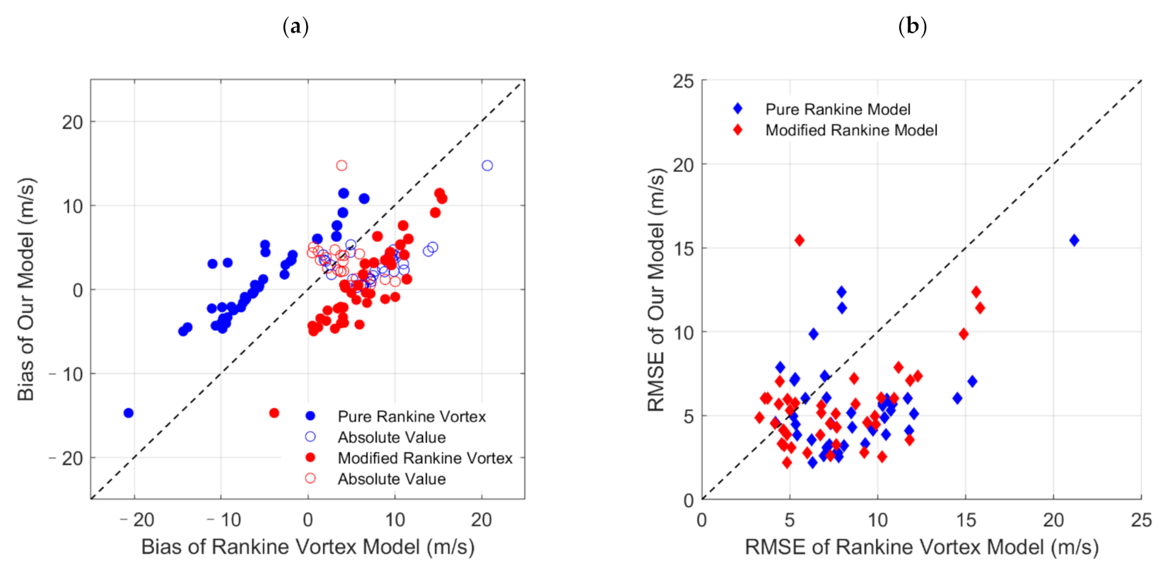
where and stand for the simulated wind speeds and retrieved wind speeds. is the point number of a TC sample and = 42. Comparisons of the two models are illustrated in Figure 10 and Table 4. For the pure Rankine model, , and are −6.25, 7.31 and 8.72 m/s, respectively. For the modified Rankine model, , and are 6.47, 6.65 and 7.67 m/s, respectively. For more samples, our model performs better than the Rankine models. Its , and are 0.27, 3.78 and 5.52 m/s, respectively.
6. Discussion
In this study, TCs’ maximum wind speeds, central surface pressures and TCF values were retrieved from SAR images according to several methodologies, for example the modified MS1A GMF, the Holland hurricane model, the Atkinson wind-pressure model, radial wind profile fitting and the definition of TCF. Among them, the modified MS1A model was fundamental, because three intensity parameters were derived from wind retrievals directly or indirectly. In GMF modification, the MS1A retrievals were compared with the AOML/HRD SFMR winds. This retrieval was previously compared to STAR/NESDIS SFMR winds [32], which are approximately 5 m/s higher than AOML/HRD SFMR winds, due to different solutions to remove rain contamination in wind speed estimates [44]. It will be interesting to refine MS1A with a different SFMR product.
As a part of the evaluation, the retrieved maximum wind speeds had been compared with those collected from best-tracks and are shown in Figure 5b. One possible error source was that the best-track maximum wind speeds were time-averaged; however, the maximum wind speeds retrieved from SAR images were at certain moments. As a consequence, all equations in this paper containing or possibly have an error if the best-track maximum wind speeds are inputs.
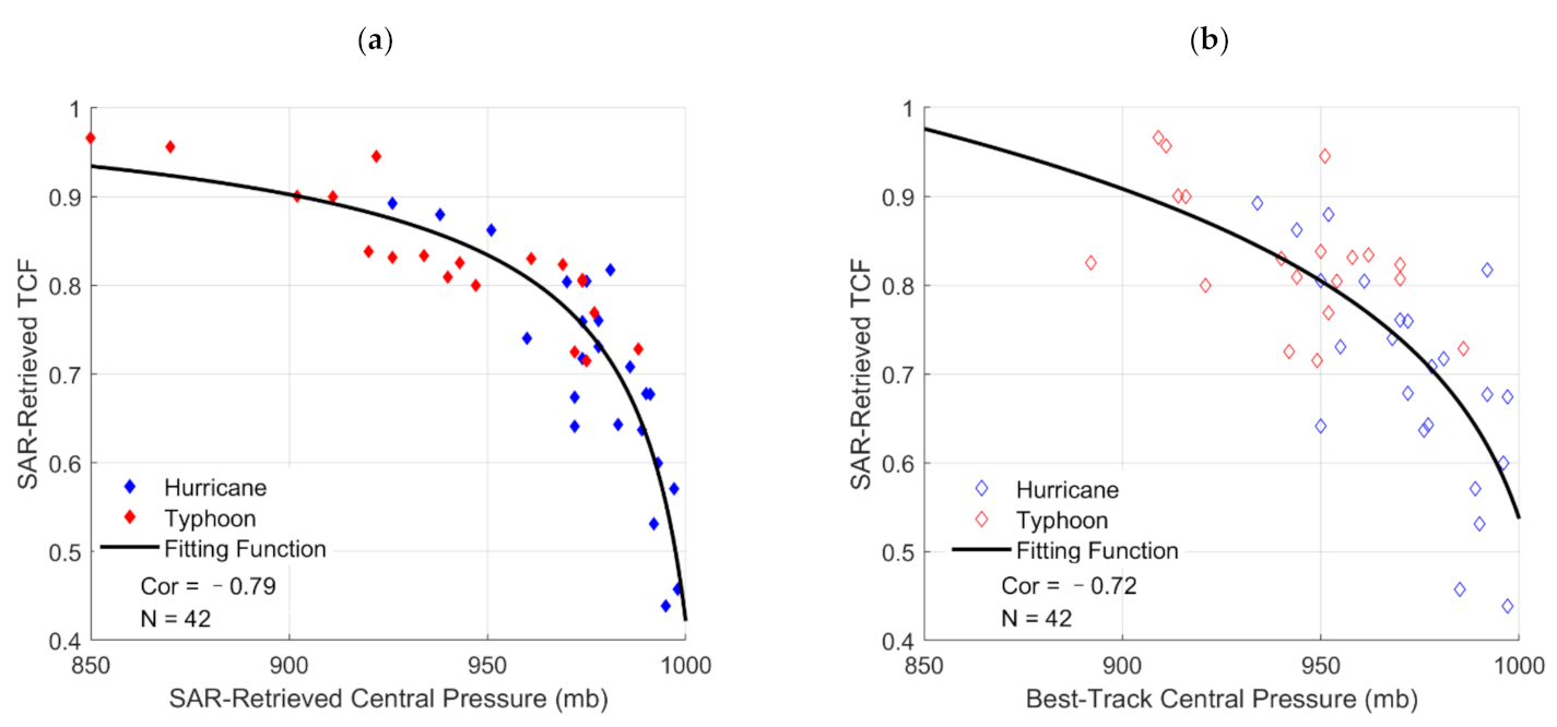
Investigating the relationships between intensity parameters is one aim of this study. Figure 11 shows the distributions of SAR-retrieved maximum wind speeds, central pressures using the Holland hurricane model () and pressures provided by best-tracks (). Figure 12 shows the distributions of SAR-retrieved TCF values and the central pressures of two sources.
Pressure is negatively dependent on the other two intensity parameters. Based on these relationships, we proposed four empirical functions:
It should be noted that the pressure ranges are 850–1000 mb for and 892–1000 mb for .
7. Conclusions
Sea surface wind field structure and intensity variation are hot topics in TC study. This paper focused on the added-value of C-band SAR cross-polarization images for retrieving TC intensity parameters, which include maximum wind speed, central surface pressure and TC fullness, and on developing a wind field model.
GMF plays an important role in retrieving intensity and size information. Thus, we first modified the MS1A model to improve its retrieval accuracy in an extreme wind regime at a high spatial resolution. The SFMR wind data of two hurricanes were collected and matched with 1-km wind speeds retrieved by the MS1A model from the Sentinel-1A images after location shift. Matching results up to 69 m/s indicated that the MS1A model overestimated winds and the bias increased when wind speeds exceeded 20 m/s. Based on power fitting, a modification function was proposed to correct MS1A’s retrieval bias.
For validation and comparison, we retrieved 42 TC samples’ wind speeds using the MS1A model before and after the modification. These TCs’ intensities varied from a tropical storm to category 5. The comparison between SAR-retrieved maximum winds and those collected from best-tracks indicated that the MS1A model had a better performance after the modification. The averaged retrieval bias, Cor and RMSE are –3.91 m/s, 0.88 and 7.99 m/s, respectively.
Based on the 1-km SAR-retrieved wind fields, we studied the relationship between maximum wind speed and size parameters which were related by TCF. The values of R17 and RMW were derived from radial wind curves fitted by power function. Comparison between the TCF values and maximum wind speeds showed that they had a positive correlation. Two empirical functions of TCF and maximum wind speed were proposed based on SAR retrievals and best-track data.
An experiment was carried out to retrieve all TC samples’ central pressures by the Holland hurricane model and the Atkinson wind-pressure model from wind retrievals. The values of R17 and TCF were inputted into the Holland model for calculation with a single equation. Compared with best-track pressures, the Holland model’s results have a smaller bias, the Atkinson model’s results have a larger Cor and a smaller RMSE.
In addition, we combined the proposed wind-TCF function, the Rankine Vortex model and the radial wind curve to develop a new wind field model. For the regions of radius larger than RMW, the model was designed with a power function, whose form is the same as the function used for fitting the radial wind curve. Two coefficients were determined by the values of RMW and maximum wind speed and 42 samples’ simulations demonstrated that the proposed model had a better performance than the pure and modified Rankine Vortex models in the aspects of averaged bias, averaged absolute bias and averaged RMSE.
Finally, the SFMR product and error source were discussed. The impact of time-averaged maximum winds from best-tracks might lead to an error when SAR-retrieved intensity parameters were compared with them and in some empirical functions we proposed. In addition, the relationships between central surface pressure and the other two intensity parameters were analyzed and applied to empirical function development.
Author Contributions
Initiation of the idea: Y.G.; Data processing and model proposing: Y.G.; Writing and editing: all authors contributed; Supervision: J.Z.; Funding acquisition: J.Z., J.S., and C.G. All authors have read and agreed to the published version of the manuscript.
Funding
This research was funded by the National Science Foundation of China under grants 61931025, U20A2099, and 41976017, the Fundamental Research Funds for the Central Universities under grant 20CX06109A, the Qingdao Postdoctoral Foundation Funded Project under grant qdyy20200098.
Institutional Review Board Statement
Not applicable.
Informed Consent Statement
Not applicable.
Data Availability Statement
The data used in this study are available on request from the author.
Acknowledgments
We thank the European Space Agency for making the Sentinel-1 data publicly available. We thank the Hurricane Research Division of National Oceanic and Atmospheric Administration for SFMR data and hurricane best-tracks, the Joint Typhoon Warning Center for typhoon best-tracks.
Conflicts of Interest
The authors declare no conflict of interest.
Appendix A
In this section, TC samples and their SAR data information are briefly listed in Table A1 and Table A2. Corresponding best-track data, e.g., center locations, maximum winds and central surface pressures are not shown here but available on request from the author.

Table A1.
Brief information of 19 typhoon samples and SAR images used in this study.
| Typhoon | |||
|---|---|---|---|
| Name | Area | SAR Instrument | Acquisition Time (UTC) |
| Megi | Western Pacific | Sentinel-1A | 20160926 09:34 |
| Jongdari | Western Pacific | Sentinel-1B | 20180725 20:46 |
| Sentinel-1A | 20180726 20:37 | ||
| Sentinel-1B | 20180727 08:22 | ||
| Shanshan | Western Pacific | Sentinel-1A | 20180808 08:23 |
| Soulik | Western Pacific | Sentinel-1B | 20180818 08:38 |
| 20180818 20:45 | |||
| Jebi | Western Pacific | Sentinel-1B | 20180829 07:55 |
| Sentinel-1A | 20180831 20:39 | ||
| Mangkhut | Western Pacific | Sentinel-1B | 20180911 20:47 |
| Sentinel-1A | 20180914 09:50 | ||
| Trami | Western Pacific | Sentinel-1A | 20180925 21:20 |
| 20180928 09:35 | |||
| Kon-Rey | Western Pacific | Sentinel-1A | 20181002 21:11 |
| Yutu | Western Pacific | Sentinel-1A | 20181025 20:31 |
| Hagibis | Western Pacific | Sentinel-1A | 20191008 20:30 |
| Halong | Western Pacific | Sentinel-1A | 20191105 19:57 |
| Sentinel-1B | 20191106 19:49 | ||
| Sentinel-1A | 20191107 19:39 | ||
Table A2.
Brief information of 23 hurricane samples and SAR images used in this study.
| Hurricane | |||
|---|---|---|---|
| Name | Area | SAR Instrument | Acquisition Time (UTC) |
| Lester | East Pacific | Sentinel-1A | 20160826 13:39 |
| 20160830 14:45 | |||
| 20160831 03:15 | |||
| Gaston | Atlantic | Sentinel-1A | 20160826 21:16 |
| 20160827 09:21 | |||
| 20160829 21:41 | |||
| 20160830 09:45 | |||
| 20160901 20:29 | |||
| Hermine | Atlantic | Sentinel-1A | 20160904 22:32 |
| Karl | Atlantic | Sentinel-1A | 20160923 22:22 |
| Miriam | East Pacific | Sentinel-1A | 20180831 03:32 |
| Florence | Atlantic | Sentinel-1A | 20180904 08:34 |
| 20180908 09:39 | |||
| Helene | Atlantic | Sentinel-1B | 20180912 08:18 |
| Sergio | East Pacific | Sentinel-1A | 20181006 14:06 |
| 20181007 02:34 | |||
| 20181009 14:29 | |||
| Michael | Atlantic | Sentinel-1A | 20181009 23:43 |
| 20181010 11:49 | |||
| Leslie | Atlantic | Sentinel-1A | 20181013 07:15 |
| Juliette | East Pacific | Sentinel-1A | 20190904 13:39 |
| Douglas | East Pacific | Sentinel-1A | 20200725 03:47 |
| Teddy | Atlantic | Sentinel-1A | 20200922 10:16 |
References
- Katsaros, K.B.; Vachon, P.W.; Liu, W.T.; Black, P.G. Microwave Remote Sensing of Tropical Cyclones from Space. J. Oceanogr. 2002, 58, 137–151. [Google Scholar] [CrossRef]
- Kossin, J.P. Hurricane Wind–Pressure Relationship and Eyewall Replacement Cycles. Weather Forecast. 2015, 30, 177–181. [Google Scholar] [CrossRef]
- Guo, X.; Tan, Z.-M. Tropical cyclone fullness: A new concept for interpreting storm intensity. Geophys. Res. Lett. 2017, 44, 4324–4331. [Google Scholar] [CrossRef]
- Simpson, R.H.; Saffir, H. The hurricane disaster-potential scale. Weatherwise 1974, 27, 186. [Google Scholar]
- Knaff, J.A.; Zehr, R.M. Reexamination of Tropical Cyclone Wind–Pressure Relationships. Weather Forecast. 2006, 22, 71–88. [Google Scholar] [CrossRef]
- Xie, L.; Bao, S.; Pietrafesa, L.J.; Foley, K.; Fuentes, M. A Real-Time Hurricane Surface Wind Forecasting Model: Formulation and Verification. Mon. Weather Rev. 2006, 134, 1355–1370. [Google Scholar] [CrossRef]
- Holland, G.J. An Analytic Model of the Wind and Pressure Profiles in Hurricanes. Mon. Weather Rev. 1980, 108, 1212–1218. [Google Scholar] [CrossRef]
- Holland, G.J.; Belanger, J.I.; Fritz, A. A Revised Model for Radial Profiles of Hurricane Winds. Mon. Weather Rev. 2010, 138, 4393–4401. [Google Scholar] [CrossRef]
- Merrill, R.T. A Comparison of Large and Small Tropical Cyclones. Mon. Weather Rev. 1984, 112, 1408–1418. [Google Scholar] [CrossRef] [Green Version]
- Hill, K.A.; Lackmann, G.M. Influence of Environmental Humidity on Tropical Cyclone Size. Mon. Weather Rev. 2009, 137, 3294–3315. [Google Scholar] [CrossRef]
- Chan, K.T.F.; Chan, J.C.L. Size and Strength of Tropical Cyclones as Inferred from QuikSCAT Data. Mon. Weather Rev. 2012, 140, 811–824. [Google Scholar] [CrossRef]
- Yu, P.; Johannessen, J.A.; Yan, X.-H.; Geng, X.; Zhong, X.; Zhu, L. A Study of the Intensity of Tropical Cyclone Idai Using Dual-Polarization Sentinel-1 Data. Remote Sens. 2019, 11, 2837. [Google Scholar] [CrossRef] [Green Version]
- Li, X.; Zhang, J.; Yang, X.; Pichel, W.G.; DeMaria, M.; Long, D.; Li, Z. Tropical Cyclone Morphology from Spaceborne Synthetic Aperture Radar. Bull. Am. Meteorol. Soc. 2013, 94, 215–230. [Google Scholar] [CrossRef] [Green Version]
- Klotz, B.W.; Jiang, H. Global composites of surface wind speeds in tropical cyclones based on a 12 year scatterometer database. Geophys. Res. Lett. 2016, 43, 480–488. [Google Scholar] [CrossRef]
- Shao, W.; Yuan, X.; Sheng, Y.; Sun, J.; Zhou, W.; Zhang, Q. Development of Wind Speed Retrieval from Cross-Polarization Chinese Gaofen-3 Synthetic Aperture Radar in Typhoons. Sensors 2018, 18, 412. [Google Scholar] [CrossRef] [Green Version]
- Horstmann, J.; Falchetti, S.; Wackerman, C.; Maresca, S.; Caruso, M.J.; Graber, H.C. Tropical Cyclone Winds Retrieved From C-Band Cross-Polarized Synthetic Aperture Radar. IEEE Trans. Geosci. Remote Sens. 2015, 53, 2887–2898. [Google Scholar] [CrossRef] [Green Version]
- Gao, Y.; Guan, C.; Sun, J.; Xie, L. Tropical Cyclone Wind Speed Retrieval from Dual-Polarization Sentinel-1 EW Mode Products. J. Atmos. Ocean. Technol. 2020, 37, 1713–1724. [Google Scholar] [CrossRef]
- Shao, W.; Li, X.; Hwang, P.; Zhang, B.; Yang, X. Bridging the gap between cyclone wind and wave by C -band SAR measurements. J. Geophys. Res. Oceans 2017, 122, 6714–6724. [Google Scholar] [CrossRef]
- Hwang, P.A.; Zhang, B.; Perrie, W. Depolarized radar return for breaking wave measurement and hurricane wind retrieval. Geophys. Res. Lett. 2010, 37, 70–75. [Google Scholar] [CrossRef]
- Phillips, O.M. Radar Returns from the Sea Surface—Bragg Scattering and Breaking Waves. J. Phys. Oceanogr. 1988, 18, 1065–1074. [Google Scholar] [CrossRef]
- Zhang, B.; Perrie, W. Cross-Polarized Synthetic Aperture Radar: A New Potential Measurement Technique for Hurricanes. Bull. Am. Meteorol. Soc. 2012, 93, 531–541. [Google Scholar] [CrossRef] [Green Version]
- Zhang, G.; Perrie, W.; Zhang, B.; Yang, J.; He, Y. Monitoring of tropical cyclone structures in ten years of RADARSAT-2 SAR images. Remote Sens. Environ. 2020, 236, 111449. [Google Scholar] [CrossRef]
- Gao, Y.; Guan, C.; Sun, J.; Xie, L. A Wind Speed Retrieval Model for Sentinel-1A EW Mode Cross-Polarization Images. Remote Sens. 2019, 11, 153. [Google Scholar] [CrossRef] [Green Version]
- Zhang, G.; Li, X.; Perrie, W.; Hwang, P.A.; Zhang, B.; Yang, X. A Hurricane Wind Speed Retrieval Model for C-Band RADARSAT-2 Cross-Polarization ScanSAR Images. IEEE Trans. Geosci. Remote Sens. 2017, 55, 4766–4774. [Google Scholar] [CrossRef]
- Hwang, P.A.; Stoffelen, A.; van Zadelhoff, G.-J.; Perrie, W.; Zhang, B.; Li, H.; Shen, H. Cross-polarization geophysical model function for C-band radar backscattering from the ocean surface and wind speed retrieval. J. Geophys. Res. Oceans 2015, 120, 893–909. [Google Scholar] [CrossRef]
- Mouche, A.A.; Chapron, B.; Zhang, B.; Husson, R. Combined Co- and Cross-Polarized SAR Measurements Under Extreme Wind Conditions. IEEE Trans. Geosci. Remote Sens. 2017, 55, 6746–6755. [Google Scholar] [CrossRef]
- Meissner, T.; Ricciardulli, L.; Wentz, F.J. Capability of the SMAP Mission to Measure Ocean Surface Winds in Storms. Bull. Am. Meteorol. Soc. 2017, 98, 1660–1677. [Google Scholar] [CrossRef]
- Combot, C.; Mouche, A.; Knaff, J.; Zhao, Y.; Zhao, Y.; Vinour, L.; Quilfen, Y.; Chapron, B. Extensive High-Resolution Synthetic Aperture Radar (SAR) Data Analysis of Tropical Cyclones: Comparisons with SFMR Flights and Best Track. Mon. Weather Rev. 2020, 148, 4545–4563. [Google Scholar] [CrossRef]
- Uhlhorn, E.W.; Black, P.G.; Franklin, J.L.; Goodberlet, M.; Carswell, J.; Goldstein, A.S. Hurricane Surface Wind Measurements from an Operational Stepped Frequency Microwave Radiometer. Mon. Weather Rev. 2007, 135, 3070–3085. [Google Scholar] [CrossRef] [Green Version]
- Klotz, B.W.; Uhlhorn, E.W. Improved Stepped Frequency Microwave Radiometer Tropical Cyclone Surface Winds in Heavy Precipitation. J. Atmos. Ocean. Technol. 2014, 31, 2392–2408. [Google Scholar] [CrossRef]
- Gao, Y.; Sun, J.; Zhang, J.; Guan, C. Extreme Wind Speeds Retrieval Using Sentinel-1 IW Mode SAR Data. Remote Sens. 2021, 13, 1867. [Google Scholar] [CrossRef]
- Mouche, A.; Chapron, B.; Knaff, J.; Zhao, Y.; Zhang, B.; Combot, C. Copolarized and Cross-Polarized SAR Measurements for High-Resolution Description of Major Hurricane Wind Structures: Application to Irma Category 5 Hurricane. J. Geophys. Res. Oceans 2019, 124, 3905–3922. [Google Scholar] [CrossRef]
- Alpers, W.; Zhang, B.; Mouche, A.; Zeng, K.; Chan, P.W. Rain footprints on C-band synthetic aperture radar images of the ocean—Revisited. Remote Sens. Environ. 2016, 187, 169–185. [Google Scholar] [CrossRef]
- Katsaros, K.; Vachon, P.W.; Black, P.; Dodge, P.; Uhlhorn, E. Wind Fields from SAR: Could They Improve Our Understanding of Storm Dynamics? Johns Hopkins APL Tech. Dig. 2000, 21, 86–93. [Google Scholar] [CrossRef] [Green Version]
- Reppucci, A.; Lehner, S.; Schulz-Stellenfleth, J.; Brusch, S. Tropical Cyclone Intensity Estimated From Wide-Swath SAR Images. IEEE Trans. Geosci. Remote Sens. 2010, 48, 1639–1649. [Google Scholar] [CrossRef]
- Xu, F.; Li, X.; Wang, P.; Yang, J.; Pichel, W.G.; Jin, Y.-Q. A Backscattering Model of Rainfall Over Rough Sea Surface for Synthetic Aperture Radar. IEEE Trans. Geosci. Remote Sens. 2014, 53, 3042–3054. [Google Scholar] [CrossRef]
- Velden, C.; Harper, B.; Wells, F.; Beven, J.L.; Zehr, R.; Olander, T.; Mayfield, M.; Guard, C.; Lander, M.; Edson, R.; et al. Supplement To: The Dvorak Tropical Cyclone Intensity Estimation Technique: A Satellite-Based Method that Has Endured for over 30 Years. Bull. Am. Meteorol. Soc. 2006, 87, S6–S9. [Google Scholar] [CrossRef]
- Rappaport, E.N.; Jiing, J.-G.; Landsea, C.W.; Murillo, S.T.; Franklin, J.L. The Joint Hurricane Test Bed: Its First Decade of Tropical Cyclone Research-To-Operations Activities Reviewed. Bull. Am. Meteorol. Soc. 2012, 93, 371–380. [Google Scholar] [CrossRef] [Green Version]
- Carrasco, C.A.; Landsea, C.W.; Lin, Y.-L. The Influence of Tropical Cyclone Size on Its Intensification. Weather Forecast. 2014, 29, 582–590. [Google Scholar] [CrossRef] [Green Version]
- Leroux, M.-D.; Meister, J.; Mekies, D.; Dorla, A.-L.; Caroff, P. A Climatology of Southwest Indian Ocean Tropical Systems: Their Number, Tracks, Impacts, Sizes, Empirical Maximum Potential Intensity, and Intensity Changes. J. Appl. Meteorol. Clim. 2018, 57, 1021–1041. [Google Scholar] [CrossRef]
- Knaff, J.A.; Sampson, C.R.; DeMaria, M.; Marchok, T.P.; Gross, J.M.; McAdie, C.J. Statistical Tropical Cyclone Wind Radii Prediction Using Climatology and Persistence. Weather Forecast. 2005, 22, 781–791. [Google Scholar] [CrossRef]
- Rappin, E.D.; Nolan, D.S.; Majumdar, S.J. A Highly Configurable Vortex Initialization Method for Tropical Cyclones. Mon. Weather Rev. 2013, 141, 3556–3575. [Google Scholar] [CrossRef]
- Mallen, K.J.; Montgomery, M.T.; Wang, B. Reexamining the Near-Core Radial Structure of the Tropical Cyclone Primary Circulation: Implications for Vortex Resiliency. J. Atmos. Sci. 2005, 62, 408–425. [Google Scholar] [CrossRef] [Green Version]
- Sapp, J.W.; Alsweiss, S.O.; Jelenak, Z.; Chang, P.S.; Carswell, J. Stepped Frequency Microwave Radiometer Wind-Speed Retrieval Improvements. Remote Sens. 2019, 11, 214. [Google Scholar] [CrossRef] [Green Version]
Figure 1.
The numbers of the TC samples we used in different categories and different sea areas.

Figure 2.
The Sentinel-1A EW mode cross-polarization images of (a) the Hurricane Michael at 23:43 UTC, 9 October 2018, (b) the Hurricane Michael at 11:49 UTC, 10 October 2018, (c) the Hurricane Douglas the Hurricane Michael at 03:47 UTC, 25 July 2020. (d), (e), (f) are the corresponding MS1A-retrieved sea surface wind speeds of (a), (b), (c) used for MS1A modification.

Figure 3.
Comparison between the MS1A-retrieved and the SFMR-measured wind speeds, according to the samples of the Hurricane Michael and the Hurricane Douglas. The red curve fitted stands for the correction function of the MS1A model.
Figure 3.
Comparison between the MS1A-retrieved and the SFMR-measured wind speeds, according to the samples of the Hurricane Michael and the Hurricane Douglas. The red curve fitted stands for the correction function of the MS1A model.

Figure 4.
Sea surface wind speeds retrieved by the modified MS1A model for (a) the Hurricane Michael on 9 October 2018, (b) the Hurricane Michael on 10 October 2018, (c) the Hurricane Douglas on 25 July 2020.
Figure 4.
Sea surface wind speeds retrieved by the modified MS1A model for (a) the Hurricane Michael on 9 October 2018, (b) the Hurricane Michael on 10 October 2018, (c) the Hurricane Douglas on 25 July 2020.

Figure 5.
Comparisons between the maximum wind speeds provided by best-tracks and those retrieved by the MS1A model (a) before modification, (b) after modification. Blue and red marks stand for the hurricane and typhoon samples, respectively. Green dashed lines illustrate the distribution trends.
Figure 5.
Comparisons between the maximum wind speeds provided by best-tracks and those retrieved by the MS1A model (a) before modification, (b) after modification. Blue and red marks stand for the hurricane and typhoon samples, respectively. Green dashed lines illustrate the distribution trends.

Figure 6.
Radial wind distribution of the Hurricane Michael, according to the modified MS1A model’s retrievals from the Sentinel-1A images acquired at 23:43 UTC, 9 October 2018. The color bar represents the point number within a range of 1 km and 1 m/s. Black curve stands for the radial wind curve fitted by power function.

Figure 7.
Comparison of the TCF values retrieved from the Sentinel-1 images and (a) the maximum wind speeds retrieved by the modified MS1A model, (b) the maximum wind speeds provided by best-tracks. Black curves are fitted by power functions.
Figure 7.
Comparison of the TCF values retrieved from the Sentinel-1 images and (a) the maximum wind speeds retrieved by the modified MS1A model, (b) the maximum wind speeds provided by best-tracks. Black curves are fitted by power functions.

Figure 8.
SAR-retrieved central surface pressures of 42 TC samples using the Holland model (blue diamond) and the Atkinson model (unfilled red diamond), and their comparisons with the central surface pressures provided by best-tracks.
Figure 8.
SAR-retrieved central surface pressures of 42 TC samples using the Holland model (blue diamond) and the Atkinson model (unfilled red diamond), and their comparisons with the central surface pressures provided by best-tracks.

Figure 9.
The wind speeds of the Hurricane Michael at 23:43 UTC, 9 October 2018, simulated by (a) our model, (b) the pure Rankine Vortex model, (c) the modified Rankine Vortex model within a 200-km radius, respectively. The wind speeds of the Hurricane Michael at 11:49 UTC, 10 October 2018, simulated by (d) our model, (e) the pure Rankine Vortex model, (f) the modified Rankine Vortex model within a 200-km radius, respectively. The wind speeds of the Hurricane Douglas at 03:47 UTC, 25 July 2020, simulated by (g) our model, (h) the pure Rankine Vortex model, (i) the modified Rankine Vortex model within a 200-km radius, respectively.

Figure 10.
Comparisons of 42 TC samples’ wind simulations using our model and the Rankine Vortex model with wind retrievals of the modified MS1A model in (a) bias, (b) RMSE. Blue and red marks refer to pure Rankine Vortex and modified Rankine Vortex, respectively. The circles in (a) are absolute biases.

Figure 11.
Distributions of the maximum wind speeds retrieved by the modified MS1A model and central pressures (a) retrieved by the Holland hurricane model, (b) provided by best-tracks. Blue and red diamonds stand for hurricane and typhoon samples, respectively. Black curves are fitting functions.
Figure 11.
Distributions of the maximum wind speeds retrieved by the modified MS1A model and central pressures (a) retrieved by the Holland hurricane model, (b) provided by best-tracks. Blue and red diamonds stand for hurricane and typhoon samples, respectively. Black curves are fitting functions.

Figure 12.
Distributions of the SAR-retrieved TCF and central pressures (a) retrieved by the Holland hurricane model, (b) provided by best-tracks. Blue and red diamonds stand for hurricane and typhoon samples, respectively. Black curves are fitting functions.
Figure 12.
Distributions of the SAR-retrieved TCF and central pressures (a) retrieved by the Holland hurricane model, (b) provided by best-tracks. Blue and red diamonds stand for hurricane and typhoon samples, respectively. Black curves are fitting functions.

Table 1.
Information of TCs, SAR images, and wind references used for the MS1A modification.
| TC Name | Area | Category | SAR Instrument | Acquisition Time (UTC) | Wind Reference | Collocations |
|---|---|---|---|---|---|---|
| Michael | Atlantic | 3 | Sentinel-1A | 20181009 23:43 | AFRC 1 SFMR NOAA SFMR | 2789 |
| Atlantic | 4 | Sentinel-1A | 20181010 11:49 | AFRC SFMR NOAA SFMR | 2588 | |
| Douglas | East Pacific | 2 | Sentinel-1A | 20200725 03:47 | AFRC SFMR | 109 |
1 Air Force Reserve Command (AFRC).
Table 2.
Comparison of the MS1A-retrieved wind speeds and the SFMR measurements in different wind ranges.
Table 2.
Comparison of the MS1A-retrieved wind speeds and the SFMR measurements in different wind ranges.
| Wind Range (m/s) | Collocation Number | Averaged Bias (m/s) | Cor | RMSE (m/s) |
|---|---|---|---|---|
| 0–20 | 2702 | −0.51 | 0.69 | 2.51 |
| 20–40 | 2332 | 2.88 | 0.88 | 5.35 |
| >40 | 452 | 6.00 | 0.59 | 9.02 |
| All Data | 5486 | 1.46 | 0.96 | 4.68 |
Table 3.
Comparison of the SAR-retrieved central surface pressures using the Holland model and the Atkinson model and those provided by best-tracks.
Table 3.
Comparison of the SAR-retrieved central surface pressures using the Holland model and the Atkinson model and those provided by best-tracks.
| Model | Bias (mb) | Cor | RMSE (mb) |
|---|---|---|---|
| Holland Model | 1.17 | 0.77 | 21.29 |
| Atkinson Model | −2.64 | 0.86 | 13.54 |
Table 4.
Comparison of 42 TC samples’ wind simulations of our model and the Rankine Vortex model based on wind retrievals of the modified MS1A model.
Table 4.
Comparison of 42 TC samples’ wind simulations of our model and the Rankine Vortex model based on wind retrievals of the modified MS1A model.
| Model | Averaged Bias (m/s) | Averaged Absolute Bias (m/s) | Averaged RMSE (m/s) |
|---|---|---|---|
| Our Model | 0.27 | 3.78 | 5.52 |
| Pure Rankine Vortex Model | −6.25 | 7.31 | 8.72 |
| Modified Rankine Vortex Model | 6.47 | 6.65 | 7.67 |
Publisher’s Note: MDPI stays neutral with regard to jurisdictional claims in published maps and institutional affiliations. |
© 2021 by the authors. Licensee MDPI, Basel, Switzerland. This article is an open access article distributed under the terms and conditions of the Creative Commons Attribution (CC BY) license (https://creativecommons.org/licenses/by/4.0/).
Share and Cite
MDPI and ACS Style
Gao, Y.; Zhang, J.; Sun, J.; Guan, C. Application of SAR Data for Tropical Cyclone Intensity Parameters Retrieval and Symmetric Wind Field Model Development. Remote Sens. 2021, 13, 2902. https://0-doi-org.brum.beds.ac.uk/10.3390/rs13152902
AMA Style
Gao Y, Zhang J, Sun J, Guan C. Application of SAR Data for Tropical Cyclone Intensity Parameters Retrieval and Symmetric Wind Field Model Development. Remote Sensing. 2021; 13(15):2902. https://0-doi-org.brum.beds.ac.uk/10.3390/rs13152902
Chicago/Turabian StyleGao, Yuan, Jie Zhang, Jian Sun, and Changlong Guan. 2021. "Application of SAR Data for Tropical Cyclone Intensity Parameters Retrieval and Symmetric Wind Field Model Development" Remote Sensing 13, no. 15: 2902. https://0-doi-org.brum.beds.ac.uk/10.3390/rs13152902
Note that from the first issue of 2016, this journal uses article numbers instead of page numbers. See further details here.