Bias in Deep Neural Networks in Land Use Characterization for International Development

Abstract

Understanding the biases in Deep Neural Networks (DNN) based algorithms is gaining paramount importance due to its increased applications on many real-world problems. A known problem of DNN penalizing the underrepresented population could undermine the efficacy of development projects dependent on data produced using DNN-based models. In spite of this, the problems of biases in DNN for Land Use and Land Cover Classification (LULCC) have not been a subject of many studies. In this study, we explore ways to quantify biases in DNN for land use with an example of identifying school buildings in Colombia from satellite imagery. We implement a DNN-based model by fine-tuning an existing, pre-trained model for school building identification. The model achieved overall 84% accuracy. Then, we used socioeconomic covariates to analyze possible biases in the learned representation. The retrained deep neural network was used to extract visual features (embeddings) from satellite image tiles. The embeddings were clustered into four subtypes of schools, and the accuracy of the neural network model was assessed for each cluster. The distributions of various socioeconomic covariates by clusters were analyzed to identify the links between the model accuracy and the aforementioned covariates. Our results indicate that the model accuracy is lowest (57%) where the characteristics of the landscape are predominantly related to poverty and remoteness, which confirms our original assumption on the heterogeneous performances of Artificial Intelligence (AI) algorithms and their biases. Based on our findings, we identify possible sources of bias and present suggestions on how to prepare a balanced training dataset that would result in less biased AI algorithms. The framework used in our study to better understand biases in DNN models would be useful when Machine Learning (ML) techniques are adopted in lieu of ground-based data collection for international development programs. Because such programs aim to solve issues of social inequality, MLs are only applicable when they are transparent and accountable.

1. Introduction

Applications of popular machine learning algorithms, such as Deep Neural Networks (DNN) on real-world problems, are on the increase due to their ability to effectively represent multiple levels of abstraction and auto-feature extraction, [1] revealing underlying complex patterns in datasets. The field of Land Use and Land Cover Classification (LULCC) has also embraced DNN, mostly for harnessing satellite imagery data [2,3,4,5,6]. In the field of LULCC, land cover usually refers to the observed physical cover on the earth’s surface, such as vegetation and human-made objects, while land use is characterized by the arrangements, activities, and inputs people undertake in a certain land cover types to produce, change, or maintain it [7].

DNN for land cover classification has been explored extensively due to its objectivity in producing promising results, such as high-resolution building footprints, with considerably high validation accuracy (average precision and recall of 0.95 and 0.91, respectively) [8,9]. On the other hand, the use of DNN to identify land use classes on remote sensing data has remained questionable due to the fact that DNNs do not put into consideration important LULCC features, such as the interesting relationship between LULCC and socioeconomic dynamics [10] and thus making the algorithms more susceptible to biases and discrimination driven by human input. Nonetheless, the ability to automatically infer land-use types from satellite imagery in a scalable manner is critical for development programs that target specific populations and purposes [11] in the absence of curated and centralized databases. For example, the United Nations Children’s Fund (UNICEF) and the International Telecommunication Union (ITU) have recently initiated a development program targeting the provision of an Internet connection to schools in developing countries [12] which requires accurate and comprehensive datasets of school locations. A recent study demonstrated that DNN-based algorithms result in high validation accuracy when identifying school buildings from satellite imagery [13].

As promising as this new research is, without properly understanding the intrinsic biases of those results, it would be pernicious to use such models for sensitive and humanitarian applications (such as the use case described above) where the ethics of the AI is paramount [14]. AI and machine learning in humanitarian situations are particularly challenging and must be conducted with substantial ethical considerations. Any AI application for humanitarian purposes should be developed based on some set of values and principles that are widely accepted standards of right and wrong. AI application for humanitarian purposes can be likened to AI application for medicine. Not only is a higher degree of accuracy required, but it also requires a higher level of transparency and explainability. Every AI or machine learning model is a reflection of the data used to train it. If there is bias and class imbalance in the training data, the model will also be biased and imbalanced along the lines of the dataset. Understanding the bias in a DNN model is particularly important for the aforementioned application because the model could become biased and discriminatory against schools in underrepresented and vulnerable communities, which are the main targets of the program and might have been less represented in the training dataset.

Efforts to document biases in algorithms and the ways in which this process plays out in practice have been made [15,16,17,18]. Work in [19] summarizes and exemplifies different types of biases in DNN across a wide spectrum of applications. Biases in AI models can further promote inequality. For example, X-ray scans have been used to support COVID-19 diagnostics in patients. However, since the data used to train the models does not often include images of patients suffering from Tuberculosis or AIDS/HIV, in geographies where those diseases are more common, the models often lead to misdiagnosis [20]. Associating the biases of DNN with socioeconomic contexts is discussed in [21,22]. This approach is particularly relevant for applications of DNN in land use classification because of LULCC’s inherent ties with complex socioeconomic contexts and DNN’s tendency to be less effective for underrepresented groups [23]. However, as [14] pointed out, it is much more important to build a broader framework for detecting and preventing biases when they happen rather than just flagging the existence of biases in algorithms.

In this study, we explore the biases and, consequently, the limitations of AI algorithms in classifying land use in the context of international development. In particular, we focus on the task of identifying school buildings in Colombia from satellite imagery. Our overarching goal is to produce a framework that can be helpful in the identification and rectification of biases in DNN-based land-use classification models that result in worse accuracy for the most vulnerable communities. With this purpose, we fine-tune a pre-trained deep neural network using all the human-validated, labeled images of schools in Colombia available from [13], with the purpose of reproducing the results obtained in [13]. Once the model is trained with satisfactory accuracy, we investigate the representations learned by the model to learn how it relates to the original images and their accuracy. In order to attribute biases of the model to the context of the landscape where schools are located, we focus on the learned representations by the model (embedding) and how those representations are correlated with the socioeconomic context of the original images. The embeddings extracted from the model are abstract representations of the data, which are often difficult to interpret and require additional processing before they can be analyzed [24,25]. With this objective, we clustered the embedded representations of the images and calculated the distribution of geographically aligned socioeconomic covariates for each cluster.

2. Related Works

Convolutional Neural Networks (CNNs) have in recent years introduced many efficient deep learning designs and high-level vision tasks in LULC image classification, object detection, and image segmentation, as well as low-level vision tasks, such as edge detection [26]. Deep CNN was initially developed for image classification due to the efficient way convolution layers recognize edges, patterns, context, and shapes giving rise to convolutional feature maps having spatial dimensions smaller and deeper than the original [27]. AlexNet with 8-layer CNN architecture known as feature extractor, which was developed by Krizhevsky et al. [28], is deemed as the originator of image classification CNN. In recent times, many advancements to Krizhevsky’s architecture have taken place, such as the use of a narrower receptive window and increasing the network depth.

In ImageNet 2014 contest produced VGGNet to improve the work developed by Krizhevsky et al. VGGNet’s efficiency in image classification problems can be attributed to the use of kernel filters (3 × 3 filters) and deep neural networks (16–19 layers). The authors noted that 3 × 3 convolution layers have the same efficient receptive area as the 7 × 7 convolution layer. However, VGGNet’s architecture is wider, with larger non-linearities, and fewer parameters to update [29]. This consolidates the hypothesis that the fairest approach to boost a CNN performance is to increase the depth and width of the CNN.

The complexities in automatic LULC extraction from satellite imagery through image classification demand larger CNNs. However, deep CNNs with numerous layers are harder to train and computationally intensive due to vanishing and exploding gradients problems. The Residual Network learning called ResNet gained traction recently due to this problem of vanishing and exploding gradients. Residual networks were built with shortcuts to the full and main networks and have been inspired by the VGG networks based on the concept of skipping [30]. In order to detach from the problem of increasing depth when creating a CNN architecture, ResNet develops a narrower network using shortcut connections, in other words, directly connecting input layers to the later layers. The significant ability to train very deep CNNs with great efficiency can be attributed to the regular cut-off’s connection (skipping) among the Deep CNN blocks [31].

There is a general tendency to go for networks with more depth in order to feature-engineer more details from the imagery. However, these result in extended data preparation and higher computing costs. The need for low-latency models for mobile and embedded devices inspired Howard and Wang [32] to develop a lightweight deep neural network model referred to as Mobile networks (MobileNets). MobileNets and its derivatives were developed to solve the problem of deeper networks constrained by the speed in realizing satisfactory results in real-time and other applications. The idea with MobileNets is that a regular neural network convolution layer is broken down into two filters, depth-wise convolution, and pointwise convolution. The usual convolutional filter is more computationally intensive than depth-wise and pointwise convolutions. In this model, each channel is convolved with its kernel, called a depth-wise convolution. Next, the pointwise (1 × 1) convolution is processed to abstract and integrate the individual intermediate layer from the depth-wise convolution into a single feature layer.

Another method that has gained a lot of interest is the application of CNNs for more complex object detection tasks other than pixel-based classification of LULC in satellite imagery, which involves the classification of objects of interest and their positions in the image based on regression. In view of this, we would like to explore the Faster Region-based CNN utilizing a region-based CNN in the next phase of this work. Faster R-CNN performs object detection based on two key algorithms: a Regional Proposal Network (RPN) to detect regions and a Region-CNN (R-CNN) detector classifying regions and refining boundary boxes. The model involves first the use of a base network, that is, CNN architecture that has been pre-trained for classification to generate the necessary activation feature map. The extracted feature maps are then passed through the RPN to generate an object proposal. Each object proposal from the RPN is then applied in the network by overlapping it over the existing convolutional feature map. This extracts various fixed feature maps of the field of interest for each proposal. The final Region-based CNNs (R-CNN) incorporates the preceding output with class details based on regions proposal. Using the object proposals extracted via RPN and the extracted features for any one of the proposals (via ROI pooling), a final class and object localization is achieved [33]. R-CNN is a model which attempts to simulate the final phases of CNN classification where a totally flattened layer is applied to generate a score for each conceivable object form. R-CNN objectives are to classify the proposal and modify the bounding box for the proposal according to the predicted class. Although faster R-CNN is extremely reliable, it is relatively slower.

Similarly, the Region-Based Fully Convolutional Network (R-FCN) was developed by Dai et al. [34] to handle the slowness property of Faster R-CNN frameworks. They used an inefficient sub-network for each region a multitude of times, and R-FCN adopted a fully convolutional architecture over the whole image. This allows total network convolutions to carry out one calculation in detail and accurately. The R-FCN provides new location-sensitive scoring maps. In addition, the issue between translation invariance and translation difference in recognizing objects is addressed more effectively. Therefore, R-FCN integrates feature maps and applies convolution to construct position-sensitive score maps, which enable convolutional networks to perform both classification and detection in a single evaluation successfully. The position-sensitive ROI pooling is used to produce a vote array of the output size for any ROI to achieve a 2D score map of each class. For regression of the boundary box, another convolution filter is used to construct a 3D output map on the final feature maps. Then, the ROI-pooling is used to measure a 2D array with each element that includes a boundary. The sum of these elements is the final bounding box estimate [34]. R-FCN presents new position-invariant spatial scores which enable convolutional networks to successfully perform both classification and detection in a single evaluation. Introducing these improvements to R-FCN allows the framework to execute about 10 times faster and with better accuracy.

For real-time object detection applications that require maintaining a balance between time, speed, and accuracy, single-phase deep learning approaches that detect multiple objects in a single scan attract more attention. The two most popular single-shot models are the YOLO and Single-shot detector (SSD) frameworks. YOLO is a network that classifies bounding boxes in real-time [35]. To achieve this, YOLO combines area proposal and region classification to form a single network and does this as the frame is simply regressing on box localization and related probabilities. YOLO is exceptionally fast. However, it does not guarantee the precision seen in the two-phase frameworks, such as R-FCN and Faster R-CNN previously discussed. The SSD is a better approach as it is focused on a feed-forward-based convolution network that generates a fixed-size bounding box set and scores object instances present in these boxes, and a final detection method is based on a Non-Maximum Suppression (NMS) criterion [36].

Certainly, the CNNS are very efficient in both pixel-based and object-based image classification. CNNs achieve high performance through a gradient-based learning process based on the concept of loss computation and loss function minimization [26,37,38] In view of this, we experimented with the ResNet18 and MobileNetV2 in this study and concluded the modeling and analysis with the Shift-Invariant ResNet18 CNN, which is relatively the most suitable model based on our approach and objectives. The next phase of this study includes some experimentation with object-based models as described above.

3. Materials and Methods

An overview of the framework used in this study is summarized in Figure 1. The input images, together with the neural network architecture and the obtained prediction, are represented in the top row of Figure 1. The red block in Figure 1 with the label “embedding” contains the learned representation of the data by the model. Running the obtained embedding through a clustering algorithm, we arrived at four clusters that were used to understand what the model was learning and if it was biased. Based on the location information of each image, we were able to compute the distribution of socioeconomic covariates within each image and consequently for each cluster, obtaining an aggregated metric for each of them. The computed covariates for each cluster were used to assess the bias in the model. This second part of the analysis is depicted in the second row of Figure 1, in which we can observe how each image from each cluster (represented by the different colors) is located in space and how for each image, we can compute a covariate based on its location. Finally, the covariates are grouped to obtain joint statistics.

3.1. Datasets

The dataset used in this study was obtained from UNICEF and consisted of a set of images labeled by experts indicating whether a school is present or not and validated by their function, which is education, but not by their physical characteristics. Yi et al. [13] used as many images as they had available for their first model. Then they used only selected images after validation for the second model. We replicated the second of their experiment, fine-tuning a pre-trained network, and, therefore, we only used the images that they used for validation. For each training sample location, a high-resolution image tile of 224 by 224 pixels with zoom level 18 was collected from MAXAR’s image archive under NextView license (

Table A1. Details of the satellite imagery tiles used in this study.

Attribute	Values
Bands	R,G,B—natural composite
Resolution	60 cm per pixel
Size	224 × 224 pixels
Sensor	Worldview3

). Furthermore, each image was augmented with its corresponding socioeconomic covariates which were downloaded from the FTP site of WorldPop [39]. The complete list of covariates used is mentioned in the Results section and

Table A4. Socioeconomic variables and sources.

Variable	Resolution	Source (All accessed on 23rd July 2021)
Distance to major roads	100 m	https://www.worldpop.org/geodata/summary?id=17346
Distance to major waterways	100 m	https://www.worldpop.org/geodata/summary?id=17844
Distance to IUCN areas	100 m	https://www.worldpop.org/geodata/summary?id=18093
VIIRS night-time lights	100 m	https://www.worldpop.org/geodata/summary?id=18582
SRTM elevation	100 m	https://www.worldpop.org/geodata/summary?id=23313
SRTM slope	100 m	https://www.worldpop.org/geodata/summary?id=23064
Female population between 5 and 10 years	100 m	https://www.worldpop.org/geodata/summary?id=16823
Male population between 5 and 10 years	100 m

. The dataset used in this study consisted of 3424 images, out of which 1181 images were labeled as having a school in them, and 2243 images were labeled as not having a school. These labels were obtained from experts who manually verified each image.

3.2. School Building Classifier Model and Training

Inspired by the work in [13], we fine-tuned four deep learning architectures: ResNet18 and MobileNetV2 with and without anti-aliasing [40]; but finally settled on pre-trained implementation of a Shift-Invariant ResNet18 Convolutional Neural Network from PyTorch [41], as it outperformed the other models (

Table 1. Summary of different metrics used to measure the classifiers’ performance on the test dataset.

Model	Acc.	Label	Precision	Recall	F1-Score	ROC-AUC	N
ResNet18	0.836	school	0.744	0.801	0.771	0.77	236
		not_school	0.891	0.855	0.873		449
ResNet18 Anti-Aliased	0.844	school	0.738	0.847	0.789	0.74	236
		not_school	0.913	0.842	0.876		449
MobileNetV2	0.839	school	0.710	0.903	0.795	0.78	236
		not_school	0.940	0.806	0.868		449
MobileNetV2 Anti-Aliased	0.841	school	0.724	0.869	0.790	0.78	236
		not_school	0.923	0.826	0.872		449

). The architecture of a ResNet is depicted in Figure 1 with the label “CNN” (Convolutional Neural Network). There, each of the blocks represents a layer of the model, and the embedding corresponds to the output of the average pooling layer. The entire satellite imagery dataset was randomly split as 80% of images for training (2191 images) and 20% for testing (685 images). The validation dataset was 20% of the initial training dataset (548 images) [26]. We trained the network using the following parameters: a batch size of 16, 0.0001 of the learning rate, 0.5 of the dropout rate, and 25 epochs of training (

Table A2. Hyperparameters for model training.

Parameter	Values
Batch size	16
Learning rate	0.0001
No. epochs	25
Dropout	0.5

). Each batch of images was transformed using a random transformation such as a rotation, a flip, or a translation (

Table A3. Data augmentations used for the images.

Method	Values
Random flip	Horizontal, vertical
Random rotation	Between 1–179 degrees
Random scale	Between 1.01 and 1.20
Random brightness	Between 0.8 and 1.2

) to augment the dataset and avoid over-fitting.

3.3. Clustering of Satellite Image Tiles

To gain deeper insights into the inner workings of our Convolutional Neural Network (CNN), we performed a clustering analysis on the images that were classified as having a “school” by our model (1304 total images). The clustering was performed on the representation obtained for each image in the last layer of the network (the embedding), and different clustering algorithms were tried, including K-means, Gaussian Mixture Models (GMM), and Spectral clustering [42,43]. All the embedding vectors ($X$) were transformed by scaling each value to a range between 0 and 1 as follows:

$$X\_scaled=\left(X-X.min\right)/\left(X.max-X.min\right)$$

Then Principal Component Analysis (PCA) [44] was evaluated as a dimensionality reduction technique. In practice, the dimension of the embedding was reduced from 512 down to 64 using PCA, where the number of features was selected by choosing the point of maximum curvature, with 88.31% of explained variance.

Depending on the clustering method, different approaches were used to find the optimal number of clusters (k), such as the Elbow method, Silhouette Coefficients, or Akaike Information Criterion(AIC) [45,46]. The Silhouette Coefficient is a measure of how similar elements within the same cluster are to each other and how dissimilar they are to elements outside their own cluster. The coefficient ranges between −1 and 1: a higher value indicates a good clustering, where a low value indicates a bad grouping of elements and is calculated by taking into account the mean intra-cluster distance and the mean nearest-cluster distance for each data point [47]. The Silhouette Coefficient was calculated using the mean intra-cluster distance ($d_{ic}$) and the mean nearest-cluster distance ($d_{nc}$) for each sample as follows:

$$(d_{nc}-d_{ic})/max\left(d_{ic},d_{nc}\right)$$

The optimal number of clusters was finally selected using the Elbow method [48], which finds the inflection point on the curve based on the inertia values, which is the sum of squared distances of samples to the nearest cluster center from k-means clustering with different cluster numbers. Clusters were visually inspected to identify any distinctive characteristics. Having obtained the clusters, we compared the accuracy of the CNN at identifying school buildings within each cluster. The accuracy was calculated for each cluster and separately for images belonging to the train dataset and images belonging to the test dataset. The accuracy for each dataset and cluster was calculated following widely used methods to assess classification accuracies [49] as:

accuracy = school observations\school predictions

where:

school predictions = school observations + not-school observations

3.4. Socioeconomic Covariates Analysis

For each cluster, we calculated the distribution of eight socioeconomic covariates: distance to a road (log-transformed), distance to waterway (log-transformed), distance to IUCN areas, VIIRS night-time light data (which is often used as a proxy for wealth), elevation of the area, slope of the area, female population between 5 and 10 years, and male population between 5 and 10 years.

4. Results and Discussion

4.1. Model Performance

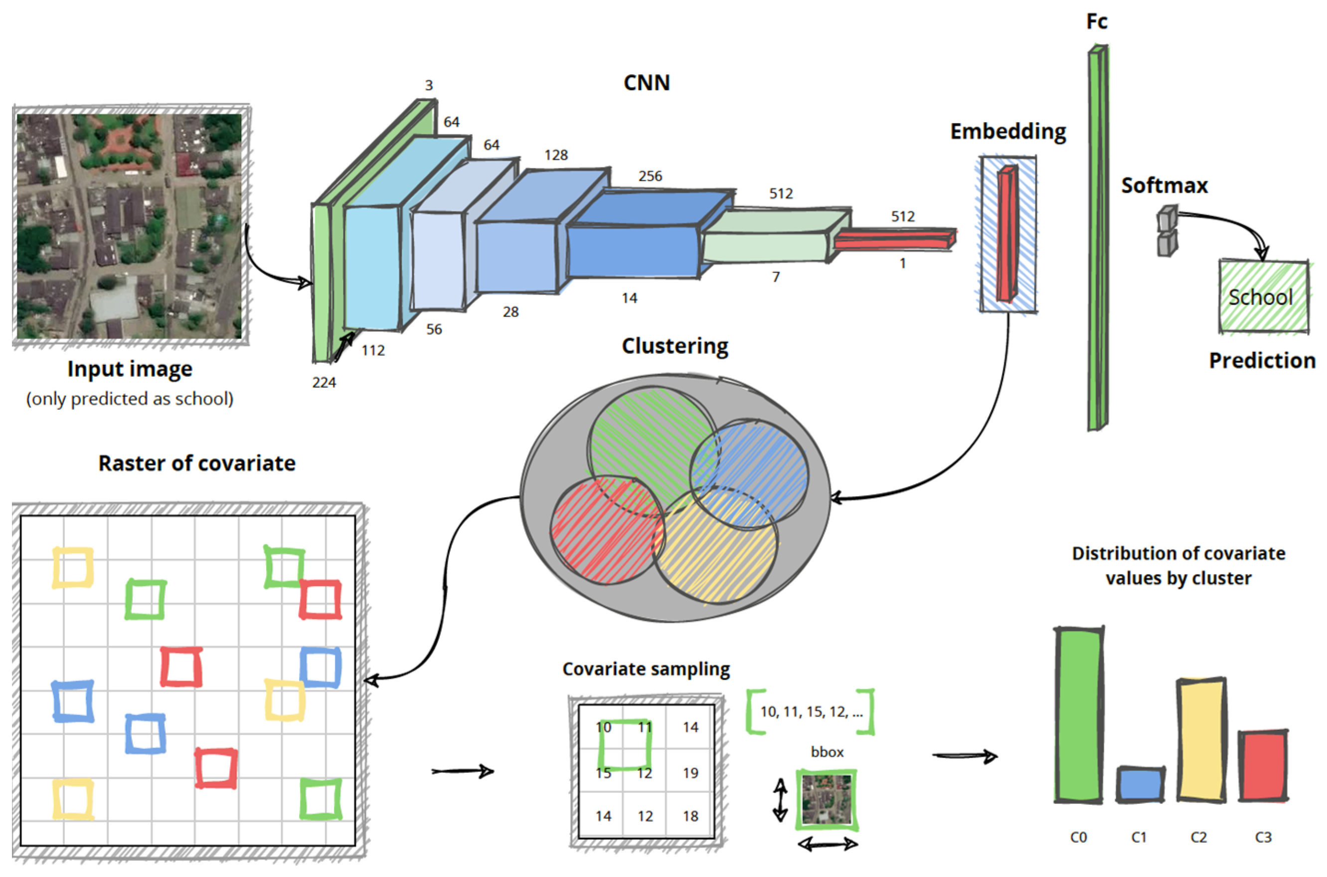
Among the different deep learning models that we tested, anti-aliased ResNet18 demonstrated the best accuracy overall. Table 1 shows the test results by different algorithms.

The anti-aliased ResNet18 model achieved an overall accuracy of 84%, which is relatively higher when compared to recent studies [50] and considering the complexity of the task and the simplicity of the approach. For the test set, the performance of the model was assessed, taking into account two possible labels “school” (236 images) and “not-school” (449 images). Figure 2 shows the learning curve of the anti-aliased ReseNet18 model.

The model accuracy for “school” labels was 0.84, and for images labeled “not-school”, it was 0.74. Analogously, we found that the precision was 0.74 and 0.91, respectively, the recall was 0.87 and 0.84, respectively, while the F₁-score was 0.79 and 0.87, respectively. The precision and F₁-scores for the “not-school” label were better than those for the “school” label, i.e., the classifier was more likely to fail when predicting the “school” label rather than the “not-school.”

Table 2. Confusion matrix of the classification results from anti-aliased ResNet18 model.

Truth\Prediction	School	Not School	Sum
School	200	36	236
Not-School	71	378	449
Sum	271	414	685

shows the confusion matrix between school and not-school samples.

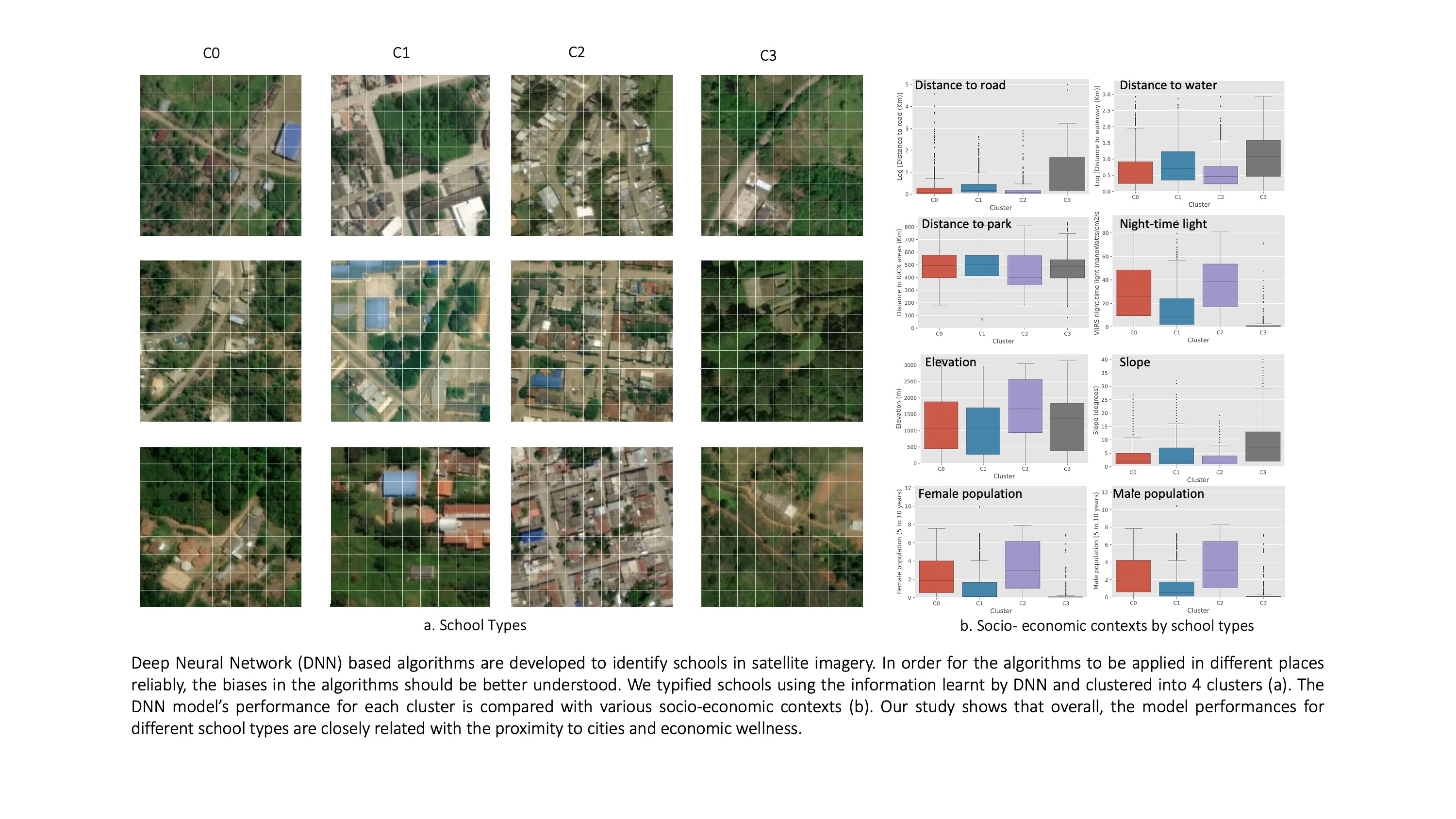
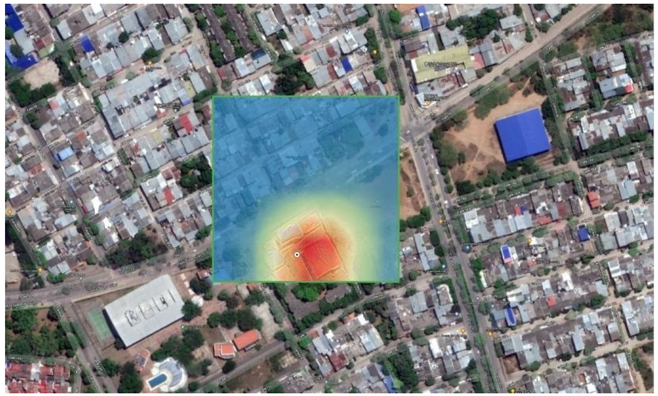
Even if the classifier correctly classifies an image as “school”, it is possible that what the neural network learned were some other characteristics common to all the samples in the dataset. To ensure that the classifier was actually detecting school buildings, we used Gradient-Weighted Class Activation Mapping (Grad-CAM), which showed where in the satellite image tile the model was looking at [51]. A visual explanation of what the model does is depicted in Figure 3 (each blue-yellow-red map to the right of the satellite image).

We found that nearly 83% of the model’s predictions located the correct building. The later analysis was performed manually, visually inspecting the regions obtained from the gradient class activation and comparing them against the ground truth (the real images with a dot on top of the school building). From the accuracy assessment and Grad-CAM, we confirmed that the model was correctly identifying the vast majority of school buildings.

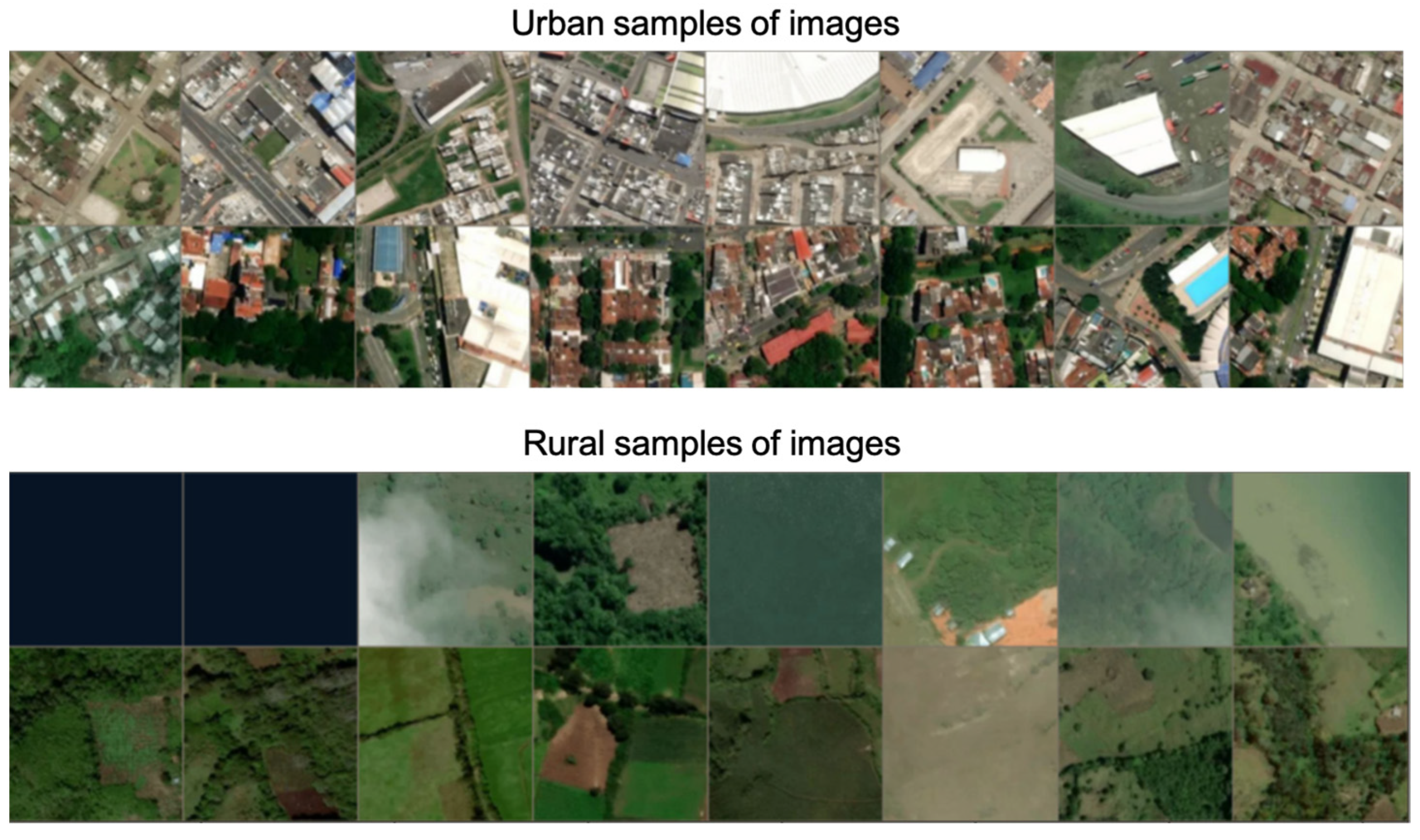
An assumption about our model was that it may work differently in different places. To test the assumption before a further analysis on different socioeconomic contexts, we summarized the result of the classification to show the differences in the accuracies between an urban area and rural area (

Table 3. Summary of the classification results by urban and rural areas.

Model	Acc.	Subset	Label	Precision	Recall	F1-Score	N
ResNet18 Anti-Aliased	0.696	Urban	school	0.720	0.853	0.781	163
			not_school	0.625	0.426	0.506	94
	0.932	Not-urban	school	0.782	0.836	0.808	73
			not_school	0.966	0.952	0.959	355

). For the distinction between urban and rural areas, we used the data and definition from the Global Human Settlement Layer [52]. From the comparison between the results for urban and rural areas, we found a very high difference in the model accuracies (diff: 0.236) between subsets. The model accuracy was better for the rural subset than the urban one. Further analysis of the confusion matrix for urban and rural areas revealed more detailed insights on the performance of our model (

Table 4. Confusion matrix of the classification results for urban and rural areas.

Urban Area
Truth\Prediction	School	Not School	Sum
School	139	24	163
Not-School	54	40	94
Sum	193	64	257
Rural Area
Truth\Prediction	School	Not School	Sum
School	56	17	73
Not-School	16	339	355
Sum	72	356	428

).

In urban areas, our model performed much less effectively when predicting the not-school class. This implies that in the urban class compared to school areas, the model was biased towards schools and making over-predictions. Contrarily, the model performed with very high accuracy (recall: 0.952, F₁-score: 0.959) for the not-school label in the rural subset. However, Figure 4 shows that there were many images without buildings in the rural subset, making it easy for the classifier to detect the lack of buildings as not-schools and produce higher accuracy metrics.

4.2. Clustering

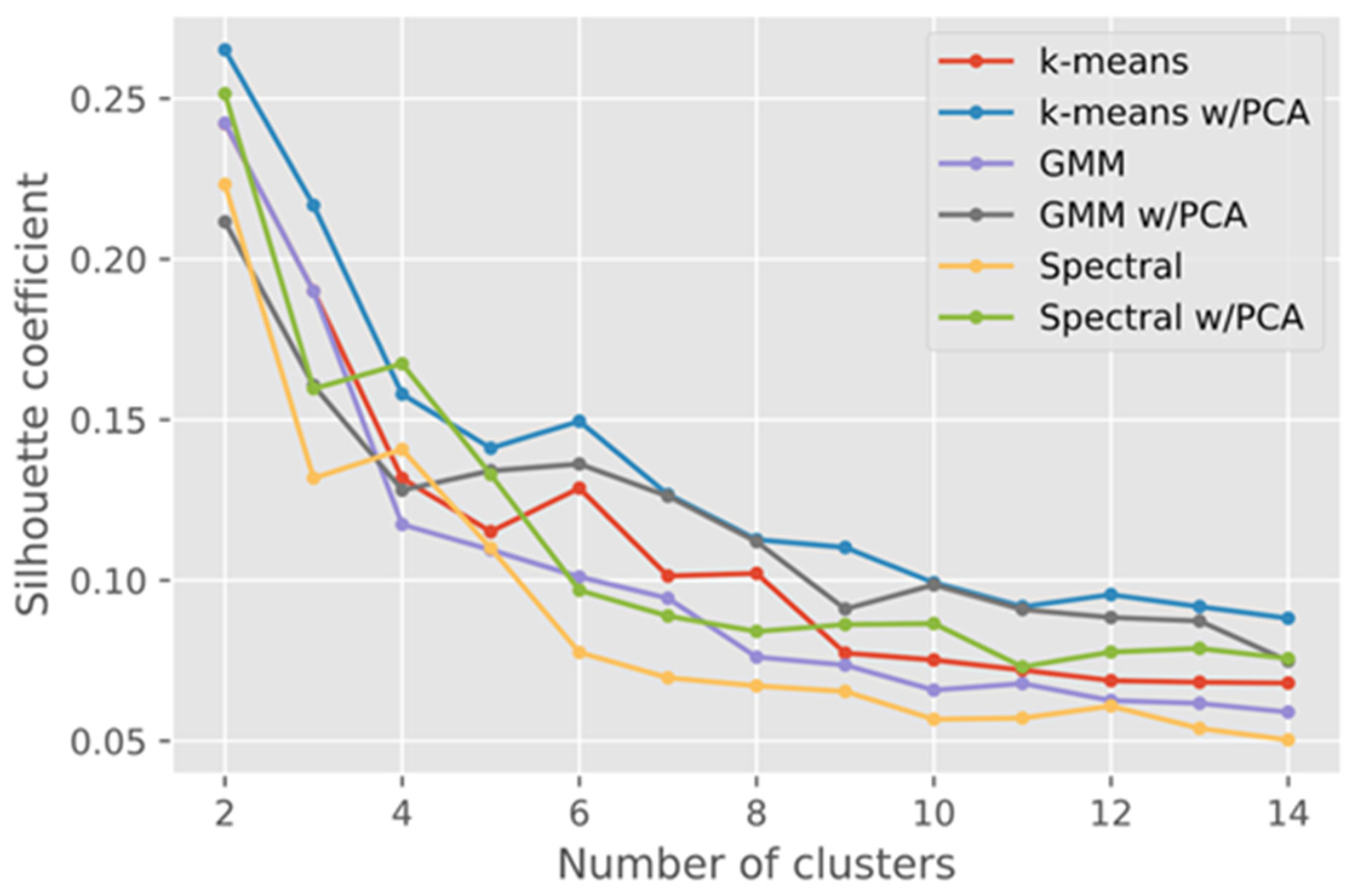
Having a model able to identify school buildings, we continued to identify sub-types of school images using clustering methods. We tested different clustering algorithms, different numbers of possible clusters and finally used the Silhouette Coefficient to evaluate the results obtained.

From Figure 5, we can observe that k-means with PCA dimensionality reduction gave the best results based on the Silhouette Coefficient [45]. The coefficients from different clustering methods with and without applying Principal Component Analysis (PCA) were comparatively low, which means a relatively high overlap between clusters [47]. Based on this observation, k-means with PCA was chosen as the method for clustering. Then, using the heuristic Elbow method [53], we obtained the optimal number of clusters of four. Figure 6 shows the number of clusters chosen using Elbow and Silhouette methods, with a visualization of clusters in two-dimensional space using T-distributed stochastic neighbor embedding (t-SNE).

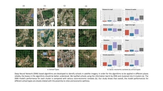
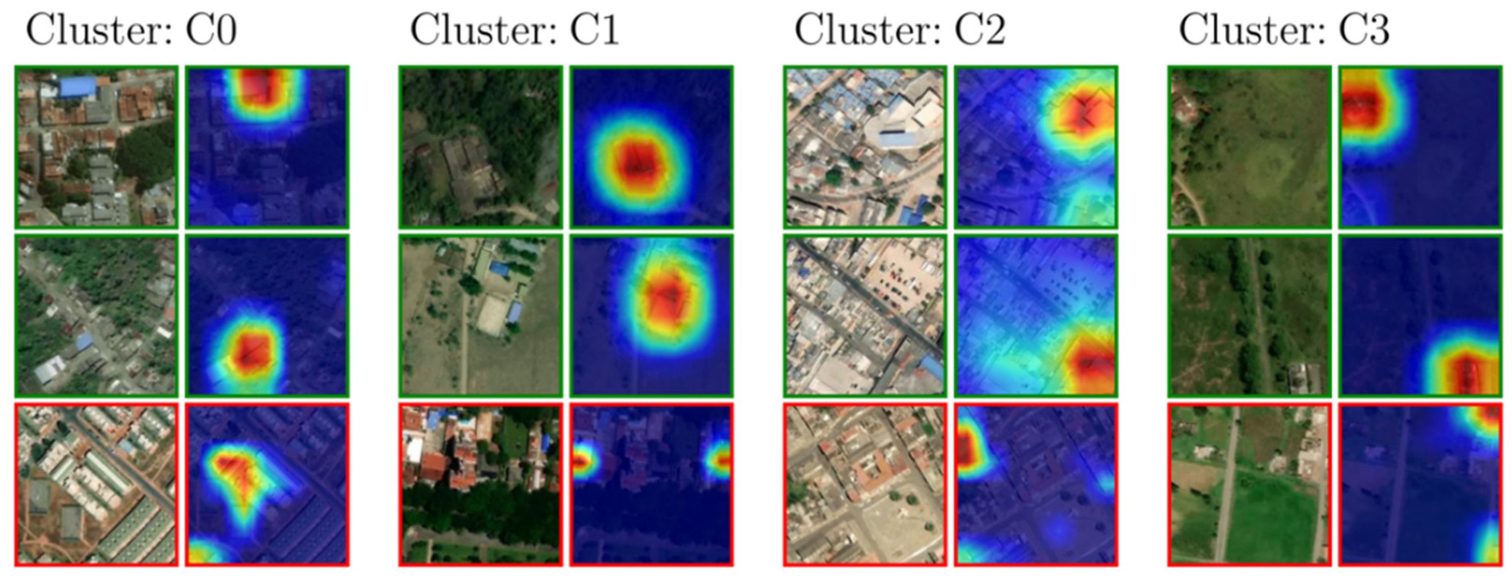
We labeled the four clusters with numbers ranging from 0 to 3: C0 (529 elements), C1 (273 elements), C2 (330 elements), and C3 (172 elements). We visually investigated each cluster for any noticeable patterns. From this, we concluded that clusters were largely decided by the characteristics of landscape (amount of vegetation, urban versus rural) in the area where the school buildings were located rather than by the features from the school buildings themselves.

In Figure 7, we can observe three images sampled for each cluster together with their respective Grad-CAM heatmap. The color of the border around each image indicates if a school was present or not in the image. Each group of four images corresponds to a cluster, with its corresponding label on top. From inspecting the images in each cluster, we can observe that cluster C2 was mostly urban, while cluster C3 was mostly rural. Clusters C0 and C1 had a larger diversity with mixed urban and rural images in them. The three images depicted for each cluster follow a specific logic. The two images on the top (with the green border) are the most representative images in each cluster that were at the same time true positives (contained a school building and were classified as schools). In this case, the most representative image was measured using the highest value of the Silhouette Coefficient. On the other hand, the picture in the bottom with the red border with the least representative image in the cluster was a false positive (it did not have a school but was classified as having one). The color of the border in Figure 7 indicates whether our classification algorithm correctly predicted a school or not. A green border represents an accurate prediction, while a red border indicates an incorrect one.

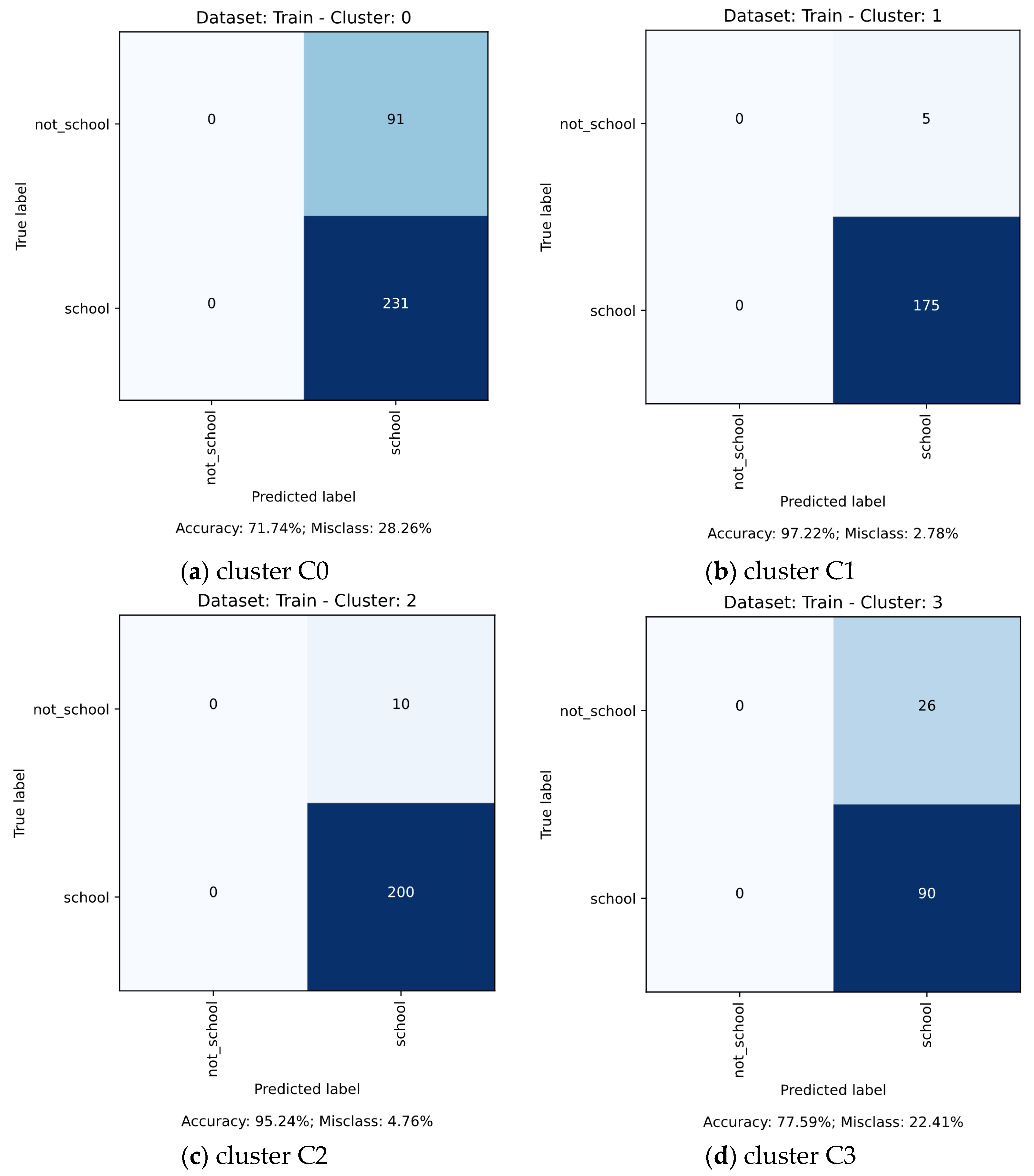
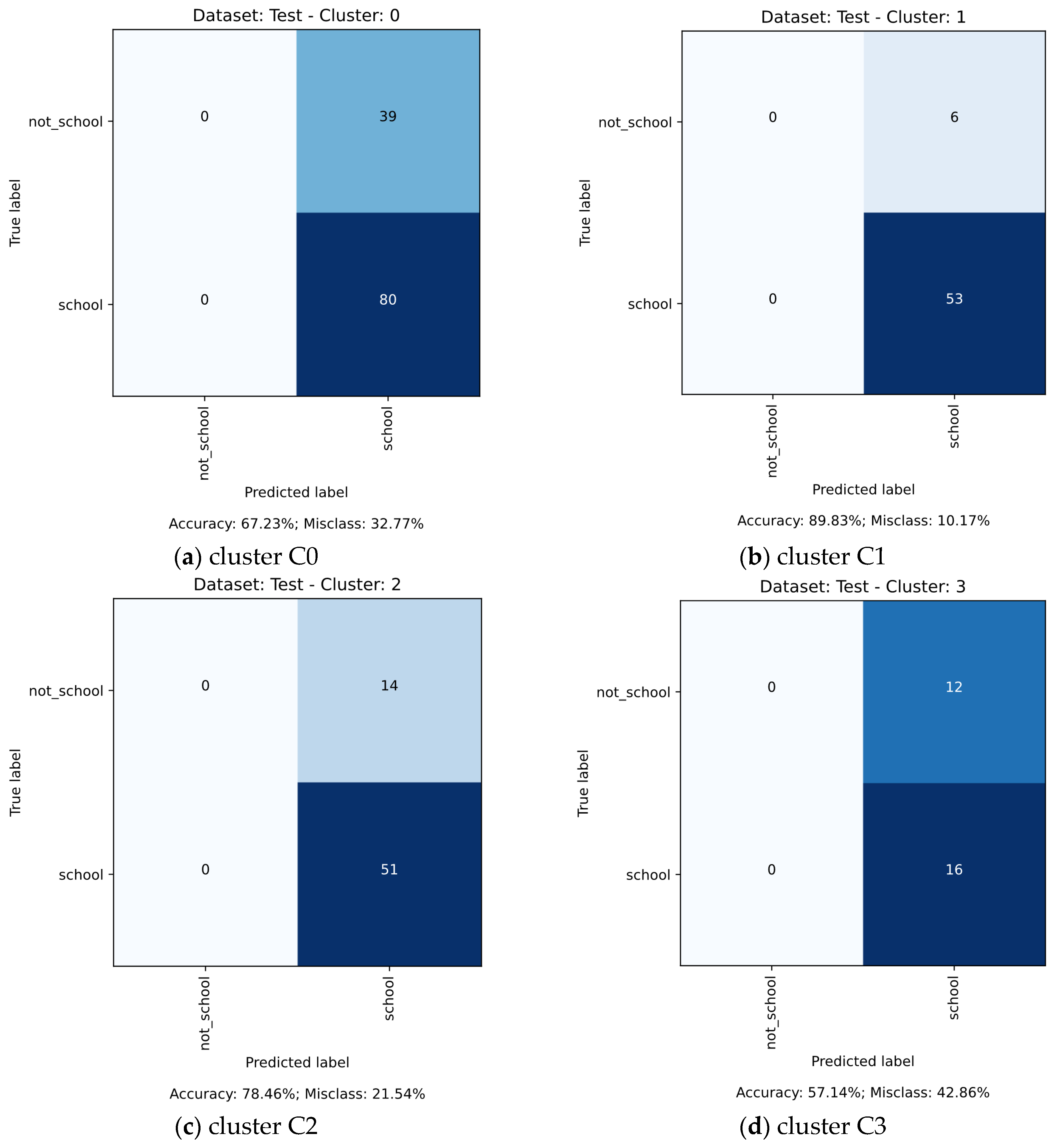
Having described the four clusters and their characteristics, we delved into the main question of the paper: is there an intrinsic bias in the model? To tackle this unknown, we studied the performance of the model per cluster instead of looking at the aggregate result.

Table 5. Training and testing accuracies obtained with the different clusters.

Dataset\Cluster	C0	C1	C2	C3
Train	0.717	0.972	0.952	0.776
Test	0.672	0.898	0.785	0.571

shows training and testing accuracies by each cluster. Clusters C0 and C3, which had characteristics of rural areas, showed a relatively lower test and train accuracy compared to clusters C1 and C2, which were mostly urban. The numbers presented above clearly show that the schools in the clusters with urban characteristics could be identified much better. The number of red and green borders in Figure 7 is not representative of the accuracy of each cluster. Those representatives were obtained by random sampling from each cluster. Since urban areas are typically wealthier than their rural counterparts, we tried to understand if the bias in the clusters was correlated to socioeconomic covariates and, therefore, if the model was negatively biased towards poorer communities.

4.3. Socioeconomic Covariates Analysis

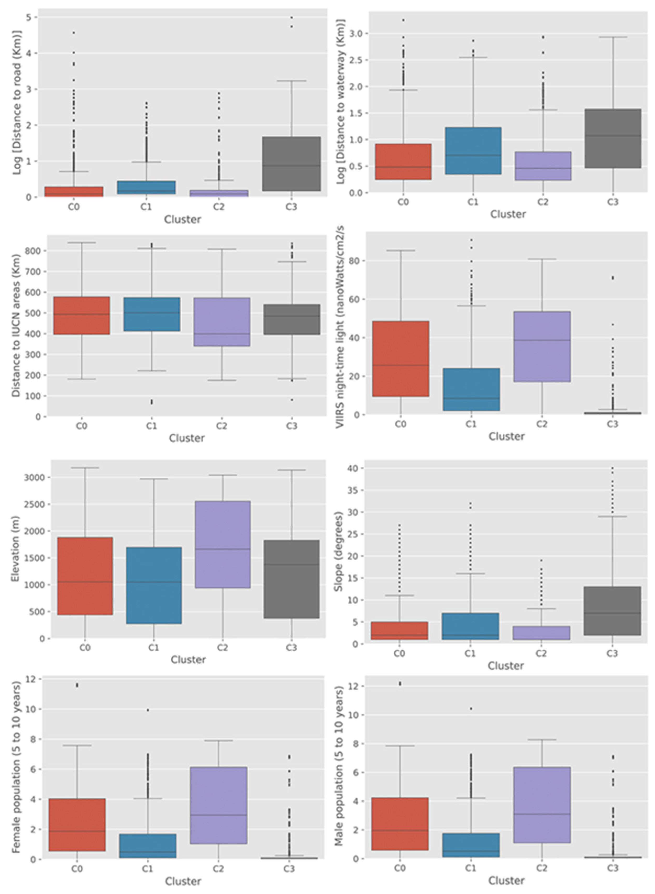
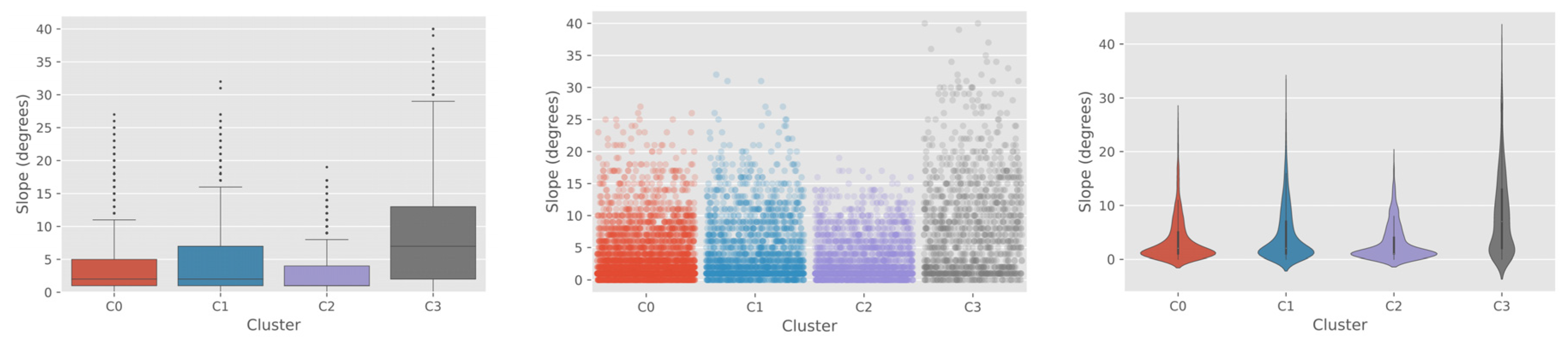
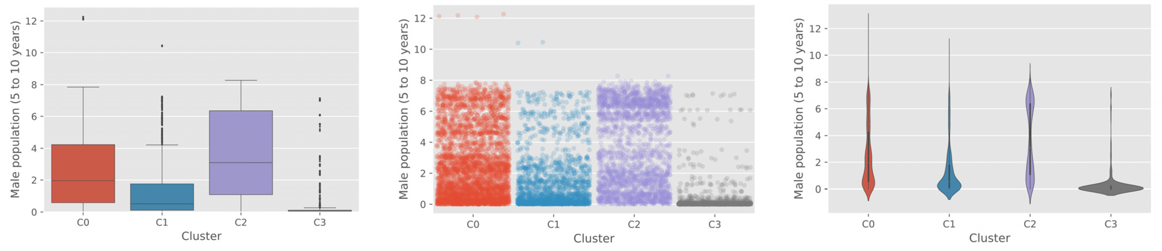
The distribution of various socioeconomic values within each cluster is presented in Figure 7. The most noticeable and clear findings from the socioeconomic covariate analysis was that cluster C3 was located in the most rural and remote regions with the lowest income level and the smallest child population, as shown in Figure 8.

The high slope values observed for cluster C3 also represent a characteristic of the impoverished areas in general [48]. We have identified that the accuracy of the deep learning model was lowest in the cluster C3 (0.78 and 0.57 for the train and test dataset, respectively), and these findings confirm our original assumption and previous studies [21,22,23] that DNN would be less effective in the context of landscape linked with vulnerability. More detailed accuracy matrices are shown in Figure A1 and Figure A2.

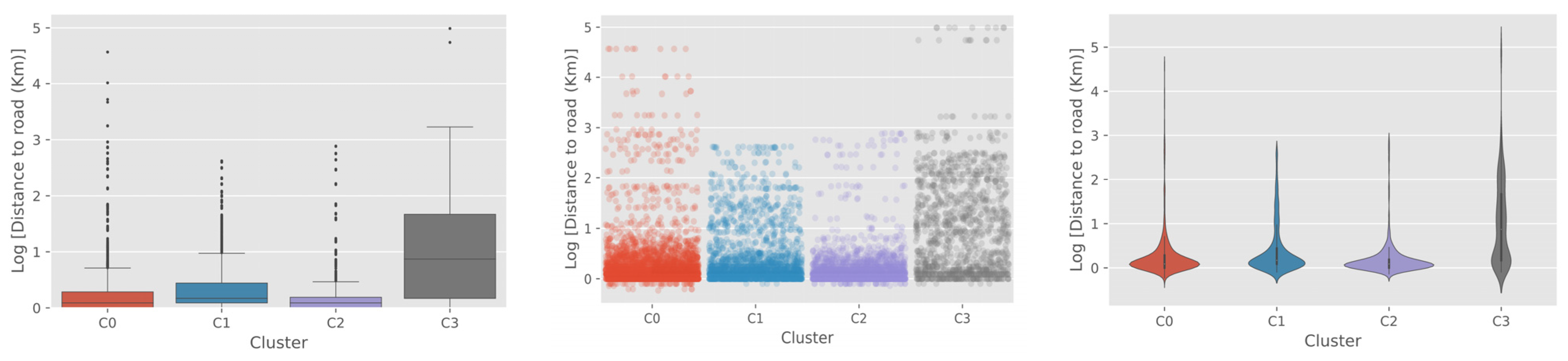
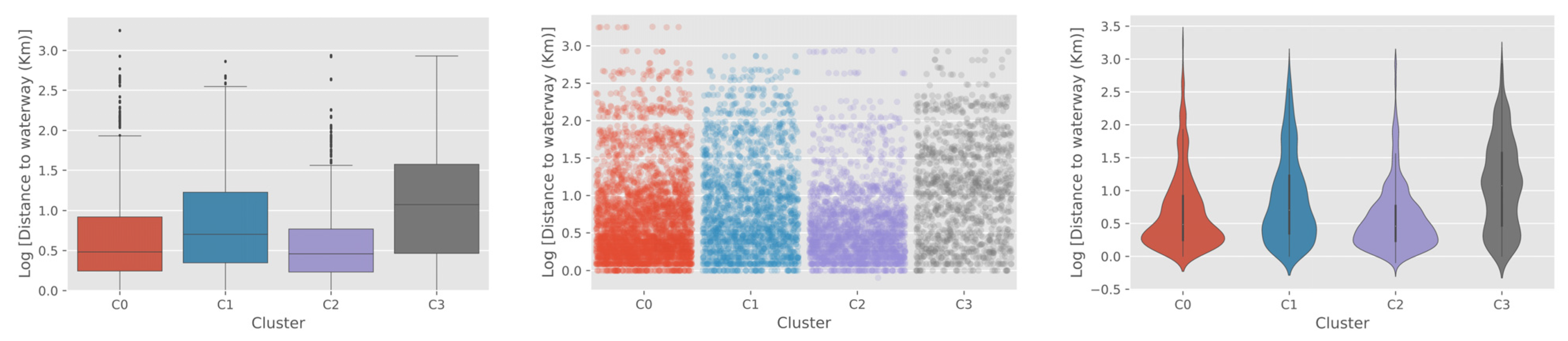
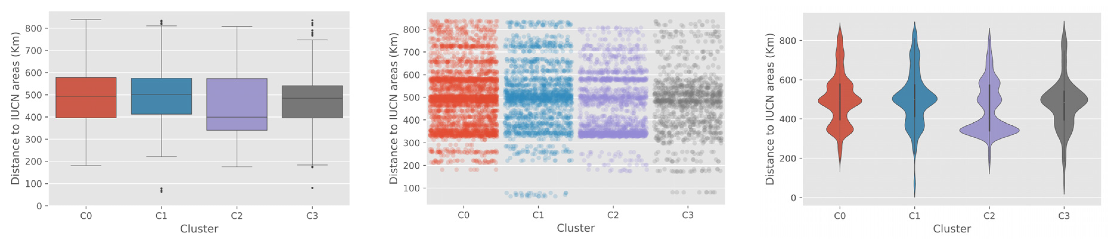
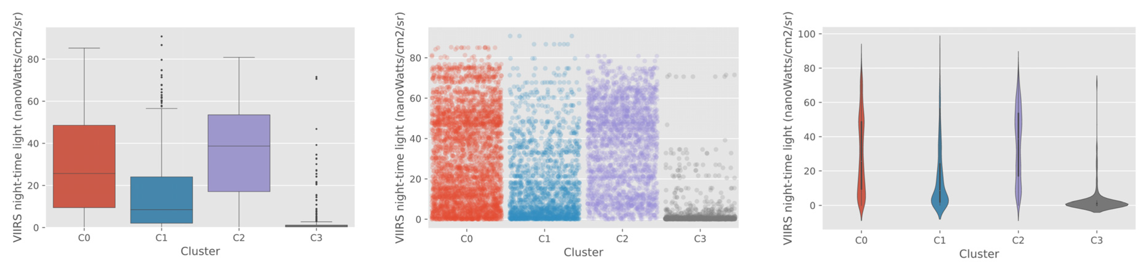
Figure 8 also reveals differences between clusters in multiple dimensions, which we could not recognize from a simple visual inspection using the natural color composite of optical remote sensing data. From the visual inspection using satellite imagery, C3 and C0 looked similar, both showing the typical characteristics of rural areas (Figure 7). However, when the two clusters were compared for the distribution of night-time light values, which is commonly used as a proxy for economic status [54], C0 showed a much wider distribution of values and a higher mean value compared to C3. This implies the income level in C0 would be comparatively higher than C3, which might have resulted in forming the physical characteristics of school buildings in the cluster. In terms of distance to road and water, C0 showed a similar distribution and mean values with the urban clusters C1 and C2. This reaffirms the difference between clusters C0 and C3, which might have caused the difference in model performance. 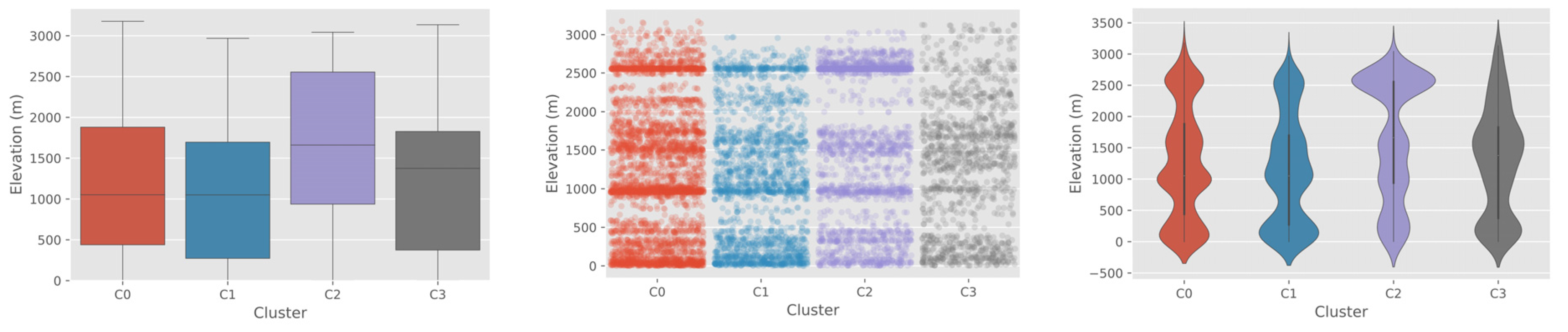In contrast, C1 and C2 showed higher accuracy and were linked with characteristics of well-developed and well-connected urban areas, as shown in Figure 8, which supports our original assumption. However, differences between those two clusters were also identified in the distributions of socioeconomic covariates. While C2 showed a typical characteristic of densely populated city area with the highest level of night-time light values, short distance to road and water, the largest child population, and the overall highest level of elevation [55], C1 showed the characteristics of sub-urban area with a proximity to infrastructures but with low population density. The slightly different model accuracy between C1 and C2 seems to have been driven by such a difference between the two clusters. More details on each socioeconomic variable can be found in Appendix B (Figure A3, Figure A4, Figure A5, Figure A6, Figure A7, Figure A8, Figure A9 and Figure A10).

In this study, we could typify schools in Colombia in different contexts using cluster analysis based on feature information extracted from a deep learning algorithm model trained from satellite imagery to identify school buildings. This allowed us to understand how the algorithm performed in heterogeneous socioeconomic contexts. While we could confirm our initial assumption that the model accuracy is lowest in the places where the most vulnerable populations are, there are some limitations that need to be addressed in future studies.

We clustered school image tiles into four clusters and later interpreted each as a type of school. However, the results of clustering seem widely based on the context of landscapes in which the schools were located, and we could not identify features directly from the school building itself. Urban, wealthy, and closely located schools were much better identified by DNN. This may be related to some quantifiable physical characteristics of school buildings, such as size, color, and material. In this study, we did not measure such attributes of school buildings directly. We envision that such variables about individual school buildings can be used to typify school buildings better.

Geospatial variables were selected considering their availability and relevance to the characteristics of the landscape, which we assumed would have been linked to the performance of the deep learning model. That is to say that socioeconomic covariates, which we assumed to be related to vulnerability and representativeness, such as poverty and child population, were selected and proved to have a strong relationship with the model’s performance. Nevertheless, we admit that the list of socioeconomic variables used in this study is far from inclusive from the list of all potential factors linked with the contexts of landscapes and land use characterization. Furthermore, we are aware of the potential measurement bias that arises from our choice of covariates as proxies. One difficulty in the process of covariate selection was that there is virtually no previous study that tried to prove the relationships between DNN’s performance to characterize land use and the socioeconomic context of landscapes where the subjects of the models are located. This study has benefited enormously from the socioeconomic geospatial dataset from WorldPop [39]. Such public repositories providing up-to-date and disaggregated geospatial datasets are essential for such an approach as taken by our study.

Retraining the model with a new, balanced dataset of tiles would be the next step to obtaining greater accuracy and minimizing bias. While we recommend our framework to assess biases and to make strategies to rectify them, it should be noted that sampling for a new training dataset based on an analysis of a limited number of covariates is not desirable before a comprehensive analysis of them. For example, one may normally expect that the values of a covariate most present in cluster C3 are those less represented in the dataset since it was the cluster with the worst accuracy (Figure 8). Nevertheless, this was not the case for the female and male child population and night-time light data (Figure 8). In fact, the low range values for those covariates, which were mostly seen in cluster C3, were well represented in the training dataset.

It is also worth mentioning that the DNN used in this study was fine-tuned and not trained from scratch. Since it is well known that some datasets used to pre-train these networks are biased (such as ImageNet [56]), some bias found can be due to the original bias in the pre-trained network, of which development was heavily concentrated on the developed world [18]. Given the case, it would be important to devise a procedure to understand and reduce the pre-existing biases before proceeding to train the model with one’s own data.

5. Conclusions

At the beginning of this article, we argued that because of the lack of explainability and biases in the DNN base model for land use classification, it would demonstrate worse efficacy for the most vulnerable communities. Explainability is one of the most crucial factors of AI algorithms if they are to be applied to real-world problems, but unfortunately, not many advances have been seen in the field of LULCC, especially for the applications on land use classification. Through a novel combination of techniques ranging from DNN to clustering algorithms, we explored and identified biases in AI, rendering the process of automatic identification of schools more transparent and explainable.

Through our study, we identified three possible sources of bias in the DNN base models: the socioeconomic covariates used as a proxy for socioeconomic development, the bias from the sample of images used to train the model, and the bias introduced by the original dataset used to pre-train our deep neural network. One of the most critical findings from this study is that DNN based models could be least effective for the most vulnerable communities. This finding is important when the DNN based results are used in a project to solve real-world issues because such biases in DNN models can significantly undermine the effectiveness of development projects which are increasingly dependent on data and insights produced using DNN. As such, we envision that the framework of our study could be applied to enlighten the errors and biases in DNN based models adopted in various types of humanitarian operations.

We have identified some lines of future work that could improve the bias detection framework presented in this paper. First, we may increase the number of clusters with more training samples to detect the more nuanced differences from the school buildings. Second, another approach worth considering would be to extract the identified school from each image (using the class activation gradient) and then train a new model with less noise only on the most important section of the image: the building itself. Furthermore, an ensemble model [57] could be used to take both kinds of features: the type of buildings and the landscape that surrounds them. It would also be fruitful to pursue further research about the relationship between a Deep Neural Network’s performance and the socioeconomic context of the landscapes where the subjects of the models are located, aiming to discover more geospatial variables linked with the performance of the model.

Finally, we hope that our study contributes to enhancing the awareness of the importance of the explainable and equitable algorithms for the development sector.

References

1. Lecun, Y.; Bengio, Y.; Hinton, G. Deep learning. Nature 2015, 521, 436–444. [Google Scholar] [CrossRef]
2. Scott, G.J.; England, M.R.; Starms, W.A.; Marcum, R.A.; Davis, C.H. Training deep convolutional neural networks for land-cover classification of high-resolution imagery. IEEE Geosci. Remote Sens. Lett. 2017, 14, 549–553. [Google Scholar] [CrossRef]
3. Helber, P.; Bischke, B.; Dengel, A.; Borth, D. Eurosat: A novel dataset and deep learning benchmark for land use and land cover classification. IEEE J. Sel. Top. Appl. Earth Obs. Remote Sens. 2019, 12, 2217–2226. [Google Scholar] [CrossRef] [Green Version]
4. Kussul, N.; Shelestov, A.; Lavreniuk, M.; Butko, I.; Skakun, S. Deep Learning Approach for Large Scale Land Cover Mapping Based on Remote Sensing Data Fusion. In Proceedings of the 2016 IEEE International Geoscience and Remote Sensing Symposium (IGARSS), Beijing, China, 10–15 July 2016; pp. 198–201. [Google Scholar]
5. Srivastava, S.; Vargas-Munoz, J.E.; Tuia, D. Understanding urban landuse from the above and ground perspectives: A deep learning, multimodal solution. Remote Sens. Environ. 2019, 228, 129–143. [Google Scholar] [CrossRef] [Green Version]
6. Ma, L.; Liu, Y.; Zhang, X.; Ye, Y.; Yin, G.; Johnson, B.A. Deep learning in remote sensing applications: A meta-analysis and review. ISPRS J. Photogramm. Remote Sens. 2019, 152, 166–177. [Google Scholar] [CrossRef]
7. Di Gregorio, A. Land Cover Classification System: Classification Concepts and User Manual: LCCS.; Food and Agriculture Organization of the United Nations: Rome, Italy, 2005; Volume 2. [Google Scholar]
8. Vinet, L.; Zhedanov, A. A “missing” family of classical orthogonal polynomials. J. Phys. A Math. Theoretical. 2011, 44, 21–25. [Google Scholar] [CrossRef]
9. Tiecke, T.G.; Liu, X.; Zhang, A.; Gros, A.; Li, N.; Yetman, G.; Kilic, T.; Murray, S.; Blankespoor, B.; Prydz, E.B.; et al. Mapping the world population one building at a time. arXiv 2017, arXiv:1712.05839. [Google Scholar]
10. Cao, R.; Tu, W.; Yang, C.; Li, Q.; Liu, J.; Zhu, J.; Zhang, Q.; Li, Q.; Qiu, G. Deep learning-based remote and social sensing data fusion for urban region function recognition. ISPRS J. Photogramm. Remote Sens. 2020, 163, 82–97. [Google Scholar] [CrossRef]
11. Lang, S.; Füreder, P.; Riedler, B.; Wendt, L.; Braun, A.; Tiede, D.; Schoepfer, E.; Zeil, P.; Sprohnle, K.; Lulessa, K. Earth observation tools and services to increase the effectiveness of humanitarian assistance. Eur. J. Remote Sens. 2020, 53 (Suppl. S2), 67–85. [Google Scholar] [CrossRef] [Green Version]
12. ITU and UNICEF Have Joined Forces to Connect Every School to the Internet. Available online: https://www.itu.int/en/ITU-D/Initiatives/GIGA/Pages/default.aspx (accessed on 21 July 2021).
13. Yi, Z.; Zurutuza, N.; Bollinger, D.; Garcia-Herranz, M.; Kim, D. Towards equitable access to information and opportunity for all: Mapping schools with high-resolution Satellite Imagery and Machine Learning. In Proceedings of the IEEE Conference on Computer Vision and Pattern Recognition Workshops, Long Beach, CA, USA, 16–20 June 2019; pp. 60–66. [Google Scholar]
14. Kleinberg, J.; Ludwig, J.; Mullainathan, S.; Sunstein, C.R. Algorithms as discrimination detectors. Proc. Natl. Acad. Sci. USA 2020, 117, 30096–30100. [Google Scholar] [CrossRef]
15. Sweeney, L. Discrimination in online ad delivery. Commun. ACM 2013, 56, 44–54. [Google Scholar] [CrossRef]
16. Barocas, S.; Selbst, A.D. Big data’s disparate impact. Calif. L. Rev. 2016, 104, 671. [Google Scholar] [CrossRef]
17. Bornstein, S. Antidiscriminatory algorithms. Ala. L. Rev. 2018, 70, 519. [Google Scholar]
18. Andersen, L. Artificial Intelligence in International Development: Avoiding Ethical Pitfalls. Available online: https://jpia.princeton.edu/news/artificial-intelligence-international-development-avoiding-ethical-pitfalls (accessed on 21 July 2021).
19. Mehrabi, N.; Morstatter, F.; Saxena, N.; Lerman, K.; Galstyan, A. A survey on bias and fairness in machine learning. arXiv 2019, arXiv:1908.09635. [Google Scholar]
20. Luengo-Oroz, M.; Bullock, J.; Pham, K.H.; Lam, C.S.N.; Luccioni, A. From Artificial Intelligence Bias to Inequality in the Time of COVID-19. IEEE Technol. Soc. Mag. 2021, 40, 71–79. [Google Scholar] [CrossRef]
21. Hutchinson, B.; Prabhakaran, V.; Denton, E.; Webster, K.; Zhong, Y.; Denuyl, S. Unintended machine learning biases as social barriers for persons with disabilitiess. ACM SIGACCESS Access. Comput. 2020, 125, 1. [Google Scholar] [CrossRef] [Green Version]
22. Cirillo, D.; Catuara-Solarz, S.; Morey, C.; Guney, E.; Subirats, L.; Mellino, S.; Gigante, A.; Valencia, A.; Rementeria, M.J.; Chadha, A.S.; et al. Sex and gender differences and biases in artificial intelligence for biomedicine and healthcare. NPJ Digit. Med. 2020, 3, 1–11. [Google Scholar] [CrossRef] [PubMed]
23. Shankar, S.; Halpern, Y.; Breck, E.; Atwood, J.; Wilson, J.; Sculley, D. No classification without representation: Assessing geodiversity issues in open data sets for the developing world. arXiv 2017, arXiv:1711.08536. [Google Scholar]
24. Aubakirova, M.; Bansal, M. Interpreting neural networks to improve politeness comprehension. arXiv 2016, arXiv:1610.02683. [Google Scholar]
25. Liu, N.; Huang, X.; Li, J.; Hu, X. On interpretation of network embedding via taxonomy induction. In Proceedings of the 24th ACM SIGKDD International Conference on Knowledge Discovery & Data Mining, London, UK, 19–23 August 2018; pp. 1812–1820. [Google Scholar]
26. Chollet, F. Deep Learning with Python; Simon and Schuster: New York, NY, USA, 2017. [Google Scholar]
27. CS231n: Convolutional Neural Networks for Visual Recognition. Available online: http://cs231n.stanford.edu (accessed on 21 July 2021).
28. Krizhevsky, A.; Sutskever, I.; Hinton, G.E. Imagenet classification with deep convolutional neural networks. Adv. Neural Inf. Process. Syst. 2021, 25, 1097–1105. [Google Scholar] [CrossRef]
29. Simonyan, K.; Zisserman, A. Very deep convolutional networks for large-scale image recognition. In Proceedings of the 3rd International Conference on Learning Representations, ICLR 2015—Conference Track Proceedings (1–14), San Diego, CA, USA, 7–9 May 2015. [Google Scholar]
30. Yun, J.W. Deep Residual Learning for Image Recognition. Enzym. Microb. Technol. 2015, 19, 107–117. [Google Scholar] [CrossRef]
31. Imagenet: Vggnet, Resnet, Inception, and Xception with Keras. Available online: https://www.pyimagesearch.com/2017/03/20/imagenet-vggnet-resnet-inception-xception-keras/ (accessed on 21 July 2021).
32. Howard, A.G.; Zhu, M.; Chen, B.; Kalenichenko, D.; Wang, W.; Weyand, T.; Andreetto, M.; Adam, H. Mobilenets: Efficient convolutional neural networks for mobile vision applications. arXiv 2017, arXiv:1704.04861. [Google Scholar]
33. Ren, S.; He, K.; Girshick, R.; Sun, J. Faster r-cnn: Towards real-time object detection with region proposal networks. Adv. Neural Inf. Process. Syst. 2015, 28, 91–99. [Google Scholar] [CrossRef] [Green Version]
34. Dai, J.; Li, Y.; He, K.; Sun, J. R-fcn: Object detection via region-based fully convolutional networks. arXiv 2016, arXiv:1605.06409v. [Google Scholar]
35. Redmon, J.; Divvala, S.; Girshick, R.; Farhadi, A. You only look once: Unified, real-time object detection. In Proceedings of the IEEE Conference on Computer Vision and Pattern Recognition, Las Vegas, NV, USA, 26 July 2016; pp. 779–788. [Google Scholar]
36. Liu, W.; Anguelov, D.; Erhan, D.; Szegedy, C.; Reed, S.; Fu, C.-Y.; Berg, A.C. SSD: Single Shot MultiBox Detector. arXiv 2015, arXiv:1512.02325. [Google Scholar]
37. O’Shea, K.; Nash, R. An introduction to convolutional neural networks. arXiv 2015, arXiv:1511.08458. [Google Scholar]
38. A Comprehensive Guide to Convolutional Neural Networks—The ELI5 Way. Available online: https://towardsdatascience.com/a-comprehensive-guide-to-convolutional-neural-networks-the-eli5-way-3bd2b1164a53 (accessed on 23 July 2021).
39. Lloyd, C.T.; Chamberlain, H.; Kerr, D.; Yetman, G.; Pistolesi, L.; Stevens, F.R.; Gaughan, A.E.; Nieves, J.J.; Hornby, G.; MacManus, K.; et al. Global spatio-temporally harmonised datasets for producing high-resolution gridded population distribution datasets. Big Earth Data 2019, 3, 108–139. [Google Scholar] [CrossRef] [PubMed] [Green Version]
40. Zhang, R. Making convolutional networks shift-invariant again. In Proceedings of the International Conference on Machine Learning, Long Beach, CA, USA, 10 June 2019; pp. 7324–7334. [Google Scholar]
41. Paszke, A.; Gross, S.; Massa, F.; Lerer, A.; Bradbury, J.; Chanan, G.; Killeen, T.; Lin, Z.; Gimelshein, N.; Antiga, L.; et al. Pytorch: An imperative style, high-performance deep learning library. arXiv 2019, arXiv:1912.01703. [Google Scholar]
42. Ng, A.Y.; Jordan, M.I.; Weiss, Y. On spectral clustering: Analysis and an algorithm. Adv. Neural Inf. Process. Syst. 2002, 2, 849–856. [Google Scholar]
43. Reynolds, D.A. Gaussian Mixture Models. Encycl. Biom. 2009, 741, 659–663. [Google Scholar]
44. Wold, S.; Esbensen, K.; Geladi, P. Principal component analysis. Chemom. Intell. Lab. Syst. 1987, 2, 37–52. [Google Scholar] [CrossRef]
45. Zhou, H.B.; Gao, J.T. Automatic method for determining cluster number based on silhouette coefficient. Adv. Mater. Res. 2014, 951, 227–230. [Google Scholar] [CrossRef]
46. Sakamoto, Y.; Ishiguro, M.; Kitagawa, G. Akaike information criterion statistics. Dordr. Neth. D Reidel 1986, 81, 26853. [Google Scholar]
47. Shahapure, K.R.; Nicholas, C. Cluster Quality Analysis Using Silhouette Score. In Proceedings of the 2020 IEEE 7th International Conference on Data Science and Advanced Analytics (DSAA), Sydney, Australia, 6 October 2020; pp. 747–748. [Google Scholar]
48. Agudelo, C.; Rivera, B.; Tapasco, J.; Estrada, R. Designing Policies to Reduce Rural Poverty and Environmental Degradation in a Hillside Zone of the Colombian Andes. World Dev. 2003, 31, 1921–1931. [Google Scholar] [CrossRef]
49. Foody, G.M. Status of land cover classification accuracy assessment. Remote Sens. Environ. 2002, 80, 185–201. [Google Scholar] [CrossRef]
50. Zhang, C.; Harrison, P.A.; Pan, X.; Li, H.; Sargent, I.; Atkinson, P.M. Scale Sequence Joint Deep Learning (SS-JDL) for land use and land cover classification. Remote Sens. Environ. 2020, 237, 111593. [Google Scholar] [CrossRef]
51. Selvaraju, R.R.; Cogswell, M.; Das, A.; Vedantam, R.; Parikh, D.; Batra, D. Grad-cam: Visual explanations from deep networks via gradient-based localization. In Proceedings of the IEEE International Conference on Computer Vision, Seattle, WA, USA, 14 June 2020; pp. 618–626. [Google Scholar]
52. Pesaresi, M.; Ehrilch, D.; Florczyk, A.J.; Freire, S.; Julea, A.; Kemper, T.; Soille, P.; Syrris, V. GHS Built-Up Grid, Derived from Landsat, Multitemporal (1975, 1990, 2000, 2014); JRC Data Catalogue; European Commission, Joint Research Centre: Brussels, Belgium, 2015. [Google Scholar]
53. Thorndike, R.L. Who belongs in the family? Psychometrika 1953, 18, 267–276. [Google Scholar] [CrossRef]
54. Doll, C.N.H.; Muller, J.-P.; Morley, J.G. Mapping regional economic activity from night-time light satellite imagery. Ecol. Econ. 2006, 57, 75–92. [Google Scholar] [CrossRef]
55. Engstrom, R.; Pavelesku, D.; Tanaka, T.; Wambile, A. Mapping Poverty and Slums Using Multiple Methodologies in Accra, Ghana. In Proceedings of the 2019 Joint Urban Remote Sensing Event (JURSE), Vannes, France, 22 May 2019; pp. 1–4. [Google Scholar]
56. Geirhos, R.; Rubisch, P.; Michaelis, C.; Bethge, M.; Wichmann, F.A.; Brendel, W. ImageNet-trained CNNs are biased towards texture; increasing shape bias improves accuracy and robustness. arXiv 2018, arXiv:1811.12231. [Google Scholar]
57. Sagi, O.; Rokach, L. Ensemble Learning: A Survey. Wiley Interdiscip. Rev. Data Min. Knowl. Discov. 2018, 8, e1249. [Google Scholar] [CrossRef]
Figure 1. Framework to assess biases in DNN based algorithms to map school locations from satellite imagery used in this study.
Remotesensing 13 02908 g001
Figure 2. Accuracy and loss graph of the anti-aliased ResNet18 model.
Remotesensing 13 02908 g002
Figure 3. Gradient class activation heatmap of the trained convolutional neural network over a “school” labeled satellite image tile. The point shows the school’s real location while the red color shows where the model looked in the image to predict “school”.
Remotesensing 13 02908 g003
Figure 4. Random sample of images on the test dataset by urban and rural subsets.
Remotesensing 13 02908 g004
Figure 5. Silhouette coefficient comparison profiles between different clustering algorithms with and without dimensionality reduction using PCA.
Remotesensing 13 02908 g005
Figure 6. Top left: finding the number of components based on the point of maximum curvature from the Principal Component Analysis. Top right: using the Elbow method to determine the k number of clusters. Bottom left: Silhouette Coefficients. Bottom right: two-dimensional color visualization of the CNN feature embedding after t-SNE, clustered according to the k-means algorithm.
Remotesensing 13 02908 g006
Figure 7. Images samples of each cluster and Gradient-Weighted Class Activation Mapping heatmaps.
Remotesensing 13 02908 g007
Figure 8. Distribution of socioeconomic variables within clusters.
Remotesensing 13 02908 g008