
The Key Reason of False Positive Misclassification for Accurate Large-Area Mangrove Classifications


1
Key Laboratory of Wetland Ecology and Environment, Northeast Institute of Geography and Agroecology, Chinese Academy of Sciences, Changchun 130102, China
2
State Key Laboratory of Resources & Environmental Information System, Institute of Geographical Sciences and Natural Resources Research, Chinese Academy of Sciences, Beijing 100101, China
3
College of Resources and Environment, University of Chinese Academy of Sciences, Beijing 100049, China
4
Jiangsu Center for Collaborative Innovation in Geographical Information Resource Development and Application, Nanjing 210023, China
*
Author to whom correspondence should be addressed.
Remote Sens. 2021, 13(15), 2909; https://0-doi-org.brum.beds.ac.uk/10.3390/rs13152909
Submission received: 14 June 2021
/
Revised: 13 July 2021
/
Accepted: 21 July 2021
/
Published: 24 July 2021
(This article belongs to the Special Issue GIS and RS in Ocean, Island and Coastal Zone)
Abstract
:Accurate large-area mangrove classification is a challenging task due to the complexity of mangroves, such as abundant species within the mangrove category, and various appearances resulting from a large latitudinal span and varied habitats. Existing studies have improved mangrove classifications by introducing time series images, constructing new indices sensitive to mangroves, and correcting classifications by empirical constraints and visual inspections. However, false positive misclassifications are still prevalent in current classification results before corrections, and the key reason for false positive misclassification in large-area mangrove classifications is unknown. To address this knowledge gap, a hypothesis that an inadequate classification scheme (i.e., the choice of categories) is the key reason for such false positive misclassification is proposed in this paper. To validate this hypothesis, new categories considering non-mangrove vegetation near water (i.e., within one pixel from water bodies) were introduced, which is inclined to be misclassified as mangroves, into a normally-used standard classification scheme, so as to form a new scheme. In controlled conditions, two experiments were conducted. The first experiment using the same total features to derive direct mangrove classification results in China for the year 2018 on the Google Earth Engine with the standard scheme and the new scheme respectively. The second experiment used the optimal features to balance the probability of a selected feature to be effective for the scheme. A comparison shows that the inclusion of the new categories reduced the false positive pixels with a rate of 71.3% in the first experiment, and a rate of 66.3% in the second experiment. Local characteristics of false positive pixels within 1 × 1 km cells, and direct classification results in two selected subset areas were also analyzed for quantitative and qualitative validation. All the validation results from the two experiments support the finding that the hypothesis is true. The validated hypothesis can be easily applied to other studies to alleviate the prevalence of false positive misclassifications.
1. Introduction
Mangroves are a community of trees and shrubs adapted to tidal environments found in tropical and subtropical regions of the world [1,2]. Mangroves provide a wide range of ecosystem services such as coast protection and carbon sinks, as well as materials such as food and medicine [3,4,5,6,7]. Mangroves distribution is dynamic as a result of deforestation for agriculture, aquaculture, and urban expansion [8,9,10] or afforestation efforts [11,12]. Remote sensing (RS)-based approaches have been developed to efficiently map mangrove distribution over large areas, especially since Giri, et al. [13] obtained a global mangrove distribution map using Landsat data. However, due to the presence of different mangrove species, a large latitudinal span, and the mixing with other forest types at the fringes, accurate large-area mangrove mapping remains a challenging task [14,15,16].
Existing RS-based studies on large-area mangrove classifications firstly derived mangroves by a classification procedure, and then corrected the classification results using various empirical constraints and visual inspections (i.e., post-processing) to obtain mangrove maps. Due to the widespread occurrence of false positive patches in direct classifications [17,18], the correction on the false positive misclassification is crucial. During the correction, the false positive misclassifications can be comparatively corrected by both empirical constraints and visual inspections, which highly rely on human experience. For example, distances have been widely used in mangrove mapping, such as the distance to coastline to screen out areas far away from coasts (e.g., 10 km by Hu, et al. [19]), and the distance to water to screen out false positive patches (e.g., 2.5 km by Xia, et al. [20]), which are still arbitrary for the large-area situation. Moreover, false positive misclassifications close to mangroves can easily escape from these constraints (e.g., the distance to coastline, the distance to water, and elevation). Thus, it is highly valuable to improve the performance of the classification procedure to obtain accurate large-area mangrove mapping.
In the classification procedure, the classification algorithms varied in forms [21,22,23], while containing the same core, that is, using samples to determine a decision surface [24,25,26,27] for optimally distinguishing the interest categories.
To improve the performance of mangrove classifications, the features of a sample have been augmented by introducing multi-temporal and/or multi-source images. Recent studies on mangrove classification have focused on the application of time series imagery [14,18,19,28]. However, Zhao and Qin [18] revealed widespread false positives that misclassified vegetation near water as mangroves, even though the increase of the samples’ features was adopted.
When the increase of features did not improve false positive misclassification much, the performance of mangrove classifications is affected by the adopted classification scheme (the classification scheme in this study is defined as the choice of categories) which determines the class diversity of samples and consequently affects the construction of the decision surface in partitioning the feature space according to samples’ membership in different classes [27,29]. However, there are few studies involved in the effects from classification schemes, and most of them designed classification schemes for standardization of classification results [30] rather than exploring a way to improve the classification results. Baloloy, et al. [31] applied a scheme of seven classes (i.e., mangroves, terrestrial vegetation (forest), terrestrial vegetation (non-forest), bare soil, built-up, water, and clouds) to determine the threshold for identifying mangroves, and Zhao and Qin [18] utilized a scheme of 10 classes (i.e., mangroves, coastal forests, salt marsh, grass, cropland, sand or rock, terrestrial forests, permanent water, tidal flats, and artificial impervious surfaces) to train a classifier for mangrove classification. These classification schemes do not well consider the uniqueness of coastal areas, which are affected by terrestrial and marine environments and anthropogenic activities [32,33]. A typical example is the widespread existence of aquaculture ponds [34], which are shown as small water bodies with vegetation strips on the edges. The non-mangrove vegetation strips near water bodies can be easily misclassified as mangroves [12,14,18,19]. Such land cover near water bodies does not belong to standard a priori classification schemes.
Therefore, in this study a hypothesis was proposed, that is, the inadequate consideration of non-mangrove vegetation near water in priori classification schemes is the key reason for false positive misclassification. If the hypothesis was true, an adjustment on the classification scheme to be a new classification scheme may improve the classifications. When regarding the vegetation near water that is easily misclassified as mangroves as new categories, the systematic false positive misclassifications might be partitioned out from the mangrove category during the construction of the decision surface, thus to alleviate false positive misclassification.
To validate the hypothesis, two experiments were conducted to compare the direct classification results of mangroves in China in 2018 based on two different classification schemes (with and without categories for non-mangrove vegetation near water). The first experiment classified mangroves with two schemes by using exactly the same features, and the second experiment used the optimized features for each scheme. The classification results of each experiment were quantitatively evaluated with the reference data.
The remaining of this paper is organized as follows. Section 2 firstly presents the basic idea of the experiment design, including the definition of categories for non-mangrove vegetation near water. Then, an approach was designed following the basic idea and was applied to extracting mangroves in China using a time series of images from Sentinel-1 synthetic aperture radar (SAR) and Sentinel-2 Multispectral Instrument (MSI), as well as the Advanced Land Observing Satellite (ALOS) World 3D-30 m (AW3D30) DEM as a data source, and derived 10-m-resolution classification results from the two classification schemes for each experiment. Section 3 evaluates the classification results and validates the hypothesis in a form of comparing accuracies of these classification results. Section 4 discusses the prevalence of false positive misclassifications in existing studies, and the implications of the validated hypothesis to other mangrove classifications. Conclusions are presented in Section 5. This paper aims to explore the hypothesis associated with the choices of categories in classification schemes. The validated hypothesis will benefit the performance of mangrove classifications with improved classification schemes.
2. Data and Methods
2.1. Basic Idea
According to the hypothesis, non-mangrove vegetation near water is the core of the new classification scheme. In this study, the non-mangrove vegetation near water is defined as the non-mangrove vegetation within one pixel (i.e., 10 m for Sentinel images) from water bodies. Because these vegetations and adjacent water are divided into one pixel at a coarse resolution, there is an increase in the similarity to mangrove pixels in reflectance because of the tidal inundation characteristic of mangroves and their environments [14,18].
To validate the hypothesis, categories for non-mangrove vegetation near water (i.e., the herbaceous vegetation that senesces in winter, and the woody that is evergreen) can be added into the standard priori classification schemes to build new classification schemes. In controlled conditions (using the same data sources, features, and approaches), if the new classification scheme produces much better classification results than the standard one, the hypothesis is accepted.
In addition to using the same features, the adoption of optimal features for each of the classification schemes should also be tested. This is due to the fact each land cover category is inclined to be characterized by different feature subsets (e.g., normalized difference water index (NDWI) for water, enhanced vegetation index (EVI) for vegetation). The inclusion of new categories into the new scheme will construct a new optimal feature subset that is different from the one from the standard scheme. Thus, the probability of a randomly selected feature falling into the optimal feature subset is different (e.g., the Random Forest (RF) algorithm randomly selects features in constructing decision trees [35]), especially when the provided features are redundant, as is the situation in this study. The optimal features, though different for each classification scheme, are served as an approximation of the optimal feature subset. Because the optimal feature subset is different for each of the classification schemes after the inclusion of new categories, the hypothesis is further validated using the optimal features.
2.2. Study Area
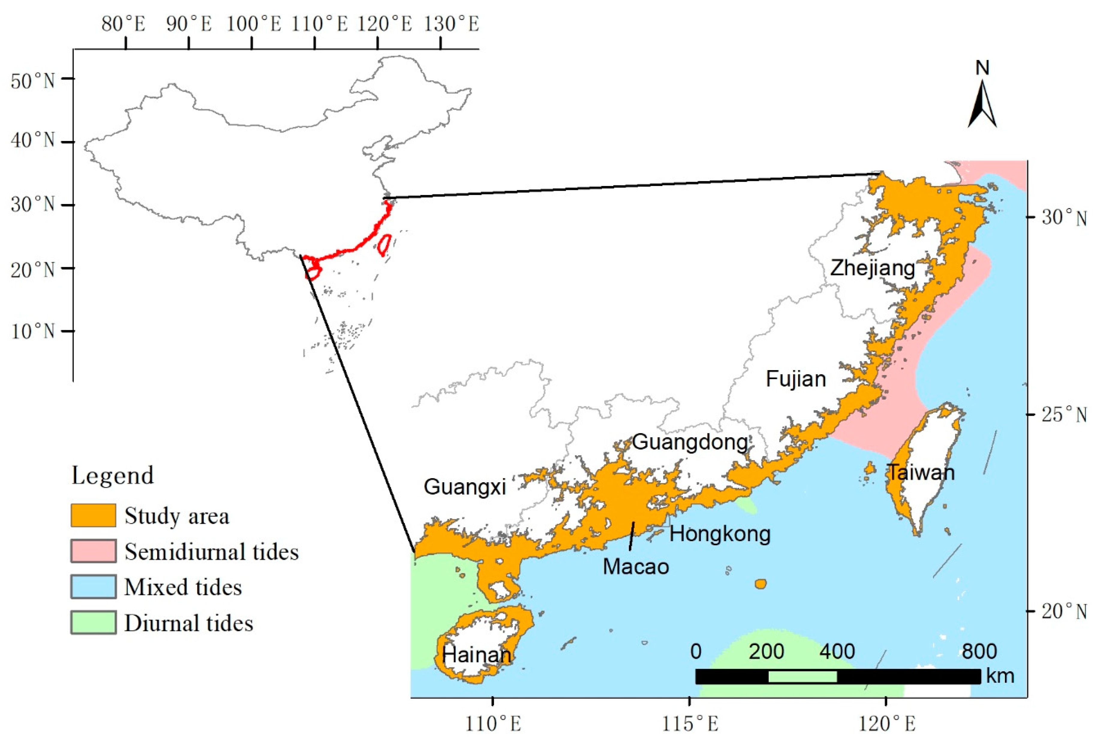
The hypothesis was validated along the coastal area of China. In this region, mangroves are scattered along the lengthy coastlines from their most suitable tropical zone climate to the marginal subtropical zone (Figure 1). Within the area, abundant tidal patterns (i.e., diurnal, semidiurnal, and mixed tides) enrich the interaction between seas and rivers [36]. The variety of climate and salinity combinations leads to a great diversity in mangroves, with 24 species accounting for about one-third of the total true mangrove species existing worldwide [11,37]. The mangrove species that cannot live in a terrestrial or aquatic habitat are regarded as one category in current classifications [23], combined with their varying canopy density and physical appearance, the difficulty of accurately classifying the mangroves of China is exacerbated. Numerous aquaculture ponds and abundant forms of land use also result in large areas of vegetation near water, which is the basis of validating the proposed hypothesis.
A preliminary area (3.83° N to 31.18° N, 108.02° E to 122.95° E) was divided into 1 × 1′ cells. To fully capture the area in which mangroves may grow in southern China, the cells were intersected with low-lying areas filtered by the ETOPO1 global relief model [38], a low-lying area identified by AW3D30 [39] and the most recent tidal flat map of southern China for 2017 [36]. Then, the cells of these three sources were merged by union to form the study area.
2.3. Data Sources
2.3.1. Sentinel Images and DEM
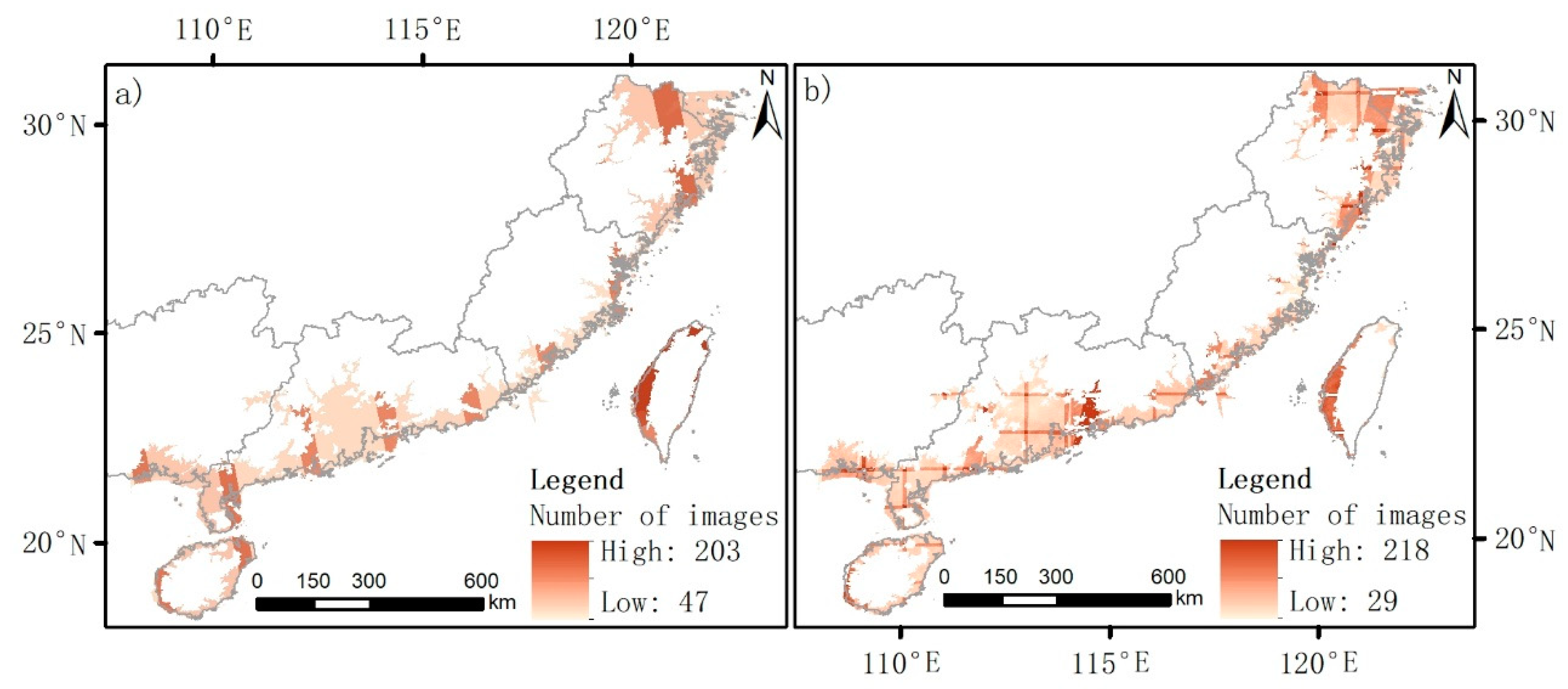
Features were calculated from Sentinel-1 SAR and Sentinel-2 MSI images (Figure 2), which, with their constellations of twin satellites developed by the European Space Agency, provide higher temporal resolutions than Landsat-8. The Sentinel-1 SAR images are sensitive to the physical properties of the land surface (e.g., the canopy structure of vegetation) and have two bands which can penetrate clouds: the vertical transmit and vertical receive (VV) polarization bands and the vertical transmit and horizontal receive (VH) polarization bands. The Sentinel-2 MSI images are sensitive to bio-chemical properties (e.g., chlorophyll content) and have ten bands: three visual bands (B2, B3, B4), one near infrared band (B8), four red-edge bands (B5, B6, B7, B8A), and two shortwave infrared band (B11, B12). AW3D30, produced using ALOS scenes acquired from 2006 to 2011 and released in 2016, was selected to derive terrain-based features because of its high vertical accuracy of about 5 m [40,41,42]. In this study, AW3D30 was used to provide terrain information of low-lying vegetation habitats, which is one of the characteristics of mangroves [14,18].
To describe land covers by their frequency over a time period (e.g., greenness frequency in Chen, et al. [14]), time series of Sentinel-2 images from July 2017 to July 2019 were used. Other features were calculated using a median composite image [43] derived from the same period to reduce noise and cloud effects. The optical images were masked using the QA60 band. All the data were accessed and processed on the Google Earth Engine cloud computing platform, which includes SAR images of Sentinel-1 (https://developers.google.com/earth-engine/datasets/catalog/COPERNICUS_S1_GRD (accessed on 24 December 2020)), top-of-atmosphere reflectance data of Sentinel-2 (https://developers.google.com/earth-engine/datasets/catalog/COPERNICUS_S2 (accessed on 24 December 2020)), and AW3D30 data (https: //developers.google.com/earth-engine/datasets/catalog/JAXA_ALOS_AW3D30_V1_1 (accessed on 24 December 2020)).
2.3.2. Features Used in the Experiments
The features used in the experiments were collected in existing mangrove mapping studies and then categorized into two types based on whether a feature is specifically designed for identifying mangroves, that is, general features and specific features (Table 1). General features are for general purpose, such as VV band from Sentinel-1 SAR used in mapping mangroves in China by Hu, et al. [28], elevation from AW3D30 used in mapping mangroves in China by Zhao and Qin [18], NDVI, the enhanced vegetation index (EVI), and land surface water index (LSWI) from Sentinel-2 MSI used in mapping mangroves in China by Chen, et al. [14]. Based on the literature on mangrove classification, 39 general features were collected, including 15 single band features from Sentinel-1 and -2 images using a median composition of time-series images of the same time period as well as DEM-derived information [18,19,44,45], nine band ratio features extended from [46,47], and 15 index features as in [17,48,49,50].
A number of 15 specific features which are sensitive to mangroves and mangrove environments were also collected. Nine among them are index features: mangrove index (MI) from Winarso, et al. [51], the mangrove forest index (MFI) from Jia, et al. [52], the mangrove vegetation index (MVI) from Baloloy, et al. [31], the discriminant normalized vegetation index (DNVI) from Manna and Raychaudhuri [53], the combined mangrove recognition index (CMRI) from Gupta, et al. [54], mangrove discrimination index 2 (MDI2), mangrove discrimination index 1 (MDI1), the wetland forest index (WFI) from Wang, et al. [17], and the forest discrimination index (FDI) as modified in Kamal, et al. [55]. The remaining six indices describe mangroves using frequency over a time period, not only the frequencies of greenness (FG), canopy coverage (FC), and tidal inundation (FT), but also the ratio between these frequencies and mean NDVI was extracted since the thresholds of the phenology-based algorithm were calculated according to the mean NDVI as in Chen, et al. [14].
2.3.3. Reference Mangrove Map Used in the Experiments
The mangrove map of China for 2019 was used as the reference map to validate the hypothesis. By combing the classification results from Sentinel images and DEM (i.e., a subset of the features in Table 1), and the corrections including empirical constraints based on a tidal flat map and visual inspections based on the Google Earth images, the reference map achieved an overall accuracy of 96.4 ± 0.3% based on validation datasets, and an accuracy of 96.2% based on a total of 1096 field sample plots [56]. This map is open-accessed at the Science Data Bank (http://0-www-dx-doi-org.brum.beds.ac.uk/10.11922/sciencedb.00245 (accessed on 7 January 2021)). The mangrove map produced mainly by interpreters through visual inspections and field investigation (such as the mangrove map by [57]) was not chosen as the reference mangrove map. This is because the way such a mangrove map is produced is comparatively different from the classification-based way focused in this study. For example, the neighboring mangrove patches (even including some nearby tidal flats) will be sketched as one patch by human, but the classification algorithms will not simplify these patches to be one.
2.4. The First Experiment: Classification with the Two Schemes When Using the Same Total Features
2.4.1. Standard Classification Scheme and Sampling
A revised classification scheme (Table 2) from Zhao and Qin [18] was reused, as well as the samples they collected (http://0-www-dx-doi-org.brum.beds.ac.uk/10.11922/sciencedb.00279 (accessed on 7 January 2021)). For each category, 1200 sample points were randomly selected to generate the training dataset, which was used to describe the categories. The samples were the same size to guarantee the equal probability of each category to be trained by the random forest algorithm. The remaining samples in each category were added to the validation set.
2.4.2. New Classification Scheme and Sampling
Considering phenological characteristics of vegetation near water that the herbaceous senesces in winter and the woody is evergreen, the two categories were added into the typical scheme to build the new classification scheme (Table 3). Following the definition of non-mangrove vegetation near water in Section 2.1, a total of 2776 samples for woody vegetations near water and 2931 samples for herbaceous vegetations near water were manually collected based on high-resolution Google Earth images. For each of the two categories, 1200 samples were randomly selected and they were combined with the former training dataset to generate the new training dataset; the remaining samples were added to the validation set.
2.4.3. Classification under the Two Schemes
As an ensemble classifier with high computation efficiency, RF is widely used in land cover classification, including mangrove classification [19,35,58]. Among the RF parameters, the number of trees and the number of input variables randomly chosen at each node need to be determined by the user. Following Belgiu and Drăguţ [35], the number of trees was set to 500, and the number of input variables randomly chosen at each node was set to be seven. Same parameters were used for classifications under the two schemes. The classifications were executed utilizing 54 features (see Section 2.3.2) on the GEE platform.
2.5. The Second Experiment: Classification with the Two Schemes Using the Optimal Features
2.5.1. Feature Selection
The optimization of features was achieved through feature selection, which can approximate the optimal feature subset for each classification scheme. A genetic algorithm (GA) [45,59,60,61] was used, using the genalg package [62] in the R environment (Vienna, Austria). The algorithm, inspired by the theory of evolution, can find a global optimum by selection, crossover, and mutation [63,64]. To select the features in this study, a population was randomly initialized with a certain number of individuals. An individual representing a candidate solution for feature selection was composed of a total of 54 bits. The bits of 1 or 0 (i.e., individual genes) indicate whether the corresponding features are selected or not. Then, each individual was evaluated by a fitness function. Individuals with high fitness values were more likely to be chosen for reproduction (i.e., selection). During the reproduction, a pair of individuals was selected to swap a corresponding segment of the bits (i.e., crossover) and the reproduced individuals were randomly selected to change one randomly chosen bit (i.e., mutation). Finally, the reproduced individuals formed a new generation. The cycle of evolution and reproduction was repeated until meeting a stopping criterion.
The fitness function used to evaluate the individuals is important, as it guides the evolution in GA. To be consistent with the RF-based classifications, the out-of-bag error, used to estimate the performance of the trained RF model, was used as a fitness value to evaluate an individual (i.e., a candidate combination of features). The out-of-bag error was calculated using out-of-bag samples, which are subsets of training samples by a random sample with replacement [65]. Due to the randomness in sampling, the fitness value varies for a given combination of features. To solve the problem, the evaluation procedure was monitored to record individuals and corresponding fitness values. An individual appearing several times in the iteration with varying fitness values could be represented by a mean fitness value to reduce the effect of randomness. Moreover, the best combination of features was determined by voting a set of top 10 individuals sorted by mean fitness value after trial and error, to increase the robustness of the selected features. The GA converged quickly using the default parameters (population size = 200, generation number = 100, mutation rate = 1%). The number of 7 to 15 genes was tested to obtain different feature combinations for each scheme.
The optimal features for each scheme were determined by classification performances in case area. The performance was measured by the sensitive rate (i.e., the rate between number of mangrove pixels and number of pixels classified as mangroves) in reference to a mangrove map. When sensitive rates were close, the spatial distribution of mangrove patches was used to determine the best pre-classification result, thus the corresponding features were chosen as the optimal features. When a reference map is absent, visual inspections can be used to determine the best pre-classification result corresponding to the selected features.
After the feature selection, there are 12 optimal features for the standard classification scheme (B2, B5, VV, VH, elevation, sr9, NDWI, NDRE4, DNVI, MDI2, MVI, FG), and 10 optimal features for the new classification scheme (B5, VV, elevation, sr6, sr8, FDI, LSWI, mNDWI2, NDRE4, FG).
2.5.2. Classification Using the Optimal Features under the Two Schemes
The classification schemes and training datasets were the same as in Section 2.4. The RF was used in classifications using the optimal features on the GEE platform, with the number of trees set to 500 and the number of input variables randomly chosen at each node to be three.
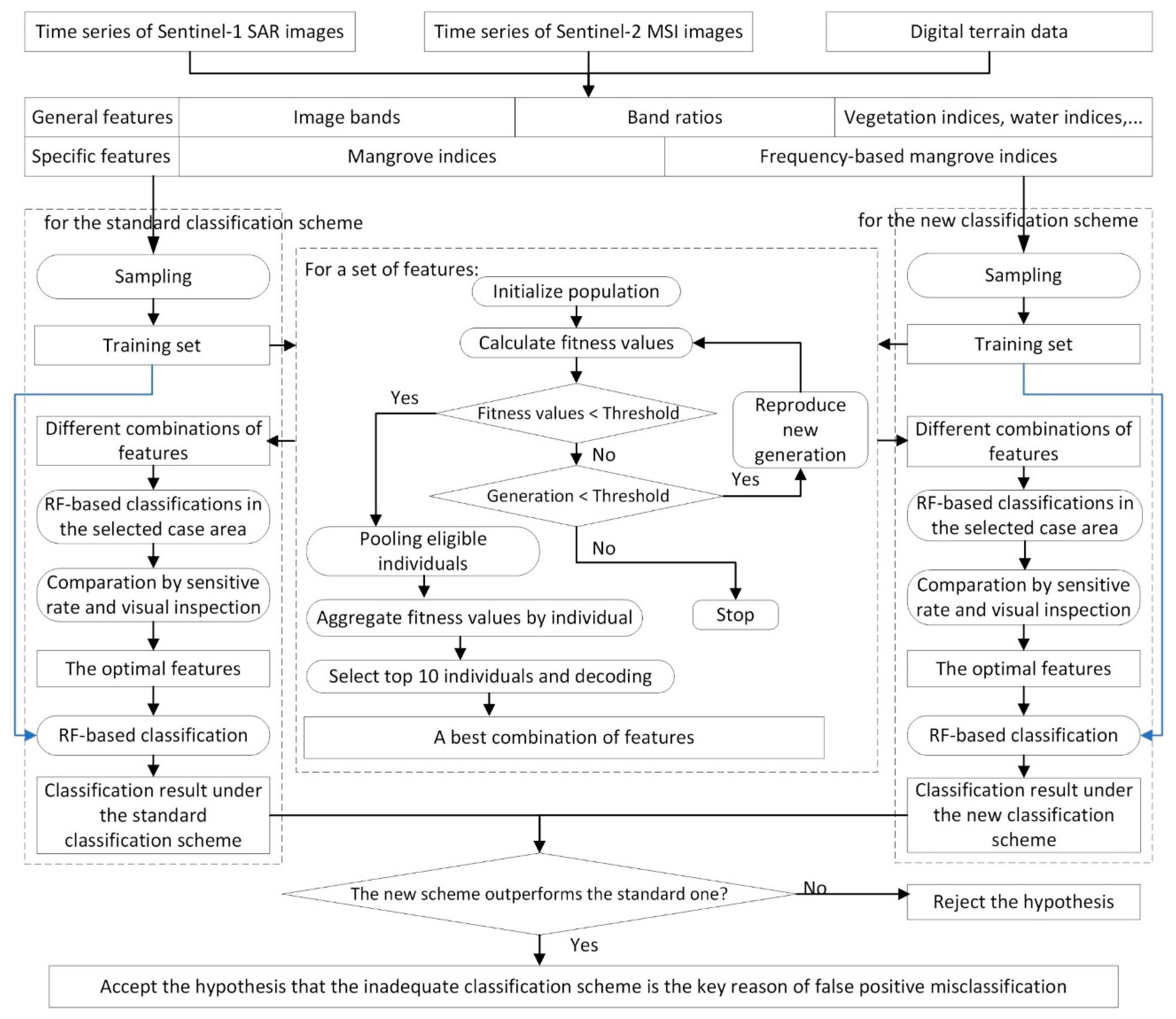
Figure 3 shows the detailed workflow for the two experiments. The first experiment does not include a feature selection procedure (i.e., the blue arrows that skipped feature selection), thus validates the hypothesis using exactly the same features. The second experiment validates the hypothesis in approximate optimal feature space. The feature selection was performed using R, and classifications were performed using the GEE platform.
2.6. Evaluation and Hypothesis Validation
2.6.1. Evaluation Methods
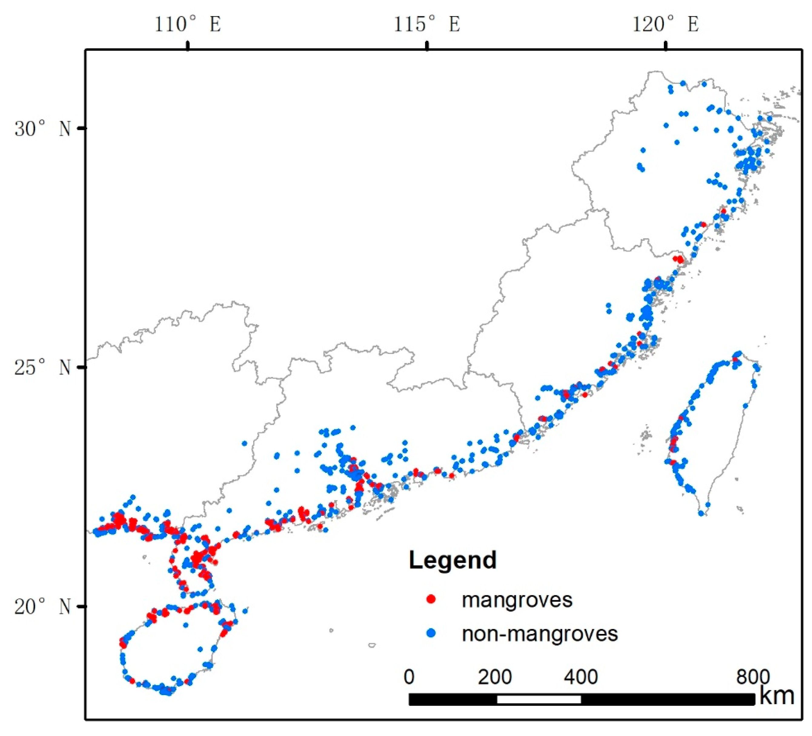
The classifications with the two schemes were evaluated through a quantitative accuracy assessment based on the validation dataset (Figure 4). Considering that the difference between classification schemes before and after inclusion of new categories will affect the evaluation [66], and as well that the mangrove category is the focus of this study, the evaluation was performed based on two categories (i.e., mangroves and non-mangroves). A number of 900 mangrove validation samples were randomly selected in a mangrove map, which was produced mainly by interpreters through visual inspections and field investigation (see Section 2.3.3). Non-mangrove validation samples with the same size were selected by stratified random sampling in the prepared validation set (i.e., a total number of 6102 samples). All of the four classification results use the same validation dataset. According to the formula provided by James, et al. [67] and Murray, et al. [68], the theoretical number of validation samples should be 1537 for such an area, thus the generated validation set with 1800 samples in this study should be reliable. The confusion matrices for each experiment were provided to measure the two classifications with different schemes. In each confusion matrix, the producer’s accuracy and user’s accuracy were calculated for mangroves and non-mangroves, as well as the overall accuracy for all classes [66].
2.6.2. Hypothesis Validation Methods
As the core of this study is to reveal the key reason for false positive misclassification, the validation focused on the false positive part. The number of false positive pixels of mangroves was used for comparison (The false positives and false negatives below are for mangroves). The false positive pixels were judged pixel by pixel based on the reference mangrove map. If a pixel was non-mangrove in the reference map and meanwhile was mangroves in the classification result, it was regarded as a false positive pixel. To reveal local false positive characteristics of the classification results, the pixels misclassified as mangroves within each 1 × 1 km cells were summarized with a method of stratified summary statistics (i.e., the sum of number of misclassified pixels fell into different intervals defined by breaks 0.1%, 1%, 5%, 10%, 20%, 30%, and 40%). The number of cells in each false positive rate interval was compared in the whole area by the 100% stacked column chart and in case areas by the spatial distribution map (Figure 5). A small percentage of intervals greater than zero and a large proportion of false positive rates equal to zero both mean a better performance. In addition to the summarized local statistics, the direct classification results in two selected subset areas were also compared by visual inspections (Figure 5); their false positive pixels serve as a measure of quantitative evaluation.
If the new scheme outperformed the standard scheme in each experiment by the quantitative and qualitative validations, the hypothesis is accepted.
3. Results
3.1. Evaluation Results of the Classifications
3.1.1. Classification Results Using the Same Total Features in the First Experiment
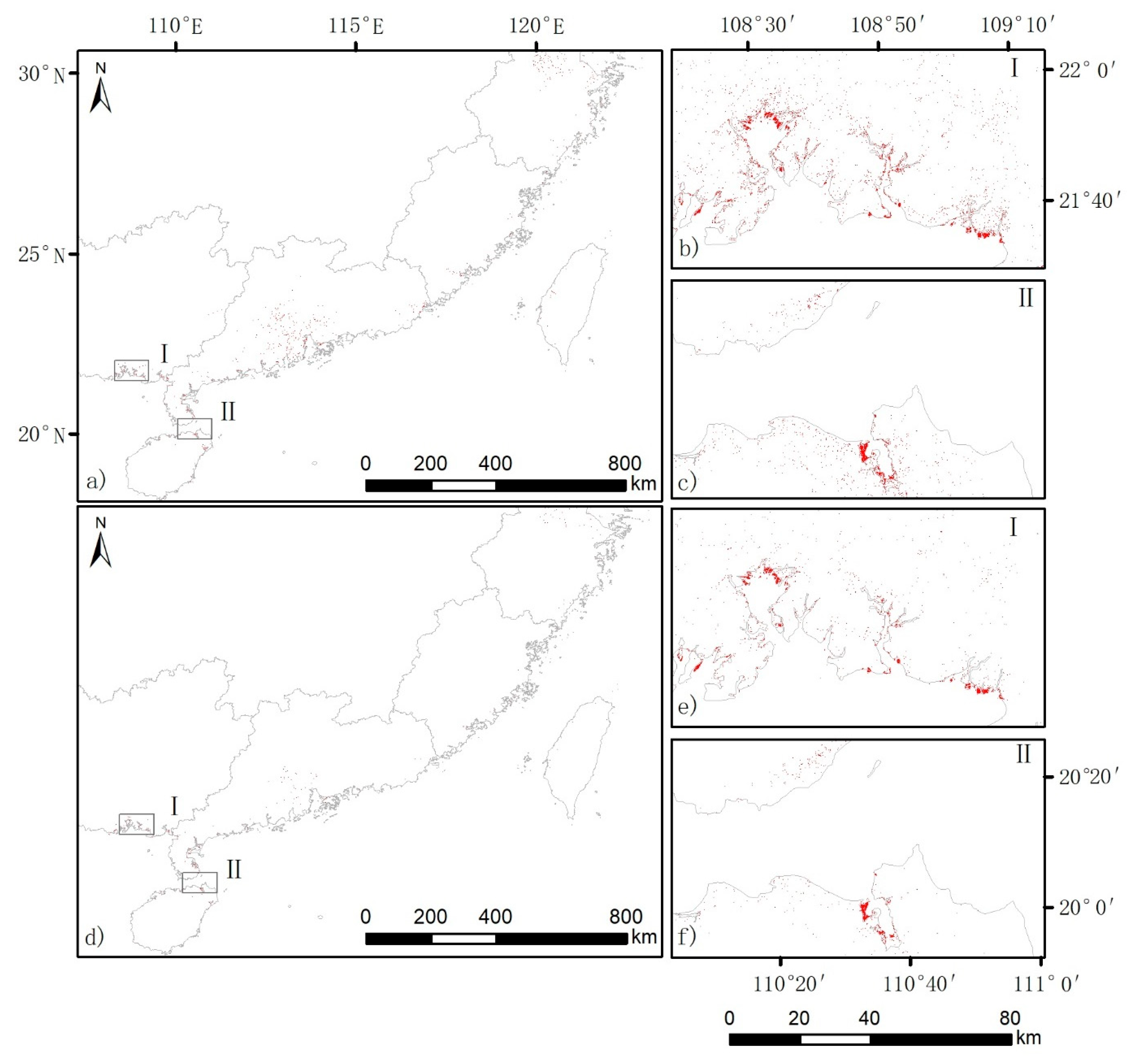
As mangroves are the focus in this study, other categories were excluded in Figure 6. The main maps (Figure 6a,d) show that the mangroves along the coast occupy areas too small to be seen at full scale, and the zoomed-in maps show a wide spread of mangrove patches.
The confusion matrices of the classifications without corrections are shown in Table 4. After the inclusion of non-mangroves near water, the overall accuracy increased from 75.8% to 80.8%. Both the producer’s accuracy and user’s accuracy showed that the commission error (i.e., non-mangroves misclassified as mangroves) was reduced at an expense of a slightly increased omission error (i.e., mangroves misclassified as non-mangroves). The improvement on the commission error when adopting the new scheme was consistent with visual judgement, that is, the classification result with the new scheme had a cleaner and tidier distribution of patches classified as mangroves than that with the standard scheme (Figure 6b,e).
3.1.2. Classification Results Using the Optimal Features in the Second Experiment
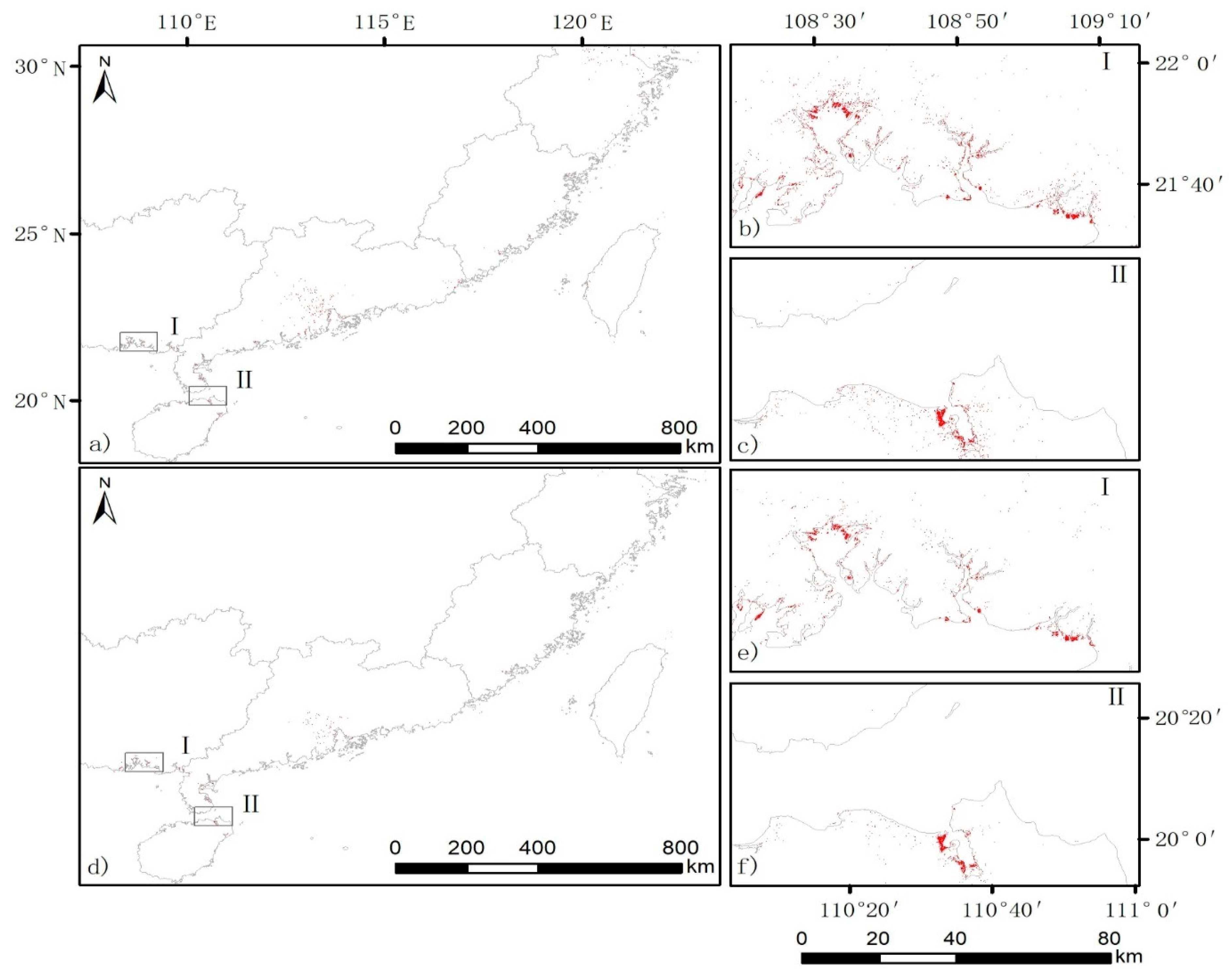
After feature selection, the classifications improved (Figure 7). Similar to classifications in the first experiment, the classification result with the new scheme outperformed the one with the standard scheme by visual inspections (Figure 7b,e).
The confusion matrix and the corresponding statistics are shown in Table 5. Similar to results in the first experiment, the overall accuracy increased from 76.4% to 81.1% after the inclusion of non-mangroves near water. For mangroves, the commission error has a reduction of 17.3% with an increment of omission error of 6.3%. The error matrices support the improvement originated from the inclusion of new categories.
3.2. Validation Results of the Hypothesis
In terms of overall performance, the number of false positive pixels reduced from 16,767,422 to 4,805,313 because of the inclusion of the two categories in the first experiment, with a reduction rate of 71.3%. After the same total features were changed to optimal features approximating the optimal feature subset, the number of false positive pixels reduced from 11,835,120 to 3,993,705 in the second experiment, with a reduction rate of 66.3%. Results from both experiments support the hypothesis to be true.
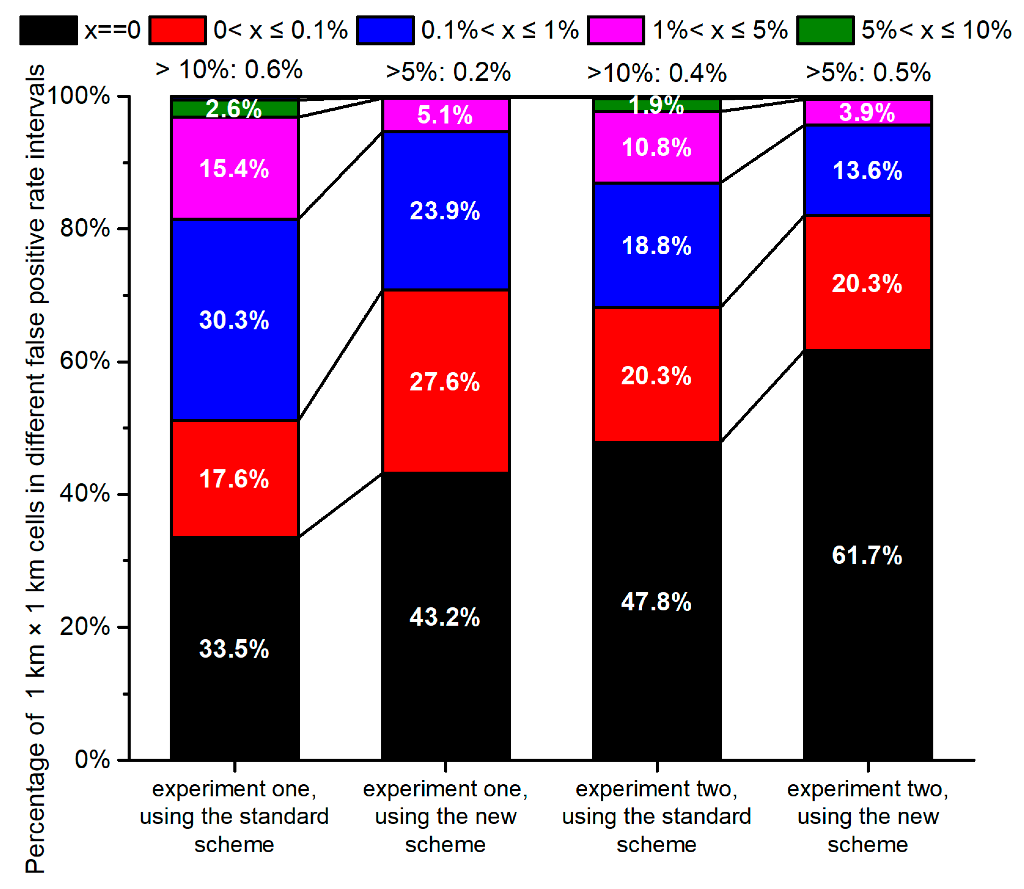
In view of the local false positive characteristics, the 100% stacked column chart (Figure 8) showed that in each experiment the classification result with the new scheme outperformed that with the standard scheme. After inclusion of the two categories, the percentage of cells with a zero false positive rate increased by 9.7% in the first experiment, and it increased by 13.9% in the second experiment. The percentage of each interval greater than 0.1% decreased in varying degrees, and the percentage of cells having a false positive rate greater than 1% deceased from 18.6% to 5.3% in the first experiment, while the percentage decreased from 13.1% to 4.4% in the second experiment.
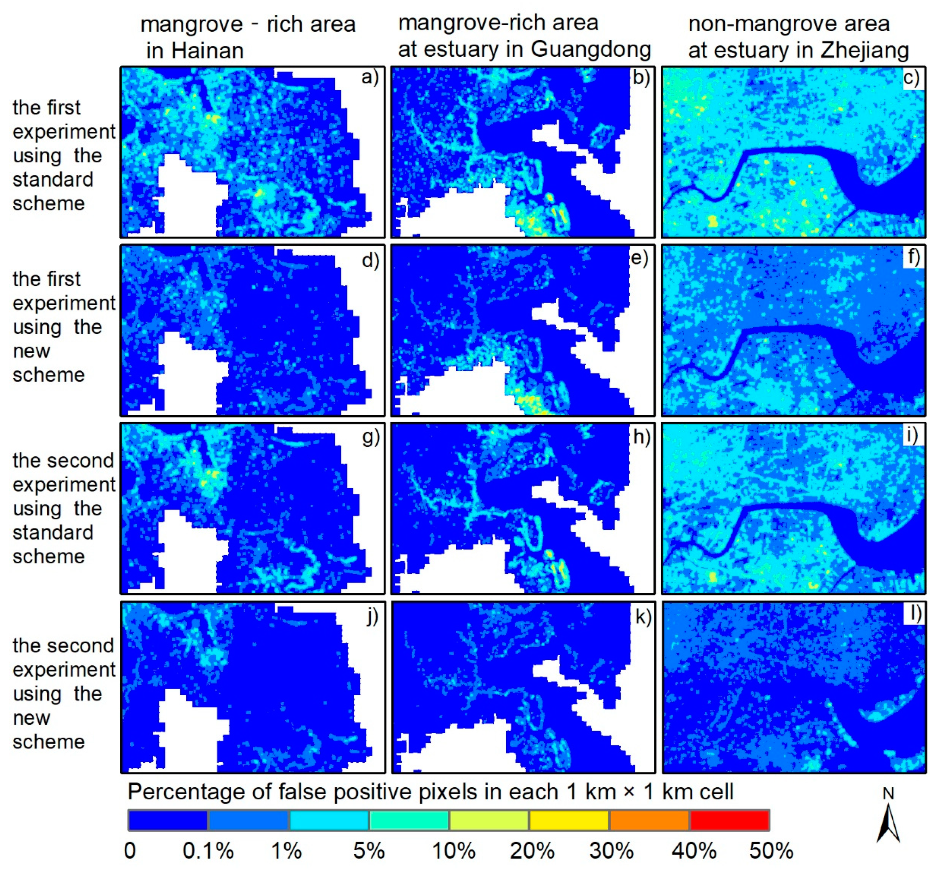
The spatial distribution of percentage of false positive pixels in each 1 × 1 km cell is in Figure 9. In the first experiment, the inclusion of the two categories suppressed false positive patches (e.g., Figure 9a,d). The suppression was more significant in the second experiment after converting from the standard scheme to the new scheme (e.g., Figure 9h,k). Such an improvement can also be because this experiment utilized optimal features to approximate the optimal feature subset, thus to balance the probability of a selected feature to be effective. The local characteristics of false positive pixels support the hypothesis to be true, by means of summary of the whole area and by means of spatial distribution in the case areas.
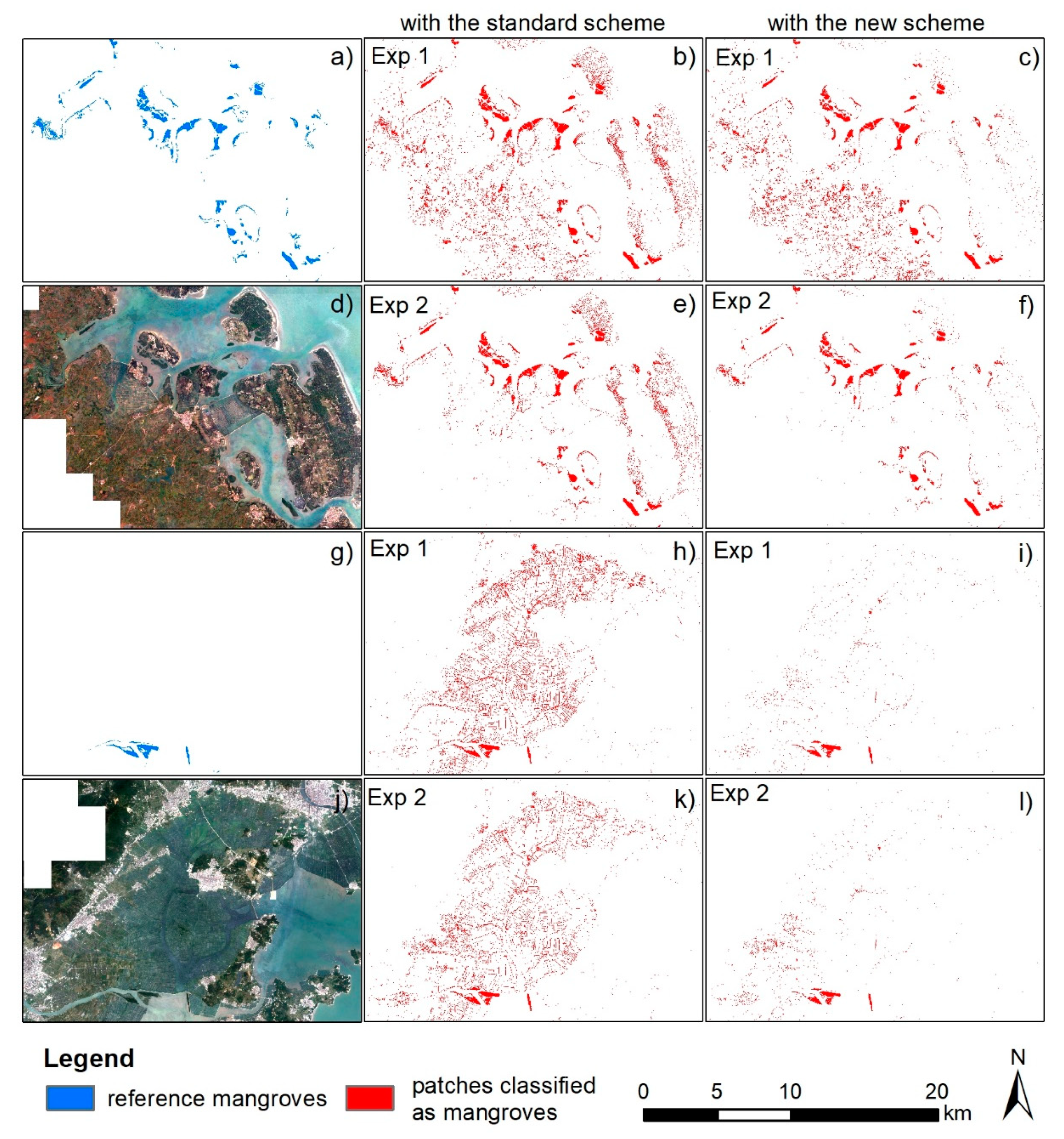
The direct classification results in two selected case areas in two experiments are shown in Figure 10, and corresponding sum statistics of the false positive pixels are shown in Table 6. By visual inspections, the inclusion of the two categories had significantly improved the classification results, which was more apparent in the subset area B dominated by aquaculture (Figure 10h–l). The improvement in the subset area A in the first experiment was not so apparent as in the second experiment. The quantitative statistics showed that the false positive pixels were reduced by 27.1% in the subset area A in the first experiment by converting from the standard scheme to the new scheme, and others were reduced by more than 82.9% through the conversion. The direct classifications support the hypothesis to be true by means of visual inspections and quantitative statistics.
In summary, the hypothesis was proven to be true in three levels of validation in the two experiments, including total number of false positive pixels in the whole area, the proportion and distribution of 1 × 1 km cells with false positive pixels falling into different intervals, and the reduction rate and distribution of false positive pixels in direct classifications in two selected subset areas.
4. Discussion
4.1. Improvement from the Inclusion of New Categories Outperforms That from Increasing Sample Size
Note that the classification accuracy can also be improved by increasing the training sample size [69]. If the improvement from increasing the sample size is similar to that from inclusion of new categories, the hypothesis should be modified from the current one to state that the inadequate consideration of non-mangrove vegetation near water is one of the (key) reasons for false positive misclassification.
This issue is discussed using the first experiment (presented in Section 3.1.1) as an example. We generated a new training dataset with 10,800 samples, which was increased by 50% compared with the training dataset for the standard scheme. Under the same classification scheme (i.e., the standard scheme without consideration of non-mangrove near water), features (i.e., the same total features), algorithm with the parameter-settings (i.e., random forest with a tree number of 500 and a number of input variables randomly chosen at each node of 7), and platform (i.e., the Google Earth Engine), a classification result with a standard classification scheme using the increased training dataset was generated. The number of false positive pixels and number of false negative pixels of the classification result was compared with those from the first experiment (Table 7).
Table 7 shows that the increasement of training sample size can improve the classification result, but the magnitude of improvement is smaller than that from inclusion of new categories (i.e., the non-mangrove near water). As a consequence, the hypothesis can stand as stable.
4.2. Prevalence of False Positive Misclassifications in Existing Studies
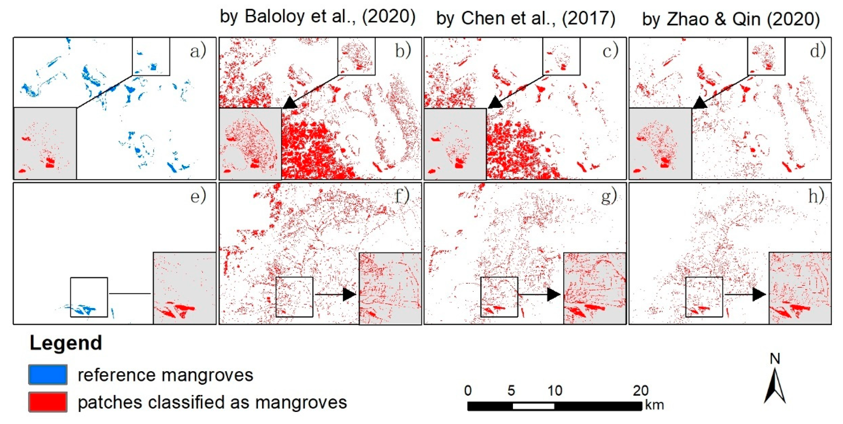
The classification results from three existing studies in two selected subset areas are shown in Figure 11. In the terrestrial, the result from Baloloy, et al. [31] and that from Chen, et al. [14] were spatially similar (Figure 11b,c). The false positive misclassifications in the terrestrial were rarely mentioned in the literature, which may result from the fact that these errors can be eliminated by corrections (such as by applying distance to coastline constraints). In view of vegetation near water, all the approaches failed to give an acceptable result. Though the result from Zhao and Qin [18] seems to be cleaner (Figure 11d), it did not well suppress the non-mangrove vegetation patches near water as that from Chen, et al. [14]. Thus, the false positive misclassifications remain unresolved by various improvements in mangrove classifications.
The classification schemes adopted in the above approaches did not consider an inclusion of new categories (i.e., vegetation near water) to improve the classifications. Mangroves live between terrestrial and marine conditions, where natural and in artificial wetlands are abundant. Mangroves swamps have the characteristics of water inundation, which are similar to salt marshes, lands cultivated for rice during transplanting phase to early vegetative growth phase, and edges of aquaculture ponds. The situation was exacerbated by mixed pixels that vegetation near any water will mix their spectrums to be similar to that having the water inundation characteristics. As a consequence, the non-mangrove near water ignored by standard classification scheme tends to be allocated to be mangroves [70]. Thus, the separability between mangroves and these similar non-mangrove pixels (i.e., wetlands pixels, mixed pixels) is the key to resolve the false positive misclassifications.
The inclusion of the new categories provides a new way to significantly alleviate the prevalent false positive misclassifications in existing studies (zoom-in figures of Figure 11). The included categories drive the classifier to partition them out from the mixture including mangroves and false positive pixels. Such a mandatory partition may result in some pixels previously classified as mangroves as being classified into the new categories (i.e., the reduction of producer’s accuracy), meanwhile a much larger number of systematic misclassified pixels were corrected to be classified into the new categories (i.e., significant reduction on the number of false positive pixels). This phenomenon can be called the shunting effect of the inclusion of new categories, which may explain the mechanism of the improvement in this study.
4.3. Implications to other Mangrove Classification Approaches
In this study, the false positive misclassifications have been significantly reduced with a reduction rate of 71.3% using the new scheme or a rate of 66.3% using the new scheme and feature selection. This improvement is easy to implement in classifications by introducing the new categories to consider vegetation near water that is defined as vegetation within one pixel (i.e., 10 m for Sentinel images) from water bodies.
The false positive misclassifications are one of the main sources of mangrove map inconsistencies [22,56,71,72,73]. Due to empirical constraints that relied on human experience, researchers applied varied constraints with different thresholds (e.g., Hu, et al. [19] used a 10 km distance to the coastline to delineate the potential mangrove areas form the terrestrial, while [14] used a 15 km distance to the coastline). Furthermore, these coarse constraints cannot delineate the false positive patches nearing the mangroves or the sea, such as edges of aquaculture ponds. Thus, the results after corrections need further visual inspections. The widespread occurrence of false positive patches means exhaustive visual inspections, because the visual inspections include three tasks: checking results by empirical constraints, fixing false positive patches that escaped from the constraints, and correcting false negative patches. Fewer false positive misclassifications will shrink the search space for visual inspections, improve the processing efficiency, and reduce participation of labors that have different experience on identifying mangroves, thus increasing the accuracy of mangrove maps. When both mangrove maps approximate the true distribution of mangroves, the consistency problem will be resolved.
5. Conclusions
In this paper, by analyzing the direct classifications from existing RS-based studies on large-area mangrove classifications, a hypothesis that an inadequate classification scheme is the key reason for the false positive misclassification in large area mangroves classifications was proposed. To validate the hypothesis, new categories (i.e., woody vegetations near water, and herbaceous vegetations near water) defined as vegetation within one pixel (i.e., 10 m for Sentinel images) from water bodies were introduced into a standard classification scheme, and thus formed a new classification scheme. In controlled conditions, two experiments in China were conducted on the Google Earth Engine cloud computing platform to derive direct classification results from the two schemes for the year 2018, between which the first experiment using the same total features, and the second experiment using the optimal features to balance the probability of a selected feature to be effective for current scheme. In reference to a mangrove map, the inclusion of the new categories reduced the false positive pixels with a rate of 71.3% in the first experiment, and a rate of 66.3% in the second experiment. The hypothesis was also quantitatively and qualitatively validated by the proportion and distribution of 1 × 1 km cells with false positive pixels falling into different intervals, and by the reduction rate and distribution of false positive pixels in direct classifications in two selected subset areas. All of the three levels of validation in the two experiments support the hypothesis as true.
To the best of our knowledge, this research was the first to reveal and validate the key underlying reason of false positive misclassifications in large-area mangrove classifications. The experiments in this study significantly suppressed the false positive pixels by forcing classification algorithms to partition the false positives out from mangroves after inclusion of the new categories. A significant reduction of false positive pixels will shrink the search space for visual inspections, improve the processing efficiency, and reduce participation of labors, thus to increase the accuracy of mangrove maps. The validated hypothesis can be easily applied to other studies by introducing the new categories.
In the future, the focus will be on the simplification of the multi-class schemes to increase the efficiency in applying the validated hypothesis, and the increase of features by time-series images to further decrease the false positive misclassifications in mangrove classification.
Author Contributions
Conceptualization and writing, C.Z. and C.-Z.Q.; methodology and validation, C.Z.; funding acquisition, C.-Z.Q. All authors have read and agreed to the published version of the manuscript.
Funding
This research was funded by the Science and Technology Basic Resources Investigation Program of China, grant No. 2017FY100706; and the Chinese Academy of Sciences, grant No. XDA23100503.
Data Availability Statement
Google Earth Engine (https://code.earthengine.google.com/, accessed on 14 June 2021) is a free and open platform. All data, models, or code generated or used during this study are available from the corresponding author upon request. The classification code is also available at https://zenodo.org/record/4759685#.YJ3myu15uUl, accessed on 14 June 2021.
Conflicts of Interest
The authors declare no conflict of interest.
References
- Tomlinson, P.B. Botany of Mangroves; Cambridge University Press: Cambridge, UK, 1986. [Google Scholar]
- Wang, L.; Mu, M.; Li, X.; Lin, P.; Wang, W. Differentiation between true mangroves and mangrove associates based on leaf traits and salt contents. J. Plant Ecol. 2010, 4, 292–301. [Google Scholar] [CrossRef] [Green Version]
- Lugo, A.E.; Snedaker, S.C. The ecology of mangroves. Annu. Rev. Ecol. Syst. 1974, 5, 39–64. [Google Scholar] [CrossRef]
- Spalding, M.; Blasco, F.; Field, C. World Mangrove Atlas; International Society for Mangrove Ecosystems: Okinawa, Japan, 1997; Available online: https://www.unep-wcmc.org/resources-and-data/world-mangrove-atlas-1997 (accessed on 14 June 2021).
- Donato, D.C.; Kauffman, J.B.; Murdiyarso, D.; Kurnianto, S.; Stidham, M.; Kanninen, M. Mangroves among the most carbon-rich forests in the tropics. Nat. Geosci. 2011, 4, 293–297. [Google Scholar] [CrossRef]
- Murdiyarso, D.; Purbopuspito, J.; Kauffman, J.B.; Warren, M.W.; Sasmito, S.D.; Donato, D.C.; Manuri, S.; Krisnawati, H.; Taberima, S.; Kurnianto, S. The potential of Indonesian mangrove forests for global climate change mitigation. Nat. Clim. Chang. 2015, 5, 1089–1092. [Google Scholar] [CrossRef]
- Vo, Q.T.; Kuenzer, C.; Vo, Q.M.; Moder, F.; Oppelt, N. Review of valuation methods for mangrove ecosystem services. Ecol. Indic. 2012, 23, 431–446. [Google Scholar] [CrossRef]
- Rahman, A.F.; Dragoni, D.; Didan, K.; Barreto-Munoz, A.; Hutabarat, J.A. Detecting large scale conversion of mangroves to aquaculture with change point and mixed-pixel analyses of high-fidelity MODIS data. Remote Sens. Environ. 2013, 130, 96–107. [Google Scholar] [CrossRef]
- Giri, C.; Zhu, Z.; Tieszen, L.L.; Singh, A.; Gillette, S.; Kelmelis, J.A. Mangrove forest distributions and dynamics (1975–2005) of the tsunami-affected region of Asia. J. Biogeogr. 2007, 35, 519–528. [Google Scholar] [CrossRef]
- Richards, D.R.; Friess, D.A. Rates and drivers of mangrove deforestation in Southeast Asia, 2000–2012. Proc. Natl. Acad. Sci. USA 2016, 113, 344–349. [Google Scholar] [CrossRef] [Green Version]
- Chen, L.; Wang, W.; Zhang, Y.; Lin, G. Recent progresses in mangrove conservation, restoration and research in China. J. Plant Ecol. 2009, 2, 45–54. [Google Scholar] [CrossRef]
- Jia, M.; Wang, Z.; Zhang, Y.; Mao, D.; Wang, C. Monitoring loss and recovery of mangrove forests during 42 years: The achievements of mangrove conservation in China. Int. J. Appl. Earth Obs. Geoinf. 2018, 73, 535–545. [Google Scholar] [CrossRef]
- Giri, C.; Ochieng, E.; Tieszen, L.L.; Zhu, Z.; Singh, A.; Loveland, T.; Masek, J.; Duke, N. Status and distribution of mangrove forests of the world using earth observation satellite data. Glob. Ecol. Biogeogr. 2011, 20, 154–159. [Google Scholar] [CrossRef]
- Chen, B.; Xiao, X.; Li, X.; Pan, L.; Doughty, R.; Ma, J.; Dong, J.; Qin, Y.; Zhao, B.; Wu, Z. A mangrove forest map of China in 2015: Analysis of time series Landsat 7/8 and Sentinel-1A imagery in Google Earth Engine cloud computing platform. ISPRS J. Photogramm. Remote Sens. 2017, 131, 104–120. [Google Scholar] [CrossRef]
- Spalding, M. World Atlas of Mangroves; Routledge: Milton, UK, 2010. [Google Scholar]
- Gao, J. A hybrid method toward accurate mapping of mangroves in a marginal habitat from SPOT multispectral data. Int. J. Remote Sens. 1998, 19, 1887–1899. [Google Scholar] [CrossRef]
- Wang, D.; Wan, B.; Qiu, P.; Su, Y.; Guo, Q.; Wang, R.; Sun, F.; Wu, X. Evaluating the performance of Sentinel-2, Landsat 8 and Pléiades-1 in mapping mangrove extent and species. Remote Sens. 2018, 10, 1468. [Google Scholar] [CrossRef] [Green Version]
- Zhao, C.; Qin, C.-Z. 10-m-resolution mangrove maps of China derived from multi-source and multi-temporal satellite observations. ISPRS J. Photogramm. Remote Sens. 2020, 169, 389–405. [Google Scholar] [CrossRef]
- Hu, L.; Li, W.; Xu, B. Monitoring mangrove forest change in China from 1990 to 2015 using Landsat-derived spectral-temporal variability metrics. Int. J. Appl. Earth Obs. Geoinf. 2018, 73, 88–98. [Google Scholar] [CrossRef]
- Xia, Q.; Qin, C.-Z.; Li, H.; Huang, C.; Su, F.-Z. Mapping mangrove forests based on multi-tidal high-resolution satellite imagery. Remote Sens. 2018, 10, 1343. [Google Scholar] [CrossRef] [Green Version]
- Heumann, B.W. Satellite remote sensing of mangrove forests: Recent advances and future opportunities. Prog. Phys. Geogr. Earth Environ. 2011, 35, 87–108. [Google Scholar] [CrossRef]
- Kuenzer, C.; Bluemel, A.; Gebhardt, S.; Quoc, T.V.; Dech, S. Remote sensing of mangrove ecosystems: A review. Remote Sens. 2011, 3, 878–928. [Google Scholar] [CrossRef] [Green Version]
- Wang, L.; Jia, M.; Yin, D.; Tian, J. A review of remote sensing for mangrove forests: 1956–2018. Remote Sens. Environ. 2019, 231, 111223. [Google Scholar] [CrossRef]
- Sadler, J.; Goodall, J.; Morsy, M.; Spencer, K. Modeling urban coastal flood severity from crowd-sourced flood reports using Poisson regression and Random Forest. J. Hydrol. 2018, 559, 43–55. [Google Scholar] [CrossRef]
- Ryu, S.; Kang, J. Machine learning-based fast angular prediction mode decision technique in video coding. IEEE Trans. Image Process. 2018, 27, 5525–5538. [Google Scholar] [CrossRef]
- Alvarez, I.; Bernard, S.; Deffuant, G. Keep the Decision Tree and Estimate the Class Probabilities Using its Decision Boundary. In Proceedings of the 20th International Joint Conference on Artificial Intelligence, Hyderabad, India, 6–12 January 2007; pp. 654–659. [Google Scholar]
- Alsberg, B.; Goodacre, R.; Rowland, J.; Kell, D. Classification of pyrolysis mass spectra by fuzzy multivariate rule induction-comparison with regression, K-nearest neighbour, neural and decision-tree methods. Anal. Chim. Acta 1997, 348, 389–407. [Google Scholar] [CrossRef]
- Hu, L.; Xu, N.; Liang, J.; Li, Z.; Chen, L.; Zhao, F. Advancing the mapping of mangrove forests at national-scale using Sentinel-1 and Sentinel-2 time-series data with Google Earth Engine: A case study in China. Remote Sens. 2020, 12, 3120. [Google Scholar] [CrossRef]
- Tahmassebi, A.; Gandomi, A.H.; Schulte, M.H.J.; Goudriaan, A.E.; Foo, S.; Meyer-Baese, A. Optimized Naive-Bayes and Decision Tree approaches for fMRI smoking cessation classification. Complexity 2018, 2018. [Google Scholar] [CrossRef]
- Di Gregorio, A. Land Cover Classification System: Classification Concepts and User Manual; LCCS: Fort Worth, TX, USA; Food & Agriculture Org.: Rome, Itlay, 2005; Volume 2. [Google Scholar]
- Baloloy, A.B.; Blanco, A.C.; Ana, R.R.C.S.; Nadaoka, K. Development and application of a new mangrove vegetation index (MVI) for rapid and accurate mangrove mapping. ISPRS J. Photogramm. Remote. Sens. 2020, 166, 95–117. [Google Scholar] [CrossRef]
- Ruttenberg, B.; Granek, E. Bridging the marine–terrestrial disconnect to improve marine coastal zone science and management. Mar. Ecol. Prog. Ser. 2011, 434, 203–212. [Google Scholar] [CrossRef] [Green Version]
- Carr, M.H.; Neigel, J.E.; Estes, J.A.; Andelman, S.; Warner, R.; Largier, J.L. Comparing marine and terrestrial ecosystems: Implications for the design of coastal marine reserves. Ecol. Appl. 2003, 13, 90–107. [Google Scholar] [CrossRef] [Green Version]
- Cao, L.; Chen, Y.; Dong, S.; Hanson, A.; Huang, B.; Leadbitter, D.; Little, D.C.; Pikitch, E.K.; Qiu, Y.; de Mitcheson, Y.S.; et al. Opportunity for marine fisheries reform in China. Proc. Natl. Acad. Sci. USA 2017, 114, 435–442. [Google Scholar] [CrossRef] [Green Version]
- Belgiu, M.; Drăguţ, L. Random forest in remote sensing: A review of applications and future directions. ISPRS J. Photogramm. Remote Sens. 2016, 114, 24–31. [Google Scholar] [CrossRef]
- Zhao, C.; Qin, C.-Z.; Teng, J. Mapping large-area tidal flats without the dependence on tidal elevations: A case study of Southern China. ISPRS J. Photogramm. Remote Sens. 2020, 159, 256–270. [Google Scholar] [CrossRef]
- Li, M.; Lee, S.Y. Mangroves of China: A brief review. For. Ecol. Manag. 1997, 96, 241–259. [Google Scholar] [CrossRef]
- Amante, C.; Eakins, B.W. ETOPO1 Arc-Minute Global Relief Model: Procedures, Data Sources and Analysis; NOAA: Silver Spring, MD, USA, 2009.
- Tadono, T.; Nagai, H.; Ishida, H.; Oda, F.; Naito, S.; Minakawa, K.; Iwamoto, H. Generation of the 30 m-mesh global digital surface model by ALOS PRISM. In Proceedings of the International Archives of the Photogrammetry, Remote Sensing & Spatial Information Sciences, Prague, Czech Republic, 12–19 July 2016; pp. 157–162. [Google Scholar]
- Takaku, J.; Tadono, T.; Doutsu, M.; Ohgushi, F.; Kai, H. Updates of ‘AW3D30’ ALOS global digital surface model with other open access datasets. In Proceedings of the International Archives of Photogrammetry, Remote Sensing and Spatial Information Sciences, Nice, France, 24 August 2020; Volume 43, pp. 183–189. [Google Scholar]
- Tadono, T.; Ishida, H.; Oda, F.; Naito, S.; Minakawa, K.; Iwamoto, H. Precise global DEM generation by ALOS PRISM. ISPRS Ann. Photogramm. Remote Sens. Spat. Inf. Sci. 2014, 2, 71–76. [Google Scholar] [CrossRef] [Green Version]
- Aslan, A.; Rahman, A.F.; Robeson, S.M. Investigating the use of Alos Prism data in detecting mangrove succession through canopy height estimation. Ecol. Indic. 2018, 87, 136–143. [Google Scholar] [CrossRef]
- Gómez, C.; White, J.C.; Wulder, M. Optical remotely sensed time series data for land cover classification: A review. ISPRS J. Photogramm. Remote Sens. 2016, 116, 55–72. [Google Scholar] [CrossRef] [Green Version]
- Bunting, P.; Rosenqvist, A.; Lucas, R.; Rebelo, L.M.; Hilarides, L.; Thomas, N.; Hardy, A.; Itoh, T.; Shimada, M.; Finlayson, C.M. The global mangrove watch—A new 2010 global baseline of mangrove extent. Remote Sens. 2018, 10, 1669. [Google Scholar] [CrossRef] [Green Version]
- Vaiphasa, C.; Skidmore, A.; de Boer, W.F.; Vaiphasa, T. A hyperspectral band selector for plant species discrimination. ISPRS J. Photogramm. Remote Sens. 2007, 62, 225–235. [Google Scholar] [CrossRef]
- Gray, D.; Zisman, S.; Corver, C. Mapping of the Mangroves of Belize; University of Edinburgh: Edinburgh, UK, 1990. [Google Scholar]
- Green, E.P.; Clark, C.D.; Mumby, P.J.; Edwards, A.J.; Ellis, A.C. Remote sensing techniques for mangrove mapping. Int. J. Remote Sens. 1998, 19, 935–956. [Google Scholar] [CrossRef]
- Kaplan, G.; Avdan, U. Sentinel-1 and Sentinel-2 data fusion for mapping and monitoring wetlands. In Proceedings of the International Archives of the Photogrammetry, Remote Sensing and Spatial Information Sciences, Beijing, China, 7–10 May 2018; XLII-3. [Google Scholar]
- Dong, J.; Xiao, X.; Menarguez, M.A.; Zhang, G.; Qin, Y.; Thau, D.; Biradar, C.; Moore, B., III. Mapping paddy rice planting area in northeastern Asia with Landsat 8 images, phenology-based algorithm and Google Earth Engine. Remote Sens. Environ. 2016, 185, 142–154. [Google Scholar] [CrossRef] [Green Version]
- Badgley, G.; Field, C.B.; Berry, J.A. Canopy near-infrared reflectance and terrestrial photosynthesis. Sci. Adv. 2017, 3, e1602244. [Google Scholar] [CrossRef] [Green Version]
- Winarso, G.; Purwanto, A.; Yuwono, D. New mangrove index as degradation health indicator using remote sensing data: Segara Anakan and Alas Purwo case study. In Proceedings of the 12th Biennial Conference of Pan Ocean Remote Sensing Conference, Bali, Indonesia, 4–7 November 2014; pp. 309–316. [Google Scholar]
- Jia, M.; Wang, Z.; Mao, D.; Zhang, Y. A new vegetation index to detect periodically submerged mangrove forest using single-tide Sentinel-2 imagery. Remote Sens. 2019, 11, 2043. [Google Scholar] [CrossRef] [Green Version]
- Manna, S.; Raychaudhuri, B. Mapping distribution of Sundarban mangroves using Sentinel-2 data and new spectral metric for detecting their health condition. Geocarto Int. 2020, 35, 434–452. [Google Scholar] [CrossRef]
- Gupta, K.; Mukhopadhyay, A.; Giri, S.; Chanda, A.; Majumdar, S.D.; Samanta, S.; Mitra, D.; Samal, R.N.; Pattnaik, A.K.; Hazra, S. An index for discrimination of mangroves from non-mangroves using LANDSAT 8 OLI imagery. MethodsX 2018, 5, 1129–1139. [Google Scholar] [CrossRef]
- Kamal, M.; Phinn, S.; Johansen, K. Object-Based Approach for Multi-Scale Mangrove Composition Mapping Using Multi-Resolution Image Datasets. Remote Sens. 2015, 7, 4753–4783. [Google Scholar] [CrossRef] [Green Version]
- Zhao, C.; Qin, C. A detailed mangrove map of China for 2019 derived from Sentinel-1 and -2 images and Google Earth images. Geosci. Data J. 2021. [Google Scholar] [CrossRef]
- Zhang, T.; Hu, S.; He, Y.; You, S.; Yang, X.; Gan, Y.; Liu, A. A fine-scale mangrove map of China derived from 2-meter resolution satellite observations and field data. ISPRS Int. J. Geo-Inf. 2021, 10, 92. [Google Scholar] [CrossRef]
- Li, H.; Jia, M.; Zhang, R.; Ren, Y.; Wen, X. Incorporating the plant phenological trajectory into mangrove species mapping with dense time series Sentinel-2 imagery and the Google Earth Engine platform. Remote Sens. 2019, 11, 2479. [Google Scholar] [CrossRef] [Green Version]
- Vancoillie, F.; Verbeke, L.; Dewulf, R. Feature selection by genetic algorithms in object-based classification of IKONOS imagery for forest mapping in Flanders, Belgium. Remote Sens. Environ. 2007, 110, 476–487. [Google Scholar] [CrossRef]
- Tseng, M.-H.; Chen, S.-J.; Hwang, G.-H.; Shen, M.-Y. A genetic algorithm rule-based approach for land-cover classification. ISPRS J. Photogramm. Remote Sens. 2008, 63, 202–212. [Google Scholar] [CrossRef]
- Duro, D.; Franklin, S.; Dubé, M.G. A comparison of pixel-based and object-based image analysis with selected machine learning algorithms for the classification of agricultural landscapes using SPOT-5 HRG imagery. Remote Sens. Environ. 2012, 118, 259–272. [Google Scholar] [CrossRef]
- Willighagen, E.; Genalg, M.B. R Based Genetic Algorithm. Available online: https://cran.r-project.org/web/packages/genalg/genalg.pdf (accessed on 14 June 2021).
- Goldberg, D.E. Genetic algorithms in Search, Optimization, and MachineLearning; Addison-Wesley Publishing Company: Boston, MA, USA, 1989. [Google Scholar]
- Parker, J.R. Algorithms for Image Processing and Computer Vision; John Wiley & Sons, Inc.: Hoboken, NJ, USA, 1996. [Google Scholar]
- Breiman, L. Random forests. Mach. Learn. 2001, 45, 5–32. [Google Scholar] [CrossRef] [Green Version]
- Congalton, R.G.; Green, K. Assessing the Accuracy of Remotely Sensed Data: Principles and Practices; CRC press: Boca Raton, FL, USA, 2019. [Google Scholar]
- James, G.; Witten, D.; Hastie, T.; Tibshirani, R. An Introduction to Statistical Learning; Springer: New York, NY, USA, 2013; Volume 103. [Google Scholar]
- Murray, N.; Phinn, S.R.; DeWitt, M.; Ferrari, R.; Johnston, R.; Lyons, M.B.; Clinton, N.; Thau, D.; Fuller, R.A. The global distribution and trajectory of tidal flats. Nat. Cell Biol. 2019, 565, 222–225. [Google Scholar] [CrossRef] [PubMed]
- Foody, G.M.; Mathur, A.; Sanchez-Hernandez, C.; Boyd, D. Training set size requirements for the classification of a specific class. Remote Sens. Environ. 2006, 104, 1–14. [Google Scholar] [CrossRef]
- Foody, G.M. Impacts of ignorance on the accuracy of image classification and thematic mapping. Remote. Sens. Environ. 2021, 259, 112367. [Google Scholar] [CrossRef]
- Ruiz-Luna, A.; Acosta-Velázquez, J.; Berlanga-Robles, C.A. On the reliability of the data of the extent of mangroves: A case study in Mexico. Ocean Coast. Manag. 2008, 51, 342–351. [Google Scholar] [CrossRef]
- Friess, D.A.; Webb, E. Bad data equals bad policy: How to trust estimates of ecosystem loss when there is so much uncertainty? Environ. Conserv. 2011, 38, 1–5. [Google Scholar] [CrossRef]
- Friess, D.A.; Webb, E. Variability in mangrove change estimates and implications for the assessment of ecosystem service provision. Glob. Ecol. Biogeogr. 2013, 23, 715–725. [Google Scholar] [CrossRef]
Figure 1.
Map of the study area (adapted from Zhao and Qin [18]). The area covers about half of China’s coastline, including the coastal areas of Zhejiang, Fujian, Guangdong, Guangxi Zhuang Autonomous, Hong Kong, Macao, Taiwan, and Hainan.
Figure 1.
Map of the study area (adapted from Zhao and Qin [18]). The area covers about half of China’s coastline, including the coastal areas of Zhejiang, Fujian, Guangdong, Guangxi Zhuang Autonomous, Hong Kong, Macao, Taiwan, and Hainan.

Figure 2.
Number of Sentinel images per 10 m grid cell for (a) synthetic aperture radar (SAR) data; (b) multispectral instrument (MSI) data after masking clouds with the QA60 band.
Figure 2.
Number of Sentinel images per 10 m grid cell for (a) synthetic aperture radar (SAR) data; (b) multispectral instrument (MSI) data after masking clouds with the QA60 band.

Figure 3.
Workflow for validating the hypothesis. The difference is the first experiment skipped the feature selection procedure using blue arrows, thus validating the hypothesis using the same total features rather than using the optimal features that approximate the optimal feature space.
Figure 3.
Workflow for validating the hypothesis. The difference is the first experiment skipped the feature selection procedure using blue arrows, thus validating the hypothesis using the same total features rather than using the optimal features that approximate the optimal feature space.

Figure 4.
Distribution of sample points in the generated validation dataset.

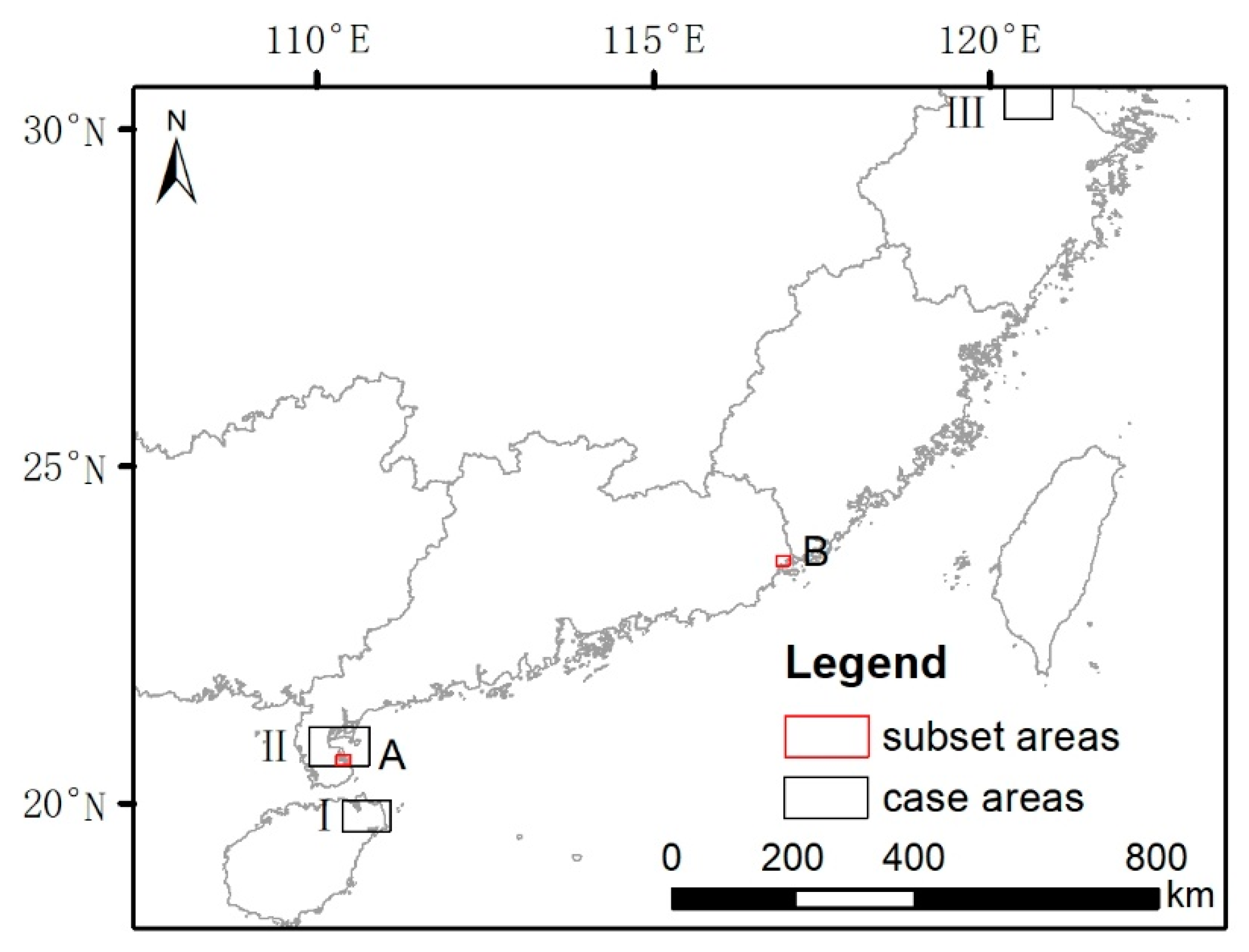
Figure 5.
Locations of selected case areas and subset areas. The case areas are annotated with I, II, and III near the left of the black frames, covering the mangrove-rich area in Hainan, the mangrove-rich area at the estuary in Guangdong, and the non-mangrove area at the estuary in Zhejiang. The subset areas, with the annotation of A and B near the right of the red frames, are smaller than case areas, to depict the direct classifications in detail. The subset area A is a coastal area with complex land covers, and the subset area B is dominated by aquaculture.

Figure 6.
Mangrove classification results in China in 2018 from the two classification schemes: (a) the standard scheme and (d) the new scheme in the first experiment. The results were mapped directly without corrections. Because the mangroves cover a very small portion of the coastal area, the distribution of the classification results are mainly visible in the zoomed-in figures (b,c,e,f), which share the same scale bar.

Figure 7.
Mangrove classification results in China in 2018 from the two classification schemes: (a) the standard scheme and (d) the new scheme in the second experiment. The zoomed-in figures (b–f), share the same scale bar.
Figure 7.
Mangrove classification results in China in 2018 from the two classification schemes: (a) the standard scheme and (d) the new scheme in the second experiment. The zoomed-in figures (b–f), share the same scale bar.

Figure 8.
Percentage of 1 × 1 km cells that fall into different false positive rate intervals defined by breaks 0.1%, 1%, 5%, 10%, 20%,30%, and 40%. The false positive rate of each 1 × 1 km cell is denoted as x in the figure. Percentage of cells with zero false positive rate is displayed in black, and the percentages out of visibility (i.e., the large false positive rate that only accounts for small percentages) are summarized by labels on the top of each bar.

Figure 9.
Percentage of false positive pixels in each 1 × 1 km cell that falls into intervals defined by breaks 0.1%, 1%, 5%, 10%, 20%, 30%, and 40%. The percentage of false positive pixels of different settings of classification scheme and feature selection for mangrove-rich area in Hainan are shown in the left panel as (a,d,g,j), the one for mangrove-rich area at the estuary in Guangdong in the middle panel as (b,e,h,k), and the one for non-mangrove area at the estuary in Zhejiang in the right panel as (c,f,i,l).

Figure 10.
Classification results in the two selected subset areas in two experiments. (Exp1: the first experiment that utilized the same total features in classifications in (b), (c), (h), and (i), and Exp2: the second experiment that utilized the optimal features in classifications to balance the probability that a selected feature was effective for the scheme in (e), (f), (k), and (l). The reference map and corresponding true color composite image from Sentinel-2 for two selected subset areas are shown in left panels, that is, (a) and (d), (g) and (j), respectively.

Figure 11.
Spatial distribution of classification results for selected subset areas by different classification methods. These approaches, including a threshold approach based on the mangrove vegetation index (MVI) by Baloloy, et al. [31] in (b,f), a phenology-based approach by Chen, et al. [14] in (c,g), and a random forest (RF)-based classification approach by Zhao and Qin [18] in (d,h), have varied data sources, features, and classification schemes. Reference maps for subset areas are shown in (a,e). Zoom-in figures are used to compare classification details. The classification results with a classification scheme considering non-mangrove near water using the same total features (i.e., classification results with the new scheme in the first experiment) are shown in zoom-in figures in (a,e).


Table 1.
Features used in the experiments.
| Types | Subtypes | Expressions | ||
|---|---|---|---|---|
| general features | bands | VV, VH, B2, B3, B4, B5, B6, B7, B8, B8A, B11, B12, elevation, slope, aspect | ||
| band ratios | B4/B8, B8/B4, B8/B11, B8/B12, B11/B12, B2/B4, B4/B2, B3/B4, B4/B3 | |||
| other indices | ||||
| specific features | indices | |||
| frequency-based indices | ||||
Note: Shortwave infrared (SWIR) represents B11 and B12, thus two features can be calculated from the expression (e.g., two features were extracted by the expression of the modified normalized difference water index (mNDWI)). RE represents B5, B6, B7, and B8A, thus four features were extracted using the normalized difference red edge (NDRE). The constant value c of near-infrared reflectance of vegetation (NIRv) can be set to 0 or 0.08. For frequency-based indices, the frequency is the ratio between the number of images meeting the criteria and the number of cloud-free images (denoted as ) over the selected period. represents the mean of NDVI over the same period.
Table 2.
The standard classification scheme without consideration of the non-mangrove vegetation near water.
Table 2.
The standard classification scheme without consideration of the non-mangrove vegetation near water.
| Category | Description |
|---|---|
| mangroves | trees, shrubs, and palms that strictly distribute in the intertidal environments [1], which are also referred as true-mangroves [2,13] |
| forests | terrestrial forests, coastal forests, and semi-mangroves that can survive in terrestrial environments [2] |
| cropland | cultivated land that is dominated by rice |
| water | permanent water area that is not affected by seasons |
| tidal flats | bare land that is inundated by high tides and is exposed in low tides |
| impervious surface | sandy and pebble beaches, rocky coasts, and artificial structures (e.g., residential areas, roads) |
Table 3.
The new classification scheme with consideration of the non-mangrove vegetation near water.
Table 3.
The new classification scheme with consideration of the non-mangrove vegetation near water.
| Category | Description |
|---|---|
| mangroves | trees, shrubs, and palms that strictly distribute in the intertidal environments [1] |
| forests | terrestrial forests, coastal forests, and semi-mangroves that can survive in terrestrial environments [2] |
| cropland | cultivated land that is dominated by rice |
| water | permanent water area that is not affected by seasons |
| tidal flats | bare land that is inundated by high tides and is exposed in low tides |
| impervious surface | sandy and pebble beaches, rocky coasts, and artificial structures (e.g., residential areas, roads) |
| forest near water | woody vegetations near water that distribute in the edge of rivers, reservoirs, aquaculture ponds, etc. |
| grass near water | herbaceous vegetations near water that distribute in the edge of rivers, reservoirs, aquaculture ponds, etc. |
Table 4.
Confusion matrices of the classifications without correction with a standard classification scheme and a new classification scheme in the first experiment. The performance of classification with the standard scheme is shown in (a), and that with the new scheme is shown in (b).
Table 4.
Confusion matrices of the classifications without correction with a standard classification scheme and a new classification scheme in the first experiment. The performance of classification with the standard scheme is shown in (a), and that with the new scheme is shown in (b).
| (a) with the standard classification scheme | ||||
| Reference | ||||
| Mangroves | Non-Mangroves | User’s Accuracy | ||
| Classification result | mangroves | 633 | 169 | 78.9% |
| non-mangroves | 267 | 731 | 73.3% | |
| Producer’s Accuracy | 70.3% | 81.2% | ||
| Overall Accuracy | 75.8% | |||
| (b) with the new classification scheme | ||||
| Reference | ||||
| Mangroves | Non-Mangroves | User’s Accuracy | ||
| Classification result | mangroves | 571 | 16 | 97.3% |
| non-mangroves | 329 | 884 | 72.9% | |
| Producer’s Accuracy | 63.4% | 98.2% | ||
| Overall Accuracy | 80.8% | |||
Table 5.
Confusion matrices of the classifications without correction with a standard classification scheme and a new classification scheme in the second experiment. The performance of classification with the standard scheme is shown in (a), and that with the new scheme is shown in (b).
Table 5.
Confusion matrices of the classifications without correction with a standard classification scheme and a new classification scheme in the second experiment. The performance of classification with the standard scheme is shown in (a), and that with the new scheme is shown in (b).
| (a) with the standard classification scheme | ||||
| Reference | ||||
| Mangroves | Non-Mangroves | User’s Accuracy | ||
| Classification result | mangroves | 630 | 155 | 80.3% |
| non-mangroves | 270 | 745 | 73.4% | |
| Producer’s Accuracy | 70.0% | 82.8% | ||
| Overall Accuracy | 76.4% | |||
| (b) with the new classification scheme | ||||
| Reference | ||||
| Mangroves | Non-Mangroves | User’s Accuracy | ||
| Classification result | mangroves | 573 | 14 | 97.6% |
| non-mangroves | 327 | 886 | 73.0% | |
| Producer’s Accuracy | 63.7% | 98.4% | ||
| Overall Accuracy | 81.1% | |||
Table 6.
Number of false positive pixels in the two selected subset areas in two experiments.
| Subset Area A | Subset Area B | |||
|---|---|---|---|---|
| with the Standard Scheme | with the New Scheme | with the Standard Scheme | with the New Scheme | |
| the first experiment | 124,564 | 90,755 | 156,424 | 17,622 |
| the second experiment | 60,700 | 10,386 | 121,402 | 20,082 |
Table 7.
Comparison of the number of false positive pixels and false negative pixels before and after increasing the training dataset size under the standard classification scheme (i.e., before inclusion of the new categories). The corresponding result after inclusion of the new categories (i.e., under the new classification scheme) is also provided for comparison.
| Samples | Number of False Positive Pixels | Number of False Negative Pixels | |
|---|---|---|---|
| before inclusion of the new categories | before increasing sample size (i.e., 7200 samples) | 16,767,422 | 547,466 |
| after increasing sample size (i.e., 10,800 samples) | 13,173,621 | 529,063 | |
| after inclusion of the new categories | 9600 samples | 4,805,313 | 844,524 |
Publisher’s Note: MDPI stays neutral with regard to jurisdictional claims in published maps and institutional affiliations. |
© 2021 by the authors. Licensee MDPI, Basel, Switzerland. This article is an open access article distributed under the terms and conditions of the Creative Commons Attribution (CC BY) license (https://creativecommons.org/licenses/by/4.0/).
Share and Cite
MDPI and ACS Style
Zhao, C.; Qin, C.-Z. The Key Reason of False Positive Misclassification for Accurate Large-Area Mangrove Classifications. Remote Sens. 2021, 13, 2909. https://0-doi-org.brum.beds.ac.uk/10.3390/rs13152909
AMA Style
Zhao C, Qin C-Z. The Key Reason of False Positive Misclassification for Accurate Large-Area Mangrove Classifications. Remote Sensing. 2021; 13(15):2909. https://0-doi-org.brum.beds.ac.uk/10.3390/rs13152909
Chicago/Turabian StyleZhao, Chuanpeng, and Cheng-Zhi Qin. 2021. "The Key Reason of False Positive Misclassification for Accurate Large-Area Mangrove Classifications" Remote Sensing 13, no. 15: 2909. https://0-doi-org.brum.beds.ac.uk/10.3390/rs13152909
Note that from the first issue of 2016, this journal uses article numbers instead of page numbers. See further details here.