Article

Quantifying Effects of Excess Water Stress at Early Soybean Growth Stages Using Unmanned Aerial Systems

1
Department of Agricultural and Biological Engineering, Purdue University, West Lafayette, IN 47907, USA
2
Department of Agronomy, Purdue University, West Lafayette, IN 47907, USA
*
Author to whom correspondence should be addressed.
Remote Sens. 2021, 13(15), 2911; https://0-doi-org.brum.beds.ac.uk/10.3390/rs13152911
Submission received: 25 June 2021 / Revised: 15 July 2021 / Accepted: 21 July 2021 / Published: 24 July 2021
(This article belongs to the Special Issue Advances in Remote Sensing for Crop Monitoring and Yield Estimation)

Abstract

:
Low-gradient agricultural areas prone to in-field flooding impact crop development and yield potential, resulting in financial losses. Early identification of the potential reduction in yield from excess water stress at the plot scale provides stakeholders with the high-throughput information needed to assess risk and make responsive economic management decisions as well as future investments. The objective of this study is to analyze and evaluate the application of proximal remote sensing from unmanned aerial systems (UAS) to detect excess water stress in soybean and predict the potential reduction in yield due to this excess water stress. A high-throughput data processing pipeline is developed to analyze multispectral images captured at the early development stages (R4–R5) from a low-cost UAS over two radiation use efficiency experiments in West–Central Indiana, USA. Above-ground biomass is estimated remotely to assess the soybean development by considering soybean genotype classes (High Yielding, High Yielding under Drought, Diversity, all classes) and transferring estimated parameters to a replicate experiment. Digital terrain analysis using the Topographic Wetness Index (TWI) is used to objectively compare plots more susceptible to inundation with replicate plots less susceptible to inundation. The results of the study indicate that proximal remote sensing estimates above-ground biomass at the R4–R5 stage using adaptable and transferable methods, with a calculated percent bias between 0.8% and 14% and root mean square error between 72 g/m2 and 77 g/m2 across all genetic classes. The estimated biomass is sensitive to excess water stress with distinguishable differences identified between the R4 and R5 development stages; this translates into a reduction in the percent of expected yield corresponding with observations of in-field flooding and high TWI. This study demonstrates transferable methods to estimate yield loss due to excess water stress at the plot level and increased potential to provide crop status assessments to stakeholders prior to harvest using low-cost UAS and a high-throughput data processing pipeline.

1. Introduction

Low-gradient agricultural areas in the Midwest often experience extensive ponding of water in surface depressions, thereby damaging crops and increasing the financial risk from yield loss. In the summer of 2015, crops were planted, but excess water from heavy precipitation caused destruction to five percent of the corn and soybean in Indiana, resulting in approximately USD 300 million in crop damage [1]. The Midwest was devasted in the spring of 2019, where excessively wet conditions prevented crops from being planted or there was a complete loss of crops after planting. The saturated conditions caused by snowmelt and heavy rains in Nebraska and Iowa resulted in damages that exceeded USD 2 billion.
Inundated land area (ILA) is the extent of land surface covered by water following snowmelt, extensive rain events and saturated soil. ILA occurs after water has accumulated within local depressions which are typically less than one meter in depth (Figure 1). After accumulation in local depressions, the shallow water will expand through the field as shown in Figure 1a, resulting in different levels of impact during different development stages of soybean. In the vegetative stages, ILA can suppress the development of the soybean by preventing the development of nodes and leaves (Figure 1b). In the reproductive stages, ILA can reduce yield by restricting root growth, development of pods and filling of seeds, as well as contributing to lodging (Figure 1c).
Identifying and assessing crops impacted by ILA is important for agricultural stakeholders, because it provides quantitative information that can be used to evaluate effects and future risk needed for more responsive economic, management and insurance decisions. Crop status information from early growth stages can be used to identify and quantify areas impacted by excess water stress, as well as offer predictive yield information. For instance, soybean can be vulnerable to ILA in the vegetative and reproductive stages of development [2,3]. Reproductive stages when the soybean is vulnerable are the fourth to the fifth stages (R4 to the R5 stages), where the effects of in-field flooding can have a large impact on soybean yield [4,5,6,7,8]. The R4 development stage occurs once the pods are full, approximately Mid-July in the Midwestern U.S. Seed filling begins at the R5 stage. The R6 stage occurs once the seed has filled the pod, in August [9]. The observed impacts of excess water to soybean include wilting of the leaves and epinastic curvature of the stems. Soybean may tolerate exposure to excess water stress for approximately two days, but increased occurrence and duration of exposure to excess water stress can permanently damage these parts of the soybean, reducing soybean biomass and yield [2,3,10]. By identifying areas impacted by excess water stress early in the early growth stages, stakeholders can assess risk and make more responsive economic and management decisions. The information gained can also be used to evaluate yield losses at the end of the growing season to support future investments in drainage infrastructure.
Conventional methods to measure the effects of excess water stress on crop development include labor-intensive and site-specific field measurements. The effects of water stress on crop development and yield have been evaluated using above-ground biomass (g/m2) and leaf area index (LAI) (m2/m2). Stem and leaf mass have been used to develop allometric relationships and estimate the above-ground mass of crops. The allometric relationship assumes that as stem mass increases, the leaf mass will also increase, resulting in an increase in above-ground biomass [11,12,13]. Biomass and LAI have also been used as variables in crop models to estimate yield by representing the variability in crop production [14,15,16]. Though these plot sampling techniques are commonly practiced, notable limitations are (1) the damaging process of collecting samples, (2) the time and expense of sample collection, and (3) the non-representativeness of samples of the total area conditions or crop types.
High spatial resolution and development stage data are needed to analyze crop development at the plot and field scale, because the adverse impacts of inundation also vary in scale and development stage. Unlike drought stress, which typically affects entire fields or counties, the effects of ILA on agricultural production may be decreases in crop yield or total loss in crop production in a section of a field, making it more difficult to quantify [17]. Observations during critical growth stages, such as the R4–R5 stage, when the pods are full and seed filling has begun, are needed to monitor and analyze changes in environmental conditions that may affect yield [5,7,18]. In addition, the inundation may only last for a few days, and previous studies have shown that excess water stress can be detected in crops within two days [10]. As a result, information at high spatial resolution and critical development stage data are needed to detect excess water stress within plots throughout the field to determine the effects on yield.
Remote sensing can be used to identify crop stress by measuring the reflected or emitted radiation. Spectral band algorithms can be created and used by comparing parts of the spectrum which are related to the crops’ attributes or related stress [19]. Limitations of using remote sensing measurements to analyze crop development have been identified in both the spatial and temporal resolution of spaceborne satellites [20]. Satellites with moderate spatial resolution may not be able to differentiate between fields and crop types [21,22]. Prior research has also shown that the coarse spatial resolution from satellites such as MODIS, using optical sensors, leads to reduced sensitivity and underestimated measurements of above-ground biomass [21,23]. In addition, high temporal resolution is needed to capture conditions at sensitive growth stages and freely available products from high spatial resolution platforms are limited by coarser temporal resolutions. With the advent of unmanned aerial systems (UAS), field-scale observations can be made daily if observation conditions permit the capture of observations during critical windows of crop development. Proximal remote sensing is the indirect measurement of an object in close proximity to a sensor [24]. Proximal remote sensing from UAS platforms provides high spatial resolution at the centimeter scale and the ability to produce near-real-time updates of the crop status in a non-destructive manner.
The Midwest is experiencing a changing climate with an increase in average annual precipitation and temperature, with the greatest increase in annual precipitation occurring in the critical spring months [25,26]. The United States Department of Agriculture (USDA) uses the term “prevented planted acres” to refer to an insured crop that could not be planted by a predetermined planting date because a natural disaster such as flooding prevented the sowing. In 2019, the USDA reported a record number of prevented planted acres at 19.4 million acres, where more than 73% of prevented planted acres were in 12 Midwest states that experienced especially wet spring conditions leading to increased inundation and fields [27]. Further research is needed to quantify the impacts of excess water stress in the early development stages at varying spatial resolutions. The aim of the study is to quantify the effect of excess water stress in the early growth stages of soybean based on proximal remote sensing from a UAS. The results of the study will help to answer crop water stress questions such as: (1) Can proximal remote sensing be used to detect excess water stress in soybean? (2) What is the potential yield effect from ILA? By identifying and assessing soybean yield loss due to excess water stress, stakeholders can make more responsive economic and management decisions.

2. Methods

The following sections discuss the study site, data acquisition, developed tools and the approach used to measure crop stress.

2.1. Site Description and Data Acquisition

The area of interest (AOI) for this study is a research farm field located in West–Central Indiana (40.249°N, 86.877°W) which is approximately 7 ha (17 acres). The AOI is in a low-gradient area with the dominant soil type being a Drummer soil, with a silty clay loam texture [28]. The poorly drained soil has subsurface drainage with a 20 m spacing at a depth of approximately 1 m. Figure 2 shows an aerial view of the site location along with two experiments established to measure radiation use efficiency (RUE) within the AOI. The two RUE experiments analyzed, hereafter called RUE-1 and RUE-2, were neighboring replicate experiments (boundaries marked in Figure 2). RUE-1 and RUE-2 contained soybean plots, approximately 5 m by 5 m. The gridded design contained plots with 18 crop rows and 22 crop ranges. The RUE experiments were not designed to investigate excess water stress but, due to topographic variability and weather events in 2018, were adequate to support this study. Each RUE experiment contained three soybean classes defined as High Yielding (HD), Diversity (DA) or High Yielding under Drought (HYD) [29]. The number of plots for each class in RUE-1 was 191, 144 and 48 for HY, DA and HYD, respectively, for a total of 383 plots for all genetic classes. The number of plots for each class in RUE-2 was 190, 139 and 48 for HY, DA and HYD, respectively, with a total of 377 plots for all classes. Each of the three classes contained a unique recombinant inbred line (RIL) with a plot replicate in both experiments (RUE-1 and RUE-2). The difference in the total number of plots between RUE-1 and RUE-2 was due to incomplete emergence and, as a result, they were not harvested. Plot replicates with corresponding dates of biomass sampling and harvesting were used in the analysis. The plot replicates enabled a comparison analysis for differences in environment. A plot in a location that was more susceptible to inundation could be compared with its genetic replicate in a location that was less susceptible to inundation. Both experimental sites were approximately 1 ha in area and were managed using an annual corn and soybean rotation.
In 2018, the field was planted with soybean and imaged using a UAS at least once a week from June to August with an RGB and multispectral camera. The UAS platform used in this study was an eBee from senseFly. This autonomous fixed wing system was used to acquire data over the AOI at an altitude of approximately 120 m at spatial resolution of approximately 2.54 cm/pixel and 6.00 cm/pixel for RGB and multispectral, respectively. The RGB camera used was a senseFly S.O.D.A. and the multispectral camera used was a Sequoia from Parrot. The four multispectral channels captured by the Sequoia camera are Green (530 nm–570 nm), Red (640–670 nm), Red Edge (730 nm–740 nm) and Near-Infrared (770 nm–810 nm). Flights were configured and flown with eMotion software. The forward and side overlap for flights were set to at least 85% and 70%, respectively. Ground control points (GCPs) were installed at the corners of designed experiments and surveyed using the TOPCON Real Time Kinematic (RTK) surveying equipment (Figure 2).
Reflectance panels and field spectrometers were used to measure reflectance to aid in image calibration. The panels were laid out on the field during flight operations. The reflectance panels reflect at a specific and consistent percentage of light across the Visible and Near-Infrared spectrum. Five panels were used, with reflectances of 7%, 12%, 22%, 36% and 48%. Handheld field spectrometers were used as well to measure the reflectance of the panels as the multispectral data were being collected via the camera mounted to the UAS. The reflectance values from the panels, along with digital number values of the panels, extracted from the generated orthomosaics, were used to calibrate the remotely sensed data to surface reflectance using an empirical relationship between measured reflectance with respect to the digital number [30]. The values generated from the empirical equation can be used as inputs to compute spectrally based vegetation indices [31].
In addition, field measurements were collected to evaluate crop development as well as to map the extent of inundation. Soybean biomass samples were collected July 16th (60 days after planting) between the R4 and R5 stage. Above-ground biomass (g/m2) was sampled throughout each experiment (RUE-1 and RUE-2), collecting 383 and 377 samples, respectively. After collection, the soybean plants were oven-dried and weighed. The dry weight was used in the analysis. The field was harvested with a combine, and yield measurements were collected from a yield monitor for each plot. The TOPCON RTK was used to map the extent of inundation following rain events by surveying the perimeter of inundation, as shown in Figure 2. Some observed ILA was not mapped in order to reduce the amount of foot traffic within the field.

2.2. UAS Data Processing Pipeline

During a flight, the UAS captures high-resolution imagery from RGB and multispectral sensors over an AOI, and within the AOI may be many experiments. GCPs show the extent of multiple experiments (Figure 2). For our study, in order to analyze and evaluate excess water stress of soybean at the field scale from high-resolution imagery, flexible tools were needed to: (1) map and extract soybean plots within a defined area, (2) perform atmospheric correction, and (3) apply vegetation indices and output the data to an interpretable format to make inferences. As a result, a high-throughput phenotyping processing pipeline was created with two developed tools, Crop Image Extraction, version 2 (CIE), and Vegetation Index Derivation (VID). CIE and VID are Python programs which enable users to extract, calibrate and quantify vegetation indices of interest at the plot level [31,32]. The data processing pipeline is highly modular and efficient. Further detail about each tool is provided below, and a GitHub repository is available to facilitate collaboration and enhance tool development.
CIE is the first step in the high-throughput phenotyping processing pipeline. CIE has the ability to extract plot images from designed experiments with RGB, multispectral and thermal imagery captured by the UAS. Plot images are extracted from user-configured inputs that describe the AOI and generated outputs from image stitching software such as camera parameter files. For our study, Pix4D Mapper software was used [33]. User-defined inputs consisted of experimental metadata such as location, number of crop rows, ranges and units as well as length and spacing between plots. Figure 3 illustrates the components of a mapped experiment using CIE and outputted vegetation index with VID. A crop unit is defined as a single row of a soybean plot, so if the plot is described as a four-row plot, it is expected to see four crop units within each plot. Crop rows and ranges are the number plots along the x direction and y direction, respectively. The crop unit centerline is used to measure distance between crop units in both x and y direction. After the configuration is completed for the AOI, plots are extracted by segmenting the canopy and gridding the calculated locations of each plot (Figure 3). As the crop develops and changes color, CIE uses multiple segmentations and crop localization functions to identify the crop unit centerline to ensure that the correct number of crop units are identified within each crop plot [31]. The experimental metadata information along with the dimensions of the crop unit (crop length and spacing between crop rows) are then used to calculate the crop plot midpoint and map the remaining crop plots. The result is accurately and precisely identified crop plot midpoints that enable automated and rapid extraction of plot images. Depending on the size of the experiment, the generated CIE outputs can be thousands of plot images.
The plot images from CIE were fed into VID, to calibrate images as well as create and use functions to calculate indices of interests. VID is the second step in the data processing pipeline. VID uses image attributes (i.e., row, range, date, image band, image replicate) with customized functions such as band algorithms to quantify phenotypic traits from the extracted plot images. VID can also calibrate plot images by applying empirical equations generated by extracting reflectance and digital number values from calibration panels positioned within the field during each flight [29]. The automated and efficient structure in VID allows for rapid processing and the ability to output data into text and image format for analysis, as shown in Figure 3.

2.3. Estimating Above-Ground Biomass and Percent of Expected Yield

Identifying the effect of excess water stress on soybean remotely requires a predictive measurement that can assess the above-ground crop development, such as the leaves and stem of the soybean, which can show signs of damage from excess water stress. LAI (m2/m2) and above-ground biomass (g/m2), as described previously, are common in-situ measurements that can also be used to assess crop development. Remotely sensed observations of above-ground biomass often incorporate radiation use efficiency (RUE) models to estimate biomass by converting the absorbed photosynthetically active radiation (APAR) to biomass [14,34,35]. Vegetation water content (VWC; kg/m2) is a measurement of the total amount of water in the stems and leaves of vegetation [23,36,37]. VWC can be estimated with both active and passive sensors [38] and is related to the above-ground biomass [39,40]. For example, Chan et al. [41] use the normalized difference vegetation index (NDVI) to develop an allometric relationship between the foliage and stem water content in order to estimate the total above-ground water content remotely, as shown in Equation (1) [39,41].
VWC   ( kg / m 2 ) = ( 1.9134 × NDVI 2 0.3215 × NDVI ) + stem   factor × NDVI max NDVI min 1   NDVI min
Equation (1) consists of two terms which combined estimate the total above-ground water content. The first term describes the foliage water and uses the NDVI values to relate to the chlorophyll content within the foliage of the plant. The constants were calculated by optimizing a polynomial function to evaluate the relationship between NDVI and observed VWC [38]. The stems of the soybean support the foliage, forming an allometric relationship. The second term makes use of a fixed stem factor (3.50 for crops) and NDVI annual extremes (maximum and minimum) to estimate the stem water content [41]. The stem factor is a constant used to estimate the peak amount of water residing in the stems, which is dependent on vegetation type. VWC is estimated using NDVI because a higher NDVI indicates a plant with more foliage that results in a higher VWC.
Previous research used Landsat Thematic Mapper (TM) images to estimate VWC at a spatial resolution of 30 m [38]. VWC has also been used to assess agricultural production for yield estimation and agricultural water management [42]. Therefore, in order to remotely detect soybean plots impacted by excess water stress, a transferable and representative model that incorporates impacts to the leaves and stems of the soybean from excess water stress was developed by generalizing Equation (1), as follows in Equation (2):
Estimated   Biomass   ( g / m 2 ) = ( a × NDVI 2 + b × NDVI ) + ψ × NDVI max NDVI min 1 NDVI min + c
where a, b and c are fitted parameters based on a non-linear least squares optimization between the plot average NDVI and in-situ measurements of biomass. The variable ψ represents an adjustable stem factor that accounts for changes in the environment by measuring the impact that these conditions may have on the soybean’s estimated stem water content. Equation (3) shows the calculation of the adjustable stem factor.
ψ = NIR ref Green ref
where NIRref is the average plot near-infrared band reflectance value and Greenref is the average plot green reflectance value. The band ratio of the NIR and green band was used to represent the stem factor because the bands have a similar reflectance response when vegetation is healthy, but the band ratios behave differently under different environmental conditions such as flooding. Incorporating the adjustable stem factor can help to monitor and analyze changes in the development of soybean throughout the growing season, which is influenced by environmental conditions.
The stem water content was made variable to suit UAS applications by incorporating an adjustable stem factor and measurement of NDVI extremes measured each flight. Equation (1) was developed for regional and global scale retrievals of VWC using NDVI from spaceborne platforms such as MODIS and Landsat [38,41]. With a spatial resolution of 30 m to 1 km, a constant stem factor was appropriate. In reality, this value is not constant and changes with the crop’s growth and development as well as with environmental conditions. Multispectral imagery from a UAS is at a very high spatial resolution (1 cm–10 cm) where thousands of vegetation index values are generated at the plot scale (~25 m2). For this study, an algorithm was needed for the plot scale which is sensitive to an environment that may change daily within the field, such as ILA and its impact on soybean development as well as variation in soybean genetics. In order to integrate these requirements for our application, a varying stem water content was developed for each of the three soybean classes (HY, HYD, DA).
As stated previously, each field experiment (RUE-1 and RUE-2) contained replicated plots from three classes (HY, HYD and DA) where biomass sampling was conducted in both field experiments in the early growth stages (R4–R5). In order to consider the variation in soybean genetics, Equation (2) was fitted for HY, HYD, DA and all classes from data in RUE-1 using optimized estimated parameters from non-linear least squares. RUE-1 was selected because the measured biomass (g/m2) had a larger range than RUE-2. The percent bias (PBIAS) and root mean square error (RMSE) were metrics used to evaluate the estimated biomass (g/m2) with measured biomass (g/m2) for each class and experiment. The evaluated metrics were also used to determine if parameters were representative for all classes of RUE-1, as well as assess the transferability of experiment parameters from RUE-1 across all genetic lines in RUE-2.
The percent of expected yield (%), a measure of relative yield, was used to assess and identify areas that may experience yield impact from excess water stress at the R4–R5 growth stage. The percent of expected yield, rather than yield, was used to measure the yield impact from excess water stress relative to the site yield potential to make the model more transferable. This assessment was made by developing a predictive model using the relationship between the percent of expected yield and relative biomass for plot replicates located in areas of different wetness conditions. The Topographic Wetness Index (TWI) was used to identify plot replicates in different wetness conditions, where plots located in an area of low TWI represented the yield potential for the given environment in the absence of excess water stress. Conversely, plots located in areas of high TWI represented plots more susceptible to inundation. Further discussion of TWI is detailed Section 2.4. The percent of expected yield is the calculated ratio of the difference in yield between plots of high and low TWI divided by the yield in low TWI. The relative biomass (fraction) is the calculated ratio of the estimated biomass (g/m2) with respect to the field average biomass from RUE-1 and RUE-2 (g/m2) using Equation (2). The relative biomass was used as opposed to the estimated biomass directly, to increase transferability and reduce the bias of the biomass model for different remote sensing platforms such as UASs and satellites that may have different spectral ranges or sensitivities and spatial resolutions. Equation (4) is the result of a least squares fit between the data of the relative biomass and the percent of expected yield for 28 replicate pairs. This equation was used to quantify and identify yield impact from excess water stress at the R4–R5 growth stage. The plot estimates of relative biomass were used with Equation (4) to estimate the percent of expected yield and identify areas within each experiment that may experience yield decline from excess water stress.
Percent   of   expected   yield   ( % ) = 0.32 ( x ) + 72

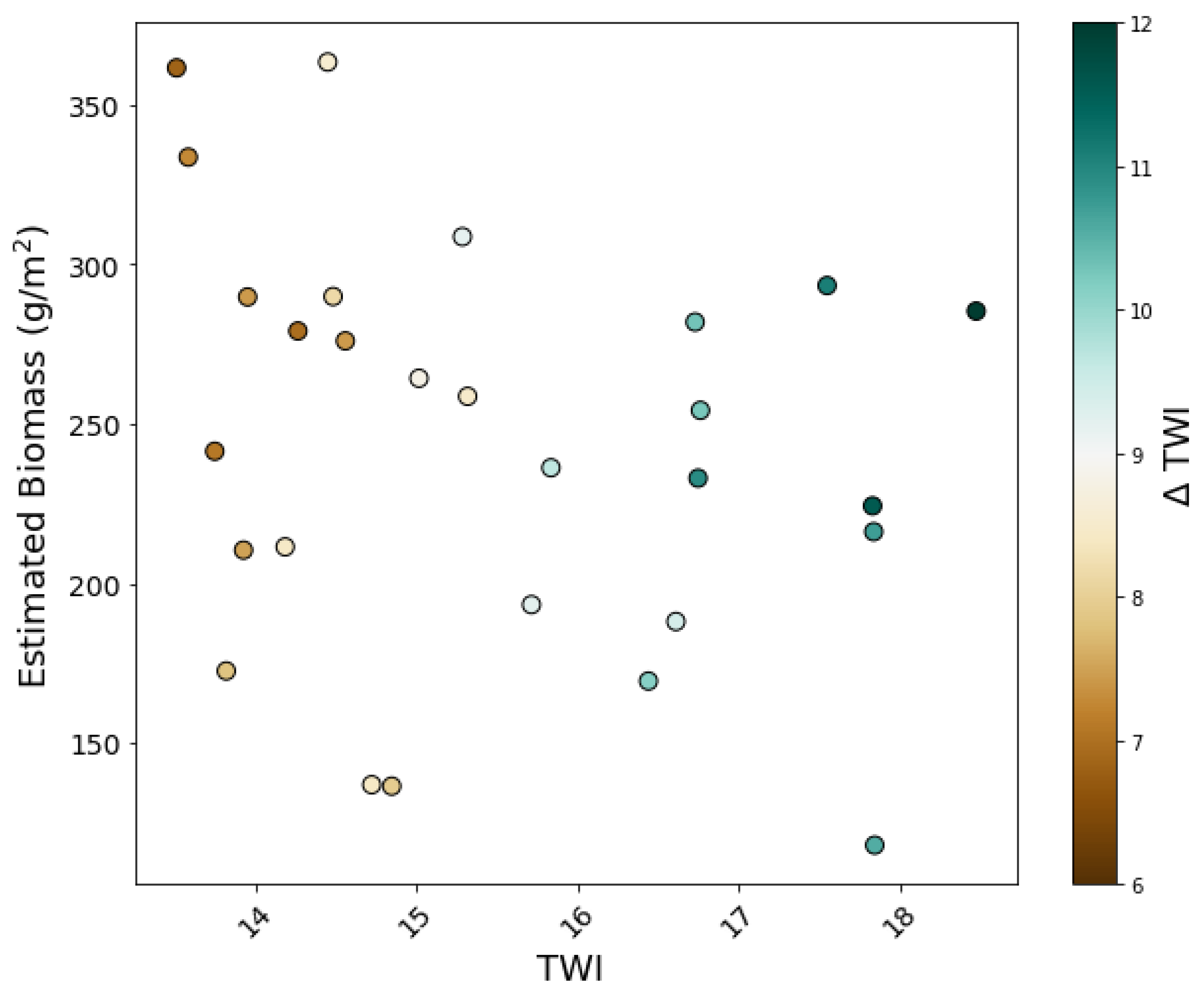
2.4. Identifying Areas of Water Accumulation Using Topographic Wetness Index

Digital terrain analysis is an effective method used in hydrology applications to explore potential variation in water flow and accumulation based on topographic information. Topographic indices reflect the ratio of contributing area to surface slope and so have been used to predict areas of water accumulation [43,44]. The Topographic Wetness Index (TWI) is a function of the natural log of the contributing drainage area per contour length α over the surface slope tan β, as listed in Equation (5) [45].
TWI = ln ( α tan β )
The TWI is calculated from a digital elevation model (DEM). The DEM pixels are used to measure α and tan β. The TWI is used to identify hydrologically similar areas, and in our study to identify areas susceptible to ILA, with TWI calculated from a high-resolution DEM (1.5 m). In the AOI, TWI values range from 2 to 23, where regions of lower values are less susceptible to in-field flooding (Figure 4). As TWI values increase, the susceptibility to soil saturation and in-field flooding increases. The observed extent of inundation measured with the RTK as compared to the TWI is also shown in Figure 4, with an average TWI of 13.5 in the surveyed region. TWI was incorporated into the plot scale analysis by using CIE outputs to extract TWI values for each plot within the defined experiments. Plots extracted with CIE in experiments RUE-1 and RUE-2 are shown as black circles in Figure 4.
In this study, TWI was used to analyze the variation in soybean yield between replicates to explore the potential impact of excess water stress. To analyze the differences, TWI thresholds were applied to identify plots less likely to experience ILA with those that were more likely to experience ILA. Thresholds were determined using spatial analyst in ArcMap 10.5 to calculate average TWI in regions observed to experience inundation, and those observed to be consistently dry. The low TWI threshold was set to 7.4 and the high TWI threshold was set to 13.5. Figure 5 shows a scatter plot comparing soybean yield for all plots under analysis, labeled by class and the plot’s associated TWI value. The red vertical lines indicate the location of the applied thresholds for low and high TWI values. The figure shows that plots with a low TWI value have large range in yield from approximately 2000 kg/ha to 5700 kg/ha, with a median value of 3970 kg/ha. Meanwhile, plots with a high TWI value have less variation in yield, ranging from approximately 2500 kg/ha to 4800 kg ha, and a lower median yield of 3770 kg/ha. Plots located in areas of high TWI were predominantly of the HY and DA classes, while only three plots of the HYD were located in an area of high TWI.
In order to isolate the potential impact of differing wetness conditions, 28 replicate pairs were extracted from the RUE-1 and RUE-2 experiments, in which one plot experienced low TWI (<7.4) and the other experienced high TWI (>13.5). This filtering process allows analysis to focus on replicates that have the potential for different wetness conditions. The replicate plots create opportunities to analyze and compare the soybean development and impact of excess water stress between replicate plots with similar traits. In addition, planting of plots did not take into account TWI, which means that all plots were equally likely to be planted in areas that may or may not experience excess water stress.

3. Results

3.1. Above-Ground Biomass Prediction

Results of the optimization process for each class and expanding all genetic lines are listed in Table 1, which includes the parameter estimates (a, b and c), percent bias (PBIAS) and root mean square error (RMSE). The estimated parameters used to estimate biomass for each class and all classes were similar, with the HYD having the most contrast from accompanying classes listed in Table 1, highlighting the subtle differences in estimated parameters for different genetics. HYD has the lowest PBIAS and RMSE amongst all classes at <0.1% and 64 g/m2, respectively. The constant stem factor (3.50) was also evaluated versus the adjustable stem factor. Overall, the constant stem factor results are very similar to the adjustable stem factor, with a PBIAS and RMSE ranging from −0.5% to −0.6% and 63 g/m2 to 75 g/m2, respectively. Figure 6 compares estimated biomass (g/m2) with respect to measured biomass (g/m2) for classes HY, HYD, DA and all classes from RUE-1. The red line is a 1:1 reference for each comparison to show overestimation or underestimation of estimated biomass with measured biomass. For each class and all classes in RUE-1, RMSE and PBIAS ranged from 64 g/m2 to 73 g/m2 and <0.1% to 0.8%, respectively. The low PBIAS and RMSE for all classes in RUE-1 confirmed that the parameters were representative for all classes under analysis, and it is not necessary to develop equations for each class separately. Figure 6a,d compare the estimated biomass and measured biomass for the HY class and all classes. The equation for all classes was able to accurately represent the range of estimated biomass similar to the dominant class that had 191 plots.
The parameters for each class and for all classes developed from RUE-1 were transferred to RUE-2. Table 1 also lists the PBIAS and RMSE for RUE-2, which ranges from 10.2% to 16.6% and 65 g/m2 to 82 g/m2, respectively. Figure 7 shows subplots comparing estimated biomass (g/m2) with respect to measured biomass (g/m2) for classes HY, HYD, DA and all classes from RUE-2. Overall, the transferred parameters were sufficient at representing the range of estimated biomass for varying genetic classes as well as all classes, as shown in Figure 7. The transferred equation shows slight overestimation of estimated biomass for HY, DA and all classes for RUE-2 displayed in Figure 7a,c,d, respectively. The calculated PBIAS is satisfactory, with all types under analysis below 20% and RMSE comparable to values calculated in RUE-1. The transferred equation shows the ability to accurately estimate biomass for a varying number of plots, such as in the HYD (contains 48 plots) and all classes (contains 377 plots in RUE-2), where the PBIAS is 10.2% and 14.4%, respectively.
Using the representative equation for all classes, above-ground biomass was estimated to analyze the impacts of excess water stress on soybean development. Figure 8 is a spatial map displaying the estimated biomass from a flight date on 17 July 2018 at the R4–R5 stage. In Figure 8, the estimated biomass ranges from 102 g/m2 to 476 g/m2. In RUE-2, the cluster of low biomass values indicated by the red circles correspond with the high TWI values and mapped ILA using the RTK. Additionally, the northeast corner of RUE-1 has low estimated biomass. This section of the field experienced ILA between the R1 and R2 stages of the growing season and corresponds to high TWI values and observed ILA.

3.2. Sensitivity of Above-Ground Biomass to Water Stress

To explore if the estimated above-ground biomass is sensitive to water stress, biomass from plots with observed occurrences of ILA in RUE-2 was compared with biomass from the plot replicate in RUE-1. In-field flooding occurred predominantly in RUE-2, but there was one observation of in-field flooding in RUE-1. In 2018, ILA was observed on June 25th, July 6th and July 12th in RUE-2. The ILA observed on June 25th was also observed in RUE-1 at the R1–R2 stage, from a large rainfall event (32 mm) on June 23rd, demonstrating that ILA can persist for at least two days even with subsurface drains. In addition, heavy cumulative precipitation of 29 mm occurred during critical periods of the reproductive stages (R4–R6). This comparison analysis used the measured and estimated biomass collected on July 16th and 17th, respectively, at the R4–R5 stage and harvested yield from the plot replicates to calculate the percent difference in yield. Figure 9 displays the increase occurrence of inundation for each plot in RUE-2, compared to plots in RUE-1, resulting in a decrease in biomass for each plot in RUE-2. The figure shows that the plots in RUE-2 have lower biomass, on average, than plots in RUE-1, with an average measured and estimated biomass of 140 g/m2 and 160 g/m2, respectively. Conversely, the average measured and estimated biomass for plots in RUE-1 are both 320 g/m2. Figure 9 also highlights that measured and estimated biomass show agreement, with an RMSE of 20 g/m2 and 30 g/m2 for plots analyzed in RUE-1 and RUE-2, respectively. This analysis was completed using plots where ILA had been observed. The comparison of replicate plots revealed noticeable differences from the impacts of excess water stress on measured and estimated biomass at the early growth stages (R4–R5) of soybean and demonstrates that Equation (2) is sensitive to the impacts of excess water stress.
To assess the effects of excess water stress on biomass, an objective approach is needed to distinguish between plots that are more susceptible to ILA and plots that are less susceptible to ILA and recognize that soybean can be impacted by excess soil moisture conditions even before surface ponding is visible. The TWI can be used to distinguish plots using TWI thresholds with the estimated biomass. Replicate plots in areas of high TWI were analyzed and compared with plots in low TWI to quantify the effects of excess water stress on biomass. TWI thresholds of 7.4 and 13.5 were used for low and high areas of TWI, respectively. The change in TWI (∆TWI) between replicate plots was also evaluated by taking the difference between plots in areas of high TWI minus low TWI. Biomass was estimated using Equation (2) with parameters representing all classes in RUE-1 and RUE-2. A total of 28 replicate plots were identified that were located in areas of high susceptibly to excess water stress with a reference replicate in an area less susceptible to excess water stress.
The relationship between estimated biomass and TWI for the replicate plots in areas of high TWI at early growth stages (R4–R5) is analyzed in Figure 10. Estimated biomass and TWI range from approximately 120 g/m2 to 360 g/m2 and 13.5 to 18.5, respectively. In general, plots located in areas of increasing TWI (>15) are more susceptible to excess water stress and have a decrease in estimated biomass. Figure 10 also shows that as the ∆TWI between high and low TWI replicates increases more than 9, plots with a reduced biomass are located in areas more susceptible to excess water stress.

3.3. Quantifying the Impacts of Excess Water Stress on Yield

It has been established that biomass from the R4–R5 stage is sensitive to differences in wetness conditions, and that the fitted model is able to capture these differences. The next step is to translate these early season differences into differences in yield due to excess water stress alone. Figure 9 shows that the decreased biomass at the R4–R5 stage from plots experiencing ILA in RUE-2 also resulted in a decrease in yield ranging from approximately 5% to 18%, relative to the RUE-1 replicate. In most cases, the change in yield correlates with the change in biomass. Interestingly, the exception to this relationship is for a pair of replicate plots that both experienced occurrences of ILA, where in-field flooding had been observed once in RUE-1 and three times in RUE-2 (Figure 9). The measured and estimated biomass for the plots is relatively low compared to other plots, where the biomass is no more than 130 g/m2 at the R4–R5 stage. The decline in yield for RUE-2 relative to RUE-1, however, is approximately 15%. This implies that the RUE-1 plot actually recovered better from exposure to a single ILA occurrence, relative to the RUE-2 plot, which had three occurrences of ILA.
The percent of expected yield was estimated based on observations from the early growth stages (R4–R5), using Equation (4), to quantify and identify yield impacts from excess water stress for stakeholders. Figure 11 demonstrates the relationship between the percent of expected yield and relative biomass at R4–R5 for plots in areas of high TWI. The range of percent of expected yield is from 52% to 151%, while the range of relative biomass is 0.41 to 1.25. Figure 11 demonstrates the linear model (Equation (4)), which shows a positive linear correlation. The correlation across all plots is not significant, with a correlation coefficient (r) of 0.32. The F-statistic of the regression is not significant at 0.05 but is significant at 0.1. In general, as relative biomass increased, ∆estimated biomass also increased, which transitioned to a positive increase in percent of expected yield.
Figure 12 demonstrates how this model can be used to map potential yield loss due specifically to excess water stress across a field or experiment. The range of percent of expected yield is from 83% to 125%. The average percent of expected yield is 103%. The lowest values of percent of expected yield between 83% and 90% occur predominately in areas susceptible to inundation. For RUE-1, plots with the lowest percent of expected yield occur in the northeast corner, which corresponds to the high TWI and mapped ILA. In RUE-2, plots with the lowest percent of expected yield occur towards the center of the field and also correspond with high TWI and mapped ILA. In RUE-1, the percent of expected yield generally increases in the direction from east to west. In RUE-2, the percent of expected yield generally increases from west to east.

4. Discussion

4.1. UAS Data Processing Pipeline

A data processing pipeline was developed for high-throughput phenotyping at the plot level with CIE and VID [31]. The developed tools enabled calibration and plant phenotyping at the plot scale for multiple flight dates to estimate potential yield loss by excess water stress. This form of data processing can be time- and data-intensive, as indicated by Shi et al. [45]. In their study, 38,000 plots were manually extracted from orthomosaics [46]. Creating automated tools to extract plot images, calibrate images and apply band algorithms can be additional challenges that limit the time needed to answer primary objective science questions. CIE and VID are Python tools that were developed to reduce the aforementioned burden and place more time and focus on the science questions. Shi et al. [46] and Maimaitijiang et al. [7] have used orthomosaics for plant phenotyping of soybean generated from stitched images with RGB, multispectral and thermal sensors on UAS platforms. In this study, orthomosaics were also used for estimating biomass from multispectral stitched images. CIE now has the capability to extract plots from the original images from RGB, multispectral and thermal imagery, which can generate multiple replicate plot images within an experiment. Future research should analyze the original images and test data fusion and/or deep learning to predict yield.

4.2. Predicting Above-Ground Biomass

Expanding the methodology developed from Jackson et al. [37] and Chan et al. [40] for estimation of VWC to estimate above-ground biomass for different soybean classes (HY, HYD and DA) and across all classes proved to be representative and transferable. The incorporated adjustable stem water content variable provided only minor improvements when compared to the constant stem factor. This finding provides insight that the estimated biomass was not significantly influenced by the adjustable stem factor. Parameters used to estimate biomass representing all genetic classes within RUE-1 had low PBIAS and satisfactory RMSE. The equation used for all classes in RUE-1 was transferred to RUE-2 to estimate biomass for all plots. Estimated biomass in RUE-2 had satisfactory PBIAS and RMSE but was generally overestimated when compared with in-situ data. The overestimation in RUE-2 is attributed to biomass values (and associated parameters) from RUE-1 being generally higher than biomass in RUE-2, which caused estimated values in RUE-2 to have a positive bias. The soybean plots in RUE-1 had less occurrences of inundation, with an average biomass and yield of 278 g/m2 and 4150 kg/ha, respectively. Comparatively, RUE-2 had more occurrences of ILA and lower average biomass and yield of approximately 263 g/m2 and 3680 kg/ha, respectively. The positive bias suggests that the biomass algorithm is potentially less sensitive to excess water stress and may reduce the significance of Equation (4). Representative variability in estimated biomass was observed in RUE-1 and RUE-2, where low values corresponded with mapped ILA. The transferability demonstrates the potential use in future research to develop models within a defined experiment and scale-up the model across multiple fields for plant phenotyping.
In our study, models were generated to estimate above-ground biomass at the R4–R5 stage using a flight one day after sampling. Zhang et al. [47] used UASs to analyze soybean yield prediction models that incorporated measurements from one or two growth stages. They found that the R5 stage was the best growth stage for the single-stage model, and the R4 and R5 stages were the best combination of stages for the two-growth-stage model. The close interval between in-situ sampling and remotely sensed observation was an important factor for estimating adequate parameters to estimate biomass. Using the developed models for different development stages does introduce uncertainty. This could not be tested since in-situ biomass data were only collected at the R4–R5 stage to protect the integrity of the experiment. To build and validate representative models to predict biomass, dense in-situ sampling to capture variability at important development stages with corresponding flight dates should be considered. Previous studies have shown the blooming to seed filling stages (R2–R5) to be critical for soybean yield prediction [5,7,18].

4.3. Quantifying Impacts of Excess Water Stress on Yield

Proximal remote sensing with digital terrain analysis was used to detect and estimate potential gross yield loss from excess water stress at the plot scale. The calculated and mapped TWI agreed with in-situ observations of ILA. TWI alone was not strongly correlated with percent difference in yield. TWI was measured at 1.5 m resolution, which highlighted the in-field variability of TWI. The TWI thresholds were used to provide an objective approach to distinguish inundation susceptibility between replicate plots. However, some plots that did experience flooding did not meet the threshold criteria and as a result were not used in the comparison analysis. This study also showed that plots located in areas of high TWI (>13.5) can have higher yields than plots located in areas of low TWI (<7.4) if the occurrence of ILA is limited and providing optimal soil moisture conditions for the soybean to thrive. For instance, plots in RUE-1 had less observed occurrences of ILA than plots in RUE-2, and as a result, some plots developed in areas of high TWI had a higher yield than plots in RUE-2 located in areas of low TWI. For future studies, soil moisture and inundation duration should be considered when mapping regions that experienced inundation. Previous work used remotely sensed observations of soil moisture to identify flooded areas in croplands from Soil Moisture Active Passive (SMAP). Though SMAP observations are at a coarser resolution than what is needed for this study, the results demonstrated the potential of soil moisture to identify areas susceptible to inundation in cropland areas [48]. Paul et al. [49] used remotely sensed observations to measure the duration of inundation in corn and soybean. Observations of duration and intensity of inundation could provide better insight into the effects of excess water stress on crop yield.
Using TWI to identify plots with contrasting wetness potential improved the detection and estimation of yield loss caused by excess water stress. By comparing and evaluating plots impacted by ILA with replicate plots not impacted by ILA, distinguishable differences in estimated biomass were identified in the early growth stages (R4–R5), which correspond to the results of previous studies. In-situ experiments from Desmond et al. [4] and Scott et al. [50] calculated crop susceptibility factors for flood duration effects on indeterminate and determinate soybean, respectively. Results of their studies found agreement that the indeterminate and determinate soybean were most susceptible to flooding during early growth stages.
Mapping the percent of expected yield with CIE provided the ability to evaluate the soybeans spatially at the R4–R5 stage. By integrating mapped ILA observations with digital terrain analysis from TWI, inferences relating to potential yield reduction due to excess water stress could be made with supportive data. Similar data fusion frameworks would be useful for stakeholders and provide the information needed to make management decisions.

5. Conclusions

Low-gradient agricultural areas often experience ILA in the Midwest, resulting in damaged crops and increased financial risk from yield loss. By identifying areas impacted by excess water stress early in the reproductive stages, stakeholders can assess risk and make investment plans for responsive management decisions. The potential of low-cost UASs to measure impacts of excess water stress on soybean development were analyzed and evaluated along with new tools, CIE and VID, designed to help with the extraction of plots within breeding experiments. The aims of this study were to address the questions (1) Can proximal remote sensing be used to detect excess water stress in soybean? and (2) What is the potential yield effect from ILA? The main conclusions of the investigation are:
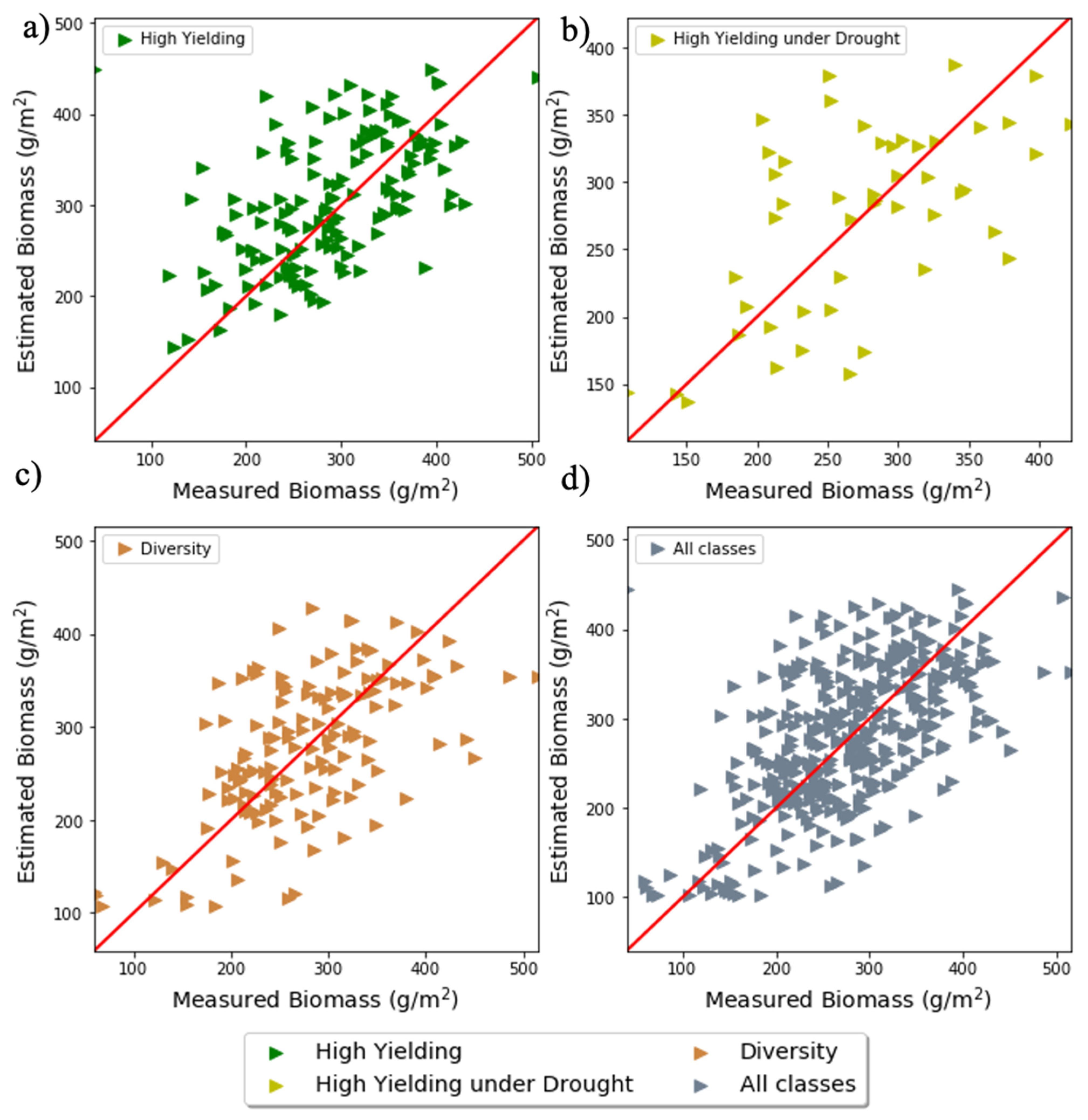
  • Proximal remote sensing from UASs is a representative predictor of biomass at the R4–R5 stage at the plot scale. Expanding the methodology developed from Jackson et al. [37] and Chan et al. [40] for the estimation of VWC to estimate biomass proved to be representative and transferable. Soybean of varying classes (HY, HYD and DA) was analyzed and a representative estimate of biomass for all genetic lines was generated.
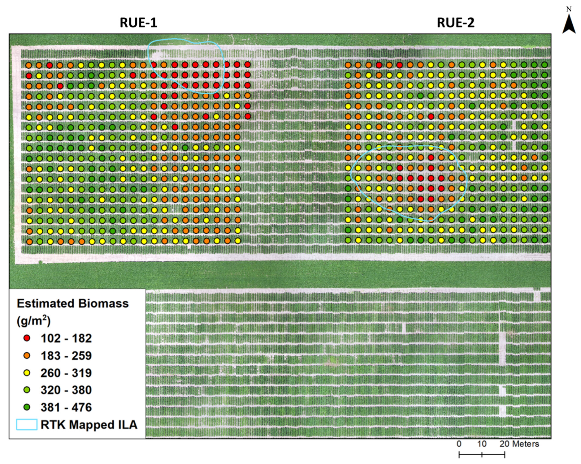
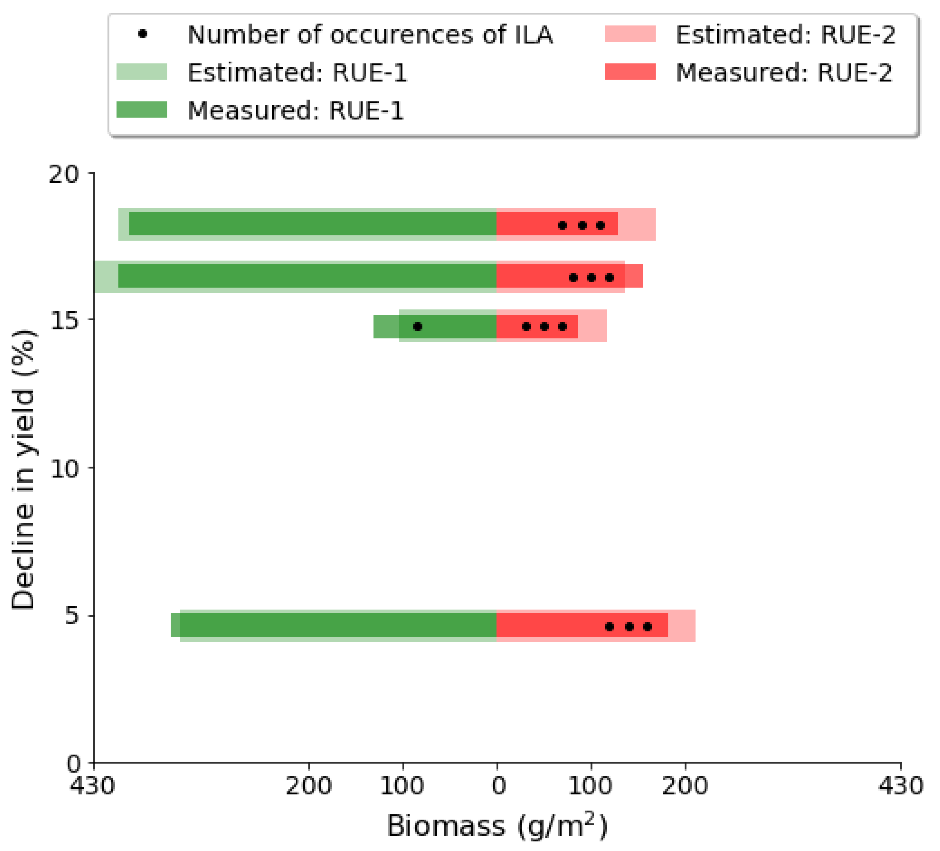
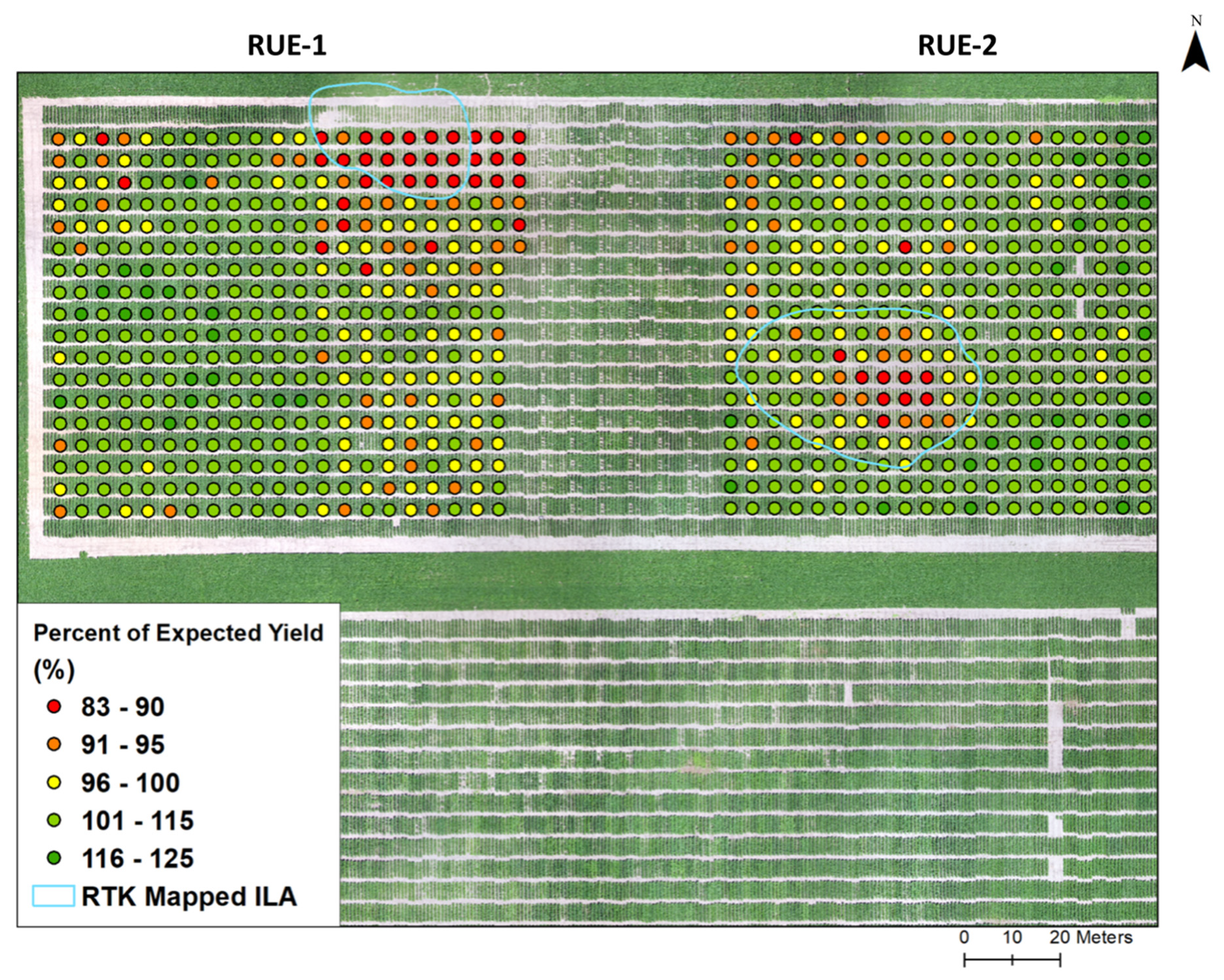
  • Estimated biomass at early growth stages (R4–R5) proved to be sensitive to excess water stress, though it was less sensitive than the in-situ biomass. The sensitivity of estimated biomass to excess water stress was analyzed and evaluated at the plot and field scale. The sensitivity of estimated biomass sensitivity to excess water stress was distinguishable in the early growth stages. Concentrated areas of low estimates of biomass showed agreement with mapped ILA and areas of high TWI.
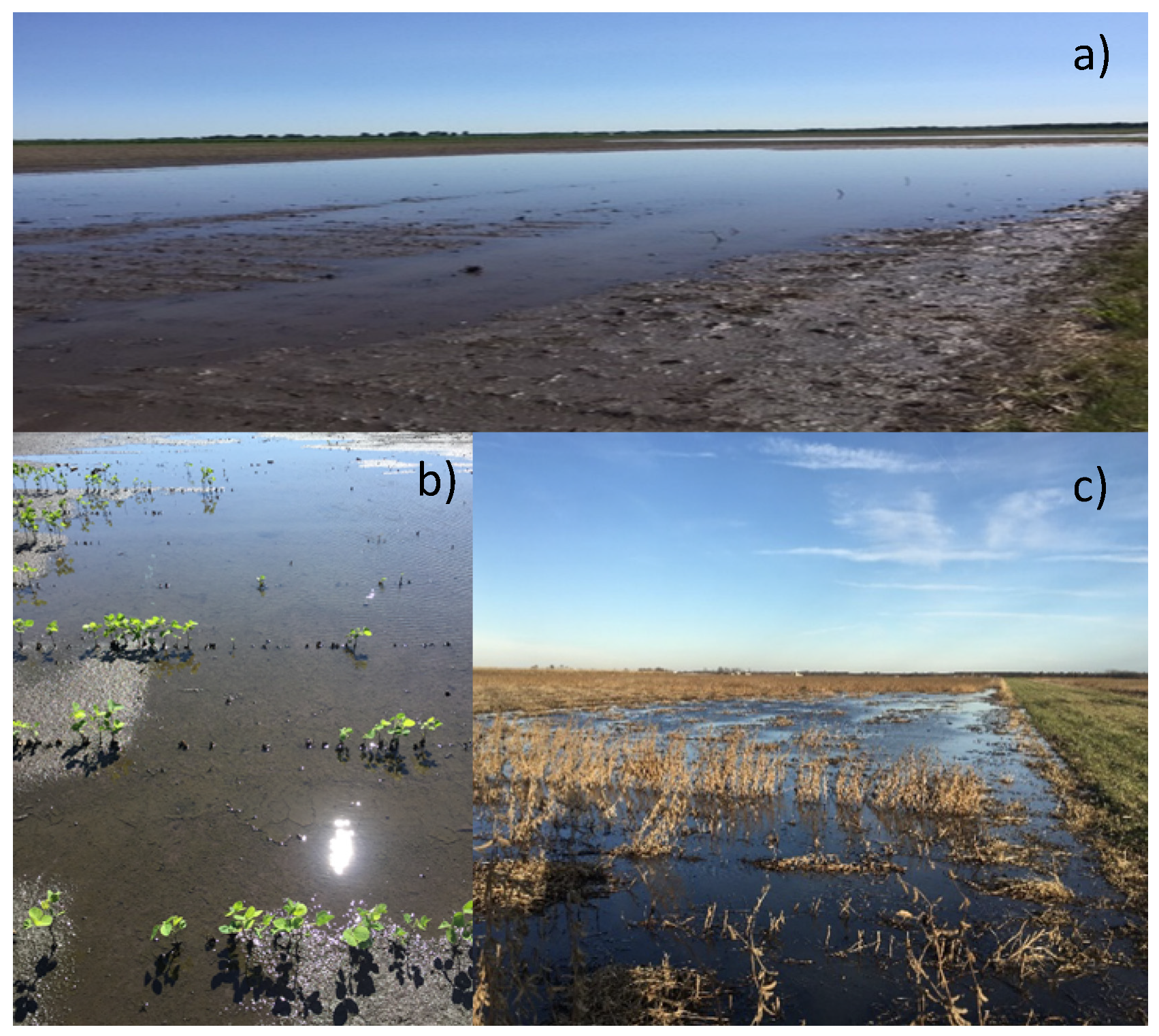
  • Low estimates of the percent of expected yield corresponded with observations of in-field flooding and areas with high TWI, whereas high estimates of the percent of expected yield corresponded with areas less susceptible to inundation. Estimates of potential yield reduction mapped with developed tools provide a useful crop status assessment at the R4–R5 stage.
The results of this study demonstrate transferable methods to estimate early-season biomass at the plot scale and potential yield loss due to excess water stress, which provide crop status assessments to stakeholders prior to harvest. Future improvements of the current method should aim to better directly incorporate measurements of the intensity and duration of excess water stress. To improve the quantification of inundation, future studies should incorporate observations of soil moisture and use geospatial models as necessary to determine the spatial distribution of saturation. In addition, the duration of inundation can be estimated using observed water table data or remotely sensed observations from the UAS. Future work will aim to (1) leverage high-resolution satellite data to fill data gaps and analyze the effect of excess water stress on estimated biomass at larger scales and (2) incorporate land surface model simulations to estimate the potential yield reduction from excess water stress at varying scales.

Author Contributions

Conceptualization, S.D.S., L.C.B. and K.A.C.; methodology, S.D.S., L.C.B. and K.A.C.; writing—review and editing, S.D.S., L.C.B., K.A.C. and K.M.R.; funding acquisition, K.A.C., K.M.R. All authors have read and agreed to the published version of the manuscript.

Funding

This research was funded by the United States Department of Agriculture, grant number 2016-07982.

Conflicts of Interest

The authors declare no conflict of interest.

References

  1. Pack, D.J. About $300 Million in INDIANA Crops’ Value Lost to Flooding So Far; Purdue Extension: West Lafayette, IN, USA, 2015; Available online: https://extension.purdue.edu/Parke/pages/article.aspx?intItemID=10734 (accessed on 16 May 2018).
  2. DeBoer, D.W.; Ritter, W.F. Flood Damage to Crops in Depression Areas of North-Central Iowa. Trans. ASAE 1970, 13, 0547–0549. [Google Scholar] [CrossRef]
  3. Evans, R.O.; Fausey, N.R. Effects of Inadequate Drainage on Crop Growth and Yield. Agron. Monogr. Agron. 2015, 13–54. [Google Scholar] [CrossRef]
  4. Desmond, E.D.; Barkle, G.F.; Schwab, G.O. Soybean yield response to excess water. Am. Soc. Agric. Eng. (Microfiche Collect.) (USA) 1985, 1–12. [Google Scholar]
  5. Gao, F.; Anderson, M.; Daughtry, C.; Johnson, D. Assessing the Variability of Corn and Soybean Yields in Central Iowa Using High Spatiotemporal Resolution Multi-Satellite Imagery. Remote Sens. 2018, 10, 1489. [Google Scholar] [CrossRef] [Green Version]
  6. Wiegand, C.L.; Richardson, A.J.; Jackson, R.D.; Pinter, P.J.; Aase, J.K.; Smika, D.E.; Lautenschlager, L.F.; McMurtrey, J. Development of agrometeorological crop model inputs from remotely sensed information. IEEE Trans. Geosci. Remote Sens. 1986, 90–98. [Google Scholar] [CrossRef]
  7. Maimaitijiang, M.; Sagan, V.; Sidike, P.; Hartling, S.; Esposito, F.; Fritschi, F.B. Soybean yield prediction from UAV using multimodal data fusion and deep learning. Remote Sens. Environ. 2020, 237, 111599. [Google Scholar] [CrossRef]
  8. Iowa State University. How a Soybean Plant Develops. 1985. Available online: http://publications.iowa.gov/14855/ (accessed on 2 May 2018).
  9. Fehr, W.R.; Caviness, C.E.; Burmood, D.T.; Pennington, J.S. Stage of Development Descriptions for Soybeans, Glycine max (L.) Merrill 1. Crop. Sci. 1971, 11, 929–931. [Google Scholar] [CrossRef]
  10. Griffin, J.L.; Saxton, A.M. Response of Solid-Seeded Soybean to Flood Irrigation. II. Flood Duration. Agron. J. 1988, 80, 885–888. [Google Scholar] [CrossRef]
  11. Enquist, B.J. Global Allocation Rules for Patterns of Biomass Partitioning in Seed Plants. Science 2002, 295, 1517–1520. [Google Scholar] [CrossRef] [Green Version]
  12. Niklas, K.J.; Enquist, B.J. Canonical rules for plant organ biomass partitioning and annual allocation. Am. J. Bot. 2002, 89, 812–819. [Google Scholar] [CrossRef] [Green Version]
  13. Hunt, E.R.; Li, L.; Yilmaz, M.T.; Jackson, T.J. Comparison of vegetation water contents derived from shortwave-infrared and passive-microwave sensors over central Iowa. Remote Sens. Environ. 2011, 115, 2376–2383. [Google Scholar] [CrossRef]
  14. Monteith, J.L. Climate and the efficiency of crop production in Britain. Philos. Trans. R. Soc. Lond. B 1977, 281, 277–294. [Google Scholar] [CrossRef]
  15. Lobell, D.B.; Asner, G.; Ortiz-Monasterio, J.; Benning, T.L. Remote sensing of regional crop production in the Yaqui Valley, Mexico: Estimates and uncertainties. Agric. Ecosyst. Environ. 2003, 94, 205–220. [Google Scholar] [CrossRef] [Green Version]
  16. Lobell, D. The use of satellite data for crop yield gap analysis. Field Crop. Res. 2013, 143, 56–64. [Google Scholar] [CrossRef] [Green Version]
  17. Wang, R.; Cherkauer, K.; Bowling, L. Corn Response to Climate Stress Detected with Satellite-Based NDVI Time Series. Remote Sens. 2016, 8, 269. [Google Scholar] [CrossRef] [Green Version]
  18. Ma, B.L.; Dwyer, L.M.; Costa, C.; Cober, E.; Morrison, M.J. Early Prediction of Soybean Yield from Canopy Reflectance Measurements. Agron. J. 2001, 93, 1227–1234. [Google Scholar] [CrossRef] [Green Version]
  19. Jones, H.G.; Vaughan, R.A. Remote Sensing of Vegetation: Principles, Techniques, and Applications; Oxford University Press: Oxford, UK, 2010. [Google Scholar]
  20. Kross, A.; McNairn, H.; Lapen, D.; Sunohara, M.; Champagne, C. Assessment of RapidEye vegetation indices for estimation of leaf area index and biomass in corn and soybean crops. Int. J. Appl. Earth Obs. Geoinf. 2015, 34, 235–248. [Google Scholar] [CrossRef] [Green Version]
  21. Chen, D.; Huang, J.; Jackson, T.J. Vegetation water content estimation for corn and soybeans using spectral indices derived from MODIS near- and short-wave infrared bands. Remote Sens. Environ. 2005, 98, 225–236. [Google Scholar] [CrossRef]
  22. Johnson, D.M. An assessment of pre- and within-season remotely sensed variables for forecasting corn and soybean yields in the United States. Remote Sens. Environ. 2014, 141, 116–128. [Google Scholar] [CrossRef]
  23. Yilmaz, M.T.; Hunt, E.R.; Jackson, T.J. Remote sensing of vegetation water content from equivalent water thickness using satellite imagery. Remote Sens. Environ. 2008, 112, 2514–2522. [Google Scholar] [CrossRef]
  24. Zhang, C.; Kovacs, J.M. The application of small unmanned aerial systems for precision agriculture: A review. Precis. Agric. 2012, 13, 693–712. [Google Scholar] [CrossRef]
  25. Widhalm, M.; Hamlet AByun, K.; Robeson, S.; Baldwin, M.; Staten, P.; Chiu, C.; Coleman, J.; Hall, E.; Hoogewind, K.; Huber, M.; et al. Indiana’s Past & Future Climate: A Report from the Indiana Climate Change Impacts Assessment; Purdue Climate Change Research Center, Purdue University: West Lafayette, IN, USA, 2018. [Google Scholar] [CrossRef] [Green Version]
  26. Alberto, B.; District, S.P.; Banitt, A.; Faber, B. Red River of the North at Fargo, North Dakota, Pilot Study, Impact of Climate Change on Flood Frequency Curve. 2015. Available online: https://usace.contentdm.oclc.org/utils/getfile/collection/p266001coll1/id/6725 (accessed on 1 May 2018).
  27. Farm Production and Conservation Business Center. Report: Farmers Prevented from Planting Crops on More than 19 Million Acres; U.S. Department of Agriculture Farm Service Agency: Washington, DC, USA, 2019. Available online: https://www.fsa.usda.gov/news-room/news-releases/2019/report-farmers-prevented-from-planting-crops-on-more-than-19-million-acres (accessed on 12 August 2019).
  28. Soil Survey Staff, Natural Resources Conservation Service, United States Department of Agriculture. Web Soil Survey. Available online: https://websoilsurvey.sc.egov.usda.gov/ (accessed on 20 March 2018).
  29. Song, Q.; Yan, L.; Quigley, C.; Jordan, B.D.; Fickus, E.; Schroeder, S.; Song, B.; An, Y.C.; Hyten, D.; Nelson, R.; et al. Genetic Characterization of the Soybean Nested Association Mapping Population. Plant. Genome 2017, 10. [Google Scholar] [CrossRef] [Green Version]
  30. Smith, G.M.; Milton, E.J. The use of the empirical line method to calibrate remotely sensed data to reflectance. Int. J. Remote Sens. 1999, 20, 2653–2662. [Google Scholar] [CrossRef]
  31. Lyu, B.; Smith, S.D.; Xue, Y.; Rainey, K.M.; Cherkauer, K. An Efficient Pipeline for Crop Image Extraction and Vegetation Index Derivation Using Unmanned Aerial Systems. Trans. ASABE 2020, 63, 1133–1146. [Google Scholar] [CrossRef]
  32. Hearst, A.A.; Cherkauer, K.A. Research Article: Extraction of Small Spatial Plots from Geo-Registered UAS Imagery of Crop Fields. Environ. Pract. 2015, 17, 178–187. [Google Scholar] [CrossRef]
  33. Pix4D; Pix4D SA: Lausanne, Switzerland, 2018; Available online: https://www.pix4d.com/ (accessed on 6 July 2021).
  34. Monteith, J.L. Solar Radiation and Productivity in Tropical Ecosystems. J. Appl. Ecol. 1972, 9, 747–766. [Google Scholar] [CrossRef] [Green Version]
  35. Liu, J.; Pattey, E.; Miller, J.R.; McNairn, H.; Smith, A.; Hu, B. Estimating crop stresses, aboveground dry biomass and yield of corn using multi-temporal optical data combined with a radiation use efficiency model. Remote Sens. Environ. 2010, 114, 1167–1177. [Google Scholar] [CrossRef]
  36. Gao, B.-C.; Goetzt, A.F. Retrieval of equivalent water thickness and information related to biochemical components of vegetation canopies from AVIRIS data. Remote Sens. Environ. 1995, 52, 155–162. [Google Scholar] [CrossRef]
  37. Kim, Y.; Jackson, T.; Bindlish, R.; Lee, H.; Hong, S. Radar Vegetation Index for Estimating the Vegetation Water Content of Rice and Soybean. IEEE Geosci. Remote Sens. Lett. 2012, 9, 564–568. [Google Scholar] [CrossRef]
  38. Jackson, T.; Le Vine, D.; Hsu, A.; Oldak, A.; Starks, P.; Swift, C.; Isham, J.; Haken, M. Soil moisture mapping at regional scales using microwave radiometry: The Southern Great Plains Hydrology Experiment. IEEE Trans. Geosci. Remote Sens. 1999, 37, 2136–2151. [Google Scholar] [CrossRef] [Green Version]
  39. Jackson, T.; Schmugge, T. Vegetation effects on the microwave emission of soils. Remote Sens. Environ. 1991, 36, 203–212. [Google Scholar] [CrossRef]
  40. Lawrence, H.; Wigneron, J.-P.; Richaume, P.; Novello, N.; Grant, J.; Mialon, A.; Al Bitar, A.; Merlin, O.; Guyon, D.; Leroux, D.; et al. Comparison between SMOS Vegetation Optical Depth products and MODIS vegetation indices over crop zones of the USA. Remote Sens. Environ. 2014, 140, 396–406. [Google Scholar] [CrossRef]
  41. Chan, S.; Bindlish, R.; Hunt, R.; Jackson, T.; Kimball, J. Ancillary Data Report: Vegetation Water Content. No. SMAP Science Document 047. 2013; pp. 1–15. Available online: Smap.jpl.nasa.gov (accessed on 3 March 2018).
  42. Zhang, J.; Xu, Y.; Yao, F.; Wang, P.; Guo, W.; Li, L.; Yang, L. Advances in estimation methods of vegetation water content based on optical remote sensing techniques. Sci. China Ser. E Technol. Sci. 2010, 53, 1159–1167. [Google Scholar] [CrossRef]
  43. Quinn, P.F.; Beven, K.J.; Lamb, R. The ln(a/tan Beta) Index: How to Use It Within the TOPMODEL Framework. Hydrol. Process. 1995, 9, 161–182. [Google Scholar] [CrossRef]
  44. Grimm, K.; Nasab, M.T.; Chu, X. TWI Computations and Topographic Analysis of Depression-Dominated Surfaces. Water 2018, 10, 663. [Google Scholar] [CrossRef] [Green Version]
  45. Beven, K.J.; Kirkby, M.J. A physically based, variable contributing area model of basin hydrology/Un modèle à base physique de zone d’appel variable de l’hydrologie du bassin versant. Hydrol. Sci. J. 1979, 24, 43–69. [Google Scholar] [CrossRef] [Green Version]
  46. Shi, Y.; Thomasson, J.A.; Murray, S.C.; Pugh, N.A.; Rooney, W.L.; Shafian, S.; Rajan, N.; Rouze, G.; Morgan, C.L.; Neely, H.L.; et al. Data from: Unmanned aerial vehicles for high-throughput phenotyping and agronomic research. PLoS ONE 2016, 11, 1–26. [Google Scholar] [CrossRef] [Green Version]
  47. Zhang, X.; Zhao, J.; Yang, G.; Liu, J.; Cao, J.; Li, C.; Zhao, X.; Gai, J. Establishment of Plot-Yield Prediction Models in Soybean Breeding Programs Using UAV-Based Hyperspectral Remote Sensing. Remote Sens. 2019, 11, 2752. [Google Scholar] [CrossRef] [Green Version]
  48. Rahman, S.; Di, L.; Yu, E.; Lin, L.; Zhang, C.; Tang, J. Rapid Flood Progress Monitoring in Cropland with NASA SMAP. Remote Sens. 2019, 11, 191. [Google Scholar] [CrossRef] [Green Version]
  49. Paul, R.F.; Cai, Y.; Peng, B.; Yang, W.H.; Guan, K.; DeLucia, E.H. Spatiotemporal Derivation of Intermittent Ponding in a Maize–Soybean Landscape from Planet Labs CubeSat Images. Remote Sens. 2020, 12, 1942. [Google Scholar] [CrossRef]
  50. Scott, H.D.; DeAngulo, J.; Daniels, M.B.; Wood, L.S. Flood Duration Effects on Soybean Growth and Yield. Agron. J. 1989, 81, 631–636. [Google Scholar] [CrossRef]
Figure 1. Image of inundated land area during different development stages of soybean in an agricultural field in West–Central Indiana: (a) extent and shallow depth of ILA after planting, (b) vegetative stage where the impacts of ILA prevented some plants from developing leaves, and (c) reproductive stage where the impacts of ILA have caused lodging in some plants.
Remotesensing 13 02911 g001
Figure 2. Map view of the field experiment, located in West–Central IN. Two areas of interests were analyzed, which are outlined in black and blue. The black outline represents the area of experiment 1, RUE-1. The blue outline is the second experiment, RUE-2. The extent of inundation was mapped using TOPCON Real Time Kinematic (RTK) surveying equipment. Ground control points were used to define extent of experiments.
Remotesensing 13 02911 g002
Figure 3. Illustration of components of a defined experiment from Crop Image Extraction and Vegetation Indices Derivation. The user has defined an experiment made of four crop rows and two crop ranges, and each crop plot contains six crop units. The experiment is made up of four crop rows and two crop ranges. CIE extracts replicate plot images from the UAS during a flight over an area of interest. CIE enables the user to define an experiment, and the tool then highlights the canopy, grids the experiment and extracts the replicate plot images from each gridded plot. VID is used to calibrate images and compute vegetation indices of interest.
Remotesensing 13 02911 g003
Figure 4. Map of Topographic Wetness Index (TWI) calculated from a 1.5 m resolution DEM at the study location. Lower values shown in brown are less suspectable to in-field flooding. The transition from brown to blue shows an increase in susceptibility of in-field flooding. Mapped inundated land area (ILA) shows agreement with the calculated TWI. Crop Image Extraction (CIE) can be used to extract TWI from plots within a defined experiment. The black circles represent the extracted plots from RUE-1 and RUE-2.
Remotesensing 13 02911 g004
Figure 5. Scatter plot of the relationship between Topographic Wetness Index (TWI) and soybean yield (kg/ha) labeled by class. TWI thresholds at 7.4 and 13.5 were set to compare RUE-1 and RUE-2 replicates less likely to experience ILA to those that were more likely to experience ILA. The low and high TWI ranges used in analysis are represented by arrows.
Remotesensing 13 02911 g005
Figure 6. Scatter plots comparing estimated biomass with measured biomass at the R4–R5 development stage for each class and all classes in RUE-1 shown as triangles. (a) High Yielding, (b) High Yielding under Drought, (c) Diversity and (d) all classes. Parameters were estimated for each class to consider varying soybean genetics and for all classes to determine if one set of parameters could be representative for all classes.
Remotesensing 13 02911 g006
Figure 7. Scatter plots comparing estimated biomass with measured biomass at the R4–R5 development stage for each class and classes in RUE-2 shown as circles. (a) High Yielding, (b) High Yielding under Drought, (c) Diversity and (d) all classes. Parameters were transferred from RUE-1 to RUE-2.
Remotesensing 13 02911 g007
Figure 8. Estimated biomass (g/m2) of soybean on 17 July 2018 at early growth stages (R4–R5) for experiments in RUE-1 and RUE-2. Outputs generated using CIE and VID. Plots of low estimated biomass values are shown in red and the transition to green represents an increase in estimated biomass. Plots with low estimated biomass correspond with mapped inundated land area.
Remotesensing 13 02911 g008
Figure 9. Four pairs of replicate plots in RUE-1 and RUE-2 analyzing the effects of excess water stress on the percent difference in yield with respect to the measured and estimated biomass (g/m2) at the R4–R5 stage. Increasing biomass estimate for RUE-1 is plotted to the left, for RUE-2 to the right, with zero biomass in the center of the plot. Decline in yield, reported as a percent difference between RUE-2 and RUE-1, is indicated by vertical position of the bar relative to the RUE-1 replicate. Black circles indicate each observed occurrence of inundated land area for the plot. The biomass was sampled on 16 July 2018 and remotely sensed estimates of biomass were made on 17 July.
Remotesensing 13 02911 g009
Figure 10. Analyzing the interactions between estimated biomass, TWI and ∆ TWI at the early growth stage (R4–R5). Values are colored with the difference in TWI between replicate plots, which ranges from 7 to 12.
Remotesensing 13 02911 g010
Figure 11. Comparing interactions between percent of expected yield (%) with respect to relative biomass (fraction) and the ∆ estimated biomass (g/m2) at the early growth stage (R4–R5).
Remotesensing 13 02911 g011
Figure 12. Percent of expected yield (%) from 17 July 2018 at the R4–R5 stage. Values below 90% (red to orange) indicate areas predicted more likely to have a lower yield, whereas values greater than 95% (yellow to green) predict a higher estimate of yield.
Remotesensing 13 02911 g012
Table 1. Estimated parameters for High Yielding (HY), High Yielding under Drought (HYD), Diversity (DA) and all classes for RUE-1 and RUE-2 with calculated percent bias (PIBAS) and root mean square error (RMSE). Parameters from RUE-1 were transferred to RUE-2. The constant stem factor was also analyzed to compare with the adjustable stem factor.
Type and Number of PlotsParameter aParameter bParameter cPBIAS (%)RMSE (g/m2)
RUE-1
HY
191 plots
1817.06−1022.2226.90.873
HYD
48 plots
2382.77−1863.25497.97<0.164
DA
144 plots
1993.46−1267.85308.15<0.170
All classes
383 plots
1955.75−1217.37290.230.872
HY—constant stem factor
191 plots
464.06761.75−372.22−0.675
HYD—constant stem factor
48 plots
2379.15−1856.73493−0.563
DA—constant stem factor
144 plots
1993.16−1264.52305−0.570
All classes—constant stem factor
383 plots
1955.75−1217.37286.73−0.571
RUE-2
HY
190 plots
1817.06−1022.2226.916.682
HYD
48 plots
2382.77−1863.25497.9710.265
DA
139 plots
1993.46−1267.85308.1511.572
All classes
377 plots
1955.75−1217.37290.2314.477
Publisher’s Note: MDPI stays neutral with regard to jurisdictional claims in published maps and institutional affiliations.

