
Forest Resistance and Resilience to 2002 Drought in Northern China


1
Key Laboratory for Geographical Process Analysis & Simulation of Hubei Province, College of Urban & Environmental Sciences, Central China Normal University, Wuhan 430079, China
2
Laboratoire des Sciences du Climat et de l’Environnement, LSCE/IPSL, CEA-CNRS-UVSQ, Université Paris-Saclay, 91191 Gif-sur-Yvette, France
3
Beijing Key Laboratory of Urban Hydrological Cycle and Sponge City Technology, College of Water Sciences, Beijing Normal University, Beijing 100875, China
*
Author to whom correspondence should be addressed.
Remote Sens. 2021, 13(15), 2919; https://0-doi-org.brum.beds.ac.uk/10.3390/rs13152919
Submission received: 13 June 2021
/
Revised: 12 July 2021
/
Accepted: 22 July 2021
/
Published: 25 July 2021
(This article belongs to the Special Issue Deep Learning for Remote Sensing in Data Scarce Regimes)
Abstract
:Drought can weaken forest activity and even lead to forest mortality, and the response of different forest types to drought can be diverse. Deciduous broadleaf forest (DBF) and deciduous needleleaf forest (DNF) are two of the majority forest types in northern China. In this region, a severe drought event happened in 2002. However, due to the lack of data, the spatio-temporal characteristics of the ecosystem stability of different forest types here remain unclear. In this study, we used a machine learning approach (model tree ensemble, MTE) to drive fluxsite gross primary productivity (GPP), combined with remote sensing-based GPP and a vegetation index data (EVI), to analyze the spatial and temporal characteristics of resistance and resilience of DNF and DBF in northern China during and after the 2002 drought. The results showed that the DBFs were more acclimatized to the drought, while the resistance and resilience of DNF and DBF were diverse under different consecutive drought events. These results could be suggestive for forest conservation and vegetation modeling.
1. Introduction
As the largest terrestrial carbon sink, forests absorb nearly half of the carbon dioxide of the whole terrestrial ecosystem absorption [1]. Previous studies have shown that drought can affect the ecological stability of forest ecosystems by reducing forest productivity, or even lead to forest mortality [2,3,4,5]. However, spatial heterogeneity exists in the response of forests to drought. The response of different vegetation types to drought may differ [6,7,8,9]. Physiological activities of vegetation, such as photosynthesis and carbon allocation, might respond to drought differently as well [10,11]. Due to insufficient data, studies in some regions, including northern China, are still lacking.
A widely used data source for ecosystem stability is remote sensing. These products could cover the whole world. For example, a study based on MODIS-NDVI showed that drought influenced vegetation in North China seasonally [12]. However, this index is an indirect reflection of vegetation characteristics with spectral information, as most of the information came from canopies [11].
Due to the lack of direct measurements—such as from tree-rings—in the vast northern China, machine learning approaches could be employed for this circumstance. Machine learning has the ability to simulate the real world by training measured data [13], usually with a higher accuracy compared to other simulation methods. Therefore, machine learning has been gradually introduced for vegetation simulation in recent years [14,15,16]. These methods have been validated to perform well in simulating both spatial and temporal dynamics of photosynthesis [17,18]. However, machine learning methods have been less involved in studying ecosystem stability.
Evidence showed that dry and hot extremes in northern China have been increasing in recent decades [19]. However, the ecosystem stability of forests to drought in this area is still unclear. In this study, we used a machine-learning simulated gross primary productivity (MTE-GPP), two remote sensing-based vegetation products (MODIS-EVI and MODSI-GPP), and the state-of-the-art drought index SPEI, to explore the ecosystem stability of forests to 2002 drought in northern China. With this study, we tried to answer three questions: (1) how did the forests respond to drought during and after the event? (2) was there any difference between the spatio-temporal characteristics of ecosystem stability of needleleaf forests and broadleaf forests in the northern China? (3) what are the similarities and differences in the performance of the three data sources: measured tree-ring-width, machine learning-simulated GPP, and remote sensing-based vegetation data? Results from this study show diverse resistance and resilience of two forest types to drought in 2002, as well as the results from MTE-GPP and MODIS-GPP, which were the most consistent. These findings might be suggestive for forest conservation and vegetation modeling, respectively.
2. Materials and Methods
2.1. Study Area
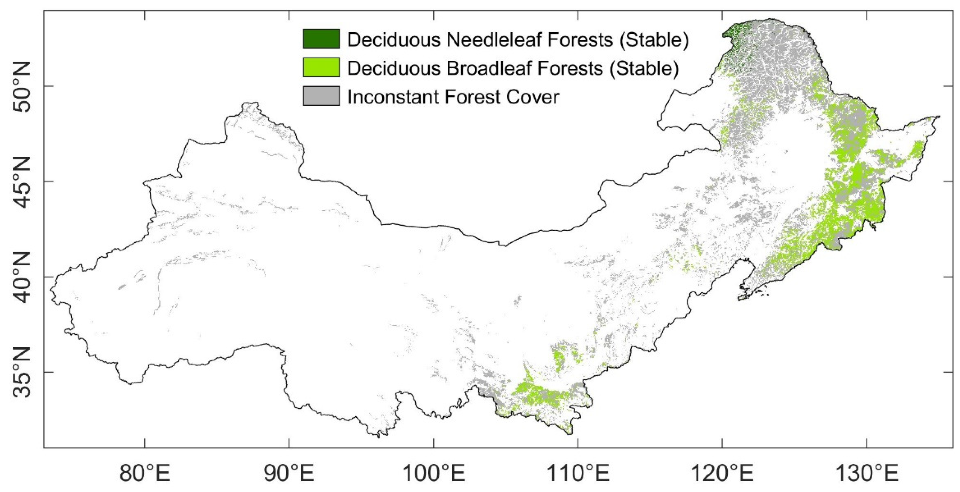
Our research objects were selected from the whole northern China. The climate here transitions from a temperate continental climate to a temperate monsoon climate. Despite the climate heterogeneity of northern China, forests distribute broadly in this area, helping maintain the sustainability of the ecosystem (Figure 1, the gray-colored background). Forest cover in northern China has been significantly altered in recent decades by afforestation, reforestation, and other human activities, which might have made the response of the forests to drought even more complicated. To disentangle the response characteristics of the typical forests in this region, we focused on forests where the landcover remained stable during our study period (2001–2015).
2.2. Data
2.2.1. Model Tree Ensemble GPP
Gross primary productivity (GPP) reflects the efficient of ecosystem photosynthesis, which quantify aspects of vegetation growth. Unfortunately, on the ground, there are only sparsely in situ flux measurements available for the GPP partitioning. Instead, we used a machine-learning method—model tree ensemble (MTE) [18]—to generate regional GPP from in situ flux measurements [20]. This method has been validated and used for regional to global carbon uptake analysis [16,21]. This GPP (hereafter MTE-GPP) was simulated at a spatial resolution of 0.1 degree and monthly temporal resolution, from 1981 to 2015. We resampled the MTE-GPP into 500 m before analyzing. The variables utilized in our simulation were listed in Table A1. Details of the data-driven product is available in Yao et al.’s work published in 2018 [20].
2.2.2. Satellite-Derived Vegetation Growth Data
Remote sensing data could reflect long time series and large-scale spatial information of vegetation. To compare with the response generated from MTE-GPP, the satellite-derived MODIS 500 m 16-day GPP product (MOD17A2H collection 6) was used, hereafter referred to as ‘GPP’ directly. Another type of satellite-derived vegetation index (enhanced vegetation index, EVI) has been widely used in previous researches about the responses of forests to droughts. The EVI describes the growth condition of canopies, and has been suggested as having improved sensitivity over high biomass regions, e.g., forests [22], compared to the other popular vegetation indices such as normalized difference vegetation index (NDVI). The responses of EVI to climate factor might be different from GPP, while only a few studies compared their performances on the responses of forests to drought [10,11]. To explore the differences between GPP and EVI, the MODIS 500 m 16-day vegetation index product (MOD13A1 Version 6) was chosen as EVI data source in our study, hereafter referred to as ‘EVI’ directly. It contains the global EVI values since 2001 to present. Both of the two datasets in our study area were mosaiced and extracted via Google Earth Engine (GEE). After that, we regenerated monthly EVI and GPP from these 16-day data, following an official procedure from MODIS team which considered days as weights [23]. The regeneration was performed in MATLAB.
2.2.3. Drought Index
The standardized precipitation evapotranspiration index (SPEI) was used for drought detecting in this study. The SPEI is a state-of-the-art meteorological drought index. It considered not only temperature and/or precipitation as the traditional drought index (e.g., PDSI and SPI), but also considered evapotranspiration (ET), which described the average water balance of the terrestrial ecosystem [24]. In this study, we downloaded the 12-month windowed SPEI (SPEI-12) dataset from the Global SPEI Database (https://spei.csic.es/database.html, 18 January 2021),since the annual water balance has been proved to be strongly correlated with forest growth [25]. The spatial resolution of this dataset is 0.5 degree. To make the pixels location fit to the MODIS EVI and GPP for spatial statistical analyses, we resampled the SPEI pixel into 500 m following the nearest neighbor rule.
2.2.4. Vegetation Category
The MODIS landcover data (MCD12Q1, version 006) and the vegetation map of China (1:1,000,000) were used for extracting and categorizing in our study. The vegetation map of China from the Institute of Botany of the Chinese Academy of Sciences [26] is derived from multi-source data, including forest inventory data, field samples, and remote sensing data [27]. Hence, this map reflects the vegetation in China more precisely than present remote sensing-based landcover data. This map is also used for MTE-GPP simulation among different vegetation ecosystems (see Table A1). Unfortunately, this map is neither dynamic nor near-real-time. Given the huge landcover changes during the last two decades in the northern China, we compared the vegetation map of China with the 500 m MCD12Q1 from 2001 to 2015, then selected those pixels which did not change in MCD12Q1 during 2001 to 2015, as well as were classified as the same forest type in both the vegetation map of China and MCD12Q1 (hereafter ‘stable pixels’). The vegetation map was transformed from vector to raster format with a 500 m spatial resolution. As a result, most of the stable pixels were deciduous broadleaf forest (DBF, 859,587 pixels in total) and deciduous needleleaf forest (DNF, 57,792 pixels in total). The spatial distribution of forest pixels for this study is shown in Figure 1.
2.3. Methods
2.3.1. Defining Levels of Water-Balance Condition and Consecutive Droughts
The water balance dynamics of different regions are spatially heterogeneous. In the meantime, the vegetation has generally adapted to certain local hydrothermal conditions. Therefore, we employed the commonly used meteorological definition, which was based on percentiles of water index, to categorize the water balance condition of each grid individually. Here, the levels of water-balance condition are defined by the thresholds of SPEI percentile in Table 1.
To count the percentile of historical SPEI of each pixel, we firstly sorted the mean SPEI12 of growing season (April to October) from 1902 to 2015 for each stable forest pixel. We did not include year 1901 because the 12-month window of SPEI12 made the valid SPEI12 values were available since December 1901. Then we sorted the 114 years’ SPEI12 of each pixel. We used the 11th lowest (which was approximately the 10th percentile of 114 values) SPEI12 values as the threshold for extreme drought, which corresponded to happening once per decade. In the meantime, the values between rank 12 to rank 28 (about the 25th percentile, suggested the climate events happen once per four years) corresponded to moderate drought, as well as the values between rank 29 (25th percentile) to rank 85 (75th percentile) suggested normal years. This classification was also used for detecting normal years for the ecosystem resistance and resilience calculation in this study.
The acclimation of vegetation to droughts might be differing as the frequency of perturbance changing [8,28,29]. Therefore, whether consecutive droughts happened before and after our most concerned year was also considered and discussed. Specifically, we explored whether the ecosystem stability of forests were different between droughts that were preceded either by normal or drought year. We also tested the recovery of forests by whether a subsequent drought happened after the drought year.
2.3.2. Ecosystem Resistance and Resilience
The ecosystem resistance stands for the ability of an ecosystem to maintain its status under disturbance, and the ecosystem resilience describes the capacity to recover from the disturbance [28]. Both of them are part of the ecosystem stability. To quantitate the resistance and resilience to drought in our study area, we utilized the two equations following Isbell et al.’s research [28]:
and
where Yn is the forest growth during normal years among 2001–2015, Ye is the forest growth during the event year, and Ye+i is the forest growth i years after the event year, i = 1, 2, and 4. We decided to use the changing i because legacy effect widely exists, and was suggested among one to four years for forests [29,30]. As a result, the water balance of the forests in the succeeding four years should also be considered. Hereafter, resistance would be mentioned as ‘Rt’, and resilience is ‘Rs’. Both of the Rt and Rs values were unitless, which made it convenient to compare the stability across varies biomes.
2.3.3. Standardization
A routine standardization (mean/standard deviation, μ/σ) method was used to preprocess the time series of monthly EVI, GPP, and MTE-GPP. The standardized results were then comparable for our research.
2.3.4. Pearson Correlation Analysis
The Pearson correlation analysis was employed to analyze if there is a trade-off between the ecosystem resistance and resilience, for each forest pixel. The student-t test was used to test the significance.
2.3.5. Analysis of Variance (ANOVA)
To detect if there is significant difference between DNF and DBF, one-way analysis of variance (one-way ANOVA) was conducted by using the MATLAB function ‘anova1’. The F-test result could describe the significance.
3. Results
3.1. Spatio-Temporal Characteristics of Droughts
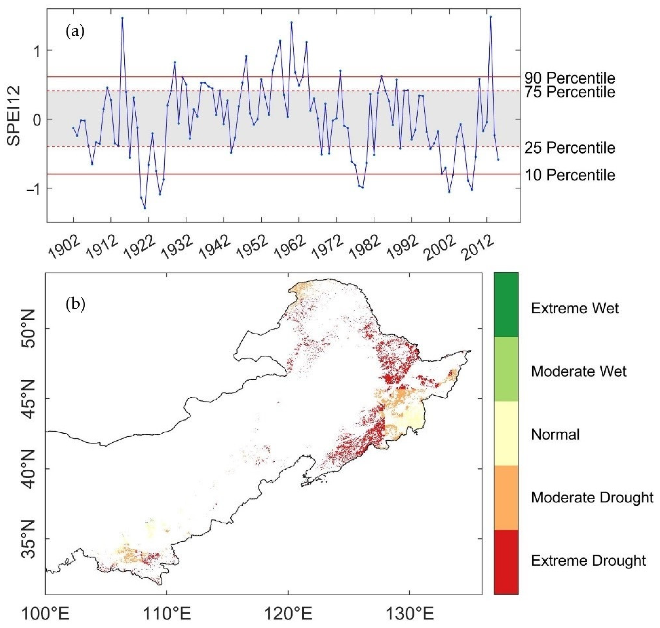
The time series of mean growing season SPEI 12 (Figure 2a) illustrated the overall drought condition from 1902 to 2015 for the stable forests. During the 114 years, forests in northern China experienced ten extreme drought events, which happened approximately once per decade. There were four of these extensive drought events occurred after year 2001, which were in 2002, 2003, 2007, and 2008. Despite the drought events in 2003 and 2003, forests were generally under normal water condition during 2004 to 2006. However, after the extreme and pervasive drought in 2007 and 2008, our study objects experienced dramatic fluctuations from moderate drought (2009) to moderate wet (2010), which might cause an even more complicated situation for comparing the ecosystem stability. Thus, we decided to focus on exploring the resistance and one-to-four-year resilience of forests to drought in 2002. The involved time period is 2001–2016.
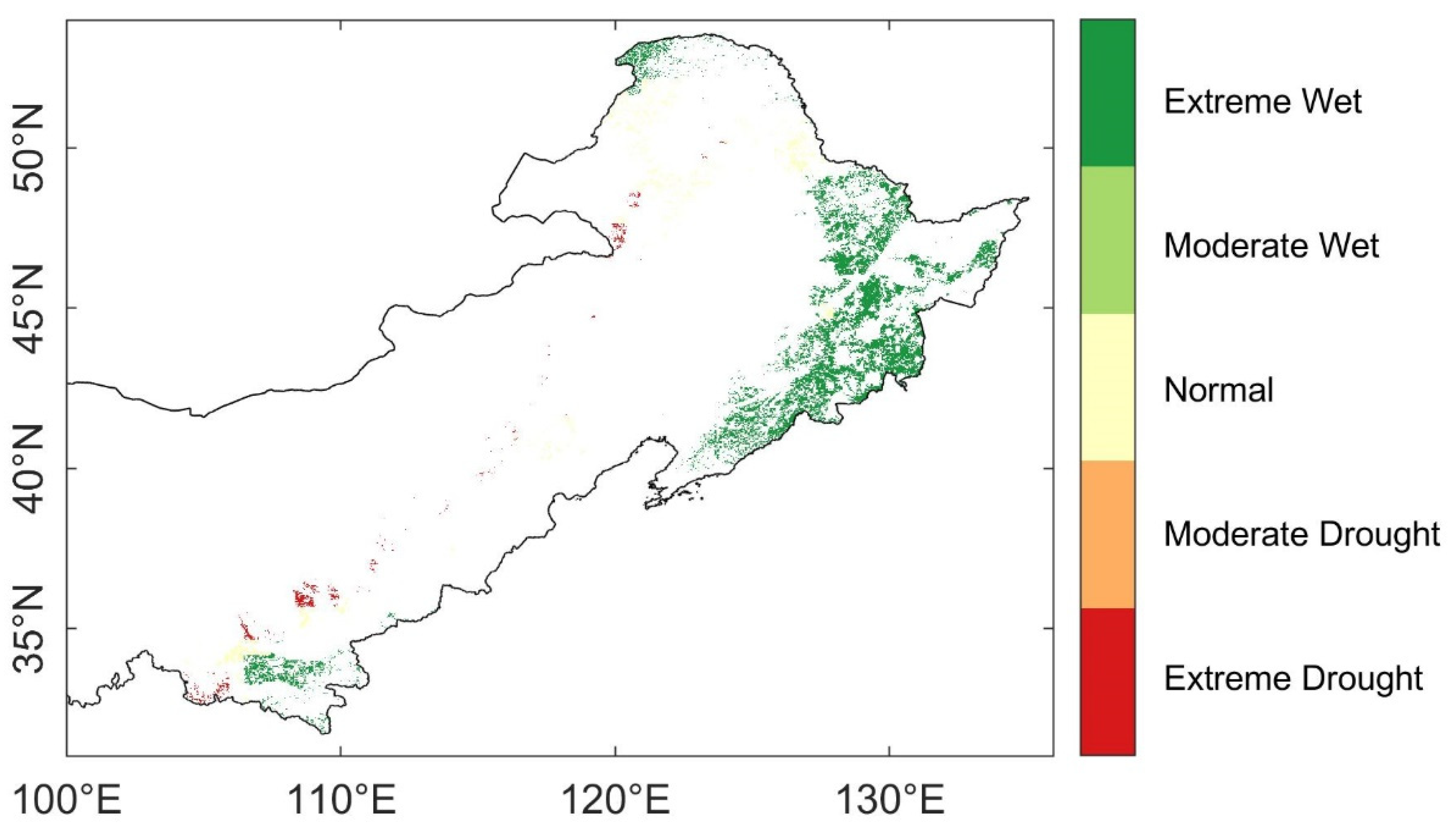
To classify the drought condition spatially, we retrieved the minimum SPEI12 during growing season in 2002 for each forest pixel. Unsurprisingly, most of the forests in northern China experienced drought under different levels in 2002 (Figure 2b). There were 97.37% of the forest pixels had a SPEI12 value lower than zero, in which 53.00% were under severe droughts (−2 < SPEI12 ≤ −1.5), and 23.65% experienced extreme droughts (SPEI12 ≤ −2). The severe and extreme drought regions were clustered in the northeast and east of northern China, which were covered with dense forests. Only 18.62% of the forest pixels were under moderate drought condition (−1.5 < SPEI12 ≤ −1). The result suggested that large areas of the forests in northern China experienced severe-to-extreme droughts in 2002.
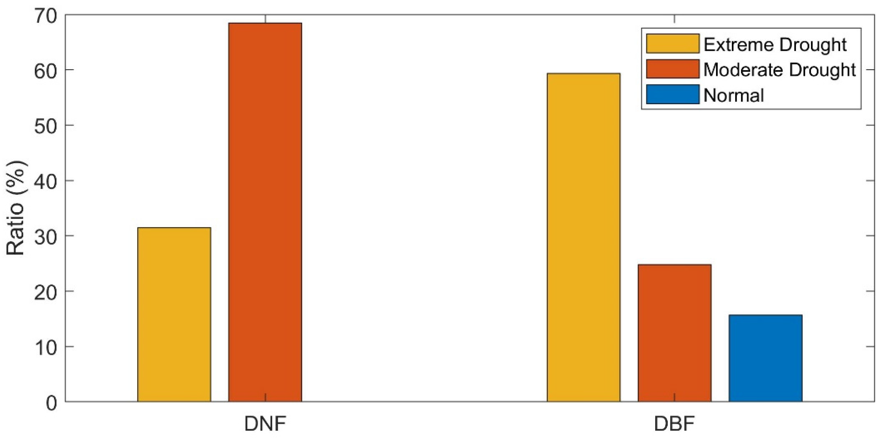
To compare the areas of the DNF and DBF under drought, we counted the ratio of DNF and DBF pixels under vary water condition separately. The majority of the DNFs experienced drought events, in which 31.45% encountered extreme drought, and 68.42% were under moderate drought in growing season in 2002. Only 0.13% of the DNFs were under normal to wet conditions. To the DBF pixels, 59.33% experienced extreme drought, 24.81% were under moderate drought, and 15.69% were under normal to wet conditions, respectively (Figure 3). Since drought events occurred extensively among our study objects, pixels under drought events in 2002 were selected for analyzing.
3.2. Interannual Variation of Forest Growth
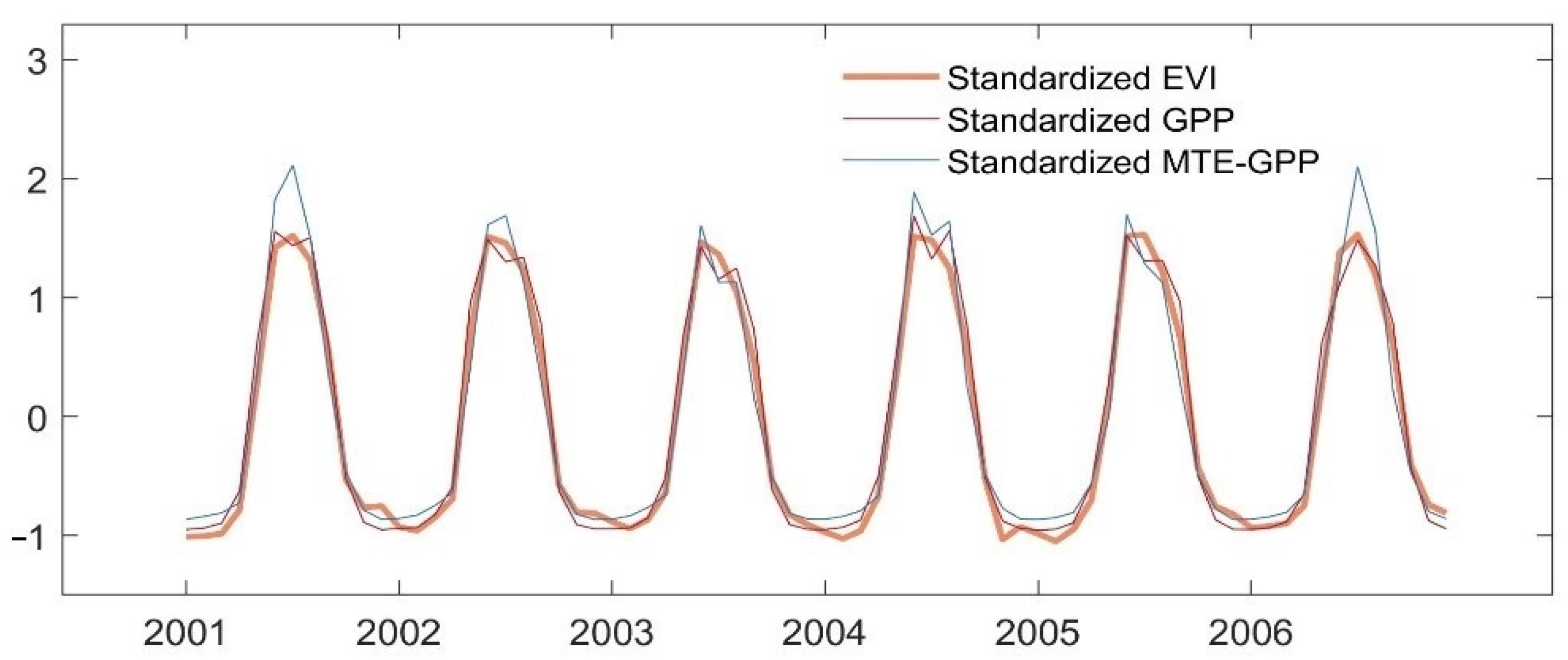
The time series of standardized monthly mean EVI, GPP, and MTE-GPP during 2001–206 showed similar interannual variations with slight differences (Figure 4). Interestingly, although the peak value of MTE-GPP was larger than GPP and EVI in 2001, their peak values were converging gradually after drought year in 2002. During 2003 to 2005, the variation of MTE-GPP and GPP were quite similar, until in the MTE-GPP showed a sudden increasing amplitude in 2006, which was four years after the drought year.
The similarity and differences among variations of the EVI, GPP, and MTE-GPP would lead to diverse ecosystem stability results, which might be reflected in spatial distribution or the differences between DNFs and DBFs.
3.3. Spatial Distribution of Ecosystem Stability of the Forests to Drought in 2002
We first explored the spatial distribution of the ecosystem stability of the forests in our study area. Hence, we calculated the resistance during 2002, and the resilience 1-, 2-, and 4-years after 2002, for each stable forest pixel.
3.3.1. The Resistance during Drought in 2002
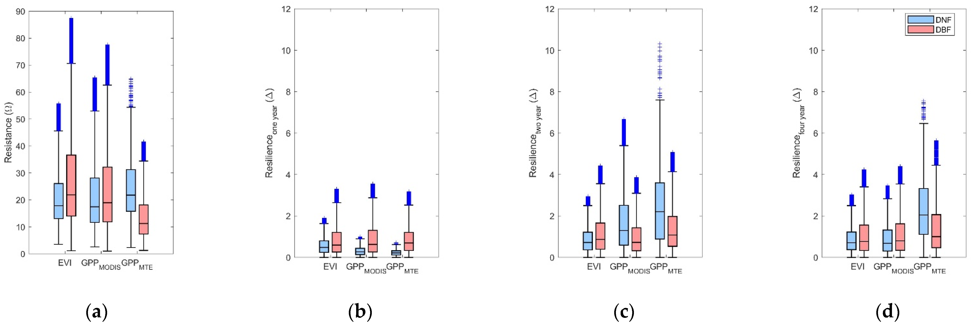
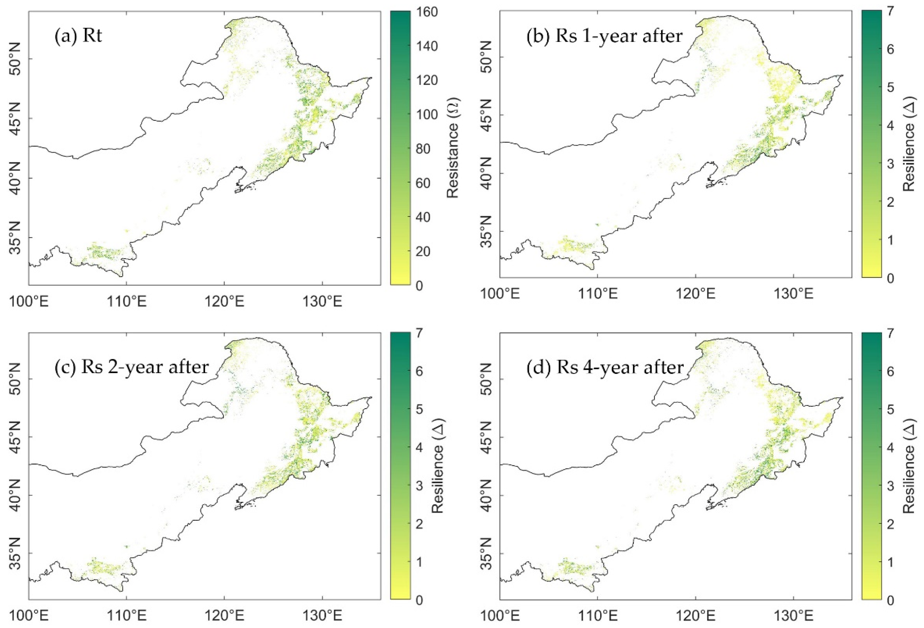
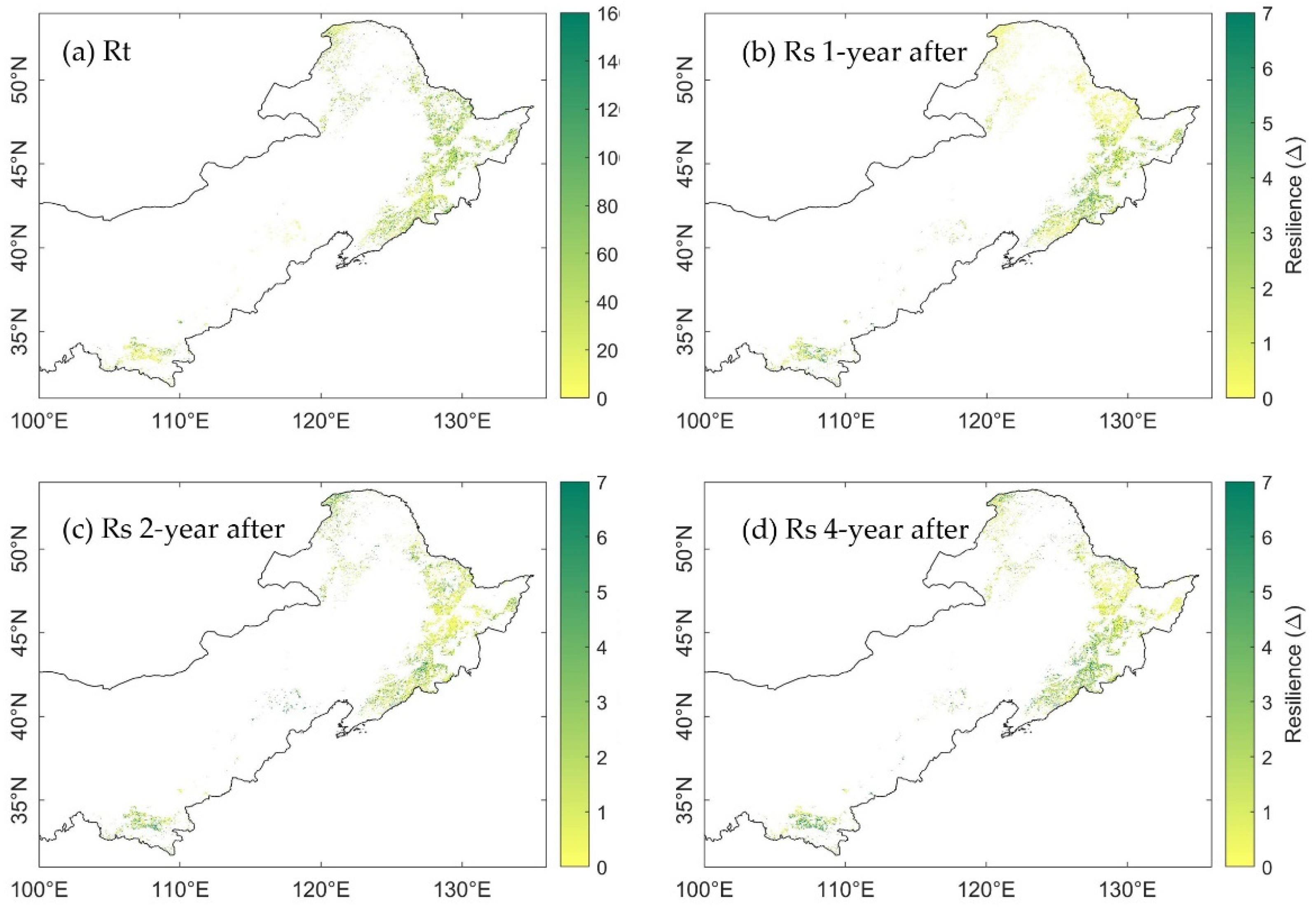
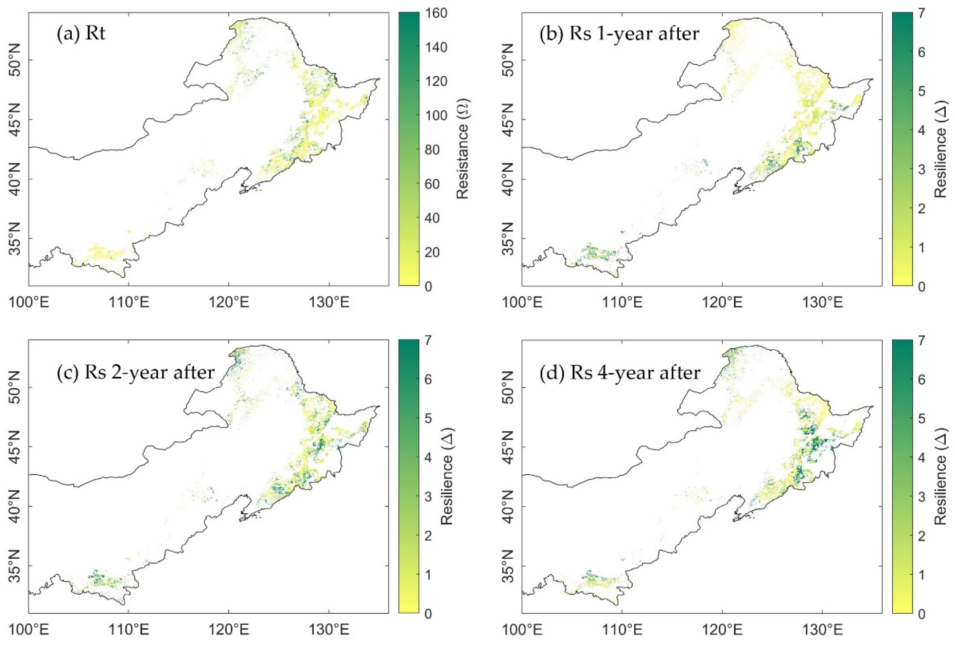
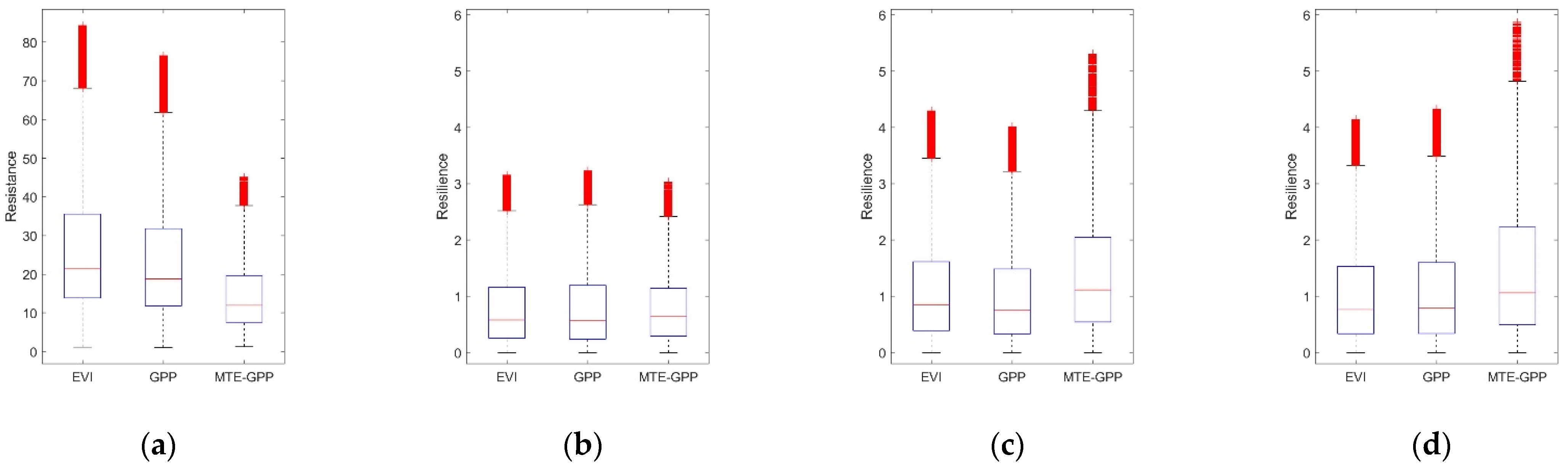
Generally, the range of RtEVI and RtGPP was similar, which was [1.16, 84.38] and [1.00, 76.58], respectively. The range of RtMTE-GPP was the smallest, between 1.25 and 45.17 (Figure 5a, outliers were excluded). This difference was due to the higher magnitude of MTE-GPP in 2001, which resulted in a relatively sharp decrease in the drought year 2002. The spatial distribution of resistance generated from EVI (RtEVI) and GPP (RtGPP) showed similar pattern (Figure 6a vs. Figure 7a), albeit the RtEVI were generally higher than the RtGPP. More than that, the spatial distribution of RtMTE-GPP was distinctly different from that of RtEVI and RtGPP (Figure 8a). In the north area, the high values of RtMTE-GPP was not only higher, but also more spatial-clustered than the other two spatial distributions. Meanwhile, many pixels illustrated opposite results between RtMTE-GPP and RtEVI with RtGPP. The pixels with RtEVI and RtGPP higher than 100 often had a RtEVI value lower than 20 in both the east and the south of the study area. The results implicated different response regimes of MODIS-EVI, MODIS-GPP, and MTE-GPP to drought.
3.3.2. The Resilience at 1-, 2-, and 4-Years after the 2002 Drought
The resilience 1-year after 2002 drought calculated from EVI (RsEVI-1), GPP (RsGPP-1), and MTE-GPP (RsMTE-GPP-1) showed seemingly trade-off spatial patterns to the resistance in 2002 (Figure 6b, Figure 7b and Figure 8b). However, the overall resilience 1-year after the drought were similar among EVI, GPP, and MTE-GPP (Figure 5b). The median Rs from EVI, GPP, and MTE-GPP were 0.58, 0.57, and 0.65, respectively, which implied similar recovery levels of canopy and gross photosynthesis.
The spatial distribution of resilience 2-years after the 2002 drought was different from the 1-year after resilience. Rs calculated from EVI, GPP, and MTE-GPP all illustrated higher recovery, especially in the northeast of the study area (Figure 6c, Figure 7c and Figure 8c). These changes supported the perspective that forests generally need more than one year to recover from annual droughts.
When it came to the fourth year (2006) after the 2002 drought, the overall mean growing season SPEI12 was exactly at the 25th percentile, which was the threshold of normal year and moderate drought. The changes of the resilience were unevenly distributed as RsEVI-4, RsGPP-4, and RsMTE-GPP-4 shown (Figure 6d, Figure 7d and Figure 8d). Some areas showed continuously increasing resilience, while some others’ resilience decreased. The inconsistency might be due to the spatial heterogeneity of hydrothermal conditions. These results called for further comparison considering the water balance condition pixel-by-pixel.
3.4. Stability of DBF and DNF to Drought in 2002
3.4.1. Comparison of the Resistance during 2002 between DBF and DNF
The resistance of DNF pixels (blue box) and DBF pixels (pink box) during 2002 is shown in Figure 5a. The median resistance values of DNF calculated from EVI, GPP, and MTE-GPP were 17.85, 17.45, and 21.78, respectively. The median resistance values of DBF were 21.86, 18.95, and 11.26, respectively. Resistance of DNF based on MTE-GPP was higher than that based on EVI and GPP. Meanwhile, resistance of DBF was significantly lower from MTE-GPP. Although the values among EVI, GPP, and MTE-GPP were different, the significant differences are prevalent between NF and BF in the three datasets (Table A2).
3.4.2. Comparison of the Resilience 1-, 2-, and 4-Year after Drought between DNF and DBF
The resilience of stable DNF and DBF pixels 1-, 2-, and 4-years after the drought in 2002 was shown in Figure 8b–d. The values of Rs 2-years after the 2002 drought were significantly higher than the ones 1-year after the 2002 drought (Figure 5b,c). Interestingly, the Rs of the DBF 1-year after the 2002 drought was higher than that of the DNF, while the Rs 2-year after 2002 drought illustrated a reverse relationship. The Rs in 2006 (Figure 5d), which was four years after the 2002 droughts illustrated similar results as the Rs in 2004 (Figure 5c), although the Rs in 2006 displayed more convergence. As most stable pixels were under moderate extreme wet conditions, both among the DNF and DBF (Figure A2), the resilience in different years indicated that both the DNF and DBF would fully recover in four years. Furthermore, similar to the resistance, significant differences are prevalent between the resilience of DNF and DBF in the three datasets (Table A2).
4. Discussion
4.1. Comparison among Interannual Variation of EVI, GPP, and MTE-GPP
MTE-GPP and GPP generally showed similar variations along the 1–3 years after the drought year. However, the lower GPP value before and during 2002 drought led to higher resistance from the MODIS-GPP. This bias may be due to the simplification of the LUE modeling approach employed by the MODIS-GPP, which could not precisely depict the vegetation photosynthesis before, during, and after disturbances. On the other hand, the subtle differences between variation of EVI and GPP might come from the different vegetation activities that EVI and GPP reflected. EVI is an index indirectly reflected the physical characteristics of the plant canopy such as phytochrome and water content [31], while GPP is a physiological indicator that is directly influenced by a range of ecological factors [16,32]. Therefore, the response of EVI to drought can be considered as the response of physical condition of leaves to drought. This information indicated that if one meteorological drought event did not damage the canopy, the EVI might not show response to this drought. Prior studies have shown that EVI only responded to drought when the canopy was damaged [33]. Hence, MTE-GPP might be more suitable for assessing the response of forest to seasonal to annual droughts than both MODIS-GPP and MODIS-EVI.
4.2. Differences between Ecosystem Stability of DNF and DBF
The spatial trade-off between resistance and resilience of all DNF and DBF in northern China was shown in this study (Figure 6, Figure 7 and Figure 8), which corresponded to previous studies [28]. However, the differences of ecosystem stability between DNF and DBF showed complicated characteristics. None of the ecosystem stability of DNF and DBF were similar, as the one-way ANOVA results shown in Table A2. This result implies that the balance between resistance and resilience might be biome-or-species-specific. Research on certain species has drawn similar conclusions—the stability of different biomes are heterogeneous [7,34]. Besides, the resilience of the DBF 1–4 year after the drought was relatively stable, which suggested faster recovery of the DBF than the DNF. Meanwhile, the DNF recovered more than the DBF in the second year after the drought. The result indicated that temporal trade-off of the DBF and DNF might not only exist along timescale for decades, but also along shorter timescale such as interannual. Moreover, higher Rs 2-years after the drought for the DNF from GPP and MTE-GPP indicated that the GPP is more sensitive to annual drought than EVI.
4.3. Comparison of Ecosystem Stability Considering Consecutive Drought
Research has mentioned the importance of drought frequency in studying stability of forest to drought [8,29]. For this reason, the influence of consecutive droughts was considered and discussed in this section.
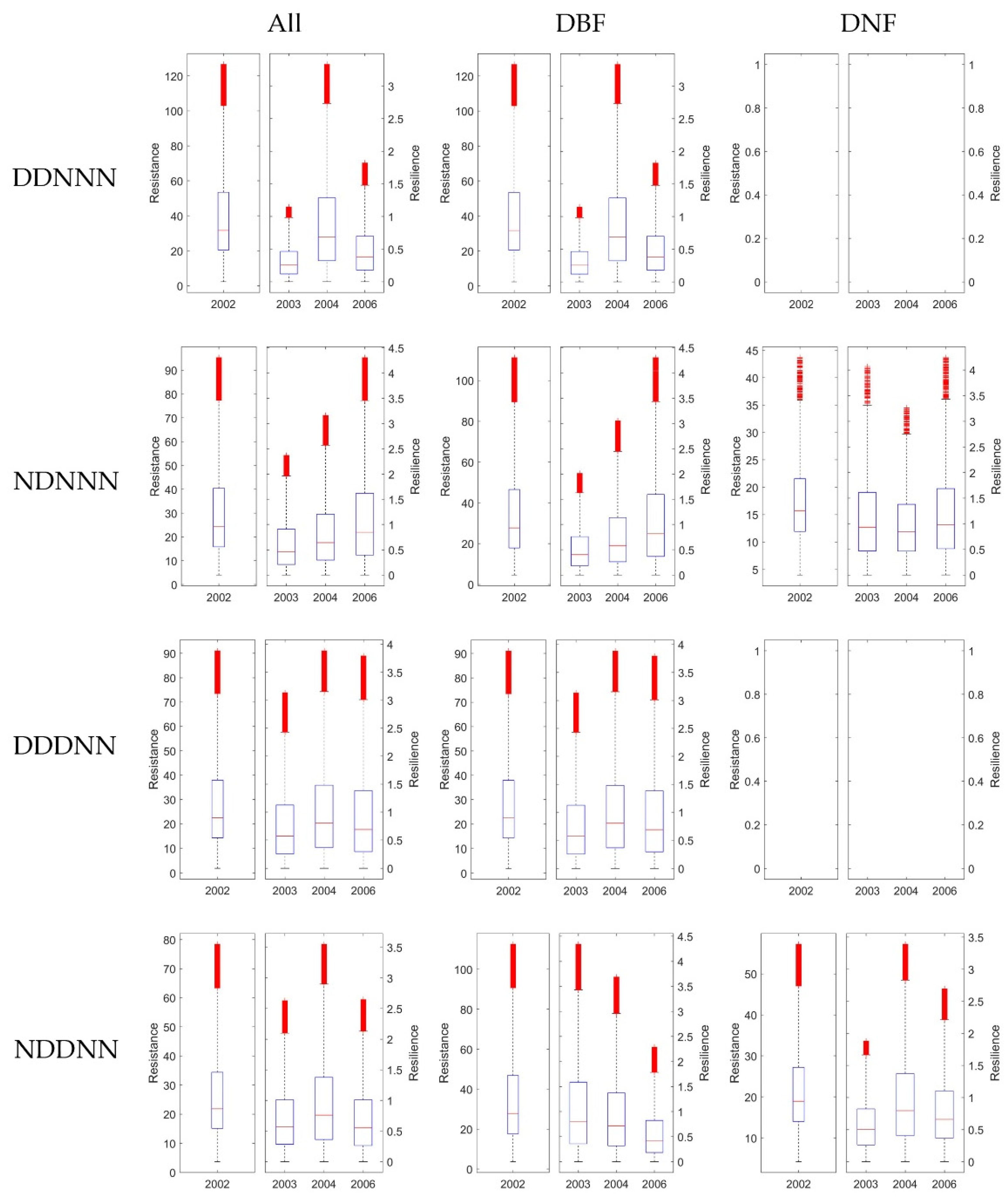
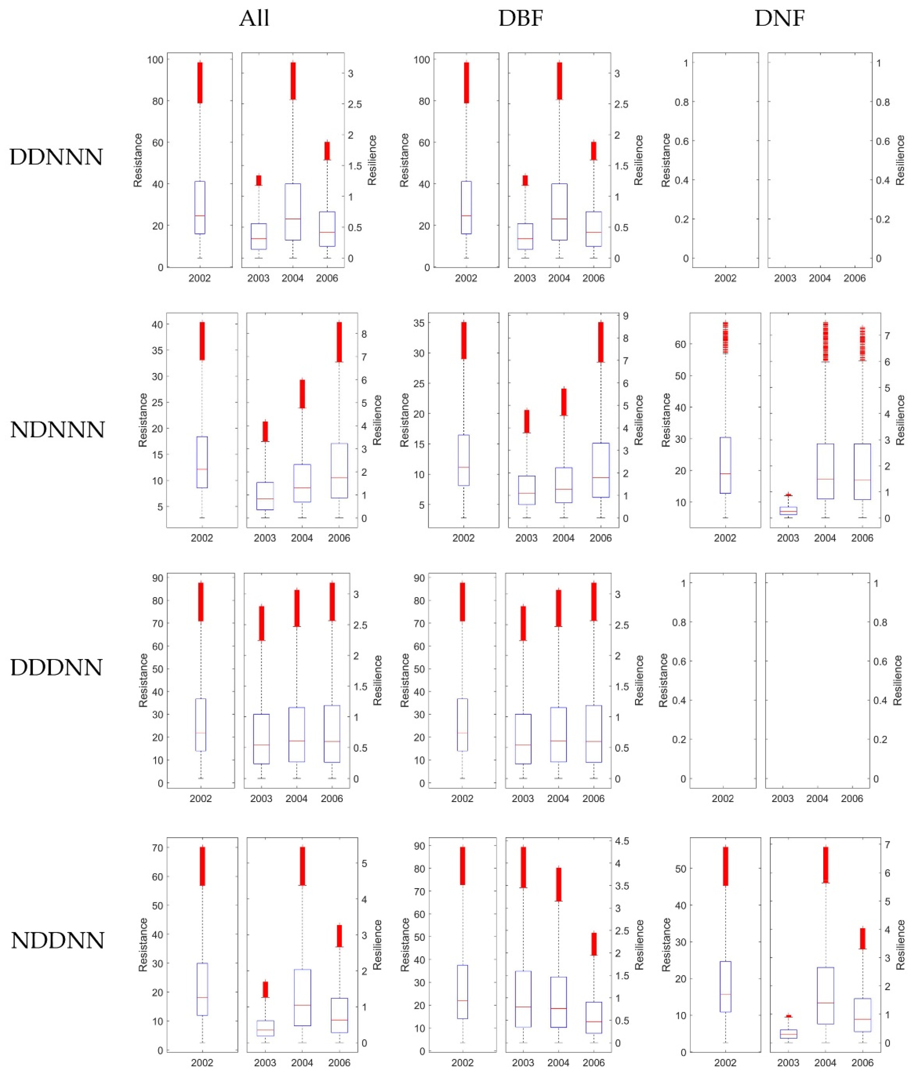
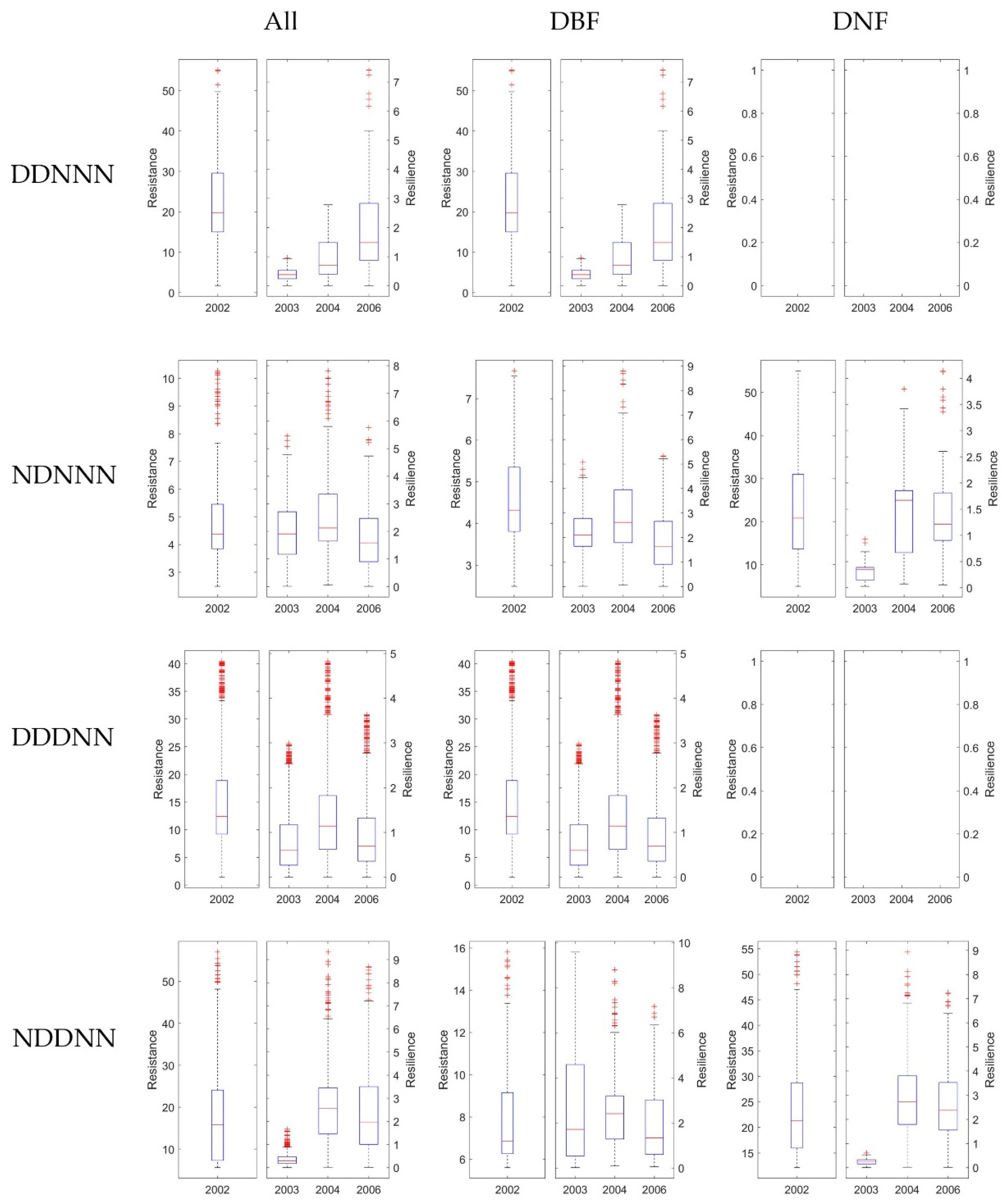
It is difficult to fully explore the effects of varies consecutive drought combinations for multi-years. To simplify the scenarios, we only considered four typical water balance conditions in this study. First, we divided the pixels of stable forests by whether the year 2001 was a normal year for the pixel, which might influence the result of the resistance. Second, we classified the pixels by whether the year after the drought was a normal year. For the rest of the years, we only picked pixels under normal water balance conditions. This selection criterion could simplify and better help to quantify the recovery of the forest after no more than three consecutive years of drought. As a result, four climate combinations were grouped. Figure 9, Figure 10 and Figure 11 showed the classified results generated from EVI, GPP, and MTE-GPP, respectively. All of the results showed that the forests that experienced drought in 2001—which were all DBF pixels—had a higher resistance in 2002, or the DBF could quickly acclimate to drought, and would decrease less under two-year consecutive droughts than under a single annual drought. The results from MTE-GPP and the MODIS products were slightly different. Generally, the resilience in 2006 was lower than in 2004 without experiencing drought. The result suggested that the response mechanism of forests to water-balance might involve more driving factors than temperature and water. Additionally, for pixels in which 2003, 2004, and 2006 were normal years, the DBF illustrated increasing resilience for all the three years after drought. Hence, the DBF might have acclimated better to various hydrothermal conditions than the DNF, and could even enhance the growth when the climate condition is suitable.
5. Conclusions
Based on one machine-learning simulation result and two remote sensing-derived datasets of vegetation growth, we found that EVI and GPP showed the response of forests to drought diversely, because they reflected the ecosystem stability of forests from different perspectives. Although a spatial trade-off exists broadly in forests in northern China, this correlation is non-linear. Moreover, the ecosystem stability is community-, biome-, or species-specific. The resistance and resilience also illustrated temporal trade-offs at a yearly timescale, as well as that the DBF was better acclimatized to drought disturbances. These results can provide information for forest management to consult in the future for a higher-frequency extreme events context. The comparison among MODIS-EVI, MODIS-GPP, and MTE-GPP suggested that MTE-GPP could be used for evaluating the response of forests to drought. Last but not least, both the MTE and satellite-based approaches of simulating GPP can be further improved by considering the variables and processes in more details.
Author Contributions
Conceptualization, X.L.; Formal Analysis, G.Y.; Funding Acquisition, X.L.; Methodology, X.L., Y.Y. and G.Y.; Software, Y.Y.; Writing—Original Draft, X.L.; Writing—Review and Editing, X.L., F.P. and M.L. All authors have read and agreed to the published version of the manuscript.
Funding
This research was funded by the National Natural Science Foundation of China (NSFC), grant number 41901112, and the Natural Science Foundation of Hubei Province of China, grant number ZRMS2019002066.
Institutional Review Board Statement
Not applicable.
Informed Consent Statement
Not applicable.
Data Availability Statement
The data presented in this study are available on request from the corresponding websites or authors.
Conflicts of Interest
The authors declare no conflict of interest.
Appendix A

Table A1.
Variables for MTE-GPP simulation (similar to Yao et al., 2018 [20]).
Table A1.
Variables for MTE-GPP simulation (similar to Yao et al., 2018 [20]).
| Variable | Type | Type of Variability |
|---|---|---|
| Mean annual temperature | Split | Static |
| Mean annual temperature maximum | Split | Static |
| Mean annual precipitation sum | Split | Static |
| Mean annual radiation | Split | Static |
| Mean annual FPAR | Split | Static |
| Mean monthly temperature | Split | Monthly but static over years |
| Mean monthly temperature maximum | Split | Monthly but static over years |
| Mean monthly precipitation sum | Split | Monthly but static over years |
| Mean monthly radiation | Split | Monthly but static over years |
| Mean monthly FPAR | Split | Monthly but static over years |
| Monthly temperature | Split & Regression | Monthly |
| Monthly temperature maximum | Split & Regression | Monthly |
| Monthly precipitation | Split & Regression | Monthly |
| Monthly precipitation a month before | Split & Regression | Monthly |
| Monthly radiation | Split & Regression | Monthly |
| Monthly FPAR | Split & Regression | Monthly |
| Vegetation type | Split | Static |
Table A2.
One-way ANOVA between DNF and DBF.
| ‘SS’ | ‘df’ | ‘MS’ | ‘F’ | ‘Prob > F’ | |
|---|---|---|---|---|---|
| EVI-Rt | 2.14 × 10+6 | 1 | 2.14 × 10+6 | 6.53 × 10+3 | 0 |
| EVI-Rs 1 | 3.68 × 10+3 | 1 | 3.68 × 10+3 | 6.58 × 10+3 | 0 |
| EVI-Rs 2 | 4.55 × 10+3 | 1 | 4.55 × 10+3 | 4.62 × 10+3 | 0 |
| EVI-Rs 3 | 2.12 × 10+3 | 1 | 2.12 × 10+4 | 1.74 × 10+4 | 0 |
| EVI-Rs 4 | 2.06 × 10+3 | 1 | 2.06 × 1003 | 2.21 × 10+3 | 0 |
| GPP-Rt | 2.93 × 10+5 | 1 | 2.93 × 10+5 | 1.09 × 10+3 | 8.365 × 10−238 |
| GPP-Rs1 | 1.09 × 10+4 | 1 | 1.09 × 10+4 | 2.80 × 10+4 | 0 |
| GPP-Rs 2 | 2.65 × 10+4 | 1 | 2.65 × 10+4 | 2.98 × 10+4 | 0 |
| GPP-Rs 3 | 1.80 × 10+3 | 1 | 1.80 × 10+3 | 2.02 × 10+3 | 0 |
| GPP-Rs 4 | 1.90 × 10+3 | 1 | 1.90 × 10+3 | 1.88 × 10+3 | 0 |
| MTEGPP-Rt | 5.38 × 10+6 | 1 | 5.38 × 10+6 | 6.23 × 10+4 | 0 |
| MTEGPP-Rs1 | 2.03 × 10+4 | 1 | 2.03 × 10+4 | 4.21 × 10+4 | 0 |
| MTEGPP-Rs 2 | 6.79 × 10+4 | 1 | 6.79 × 10+4 | 4.45 × 10+4 | 0 |
| MTEGPP-Rs 3 | 2.95 × 10+5 | 1 | 2.95 × 10+5 | 2.81 × 10+5 | 0 |
| MTEGPP-Rs 4 | 3.84 × 10+4 | 1 | 3.84 × 10+4 | 2.19 × 10+4 | 0 |
Figure A1.
The range of (a) resistance during 2002; (b) resilience one year after 2002; (c) resilience two-year after 2002; and (d) resilience four-year after 2002.
Figure A1.
The range of (a) resistance during 2002; (b) resilience one year after 2002; (c) resilience two-year after 2002; and (d) resilience four-year after 2002.

Figure A2.
The water balance classification in 2006.

References
- Ding, Y.; Xu, J.; Wang, X.; Peng, X.; Cai, H. Spatial and temporal effects of drought on Chinese vegetation under different coverage levels. Sci. Total Environ. 2020, 716, 137166. [Google Scholar] [CrossRef]
- Liang, E.; Shao, X.; Kong, Z.; Lin, J. The extreme drought in the 1920s and its effect on tree growth deduced from tree ring analysis: A case study in North China. Ann. For. Sci. 2003, 60, 145–152. [Google Scholar] [CrossRef] [Green Version]
- Ji, S.; Ren, S.; Li, Y.; Dong, J.; Wang, L.; Quan, Q.; Liu, J. Diverse responses of spring phenology to preseason drought and warming under different biomes in the North China Plain. Sci. Total Environ. 2021, 766, 144437. [Google Scholar] [CrossRef] [PubMed]
- Williams, A.P.; Allen, C.D.; Macalady, A.K.; Griffin, D.; Woodhouse, C.A.; Meko, D.M.; Swetnam, T.W.; Rauscher, S.A.; Seager, R.; Grissino-Mayer, H.D.; et al. Temperature as a potent driver of regional forest drought stress and tree mortality. Nat. Clim. Chang. 2013, 3, 292–297. [Google Scholar] [CrossRef]
- Hartmann, H.; Moura, C.F.; Anderegg, W.R.L.; Ruehr, N.K.; Salmon, Y.; Allen, C.D.; Arndt, S.K.; Breshears, D.D.; Davi, H.; Galbraith, D.; et al. Research frontiers for improving our understanding of drought-induced tree and forest mortality. New Phytol. 2018, 218, 15–28. [Google Scholar] [CrossRef] [PubMed] [Green Version]
- Reich, P.B.; Sendall, K.M.; Stefanski, A.; Wei, X.; Rich, R.L.; Montgomery, R.A. Boreal and temperate trees show strong acclimation of respiration to warming. Nature 2016, 531, 633–636. [Google Scholar] [CrossRef]
- Gazol, A.; Camarero, J.J.; Guti, E.; Novak, K.; T, V.R.P.A.; Ribas, M.; Garc, I.; Alvaro, S.; Galv, J.D. Forest resilience to drought varies across biomes. Glob. Chang. Biol. 2018, 2143–2158. [Google Scholar] [CrossRef]
- Anderegg, W.R.L.; Trugman, A.T.; Badgley, G.; Konings, A.G.; Shaw, J. Divergent forest sensitivity to repeated extreme droughts. Nat. Clim. Chang. 2020, 10, 1091–1095. [Google Scholar] [CrossRef]
- Li, X.; Piao, S.; Wang, K.; Wang, X.; Wang, T.; Ciais, P.; Chen, A.; Lian, X.; Peng, S.; Peñuelas, J. Temporal trade-off between gymnosperm resistance and resilience increases forest sensitivity to extreme drought. Nat. Ecol. Evol. 2020, 4, 1075–1083. [Google Scholar] [CrossRef]
- Kannenberg, S.A.; Novick, K.A.; Alexander, M.R.; Maxwell, J.T.; Moore, D.J.P.; Phillips, R.P.; Anderegg, W.R.L. Linking drought legacy effects across scales: From leaves to tree rings to ecosystems. Glob. Chang. Biol. 2019, 25, 2978–2992. [Google Scholar] [CrossRef]
- Huang, K.; Xia, J. High ecosystem stability of evergreen broadleaf forests under severe droughts. Glob. Chang. Biol. 2019, 25, 3494–3503. [Google Scholar] [CrossRef]
- Gong, Z.; Zhao, S.; Gu, J. Correlation analysis between vegetation coverage and climate drought conditions in North China during 2001–2013. J. Geogr. Sci. 2017, 27, 143–160. [Google Scholar] [CrossRef]
- Weiss, S.M.; Kulikowski, C.A. Computer Systems That Learn: Classification and Prediction Methods from Statistics, Neural Nets, Machine Learning, and Expert Systems; M. Kaufmann Publishers: San Mateo, CA, USA, 1991; ISBN 1558600655. [Google Scholar]
- Bastos, A.; Ciais, P.; Friedlingstein, P.; Sitch, S.; Pongratz, J.; Fan, L.; Wigneron, J.P.; Weber, U.; Reichstein, M.; Fu, Z.; et al. Direct and seasonal legacy effects of the 2018 heat wave and drought on European ecosystem productivity. Sci. Adv. 2020, 6, 1–14. [Google Scholar] [CrossRef]
- Zan, M.; Zhou, Y.; Ju, W.; Zhang, Y.; Zhang, L.; Liu, Y. Performance of a two-leaf light use efficiency model for mapping gross primary productivity against remotely sensed sun-induced chlorophyll fluorescence data. Sci. Total Environ. 2018, 613–614, 977–989. [Google Scholar] [CrossRef] [PubMed]
- Beer, C.; Reichstein, M.; Tomelleri, E.; Ciais, P.; Jung, M.; Carvalhais, N.; Rödenbeck, C.; Arain, M.A.; Baldocchi, D.; Bonan, G.B.; et al. Terrestrial gross carbon dioxide uptake: Global distribution and covariation with climate. Science (80-.) 2010, 329, 834–838. [Google Scholar] [CrossRef] [PubMed] [Green Version]
- Ichii, K.; Ueyama, M.; Kondo, M.; Saigusa, N.; Kim, J.; Alberto, M.C.; Ardö, J.; Euskirchen, E.S.; Kang, M.; Hirano, T.; et al. New data-driven estimation of terrestrial CO2 fluxes in Asia using a standardized database of eddy covariance measurements, remote sensing data, and support vector regression. J. Geophys. Res. Biogeosci. 2017, 122, 767–795. [Google Scholar] [CrossRef]
- Jung, M.; Reichstein, M.; Bondeau, A. Towards global empirical upscaling of FLUXNET eddy covariance observations: Validation of a model tree ensemble approach using a biosphere model. Biogeosciences 2009, 6, 2001–2013. [Google Scholar] [CrossRef] [Green Version]
- Wu, X.; Hao, Z.; Hao, F.; Zhang, X. Variations of compound precipitation and temperature extremes in China during 1961–2014. Sci. Total Environ. 2019, 663, 731–737. [Google Scholar] [CrossRef] [PubMed]
- Yao, Y.; Wang, X.; Li, Y.; Wang, T.; Shen, M.; Du, M.; He, H.; Li, Y.; Luo, W.; Ma, M.; et al. Spatiotemporal pattern of gross primary productivity and its covariation with climate in China over the last thirty years. Glob. Chang. Biol. 2018, 24, 184–196. [Google Scholar] [CrossRef] [PubMed]
- Deng, Y.; Wang, X.; Wang, K.; Ciais, P.; Tang, S.; Jin, L.; Li, L.; Piao, S. Responses of vegetation greenness and carbon cycle to extreme droughts in China. Agric. For. Meteorol. 2021, 298–299, 108307. [Google Scholar] [CrossRef]
- Huete, A.R.; Didan, K.; Van Leeuwen, W. Modis Vegetation Index. Veg. Index Phenol. Lab 1999, 3, 129. [Google Scholar]
- Solano, R.; Didan, K.; Jacobson, A.; Huete, A. MODIS Vegetation Index User ’ s Guide (MOD13 Series). Univ. Arizona 2010, 2010, 38. [Google Scholar]
- Vicente-Serrano, S.M.; Beguería, S.; López-Moreno, J.I. A multiscalar drought index sensitive to global warming: The standardized precipitation evapotranspiration index. J. Clim. 2010, 23, 1696–1718. [Google Scholar] [CrossRef] [Green Version]
- Wang, S.; Fu, B.J.; He, C.S.; Sun, G.; Gao, G.Y. A comparative analysis of forest cover and catchment water yield relationships in northern China. For. Ecol. Manag. 2011, 262, 1189–1198. [Google Scholar] [CrossRef]
- Editorial Board of Vegetaion Map of China. Vegetation Map of the People’s Republic of China (1:1000000) (Digital Version), 1st ed.; Editorial Board of Vegetation Map of China, Ed.; Geology Press: Beijing, China, 2007; ISBN 9787503142888. [Google Scholar]
- Su, Y.; Guo, Q.; Hu, T.; Guan, H.; Jin, S.; An, S.; Chen, X.; Guo, K.; Hao, Z.; Hu, Y.; et al. An updated Vegetation Map of China (1:1000000). Sci. Bull. 2020, 65, 1125–1136. [Google Scholar] [CrossRef]
- Isbell, F.; Craven, D.; Connolly, J.; Loreau, M.; Schmid, B.; Beierkuhnlein, C.; Bezemer, T.M.; Bonin, C.; Bruelheide, H.; De Luca, E.; et al. Biodiversity increases the resistance of ecosystem productivity to climate extremes. Nature 2015, 526, 574–577. [Google Scholar] [CrossRef]
- Anderegg, W.R.L.; Schwalm, C.; Biondi, F.; Camarero, J.J.; Koch, G.; Litvak, M.; Ogle, K.; Shaw, J.D.; Shevliakova, E.; Williams, A.P.; et al. Pervasive drought legacies in forest ecosystems and their implications for carbon cycle models. Science (80-) 2015, 349, 528–532. [Google Scholar] [CrossRef] [Green Version]
- Schwalm, C.R.; Anderegg, W.R.L.; Michalak, A.M.; Fisher, J.B.; Biondi, F.; Koch, G.; Litvak, M.; Ogle, K.; Shaw, J.D.; Wolf, A.; et al. Global patterns of drought recovery. Nature 2017, 548, 202–205. [Google Scholar] [CrossRef] [PubMed]
- Huete, A.; Didan, K.; Miura, T.; Rodriguez, E.P.; Gao, X.; Ferreira, L.G. Overview of the radiometric and biophysical performance of the MODIS vegetation indices. Remote Sens. Environ. 2002, 83, 195–213. [Google Scholar] [CrossRef]
- Clark, D.A.; Brown, S.; Kicklighter, D.W.; Chambers, J.Q.; Thomlinson, J.R.; Ni, J. Measuring net primary production in forests: Concepts and field methods. Ecol. Appl. 2001, 11, 356–370. [Google Scholar] [CrossRef]
- Decuyper, M.; Chávez, R.O.; Čufar, K.; Estay, S.A.; Clevers, J.G.P.W.; Prislan, P.; Gričar, J.; Črepinšek, Z.; Merela, M.; de Luis, M.; et al. Spatio-temporal assessment of beech growth in relation to climate extremes in Slovenia—An integrated approach using remote sensing and tree-ring data. Agric. For. Meteorol. 2020, 287, 107925. [Google Scholar] [CrossRef]
- Pennington, R.T.; Lavin, M. The contrasting nature of woody plant species in different neotropical forest biomes reflects differences in ecological stability. New Phytol. 2016, 210, 25–37. [Google Scholar] [CrossRef] [PubMed] [Green Version]
Figure 1.
Spatial distribution of forests in the northern China. The emerald pixels were deciduous needleleaf forests which were stable during 2001–2015; the light green pixels were deciduous broadleaf forests which were stable during 2001–2015; the gray-colored pixels were forests which landcover might have changed during 2001–2015, or inconstant between the landcover datasets ‘China Vegetation Map’ and MODIS landcover product (MCD12Q1).

Figure 2.
Spatial and temporal characteristics of SPEI12: (a) The time series of mean growing season (April to October) SPEI 12 during 1902–2015 (blue line) and the overall percentiles of the stable pixels (solid red lines for 10th and 90th percentile, which stands for extreme drought and extreme wet event thresholds; dashed red lines for the 25th and 75th percentile, which stands for moderate drought and moderate wet even thresholds; and the gray-colored range marked the SPEI values of normal years); (b) the spatial distribution of water-balance condition in 2002 for the stable forest pixels, the climate events were classified with individual SPEI12 thresholds calculated from the 1902–2015 records of each pixels respectively.

Figure 3.
The ratio of forest areas under different water balance conditions in 2002. DNF stands for the stable deciduous needleleaf forest pixels, and DBF stands for the stable deciduous broadleaf forest pixels.
Figure 3.
The ratio of forest areas under different water balance conditions in 2002. DNF stands for the stable deciduous needleleaf forest pixels, and DBF stands for the stable deciduous broadleaf forest pixels.

Figure 4.
Interannual variations of standardized monthly EVI (orange line), GPP (red line), and MTE-GPP (blue line) during 2001–2006.
Figure 4.
Interannual variations of standardized monthly EVI (orange line), GPP (red line), and MTE-GPP (blue line) during 2001–2006.

Figure 5.
Boxplot of (a) resistance during 2002; (b) resilience one year after 2002 drought; (c) resilience two years after 2002 drought; and (d) resilience four years after 2002 drought. Outliers were removed. The blue box stands for values of stable DNF. The pink box stands for values of stable DBF.

Figure 6.
Spatial distribution of (a) resistance to drought in 2002; (b) resilience 1-year after 2002 drought; (c) resilience 2-years after 2002 drought; and (d) resilience 4-years after 2002 drought, calculated from EVI.
Figure 6.
Spatial distribution of (a) resistance to drought in 2002; (b) resilience 1-year after 2002 drought; (c) resilience 2-years after 2002 drought; and (d) resilience 4-years after 2002 drought, calculated from EVI.

Figure 7.
Spatial distribution of (a) resistance to drought in 2002; (b) resilience 1-year after 2002 drought; (c) resilience 2-years after 2002 drought; and (d) resilience 4-years after 2002 drought, calculated from GPP.
Figure 7.
Spatial distribution of (a) resistance to drought in 2002; (b) resilience 1-year after 2002 drought; (c) resilience 2-years after 2002 drought; and (d) resilience 4-years after 2002 drought, calculated from GPP.

Figure 8.
Spatial distribution of (a) resistance to drought in 2002; (b) resilience 1-year after 2002 drought; (c) resilience 2-years after 2002 drought; and (d) resilience 4-years after 2002 drought, calculated from MTE-GPP.
Figure 8.
Spatial distribution of (a) resistance to drought in 2002; (b) resilience 1-year after 2002 drought; (c) resilience 2-years after 2002 drought; and (d) resilience 4-years after 2002 drought, calculated from MTE-GPP.

Figure 9.
The Rt and Rs 1-, 2-, and 4-years after drought in 2002 generated from EVI. For each row, it shows results under different consecutive droughts, as ‘D’ stands for drought, and ‘N’ stands for normal, e.g., ‘DDNNN’ stands for drought year in 2001 and 2002, and 2003, 2004, 2006 were normal years. For the three columns, the first column showed Rt and Rs without dividing DNF and DBF, while the second and the third column showed results of DBF and DNF separately. In each of the 12 subplots, the left panel exhibited Rt in 2002, and the right panel illustrated Rs in 2003, 2003, and 2006, respectively. The blank plot means no pixels corresponds to the certain climate combination were available.

Figure 10.
The Rt and Rs 1-, 2-, and 4-years after drought in 2002 generated from GPP. For each row, it shows results under different consecutive droughts, as ‘D’ stands for drought, and ‘N’ stands for normal, e.g., ‘DDNNN’ stands for drought year in 2001 and 2002, and 2003, 2004, 2006 were normal years. For the three columns, the first column showed Rt and Rs without dividing DNF and DBF, while the second and the third column showed results of DBF and DNF separately. In each of the 12 subplots, the left panel exhibited Rt in 2002, and the right panel illustrated Rs in 2003, 2003, and 2006, respectively. The blank plot means no pixels corresponds to the certain climate combination were available.

Figure 11.
The Rt and Rs 1-, 2-, and 4-years after drought in 2002 generated from MTE-GPP. For each row, it shows results under different consecutive droughts, as ‘D’ stands for drought, and ‘N’ stands for normal, e.g., ‘DDNNN’ stands for drought year in 2001 and 2002, and 2003, 2004, 2006 were normal years. For the three columns, the first column showed Rt and Rs without dividing DNF and DBF, while the second and the third column showed results of DBF and DNF separately. In each of the 12 subplots, the left panel exhibited Rt in 2002, and the right panel illustrated Rs in 2003, 2003, and 2006, respectively. The blank plot means no pixels corresponds to the certain climate combination were available.

Table 1.
Thresholds of SPEI percentile for defining water condition [28].
Table 1.
Thresholds of SPEI percentile for defining water condition [28].
| SPEI Percentile | Condition |
|---|---|
| ≥90th percentile | Extreme wet |
| 75th percentile~90th percentile | Moderate wet |
| 25th percentile~75th percentile | Normal |
| 10th percentile~25th percentile | Moderate Drought |
| ≤10th percentile | Extreme Drought |
Publisher’s Note: MDPI stays neutral with regard to jurisdictional claims in published maps and institutional affiliations. |
© 2021 by the authors. Licensee MDPI, Basel, Switzerland. This article is an open access article distributed under the terms and conditions of the Creative Commons Attribution (CC BY) license (https://creativecommons.org/licenses/by/4.0/).
Share and Cite
MDPI and ACS Style
Li, X.; Yao, Y.; Yin, G.; Peng, F.; Liu, M. Forest Resistance and Resilience to 2002 Drought in Northern China. Remote Sens. 2021, 13, 2919. https://0-doi-org.brum.beds.ac.uk/10.3390/rs13152919
AMA Style
Li X, Yao Y, Yin G, Peng F, Liu M. Forest Resistance and Resilience to 2002 Drought in Northern China. Remote Sensing. 2021; 13(15):2919. https://0-doi-org.brum.beds.ac.uk/10.3390/rs13152919
Chicago/Turabian StyleLi, Xiran, Yitong Yao, Guodong Yin, Feifei Peng, and Muxing Liu. 2021. "Forest Resistance and Resilience to 2002 Drought in Northern China" Remote Sensing 13, no. 15: 2919. https://0-doi-org.brum.beds.ac.uk/10.3390/rs13152919
Note that from the first issue of 2016, this journal uses article numbers instead of page numbers. See further details here.