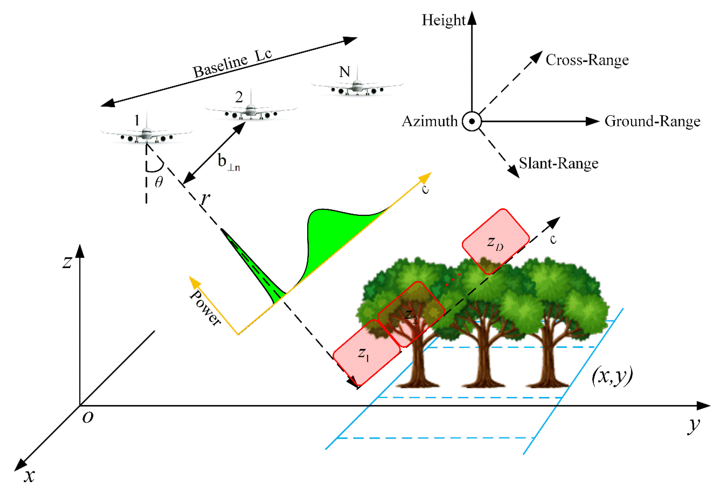
Figure 1.
Geometry and spectral estimation of the tomographic synthetic aperture radar (TomoSAR) configuration.
Figure 1.
Geometry and spectral estimation of the tomographic synthetic aperture radar (TomoSAR) configuration.
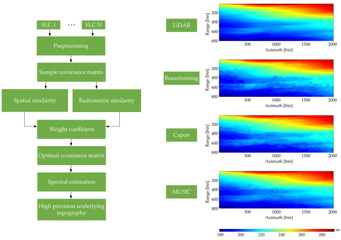
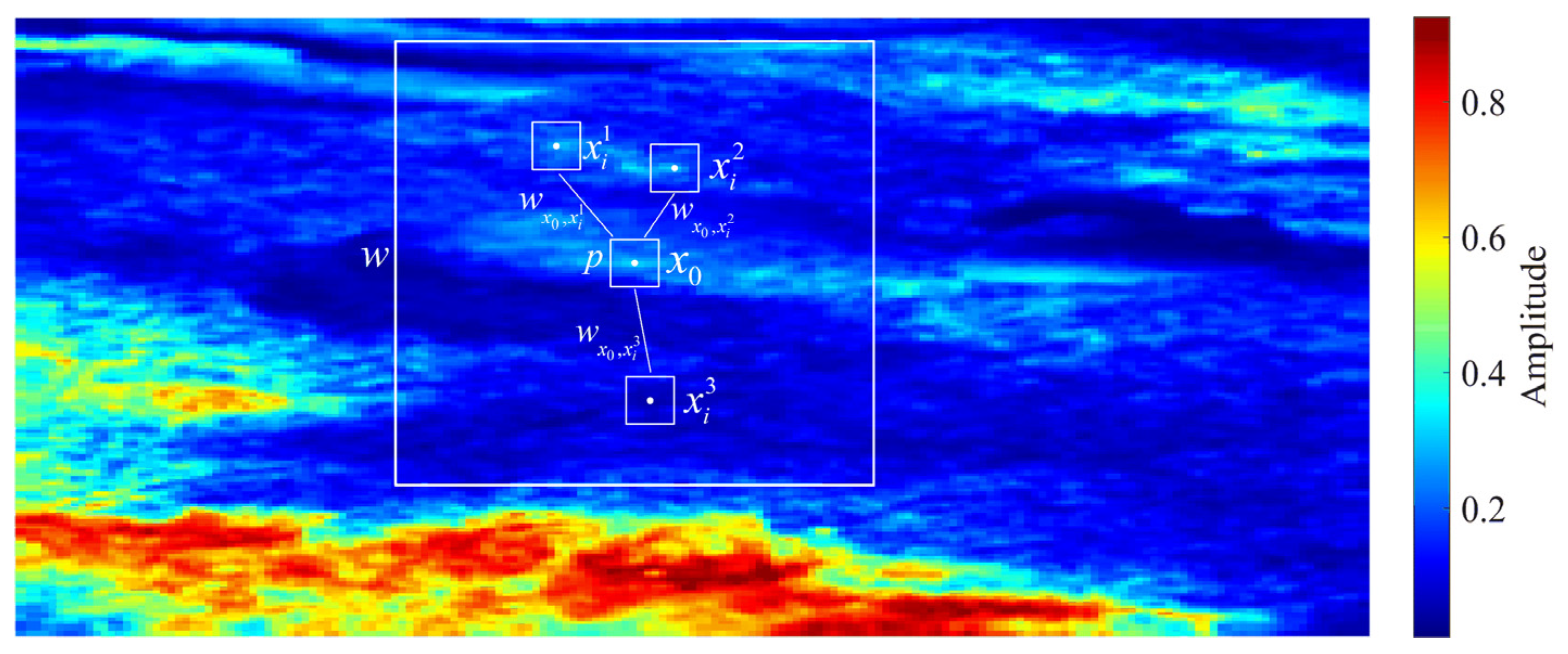
Figure 2.
The principle of optimal CM estimation based on NLM ( represents the size of the matching window, and denotes the size of the search window).
Figure 2.
The principle of optimal CM estimation based on NLM ( represents the size of the matching window, and denotes the size of the search window).
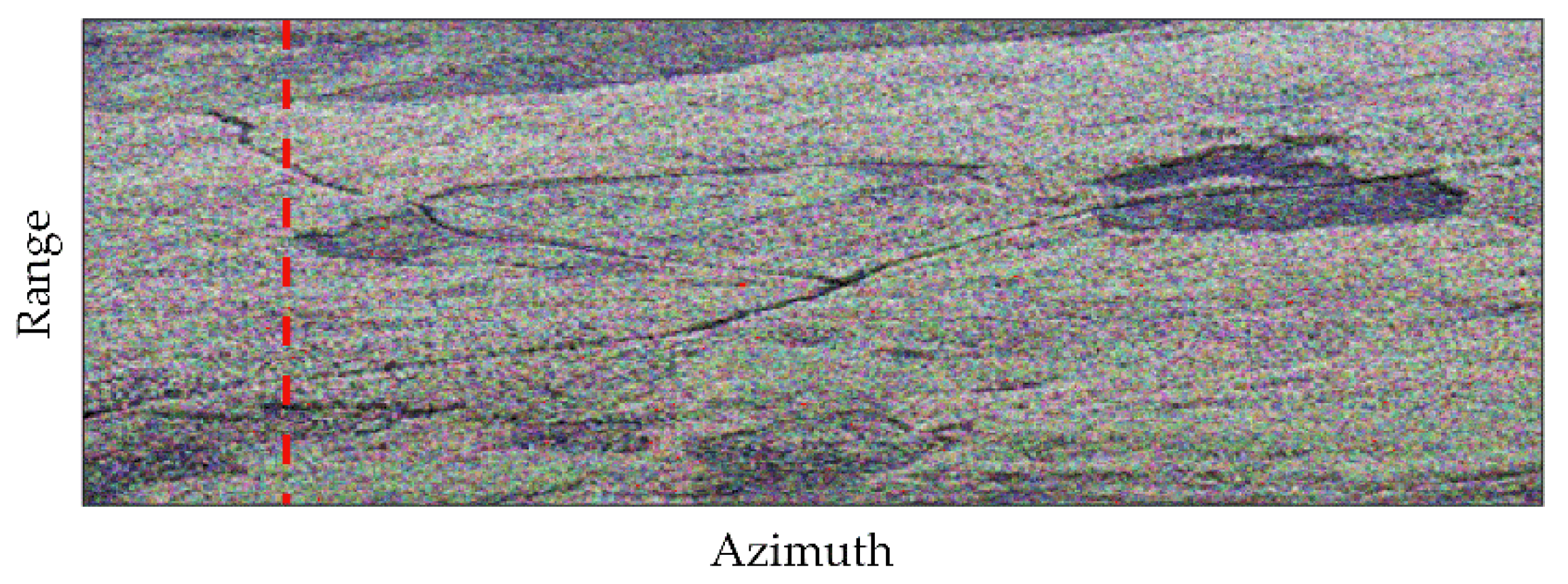
Figure 3.
The selected range profile (red dotted line) on the SAR Pauli map.
Figure 3.
The selected range profile (red dotted line) on the SAR Pauli map.
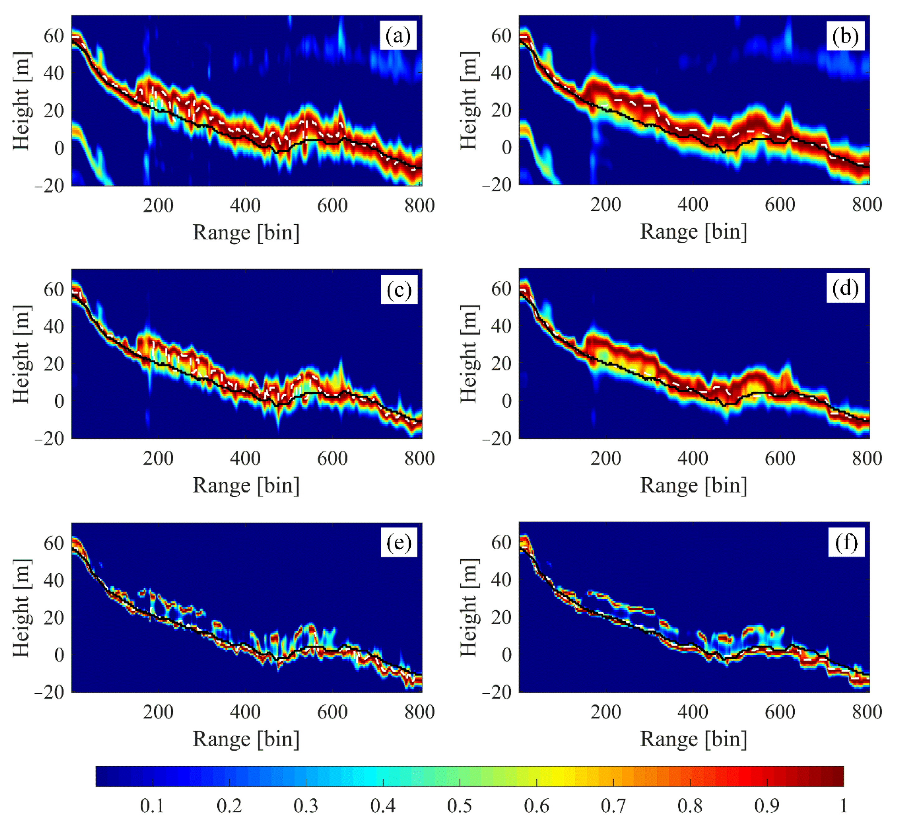
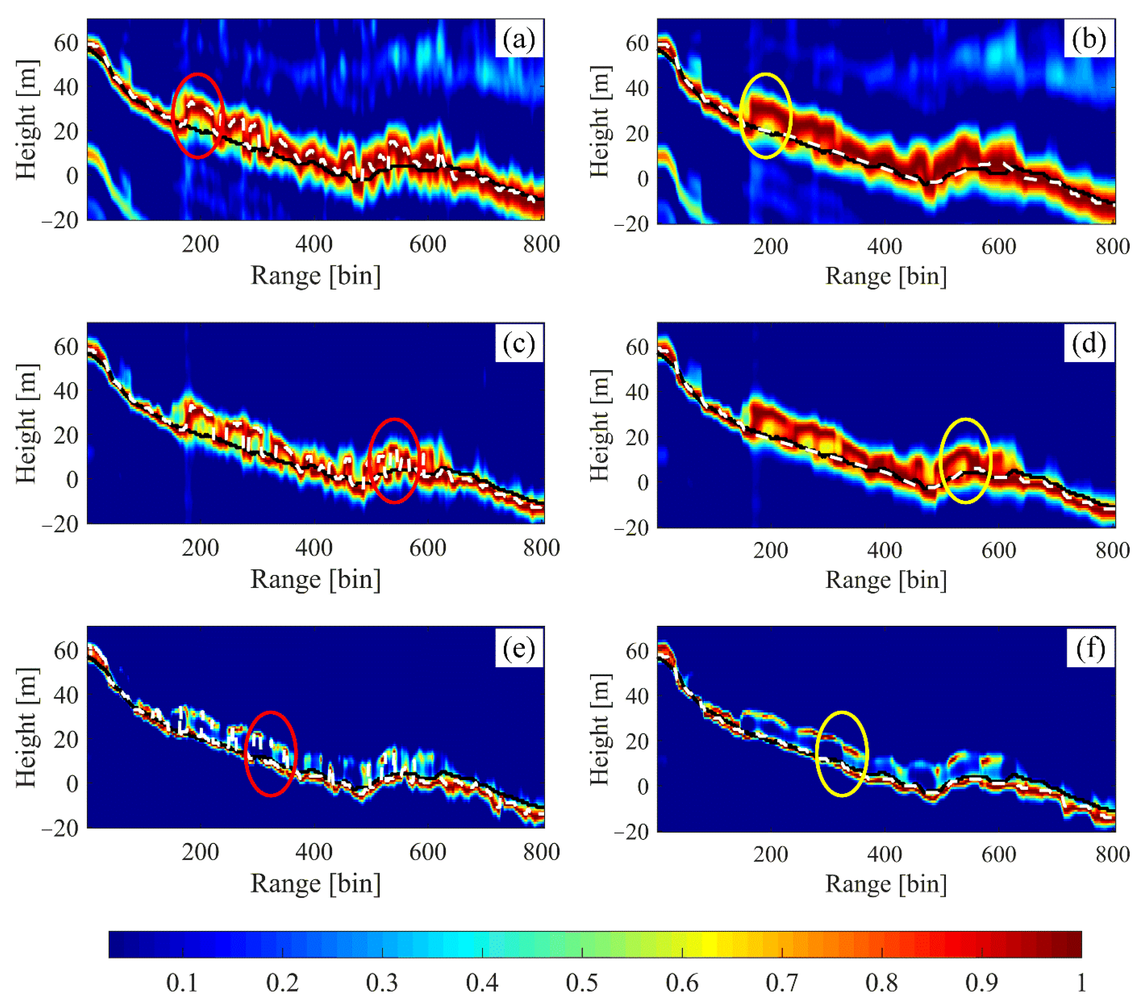
Figure 4.
Tomograms of the HH polarization channel at the selected profile estimated by the different TomoSAR methods: (a), (c), (e) are, respectively, the results of local means (LM)-based beamforming, adaptive beamforming (Capon), and multiple signal classification (MUSIC); and (b), (d), (f) are the results of NLM-based beamforming, Capon, and MUSIC, respectively. The solid black line is the LiDAR DTM, and the dashed white line is the estimated values.
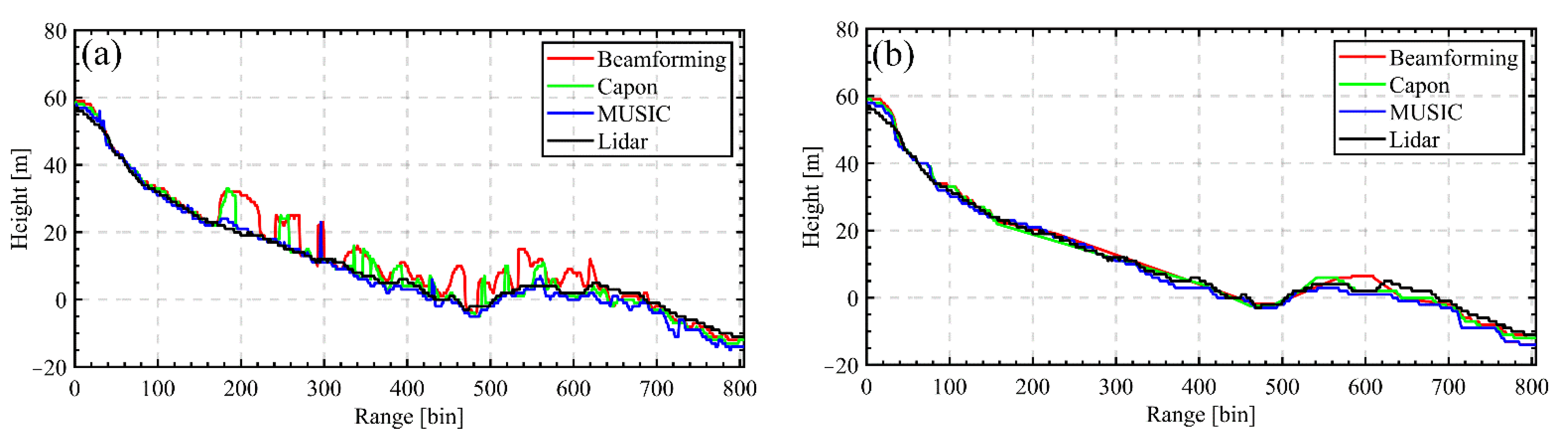
Figure 5.
The underlying topography at the selected profile: (a) the results of the LM-based TomoSAR method; and (b) the results of the NLM-based TomoSAR method.
Figure 5.
The underlying topography at the selected profile: (a) the results of the LM-based TomoSAR method; and (b) the results of the NLM-based TomoSAR method.
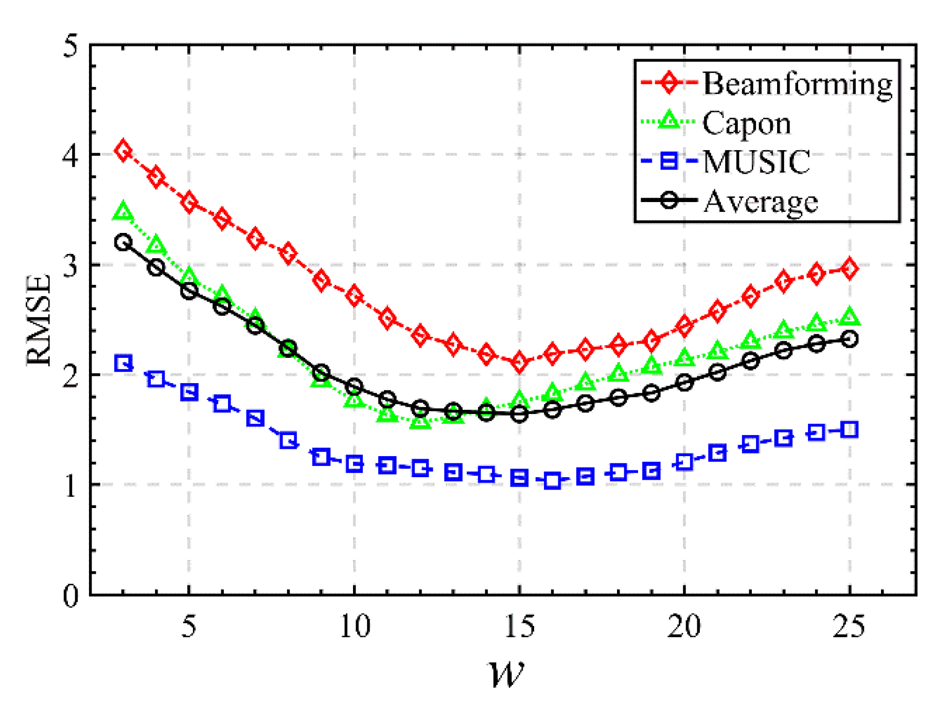
Figure 6.
The effect of the search window size on the RMSE.
Figure 6.
The effect of the search window size on the RMSE.
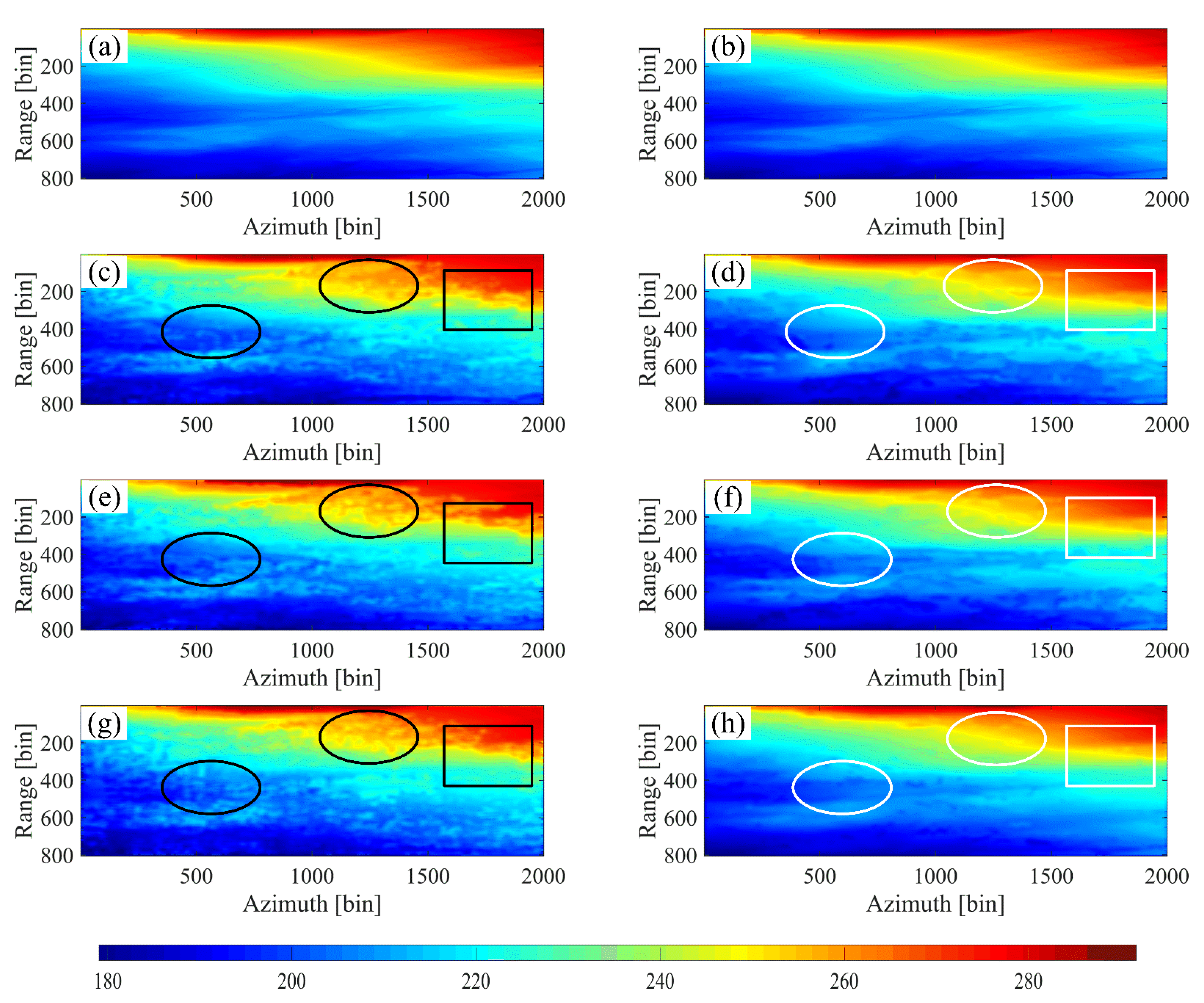
Figure 7.
Underlying topography from LiDAR and TomoSAR: (a,b) are the LiDAR DTM; (c), (e), (g) are, respectively, the beamforming, Capon, and MUSIC results based on the LM method; and (d), (f), (h) are, respectively, the beamforming, Capon, and MUSIC results based on the NLM method.
Figure 7.
Underlying topography from LiDAR and TomoSAR: (a,b) are the LiDAR DTM; (c), (e), (g) are, respectively, the beamforming, Capon, and MUSIC results based on the LM method; and (d), (f), (h) are, respectively, the beamforming, Capon, and MUSIC results based on the NLM method.
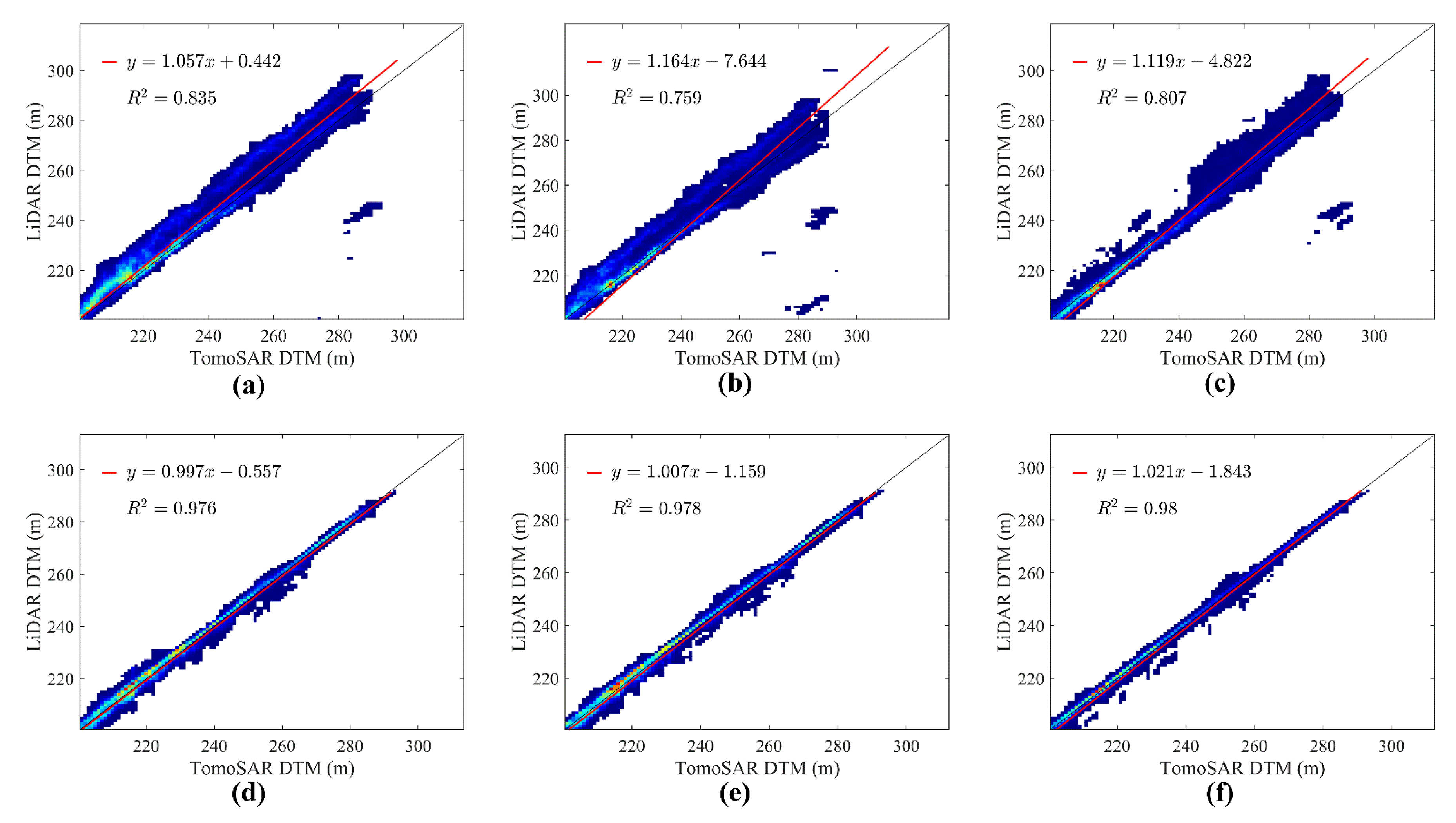
Figure 8.
The 2D joint distribution between the LiDAR and TomoSAR DTM of different methods: (a) LiDAR DTM and DM by LM beamforming; (b) LiDAR DTM and DTM by LM Capon; (c) LiDAR DTM and DTM by LM MUSIC; (d) LiDAR DTM and DTM by NLM beamforming; (e) LiDAR DTM and DTM by NLM Capon; (f) LiDAR DTM and DTM by NLM MUSIC.
Figure 9.
Comparison of the amplitude and phase of the CM for the different methods: (a), (c) are, respectively, the amplitude and phase of the CM of the LM method; and (b), (d) are, respectively, the amplitude and phase of the CM of the NLM method.
Figure 9.
Comparison of the amplitude and phase of the CM for the different methods: (a), (c) are, respectively, the amplitude and phase of the CM of the LM method; and (b), (d) are, respectively, the amplitude and phase of the CM of the NLM method.
Figure 10.
Tomograms of the HV polarization channel at the selected profile estimated by the different TomoSAR methods: (a), (c), and (e) are, respectively, the results of LM-based beamforming, Capon, and MUSIC; and (b), (d), (f) are, respectively, the results of NLM-based beamforming, Capon, and MUSIC. The solid black line is the LiDAR DTM, and the dashed white line is the estimated values.
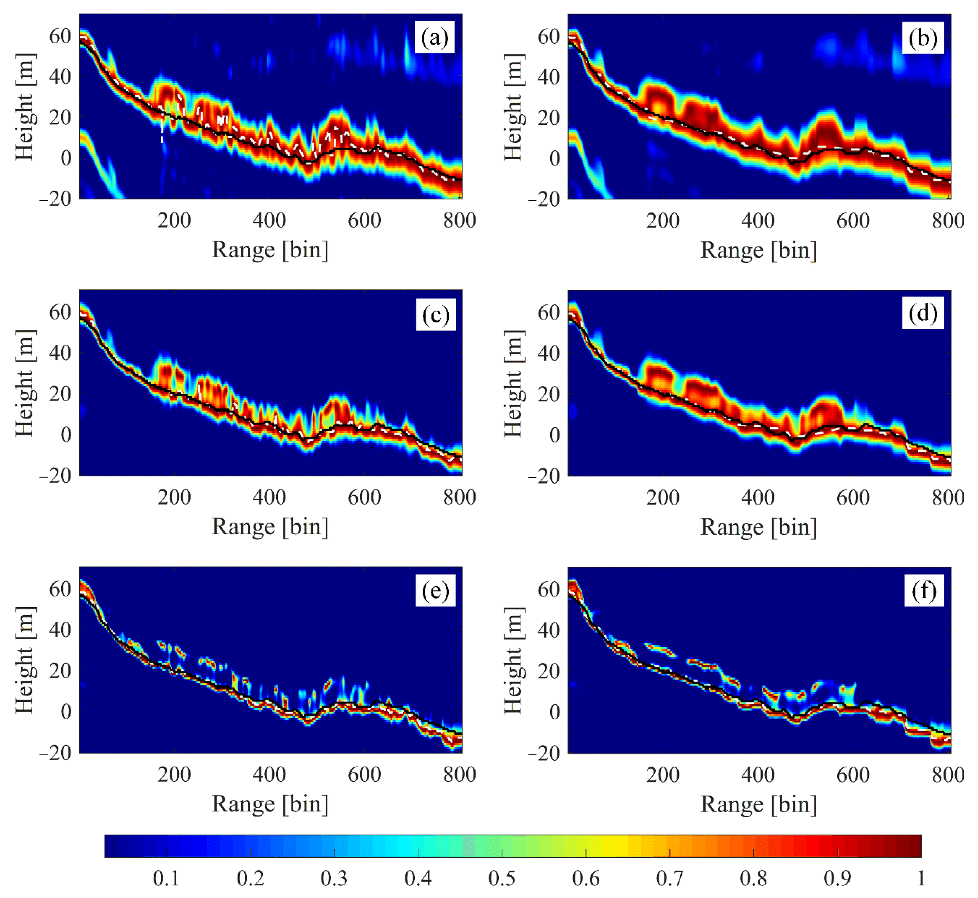
Figure 11.
Profile line spectrum estimation results for the VV polarization channel: the solid black line is the LiDAR DTM, and the dashed white line is the estimated values; (a), (c), and (e) are, respectively, the estimation results of LM-based beamforming, Capon, and MUSIC; and (b), (d), (f) are the estimation results of NLM-based beamforming, Capon, and MUSIC, respectively.
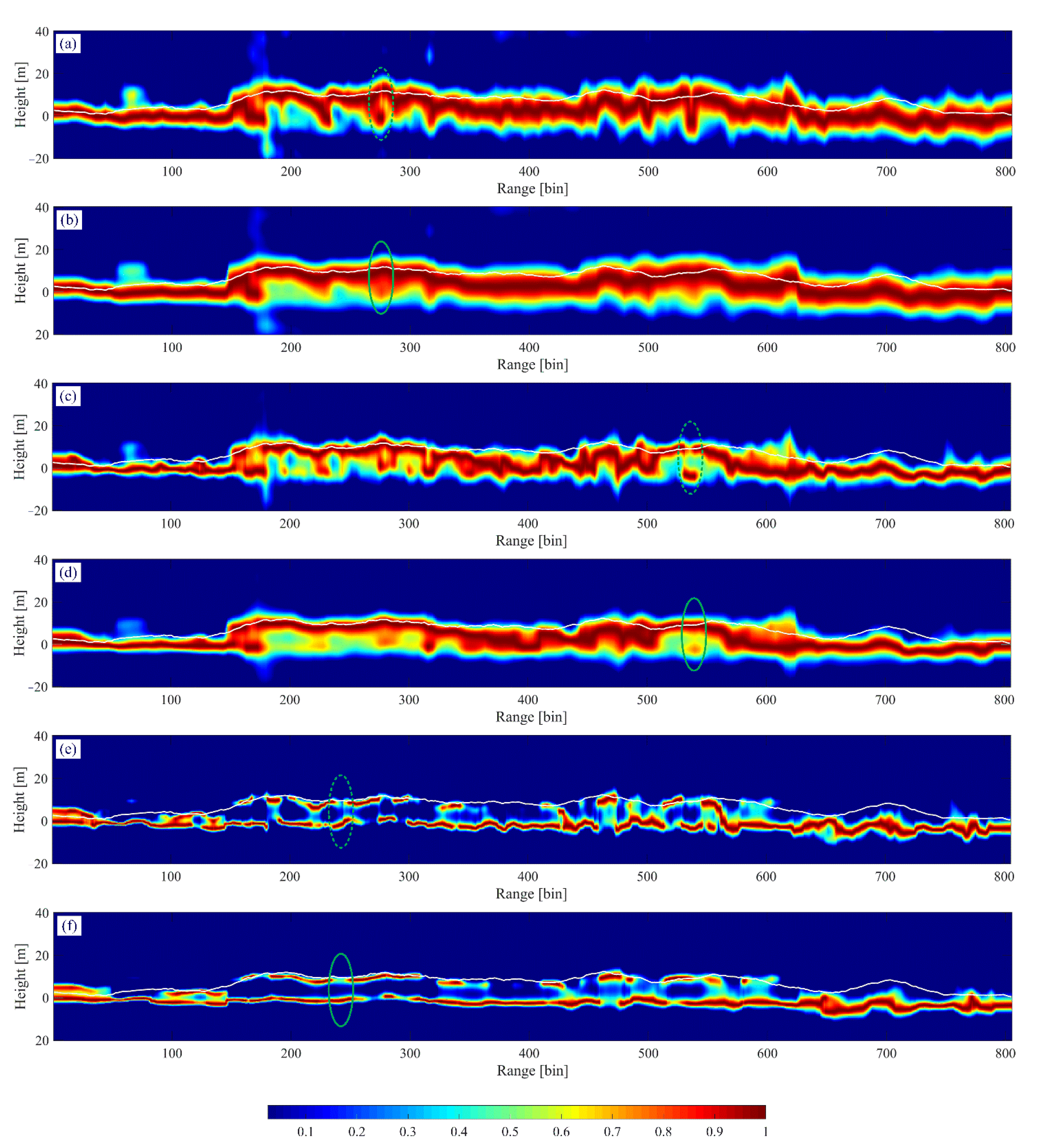
Figure 12.
Profile line spectrum estimation results for the HV polarization channel (terrain removed): the solid white line is the LiDAR canopy height model; (a), (c), and (e) are, respectively, the estimation results of LM-based beamforming, Capon, and MUSIC; and (b), (d), and (f) are the estimation results of NLM-based beamforming, Capon, and MUSIC.
Table 1.
Details of the classical spectral estimators based on NLM.
Table 1.
Details of the classical spectral estimators based on NLM.
| Initialization | |
| Traverse | |
| | repeat |
| | |
| | |
| | |
| | |
| | |
| Until (finish) | |
Table 2.
The parameters of the E-SAR airborne system [
40].
Table 2.
The parameters of the E-SAR airborne system [
40].
| Items | Parameters |
|---|
| Wavelength | 0.23 m (L-band) |
| Polarimetric channel | HH + HV + VV |
| Incidence angle | 25–55° |
| Center slant range | 3900 m |
| Range resolution | 2.12 m |
| Azimuth resolution | 1.20 m |
Table 3.
The baseline information for the InSAR pairs [
40].
Table 3.
The baseline information for the InSAR pairs [
40].
| Identifier | Acquisition Date | Baseline (m) |
|---|
| 08biosar0201 × 1 | 15 October 2008 | 0 |
| 08biosar0203 × 1 | −6 |
| 08biosar0205 × 1 | −12 |
| 08biosar0207 × 1 | −18 |
| 08biosar0209 × 1 | −24 |
| 08biosar0211 × 1 | −30 |
Table 4.
RMSE comparison of the different methods used for the profile analysis.
Table 4.
RMSE comparison of the different methods used for the profile analysis.
| Item | Beamforming (m) | Capon (m) | MUSIC (m) |
|---|
| LM | 3.24 | 2.87 | 1.55 |
| NLM | 2.11 | 1.77 | 1.06 |
| Improvement | 34.87% | 38.28% | 31.61% |
Table 5.
Running time of different methods.
Table 5.
Running time of different methods.
| Item | Beamforming (s) | Capon (s) | MUSIC (s) |
|---|
| LM | 26 | 25 | 24 |
| NLM | 369 | 371 | 374 |
Table 6.
Comparison of the RMSEs of the underlying topography inversion results.
Table 6.
Comparison of the RMSEs of the underlying topography inversion results.
| | Beamforming (m) | Capon (m) | MUSIC (m) |
|---|
| LM | 2.85 | 2.56 | 1.61 |
| NLM | 1.83 | 1.67 | 1.12 |
| Improvement | 35.78% | 34.76% | 30.43% |


 ,
, 


