
A Blended Sea Ice Concentration Product from AMSR2 and VIIRS


1
Cooperative Institute for Meteorological Satellite Studies, University of Wisconsin-Madison, 1225 West Dayton St., Madison, WI 53706, USA
2
Center for Satellite Applications and Research, NOAA/NESDIS, 1225 West Dayton St., Madison, WI 53706, USA
3
National Snow and Ice Data Center, CIRES, 449 UCB, University of Colorado Boulder, Boulder, CO 80309, USA
*
Author to whom correspondence should be addressed.
Remote Sens. 2021, 13(15), 2982; https://0-doi-org.brum.beds.ac.uk/10.3390/rs13152982
Submission received: 5 May 2021
/
Revised: 20 July 2021
/
Accepted: 22 July 2021
/
Published: 29 July 2021
(This article belongs to the Special Issue Polar Sea Ice: Detection, Monitoring and Modeling)
Abstract
:An effective blended Sea-Ice Concentration (SIC) product has been developed that utilizes ice concentrations from passive microwave and visible/infrared satellite instruments, specifically the Advanced Microwave Scanning Radiometer-2 (AMSR2) and the Visible Infrared Imaging Radiometer Suite (VIIRS). The blending takes advantage of the all-sky capability of the AMSR2 sensor and the high spatial resolution of VIIRS, though it utilizes only the clear sky characteristics of VIIRS. After both VIIRS and AMSR2 images are remapped to a 1 km EASE-Grid version 2, a Best Linear Unbiased Estimator (BLUE) method is used to combine the AMSR2 and VIIRS SIC for a blended product at 1 km resolution under clear-sky conditions. Under cloudy-sky conditions the AMSR2 SIC with bias correction is used. For validation, high spatial resolution Landsat data are collocated with VIIRS and AMSR2 from 1 February 2017 to 31 October 2019. Bias, standard deviation, and root mean squared errors are calculated for the SICs of VIIRS, AMSR2, and the blended field. The blended SIC outperforms the individual VIIRS and AMSR2 SICs. The higher spatial resolution VIIRS data provide beneficial information to improve upon AMSR2 SIC under clear-sky conditions, especially during the summer melt season, as the AMSR2 SIC has a consistent negative bias near and above the melting point.
1. Introduction
Sea-Ice Concentration (SIC) is the fraction of the sea surface covered by ice over some area, typically the satellite field of view (pixel). SIC is important in applications such as marine transportation, coastal erosion and its prevention, natural resource exploration, fisheries, subsistence hunting, and wildlife management and research. Sea ice influences the surface energy budgets and moisture exchange between the atmosphere and the underlying water. Thus, it is a key factor in atmospheric and oceanic circulation and is an essential component for numerical weather forecasting and climate modeling. Over the past few decades, Arctic sea ice has changed dramatically with decreases in sea ice extent [1], coverage [2], and volume [3]. These changes are associated with rapid increasing surface temperatures [4], heat [5], and moisture fluxes [6] and decreasing surface albedo [7], and changes in cloud properties [7] and atmospheric stability [8] in the Arctic. Arctic climate change is potentially connected to midlatitude changes through shifting global scale jet stream patterns, resulting in more extreme weather events [9,10,11].
Due to the remote and harsh conditions over the sea ice, ground-based observations of the SIC are extremely limited. With their high spatial and temporal coverage over the polar regions, polar-orbiting satellites have been crucial in observing changes in Arctic sea ice for more than four decades. Satellite observations utilizing the microwave portion of the electromagnetic spectrum can provide the SIC under all weather (clear and cloudy-sky) conditions. A recent and widely used passive microwave satellite is the Japan Aerospace eXploration Agency (JAXA) Global Change Observation Mission–Water (GCOM-W) carrying the Advanced Microwave Scanning Radiometer 2 (AMSR2) instrument. Several sea ice algorithms, such as the NASA Team (NT) algorithm, the enhanced NT algorithm (NASA Team-2), the Bootstrap (BS) algorithm, and the ARTIST Sea Ice (ASI) algorithm, have been used to estimate the SIC. More specific details on these types of sea-ice-derived products are given in [12,13,14,15,16]. Another type of satellite instrument that has been used in observing the sea ice utilizes the visible and infrared (IR) portions of the electromagnetic spectrum. SIC products have been generated for visible/IR imagers, such as the Advanced Very High Resolution Radiometer (AVHRR), the Moderate Resolution Imaging Spectroradiometer (MODIS), and the Visible Infrared Imaging Radiometer Suite (VIIRS). More details on the sea ice products derived from VIIRS are given in [17,18,19,20,21,22].
While passive microwave instruments provide sea ice information under all-weather conditions, they do so with relatively low spatial resolution, for example, 10 km for NASA Team-2 [23,24] and 6.25 km for the ASI algorithm [25]. For this study, SIC products based on the NASA Team-2 algorithm utilizing the 18, 36 and 89 GHz channels are used [16]. While AVHRR, MODIS, and VIIRS SIC products are only for clear-sky conditions, these products provide information at a higher spatial resolution, up to 0.375 km for VIIRS. With emerging weather and climate models that have sub-kilometer grid spacing [26,27], boundary layer conditions with 1 km and sub-kilometer resolutions may be needed. Such high spatial resolution SIC products are also key in the study of processes with small spatial scales such as sea ice leads (fractures), and are relevant to operational analyses supporting navigation and other activities in sea ice regions [28]. Previous work has been undertaken in optimizing different passive microwave SIC retrievals [29] and combining visible and thermal infrared MODIS SIC with passive microwave AMSR2 SIC [30]. The combined satellite product discussed in [29] has been shown to have particularly good agreement with other SIC products and independent sea-ice cover data [31].
In this paper we present a new, high spatial resolution SIC product for all-weather conditions through an optimal blending of the SIC products from AMSR2 and VIIRS. We use the Best Linear Unbiased Estimator (BLUE) method to combine sea ice products from the all-sky, lower spatial resolution AMSR2 and the clear-sky, higher spatial resolution VIIRS for a blended SIC product. Landsat 8 data are employed to perform a validation of the individual AMSR2 and VIIRS SIC, and the blended fields. Qualitative comparisons to natural color Sentinel-2 images and Sentinel-1 Synthetic Aperture Radar (SAR) for individual cases are shown. Special attention is paid to the quality of these products in melting sea ice environments. Our product differs from Ludwig et al. [30] in the blending methodology and in the seasonal applicability. More details of the differences are in Section 4. The blended SIC product presented here has been routinely generated at the National Oceanic and Atmospheric Administration (NOAA)/University of Wisconsin—Madison Cooperative Institute for Meteorological Satellite Studies (CIMSS) since 2018. While it is currently a research product, validation results indicate that it can be a viable operational, near-real-time product.
2. Data and Method
An algorithm has been developed to detect ice and estimate SIC in clear-sky areas over the ocean and inland lakes and rivers using VIIRS [18] on board the S-NPP and NOAA-20 satellites. A threshold method is used to discriminate between ice and open water. A tie-point algorithm is then applied to determine the representative visible reflectance (daytime) or ice surface temperature (nighttime) of the pure ice cover at the center of a sliding search window with a size of 50 by 50 km. SIC at the center of the search window is then retrieved from its observed reflectance/ice surface temperature [18]. This product has a spatial resolution of 750 m, the spatial resolution of the VIIRS’s moderate resolution bands. An example of a daily composite of VIIRS SIC over the Arctic remapped to 1 km grid is shown in Figure 1a. The clear/cloudy conditions are determined by the cloud mask derived from the VIIRS M-band data. Only confidently clear pixels are used in SIC estimates to limit the effect of cloud contamination. We use the NASA Team 2 algorithm to retrieve SIC with AMSR2 [32], which provides estimates in all-weather conditions (Figure 1b). Their spatial resolutions are relatively coarse—10 km EASE Grid version 2 resolution [33,34]. The uncertainties of passive microwave SIC of up to 20% are relatively larger over regions where there are rapid changes over short spatial and temporal scales, such as the marginal ice zones, coastal areas, regions of melting and freeze-up, over thin ice and melt ponds, and some ice features in the pack ice such as leads and floes [35,36,37,38]. Visible data are likely to produce more accurate summer daylight SIC, because similar microwave emissivities of melting snow/ice, melt ponds on the ice, and open water result in large biases and uncertainties in the passive microwave estimates [32]. However, as with all visible and infrared sensors, the VIIRS SIC is only available under clear-sky conditions.
A total of 1486 Landsat scenes over the Arctic Ocean from 2017 to 2019 were collected and collocated with VIIRS. These scenes are only daylight and therefore primarily from late March through early October with highest density of scenes coming from the well sunlit summer months of June through August. These scenes are throughout the Arctic and confined to areas that are usually within 500 km of a landmass that includes islands. A Landsat scene is selected if over 90% of all pixels are clear based on Landsat’s own cloud mask [39]. All the selected scenes are then manually inspected by Arctic cloud detection experts, the authors, to remove those scenes, in which clouds are not detected by its own cloud mask. The original spatial resolutions of Landsat and VIIRS are 30 m and 750 m, respectively. For each Landsat scene, visible and thermal channel observations at 30 m spatial resolution are available from the Operational Land Imager (OLI) and the Thermal Infrared Sensor (TIRS). Only daytime images are used because of more spectral information (shortwave channels) and thus higher confidence in the ice identification during the daytime and possibly better cloud detection from both VIIRS and Landsat. Each Landsat clear-sky pixel determined from Landsat’s cloud mask [39] is identified as ice if the normalized difference snow index (NDSI), calculated from band 5 (0.865 μm) and band 6 (1.6 μm), is larger than 0.45, and if the reflectance at band 5 is higher than 0.08 [18]. Landsat SIC is at the 1 km spatial grid, the same as the remapped VIIRS. This was calculated as the ratio of the number of 30 m Landsat ice pixels to the total number of pixels in a 1 km grid cell. Of the 1486 scenes, 484 scenes or a 31% subset are used to derive the measurement accuracies and precisions of the collocated VIIRS and AMSR2 SIC, and the rest are used for independent validation.
We here present a blending approach to optimize all-weather SIC and ice cover estimates from passive microwave observations (AMSR2) and clear-sky SIC and cover with very high spatial resolution from visible/infrared observation (VIIRS) to monitor the ice characteristics effectively under all-weather conditions. The combined use of the SIC from these two products requires uncertainty estimates for both products compared to a reference dataset and a robust scheme to combine them. Here, we use SIC derived from high-resolution Landsat 8 data [40] (hereinafter simply “Landsat”) as the reference “ground truth”. Uncertainties in the AMSR2 and VIIRS SIC are expressed as the bias (mean difference, also called the accuracy) and standard deviation (precision) of the differences between the AMSR2 or VIIRS and Landsat SIC. Before the blending, the AMSR2 and VIIRS SIC products are remapped to a 1 km EASE Grid version 2 using a nearest neighbor approach.
Under clear-sky conditions, the Best Linear Unbiased Estimator (BLUE) method [41] is applied to derive the combined final SIC:
where Cclear, CA, and CV, are blended SIC, and retrieved SIC from AMSR2 and VIIRS, respectively; DA and DV are measurement bias between the AMSR2 or VIIRS SIC and the Landsat SIC (Figure 2); σA and σV are the standard deviations of the differences. For the pixels under cloudy conditions, the blended SIC is determined as the SIC from the passive microwave observations with a bias correction. The correction is defined as the retrieved (observed) AMSR2 SIC minus a bias. The bias is determined through linear interpolation between the observed SIC and the previously determined bias of the bin into which the observed SIC falls:
where CA is the retrieved AMSR2 SIC, D is a bias lookup table for a particular SIC bin and a particular surface temperature range, with xs being the midpoint value inside the SIC bin. For brevity, 20% intervals are shown from 30 to 90% in Figure 2. The Gaussian fits are included to show which ranges would work best with the BLUE method. In general, according to the figure distributions, anything above 50% for AMSR and 30% for VIIRS should work well in the BLUE.
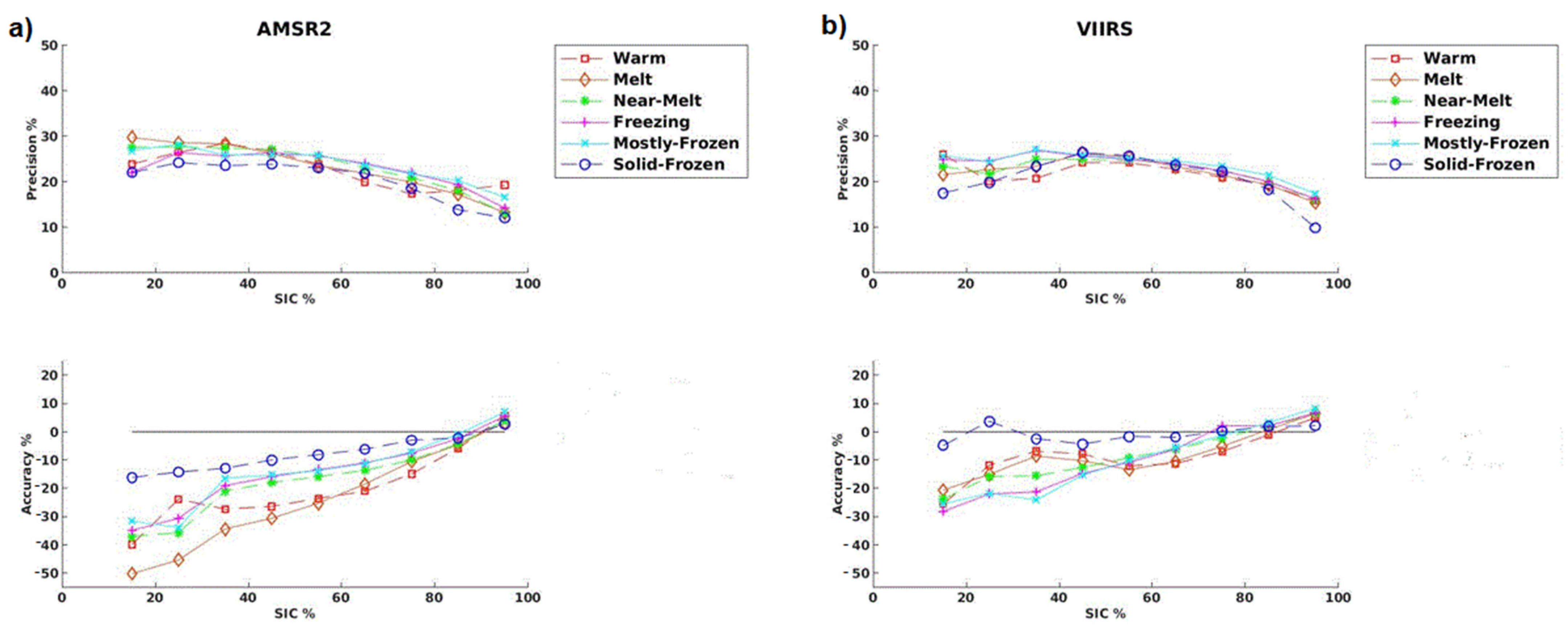
Measurement precision (standard deviation) and accuracy (bias) of AMSR2 (Figure 2a) and VIIRS (Figure 2b) SIC compared to Landsat are calculated for different SIC bins from 0–100%, with lookup tables dependent upon VIIRS and AMSR2 SIC and the VIIRS Ice Surface Temperature (IST) (Table 1). The surface temperature information is used to account for the dependence of SIC quality on ice surface conditions, especially for passive microwave SIC in clear-sky conditions, which are shown in six separate precision and accuracy tables (see Table 1a–f and Figure 3). The six tables are in one-degree increments starting from 270.15 K to 274.15 K. Surface temperature above 275 K is considered to be unfrozen water. In Table 1, the temperature bins further below the freezing point of water are applied to account for increased salinity values of ocean water that decrease the actual freezing point temperature of water. In addition, due to a negative skew observed in the AMSR2 SIC product compared to Landsat for SIC less than 70% (Figure 2a), the VIIRS SIC with bias correction is only used when SIC differences between AMSR2 and VIIRS are greater than a certain threshold, set to 20% based on independent comparisons to Landsat between VIIRS and AMSR2 and when AMSR2 SIC is less than 70% for IST near or above melting (272.15 ≤ K). This is performed because larger difference between these two values indicates that one of these retrievals is substantially less accurate, and it is shown that is likely to be AMSR2 when the SIC is low and in near-melting or melting environments. Furthermore, VIIRS SIC product comparison to Landsat showing limited skewness and a more normal distribution suggests better retrieval of VIIRS SIC (Figure 2b). Otherwise, if these thresholds are not included it would introduce a negative bias to the final blended product. Results will show that this method works well and improves SIC quality over the Arctic.
An example of blended VIIRS-AMSR2 SIC is shown in Figure 1c, which clearly illustrates the significant amount of detail that is provided by the VIIRS SIC product in various localized regions, for example off the northern and northeast coasts of Greenland including the Wandel and Lincoln Seas. For the blended SIC, ice cover is defined by pixels with SIC larger than a certain threshold, which is set to 15%, with anything lower than that value set zero SIC. The final product has the same spatial resolution as remapped VIIRS into EASE2 grid at 1 km, with microwave observations interpolated onto the same grid spatial resolution with a bias correction in regions of cloud cover. The effective resolution of the blended product lies between 1 km and 10 km, depending on the relative precision, e.g., the weights of AMSR2 and VIIRS in the blended product as expressed in Equation (1). In some conditions, such as in near-melt or melting environments when AMSR2 SIC less than 80% and SIC difference between AMSR2 and VIIRS greater than 20%, the final blended SIC defaults to VIIRS, and the effective resolution will be 1 km. Additionally, as noted, in cloudy conditions, when VIIRS is not available, the effective resolution becomes 10 km, the same as the AMSR2 resolution.
3. Results
In this section, a case study comparing Landsat SIC to AMSR2, VIIRS, and blended SIC will be shown, including a robust quantitative analysis of the similarities and differences between the products. Next, a Sentinel-2 multispectral image in a melting sea ice environment will be compared to the SIC products. VIIRS ice surface temperature is then used to investigate the performance of the individual and blended SIC products in melt conditions. In the Discussion section, two winter scenes will be qualitatively compared to Synthetic Aperture Radar (SAR) and 4-km daily SIC from the blending of AMSR2 NASA Team-2 SIC and the Multisensor Analyzed Sea Ice Extent (MASAM2) product to demonstrate the potential quality of the blended SIC product in the dark winter conditions, with further discussion on how to improve the blended SIC from this point forward.
3.1. Case Study
First, we show the results of a regional case study, comparison between AMSR2, VIIRS, and the blended SIC versus Landsat SIC over the Fram Strait (between Svalbard and Greenland) and the Wandel Sea (northeast of Greenland and north of the Fram Strait) on 1 August 2019 (Figure 4 and Figure 5). The results from this primarily cloud-free scene show the ability of the blended product to improve upon the all-weather AMSR2 product by resolving smaller features in the ice field, such as large ice floes and a more detailed ice edge. Specifically, the large floe features in the VIIRS SIC off the coast of Greenland and in the Fram Strait are retained by the blended product, for example the rectangle region in Figure 5b. Additionally, SIC is improved in heterogeneous pockets over the interior pack ice over the Fram Strait in the northeast quadrant (circle region in Figure 5c) where it is underestimated by VIIRS. The areas where the blended SIC diverges from Landsat are the northernmost region of the Wandel Sea (oval region in Figure 5e), near the immediate coastline of Greenland, and along the northern ice edge with the southeast ice field (oval in Figure 5b), where the blended product overestimates sea ice due to VIIRS cloud masking and overestimation by AMSR2. The differences from Landsat and the blended product could be the result of rapid melt and ice deterioration between VIIRS overpasses and Landsat, and that the VIIRS overpass closest in time (36 min) to Landsat was at the swath edge where smaller scale features in the field are smeared by the sensor bow-tie correction [42]. Furthermore, the visible/IR ice product can only be as good as the cloud mask, and as an example, if the cloud mask is too passive in cloud detection, that will lead to an overestimation of sea ice with misidentification of undetected ice cloud as sea-ice cover. Another influence could be ice drift and assuming ice moves at 5 cm/s, and 1 h time difference means 180 m spatial distance between the scenes from two satellites [43]. The best measure of how the blended product performs is a quantitative analysis (Figure 6). The quantitative comparison for this scene indicates improved bias, standard deviation of differences, and Root Mean Square (RMS) difference statistics of the blended product versus the estimates from the individual AMSR2 and VIIRS sensors when compared to Landsat SIC. AMSR2 has a negative bias while VIIRS has a positive bias of about the same magnitude of a little over 5%. The AMSR2 bias is the result of underestimation of the SIC associated with large ice floes and along the sea ice edge and marginal ice zone. The positive bias of VIIRS is the result of overestimation SIC in the northwest marginal ice zone (Figure 5e) and heterogenous areas of the pack ice (Figure 5c). Overall, the VIIRS SIC produces a higher frequency of zero bias compared to both AMSR2 and blend. To determine the significance of the blended product superiority to VIIRS and AMSR2, a much larger sample size of cases is required. An analysis of a much larger sample size is the topic of the next section.
3.2. Comparison to Landsat 8
An analysis of SIC between VIIRS, AMSR2, the blended, and Landsat SIC for multiple days from 2017 to 2019 was completed for this study (Figure 7). Over this period, any differences of greater than 20% between the blended and either the AMSR2 or VIIRS SIC were cataloged and compared to Landsat-derived SIC (if available for that day). Overall, a total of 1002 Landsat scenes remapped into 1 km EASE2 grid cells that were not used in training blending model, Equations (1) and (2), were compared to the blend, AMSR2 and VIIRS. These scenes were determined to be mainly clear and during daylight. Difference distribution histograms compared to Landsat are shown in Figure 7. For a total of 9,666,807 collocated 1 km grid cells, the blended product produces the lowest standard deviation and RMS errors during daylight conditions compared to Landsat. Due to the independent Landsat dataset being limited to daylight conditions, the quality of dark winter conditions is unknown at this time. Furthermore, AMSR2 has the lowest bias, but the largest standard deviation error. On the other hand, the blended SIC product significantly reduces the standard deviation of the errors of AMSR2 SIC while also reducing the VIIRS positive bias. However, even with improved statistics, the blended SIC product has a slightly negative skew with a local maximum at around −8% and retained long positive tail. The negative skew is caused by the non-normalized asymmetric distribution of the AMSR2 SIC compared to the reference dataset, and the positive tail is hypothesized to be due to ice cloud contamination in VIIRS and the positive tail of AMSR2 in coastal sea ice, which will be shown later. It is expected that the positive tail will be mitigated with the planned migration to an improved, “enterprise”, cloud mask that utilizes Bayes’ theorem and includes cloud probabilities, thereby allowing for fine tuning of the cloud mask settings [44]. A further discussion of how to reduce the skew and positive tail of the distribution of differences is given in the summary and conclusion section.
3.3. Melting Ice Conditions
Next we investigate the performance of the product under melting ice conditions, which is a significant contributor to the differences observed between VIIRS and AMSR2 SIC values. Figure 8 (see Figure 4 for location) shows a case study over the southern Hudson Bay on 18 June 2018. In this case there is significant melting of the sea ice as determined by VIIRS IST values near and above the melting point. AMSR2 SIC over the region is predominantly in the range of 80–90%, while VIIRS produces SIC in the range of 90–100%, or 10–20% higher than AMSR2. The blended SIC retains many of the features present in the VIIRS SIC with overall SIC around 90%. The Sentinel-2 Multi-Spectral Instrument Level-1C data (S2MSI1C) composite for the same day and close proximity in time (60 min) indicates dense sea-ice coverage 50–100 km from the south coast of Hudson Bay. Qualitatively, it appears that AMSR2 underestimates the sea-ice coverage while VIIRS and blended SIC matches more closely to what is seen in the Sentinel-2 image. However, one issue with the blended SIC in this case is that it overestimates the SIC near the coast because of the widespread ice coverage present in the AMSR2 product, where the VIIRS cloud mask seems to be too conservative in flagging water grid cells as cloud-covered. It has been shown that in comparison to the Interactive Multisensor Snow and Ice Mapping System (IMS), AMSR2 tends to overestimate sea ice near coastlines [45]. AMSR2 can overestimate SIC near the coast due to coastal contamination, i.e., ocean grid cells containing sensor footprints that overlap the coast and have emission from both ocean and land. Generally, the overestimate in SIC is retrieving a non-zero concentration where no ice exists. The mixture of ice-free ocean and land has a signature similar to sea ice. A land-spillover filter removes some of this false ice, but not all of it.
For quantitative analysis, a similar period detailed in Section 3.2 is processed by comparing AMSR2 and VIIRS SIC over an IST range starting from 230 to 275 K (Figure 9). First, AMSR2 has a consistent negative difference of 1 to 2% compared to VIIRS due to VIIRS producing sharper SIC gradients along the sea ice edge and the inability of AMSR2 to resolve small feature such as floes and leads in the pack ice. Most notably, it shows the rapid drop in the bias of AMSR2 SIC compared to VIIRS for IST starting at 272 K with a bias of +2% to 275 K with a bias of −8%. As the ice deforms in melting environments, surface water contamination leads to underestimation of the AMSR2 SIC [24,45,46]. The sharp rise in bias from −2% to +2% as IST approaches 270 K will require additional investigation, though it is hypothesized that it is due to the freeze-up condition and the formation of new grey ice that would be underestimated by VIIRS in NDSI calculation [20,47].
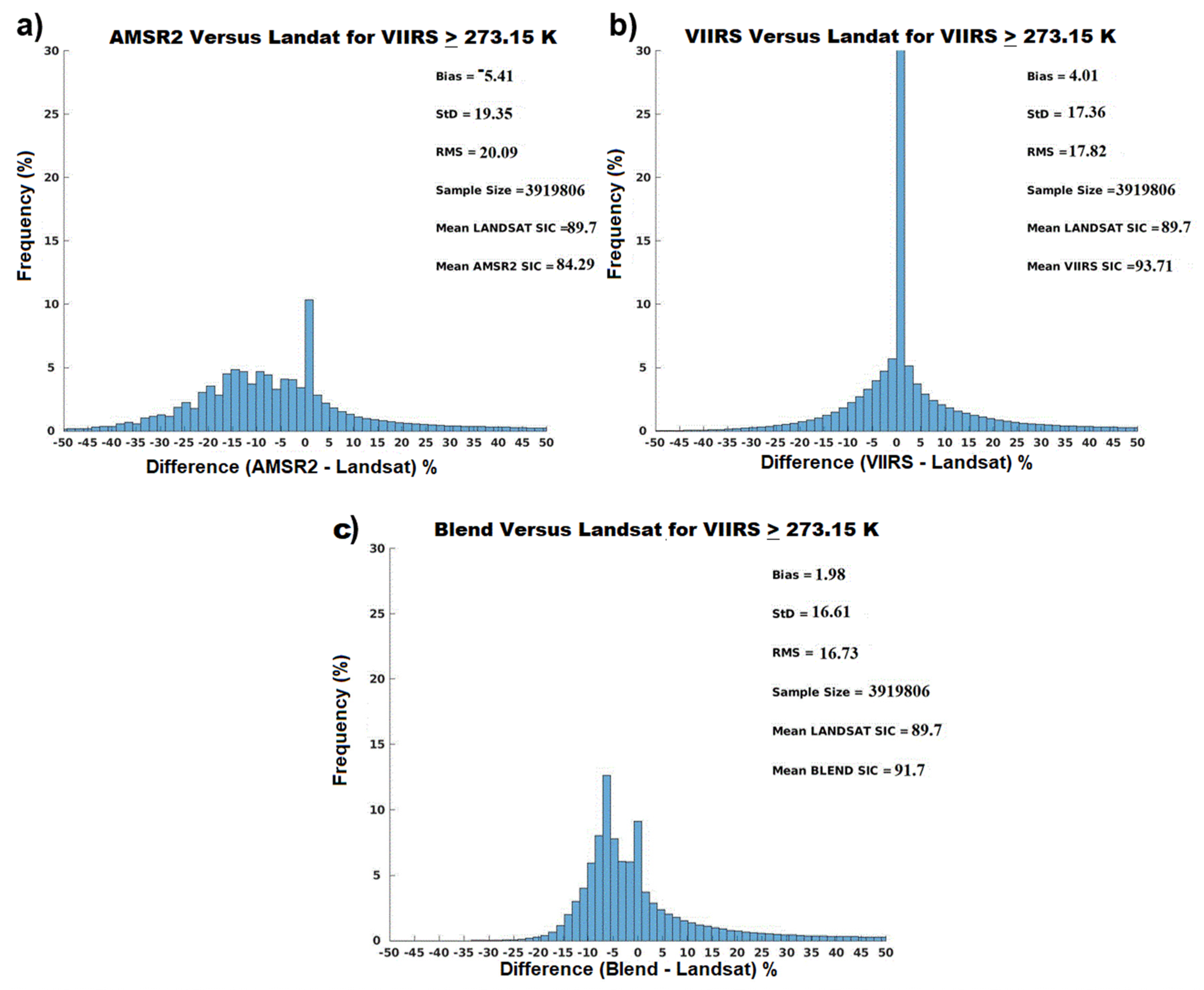
Finally, histogram difference distribution plots in Figure 10 show all cases where the VIIRS IST is at or above the melting point. The AMSR2 SIC in these conditions have a significant negative skew compared to Landsat, while VIIRS SIC has a Gaussian distribution. The final blended SIC product produces the overall lowest bias, standard deviation and RMS differences compared to Landsat. However, the final blended SIC does have a negative skew that is maximum at −7%. Even so, it still outperforms the individual AMSR2 and VIIRS products in error measurements.
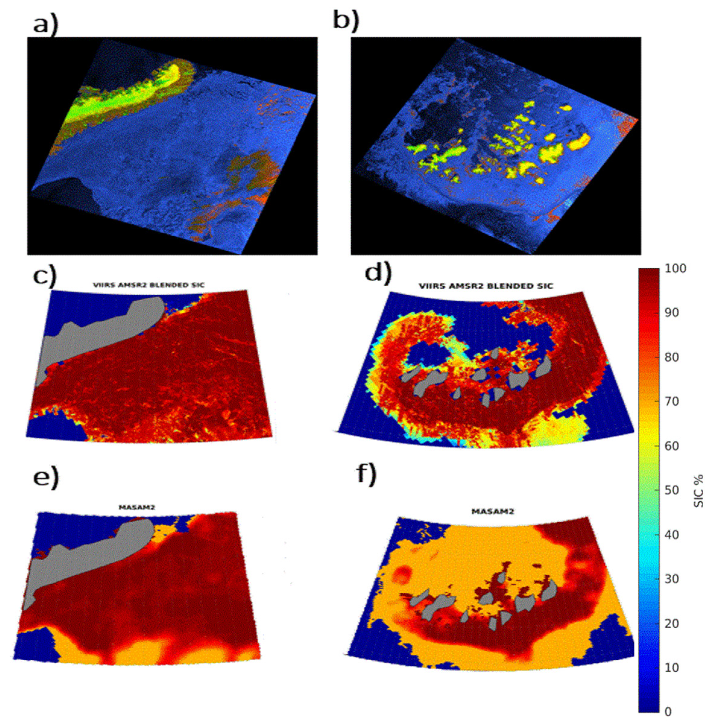
4. Discussion
There is the potential for further improvements to the blended concentration product. First, more in-depth investigation of the product during the winter season utilizing SAR on the Sentinel-1 satellite is feasible [48]. Unfortunately, at the present time the lack of an available operational SAR SIC product makes validation in the dark winter season limited to qualitative comparison with level 1B HH + HV polarization imagery, as shown in Figure 11 (see Figure 4 for locations). Compared to the MASAM2 SIC product [49] from the same day, the blended shows more detail over the pack ice with sharper gradients at the sea ice edge with blended (MASAM2) having more higher (medium) range SIC. Once a reliable SAR SIC product becomes available then a quantitative analysis can be performed. Furthermore, it will be possible to include SAR SIC into the final blended product.
In this study, validation focused on the Arctic melt season (March–September), with limited cases from the initial freeze-up season (October–November). In future work, we will focus on the early freeze-up season cases that are available during the limited sunlit days of late September into October and early November. This will allow for additional evaluation of accuracy and precision for near-melt or near-freeze conditions to be used in the BLUE for the freeze-up season.
Next, more comparisons to Landsat in areas of coastal ice (within 50 km of the coastline) is necessary to build a separate lookup table of accuracies and precisions to reduce the positive bias seen in Figure 8. This is likely caused by the combination of SIC overestimation by AMSR2 as seen in comparison to the IMS [45] and too conservative cloud masking in coastal locations. An additional lookup table for locations that are within 50 km of the shoreline in optimal blending is expected to remove the issue seen in Figure 8.
It will also be possible to include very high resolution I-band (375 m) SIC from VIIRS into the blending technique. The lack of a VIIRS I-band atmospheric correction 12 µm channel that is used in the “split window” method [50] for surface temperature in the VIIRS M-band (750 m) makes the creation of a VIIRS I-band IST product challenging. However, in [51], a validated, high quality 375 m resolution single-band IST product is shown. Additionally, experimental I-band SIC from VIIRS is currently being routinely produced at UW-CIMSS. With the use of an I-band SIC and IST values from VIIRS, developing a blending product at even higher resolution (i.e., 500 m) is feasible. Finally, it would be helpful to include ice thickness information in the blended product. As shown in [30], the quality of SIC from passive microwave is dependent on ice thickness. With the use of the sea ice thickness product from VIIRS [52] there is potential to include this information in an optimal blended SIC product.
Another potential improvement is enhancing the resolution of AMSR2. Where VIIRS is unavailable due to clouds, the effective resolution degrades to the 10 km resolution of AMSR2 SIC interpolated down to 1 km grid cells. Approaches that relate the sub-10 km variability in the VIIRS areas could be used to simulate higher resolution in the AMSR2-only regions. Another avenue would be to take advantage of passive microwave resolution enhancement techniques to synthesize higher resolution based on overlapping sensor footprints and the sensor footprint characteristics. This method [53] has already been successfully applied to create a brightness temperature product of earlier passive microwave sensor [54] and application to sea ice fields has shown the capability to enhance the effective gridded resolution of SIC fields by at least a factor of two [55]. AMSR2 is planned to be added to the brightness temperature product (M.J. Brodzik, NSIDC, personal communication). Thus, an AMSR2 SIC product at 3.125 km or higher resolution will be feasible. Furthermore, it will become necessary to improve the interpolation of the lower resolution AMSR2 (10 km) into higher resolution VIIRS (1 km), in order to reduce blocky SIC pixilation and improve the effective resolution of the blended SIC. The current blending approach could miss or underestimate SIC in smaller scale features from VIIRS when the AMSR2 SIC is greater than or equal to 80%, or when SIC difference between AMSR2 and VIIRS is less than 20%, as is common in conditions colder than 272.15 K. For example, in a hypothetical situation where VIIRS detects a sea ice lead with SIC of 45% and AMSR2 measures 95% SIC for same feature, given an IST of 269 K, the blended SIC from Equation (1) and Table 1 would be 78.9%. While the blended technique would still observe the lead feature, it would overestimate the VIIRS SIC by over 30%.
The results presented are complementary to similar work on merged SIC presented in a paper by Ludwig et al. (2020) [30]. Our approach has significant differences and performs better under certain conditions. Both approaches present an optimal blending of passive microwave AMSR2 with higher resolution thermal infrared and visible SIC products. However, we use higher spatial resolution VIIRS (750 m), while [30] uses slightly lower spatial resolution MODIS (1 km). Secondly, while both use passive microwave AMSR2, we use NASA Team-2 algorithm, while [30] uses the ASI algorithm. Thirdly, though both blends are produced at 1 km resolution, the uniqueness of the work presented here is that it utilizes the BLUE technique for blending SIC in all seasons, while [30] uses a 5 × 5 km tuning technique that preserves the mean AMSR2 SIC and utilizes only the thermal channel that is more applicable to subfreezing or non-melting ice conditions. The method provided here may be more appropriate for melting ice conditions, as it utilizes the visible as well as thermal channels. It is shown that the RMS in this merged product is shown to be below 17% while in [30] the uncertainty in May is 18% with no further validation performed in the summer season due to the thermal channel limitation. Importantly, our method could be used for all seasons, while the method presented in [30] would still be useful for retaining smaller and more detailed features from higher resolution thermal/visible sources, such as leads in non-melting ice conditions. It is also worth mentioning that this paper uses lower resolution (30 m) Landsat as validation, while paper [30] uses higher resolution (10 m) Sentinel-2. Finally, we provide a more robust and significant sample size over a larger portion of the year (February–October) and validate the method over multiple years (2017–2019).
The primary uses of this product are for real-time ice services, numerical modeling, and climate monitoring. Operational ice analysts at the national ice services in the U.S., Canada, Europe, and elsewhere can use the blended ice concentration product directly in real-time assessments of ice conditions. The product can also be used as a first guess in the construction of ice charts, thereby sparing the analyst from having to synthesize the multisensor data themselves. The blended product will also be an improvement over single-sensor products in planning for commercial shipping, coastal activities and damage prevention, wildlife management, and natural resource exploration. Furthermore, a higher quality ice concentration product can improve numerical weather prediction in models that assimilate ice conditions and will provide a better verification tool for those that do not. Lastly, a reprocessed AMSR2-VIIRS ice concentration product will provide almost a decade-long record for studies of recent changes in sea ice.
5. Summary and Conclusions
In this paper we demonstrate the efficacy of a blended AMSR2-VIIRS sea ice concentration (SIC) product that improves upon the individual AMSR2 and VIIRS SIC products. By optimizing both products with the Best Linear Unbiased Estimator (BLUE) blending technique, the outcome is an improved product that enhances the strengths and diminishes the weaknesses of each individual SIC dataset. The strength of the VIIRS SIC is its high spatial resolution, capability to retrieve the ice surface temperature (IST) with the availability of split IR windows at 10 and 11 µm channels, and its identification of specific ice features such as floes, leads, brash ice, ice islands, polynyas, and a more accurate SIC under melting ice conditions and in determination of the of the ice edge. The strengths of AMSR2 SIC are its all-weather capability, ability to detect ice under clouds and the detection of new grey ice for BS [46] and NASA Team-2 [24] algorithms. A case study in the Greenland Sea and a multiyear analysis with Landsat confirm the superiority of the blended product over both VIIRS and AMSR2.
This study also focuses on melting surface ice environments, in which the AMSR2 SIC has negative bias compared to Landsat and VIIRS. This is likely due to increased surface water content causing AMSR2 to misidentify surface ice as water. A case study with an extremely high resolution (10 m) natural color Sentinel-2 image composite along with a multiyear comparison to Landsat SIC over melting surface ice environments confirms this. It is also found that VIIRS SIC over these environments performs better than AMSR2. The Gaussian distribution of the differences of VIIRS versus Landsat SICs allows for the VIIRS product to be more easily utilized in the BLUE equation. Therefore, only a VIIRS bias correction is used when the surface temperature is near or above melting with SIC differences between VIIRS and AMSR2 at or above a threshold, e.g., 20%.
Furthermore, this study leads to an additional question: why is there a rapid rise in the AMSR2 bias as IST approaches 270 K? We hypothesize that this may be due to the inability of the VIIRS ice identification method to detect young grey ice in freeze-up conditions. Additionally, even with improved error statistics of the blended product in melting ice surface conditions, there still exists a negative skew and long positive tail in the error distribution. The removal of this skew and tail will require additional techniques such as a Box–Cox transformation or Bayes’ theorem, especially in melting environments. Additionally, further investigation is needed of coastal SIC and the possibility of including separate lookup tables to remove the positive bias introduced by AMSR2 when VIIRS SIC is unavailable due to cloud masking. Even with these remaining issues, the current blended product is recommended to be utilized in operational applications.
Author Contributions
Conceptualization, J.K. and Y.L. Methodology, Y.L. and R.D. Software (AMSR2 algorithm), W.N.M. Validation, R.D. and Y.L. All authors have read and agreed to the published version of the manuscript.
Funding
NOAA Cooperative Agreement number NA20NES4320003.
Institutional Review Board Statement
None.
Informed Consent Statement
None.
Data Availability Statement
Data available on request due to restrictions eg privacy or ethical. The data presented in this study are available on request from the corresponding author. The data are not publicly available due to the large quantity of datasets that requires organization and space availability on public server. However, the author will be accommodating if requested. There are plans to make the Landsat validation dataset and Blended SIC archived datasets available publicly in the future (2022–2023).
Acknowledgments
This work was supported by the NOAA JPSS Program. Special thanks to JAXA (https://gportal.jaxa.jp/gpr/?lang=en, accessed on 5 May 2021) for providing AMSR2 data and NOAA CLASS (https://www.avl.class.noaa.gov/saa/products/welcome;jsessionid=431371182496AD5E2035013301B8C1B4, accessed on 5 May 2021) for providing VIIRS data. The USGS EarthExplorer portal (https://earthexplorer.usgs.gov, accessed on 5 May 2021) for the Landsat 8 and Sentinel-2 data and imagery. Additional thanks go to the Alaska Satellite Facility Vertex data portal for archived SAR data (https://search.asf.alaska.edu/, accessed on 5 May 2021) and imagery. Furthermore, the authors wish to acknowledge the NSIDC for MASAM2 data provided from https://nsidc.org/data/g10005 (accessed on 5 May 2021) and EASE2 grid software available at https://nsidc.org/data/ease/tools (accessed on 5 May 2021). Special thanks go to four anonymous reviewers and editors for evaluation and input into this manuscript, which is appreciated. The views, opinions, and findings contained in this report are those of the author(s) and should not be construed as an official National Oceanic and Atmospheric Administration or U.S. Government position, policy, or decision.
Conflicts of Interest
The authors declare no conflict of interest.
References
- Kay, J.E.; Holland, M.; Jahn, A. Inter-annual to multi-decadal Arctic sea ice extent trends in a warming world. Geophys. Res. Lett. 2011, 38, L15708. [Google Scholar] [CrossRef] [Green Version]
- Comiso, J.; Meier, C.; Gersten, R. Variability and trends in the Arctic sea ice cover: Results from different techniques. J. Geophys. Res. Oceans 2017, 122, 6883–6900. [Google Scholar] [CrossRef]
- Kwok, R. Arctic sea ice thickness, volume, and multiyear ice coverage: Losses and coupled variability (1958–2018). Environ. Res. Lett. 2018, 13, 105005. [Google Scholar] [CrossRef]
- Comiso, J.C.; Hall, D.K. Climate trends in the Arctic as observed from space. Wiley Interdiscip. Rev. Clim. Chang. 2014, 5, 389–409. [Google Scholar] [CrossRef]
- Screen, J.A.; Simmonds, I. Increasing fall-winter energy loss from the Arctic Ocean and its role in Arctic temperature amplification. Geophys. Res. Lett. 2010, 37, L16707. [Google Scholar] [CrossRef] [Green Version]
- Villamil-Otero, G.A.; Zhang, J.; He, J.; Zhang, X. Role of extratropical cyclones in the recently observed increase in poleward moisture transport into the Arctic Ocean. Adv. Atmos. Sci. 2017, 35, 85–94. [Google Scholar] [CrossRef]
- Wang, X.; Key, J.R. Recent Trends in Arctic Surface, Cloud, and Radiation Properties from Space. Science 2003, 299, 1725–1728. [Google Scholar] [CrossRef]
- Bintanja, R.; van der Linden, E.C.; Hazeleger, W. Boundary layer stability and Arctic climate change: A feedback study using EC-Earth. Clim. Dyn. 2012, 39, 2659–2673. [Google Scholar] [CrossRef]
- Jung, E.; Jeong, J.H.; Woo, S.H.; Kim, B.M.; Yoon, J.H.; Lim, G.H. Impacts of Arctic-midlatitude teleconnection on wintertime seasonal forecasts. Environ. Res. Lett. 2020, 15, 094045. [Google Scholar] [CrossRef]
- Francis, J.A.; Vavrus, S.J. Evidence for a wavier jet stream in response to rapid Arctic warming. Environ. Res. Lett. 2015, 10, 014005. [Google Scholar] [CrossRef]
- Cohen, J.; Screen, J.A.; Furtado, J.C.; Barlow, M.; Whittleston, D.; Coumou, D.; Francis, J.; Dethloff, K.; Entekhabi, D.; Overland, J.; et al. Recent Arctic amplification and extreme mid-latitude weather. Nat. Geosci. 2014, 7, 627–637. [Google Scholar] [CrossRef] [Green Version]
- Markus, T.; Cavalieri, D.J. An enhancement of the NASA Team sea ice algorithm. IEEE Trans. Geosci. Remote Sens. 2000, 38, 1387–1398. [Google Scholar] [CrossRef] [Green Version]
- Ivanova, N.; Johannessen, O.M.; Pedersen, L.T.; Tonboe, R.T. Retrieval of arctic sea ice parameters by satellite passive microwave sensors: A comparison of eleven sea ice concentration algorithms. Geosci. Remote Sens. IEEE Trans. Geosci. Remote Sens. 2014, 52, 7233–7246. [Google Scholar] [CrossRef]
- Comiso, J.C.; Cavalieri, D.J.; Parkinson, C.L.; Gloersen, P. Passive microwave algorithms for sea ice concentration: A comparison of two techniques. Remote Sens. Environ. 1997, 60, 357–384. [Google Scholar] [CrossRef]
- Spreen, G.; Kaleschke, L.; Heygster, G. Sea Ice remote sensing using AMSR-E 89 GHz channels. J. Geophys. Res. 2008, 113, C02S03. [Google Scholar] [CrossRef] [Green Version]
- Meier, W.N.; Ivanoff, A. Intercalibration of AMSR2 NASA Team 2 algorithm sea ice concentrations with AMSR-E slow rotation data. IEEE J. Sel. Top. Appl. Earth Obs. Remote Sens. 2017, 10, 3923–3933. [Google Scholar] [CrossRef]
- Baldwin, D.; Tschudi, M.; Pacifici, M.; Liu, Y. Validation of Suomi-NPP VIIRS sea ice concentration with very high-resolution satellite and airborne camera imagery. ISPRS J. Photogramm. Remote Sens. 2017, 130, 122–138. [Google Scholar] [CrossRef]
- Liu, Y.; Key, J.; Mahoney, R. Sea and freshwater ice concentration from VIIRS on Suomi NPP and the future JPSS satellites. Remote Sens. 2016, 8, 523. [Google Scholar] [CrossRef] [Green Version]
- Liu, Y.; Key, J.; Dworak, R.; Tschudi, M.; Mahoney, R.; Baldwin, D. Validation of the Suomi NPP VIIRS Ice Surface Temperature Environmental Data Record. Remote Sens. 2015, 7, 17258–17271. [Google Scholar] [CrossRef] [Green Version]
- Key, J.; Mahoney, R.; Liu, Y.; Ramanov, P.; Tshudi, M.; Appel, I.; Maslanik, J.; Baldwin, D.; Wang, J.; Meade, P. Snow and ice products from Suomi NPP VIIRS. J. Geophys. Res. Atmos. 2013, 118, 23. [Google Scholar] [CrossRef]
- Wang, X.; Key, J.; Liu, Y.; Dworak, R.; Tschudi, M.; Letterly, A.; Helfrich, S. Ice Products from NOAA Operational LEO and GEO Satellites. In Proceedings of the 2020 JPSS GOES Proving Ground/Risk Reduction Summit, College Park, MD, USA, 24–28 February 2020. [Google Scholar]
- Zhou, L.; Divakarla, M.; Liu, X.; Layns, A.; Goldberg, M. An Overview of the Science Performance and Calibration/Validation of Joint Polar Satellite System Operational Products. Remote Sens. 2019, 11, 698. [Google Scholar] [CrossRef] [Green Version]
- Markus, T.; Cavalieri, D.J. The AMSR-E NT2 sea ice concentration algorithm: Its basis and implementation. J. Remote Sens. Soc. Jpn. 2009, 29, 216–225. [Google Scholar]
- Brucker, L.; Cavalieri, D.J.; Markus, T.; Ivanoff, A. NASA Team 2 Sea Ice Concentration Algorithm Retrieval Uncertainty. IEEE Trans. Geosci. Remote Sens. 2014, 11, 7336–7352. [Google Scholar] [CrossRef]
- Kaleschke, L.; Lupkes, C.; Vihma, T.; Haarpaintner, J.; Bochert, A.; Hartmann, J.; Heygster, G. SSM/I Sea Ice Remote Sensing for Mesoscale Ocean-Atmosphere Interaction Analysis. Can. J. Remote Sens. 2001, 27, 526–537. [Google Scholar] [CrossRef]
- Fuhrer, O.; Chadha, T.; Hoefler, T.; Kwasniewski, G.; Lapillonne, X.; Leutwyler, D.; Lüthi, D.; Osuna, C.; Schär, C.; Schulthess, T.C.; et al. Near-global climate simulation at 1 km resolution: Establishing a performance baseline on 4888 GPUs with COSMO 5.0. Geosci. Model Dev. 2018, 11, 1665–1681. [Google Scholar] [CrossRef] [Green Version]
- Dueben, P.D.; Wedi, N.; Saarinen, S.; Zeman, C. Global simulations of the atmosphere at 1.45 km grid-spacing with the integrated forecasting system. J. Meteorol. Soc. Jpn. Ser. II 2020, 98, 551–572. [Google Scholar] [CrossRef] [Green Version]
- Meier, W.; Fetterer, F.; Stewart, J.; Helfrich, S. How do sea-ice concentrations from operational data compare with passive microwave estimates? Implications for improved model evaluations and forecasting. Ann. Glaciol. 2015, 56, 332–340. [Google Scholar] [CrossRef] [Green Version]
- Lavergne, T.; Sørensen, A.M.; Kern, S.; Tonboe, R.; Notz, D.; Aaboe, S.; Bell, L.; Dybkjær, G.; Eastwood, S.; Gabarro, C.; et al. Version 2 of the EUMETSAT OSI SAF and ESA CCI sea-ice concentration climate. Cryosphere 2019, 13, 49–78. [Google Scholar] [CrossRef] [Green Version]
- Ludwig, V.; Spreen, G.; Pedersen, L.T. Evaluation of a New Merged Sea-Ice Concentration Dataset at 1 km Resolution from Thermal Infrared and Passive Microwave Satellite Data in the Arctic. Remote Sens. 2020, 12, 3183. [Google Scholar] [CrossRef]
- Kern, S.; Lavergne, T.; Notz, D.; Pedersen, L.T.; Tonboe, R.T.; Saldo, R.; Sørensen, A.M. Satellite passive microwave sea-ice concentration data set intercomparison: Closed ice and ship-based observations. Cryosphere 2019, 13, 3261–3307. [Google Scholar] [CrossRef] [Green Version]
- Meier, W.N.; Stewart, J.S.; Liu, Y.; Key, J.; Miller, J.A. Operational Implementation of Sea Ice Concentration Estimates from the AMSR2 Sensor. IEEE J. Sel. Top. Appl. Earth Obs. Remote Sens. 2017, 10, 3904–3911. [Google Scholar] [CrossRef]
- Brodzik, M.J.; Billingsley, B.; Haran, T.; Raup, B.; Savoie, M.H. EASE-Grid 2.0: Incremental but Significant Improvements for Earth-Gridded Data Sets. ISPRS Int. J. Geo-Inf. 2012, 1, 32–45. [Google Scholar] [CrossRef] [Green Version]
- Brodzik, M.J.; Billingsley, B.; Haran, T.; Raup, B.; Savoie, M.H. Correction: Brodzik, M.J. et al. EASE-Grid 2.0: Incremental but Significant Improvements for Earth-Gridded Data Sets. ISPRS International Journal of Geo-Information 2012. ISPRS Int. J. Geo-Inf. 2014, 3, 1154–1156. [Google Scholar]
- Ivanova, N.; Pedersen, L.T.; Tonboe, R.T.; Kern, S.; Heygster, G.; Lavergne, T.; Sørensen, A.; Saldo, R.; Dybkjær, G.; Brucker, L. Inter-comparison and evaluation of sea ice algorithms: Towards further identification of challenges and optimal approach using passive microwave observations. Cryosphere 2015, 9, 1797–1815. [Google Scholar] [CrossRef] [Green Version]
- Andersen, S.; Tonboe, R.; Kaleschke, L.; Heygster, G.; Pedersen, L.T. Intercomparison of passive microwave sea ice concentration retrievals over the high-concentration arctic sea ice. J. Geophys. Res. Oceans 2007, 112, C08004. [Google Scholar] [CrossRef]
- Agnew, T.; Howell, S. The use of operational ice charts for evaluating passive microwave ice concentration data. Atmosphere-Ocean 2003, 41, 317–331. [Google Scholar] [CrossRef]
- Cavalieri, D.J.; Markus, T.; Hall, D.K.; Gasiewski, A.J.; Klein, M.; Ivanoff, A. Assessment of eos aqua amsr-e arctic sea ice concentrations using landsat-7 and airborne microwave imagery. IEEE Trans. Geosci. Remote Sens. 2006, 44, 3057–3069. [Google Scholar] [CrossRef]
- Foga, S.; Scaramuzza, P.L.; Guo, S.; Zhu, Z.; Dilley, R.D., Jr.; Beckmann, T.; Schmidt, G.L.; Dwyer, J.L.; Hughes, M.J.; Laue, B. Cloud detection algorithm comparison and validation for operational Landsat data products. Remote Sens. Environ. 2017, 194, 379–390. [Google Scholar] [CrossRef] [Green Version]
- Barsi, J.A.; Lee, K.; Kvaran, G.; Markham, B.L.; Pedelty, J.A. The Spectral Response of the Landsat-8 Operational Land Imager. Remote Sens. 2014, 6, 10232–10251. [Google Scholar] [CrossRef] [Green Version]
- Theil, H. Best Linear Unbiased Estimation and Prediction. In Principles of Econometrics; John Wiley & Sons: New York, NY, USA, 1971; pp. 119–124. [Google Scholar]
- Cao, C.; Xiong, J.; Wolfe, R.; DeLuccia, F.; Liu, Q.; Blonski, S.; Lin, G.; Nishihama, M.; Pogorzala, D.; Oudrari, H. NOAA Technical Report NESDIS 142 Visible/Infrared Imager Radiometer Suite (VIIRS) Sensor Data Record (SDR) User’s Guide; U.S. Department of Commerce NOAA NESDIS: Washington, DC, USA, 2013.
- Tschudi, M.A.; Meier, W.N.; Stewart, J.S. An enhancement to sea ice motion and age products at the National Snow and Ice Data Center (NSIDC). Cryosphere 2020, 14, 1519–1536. [Google Scholar] [CrossRef]
- Heidinger, A.K.; Evan, A.T.; Foster, M.J.; Walther, A. A Naive Bayesian Cloud-Detection Scheme Derived from CALIPSO and Applied within PATMOS-x. J. Appl. Meteorol. Climatol. 2012, 51, 1129–1144. [Google Scholar] [CrossRef]
- Liu, Y.; Helfrich, S.; Meier, W.N.; Dworak, R. Assessment of AMSR2 Ice Extent and Ice Edge in the Arctic Using IMS. Remote Sens. 2020, 12, 1582. [Google Scholar] [CrossRef]
- Pang, X.; Pu, J.; Zhao, X.; Ji, Q.; Qu, M.; Cheng, Z. Comparison between AMSR2 Sea Ice Concentration Products and Pseudo-Ship Observations of the Arctic and Antarctic Sea Ice Edge on Cloud-Free Days. Remote Sens. 2018, 10, 317. [Google Scholar] [CrossRef] [Green Version]
- Su, H.; Ji, B.; Wang, Y. Sea Ice Extent Detection in the Bohai Sea Using Sentinel-3 OLCI Data. Remote Sens. 2019, 11, 2436. [Google Scholar] [CrossRef] [Green Version]
- Dierking, W. Sea Ice Monitoring by Synthetic Aperture Radar. Oceanography 2013, 26, 100–111. [Google Scholar] [CrossRef]
- Fetterer, F.; Stewart, J.S.; Meier, W.N. 2015, Updated Daily. In MASAM2: Daily 4 km Arctic Sea Ice Concentration, Version 1 [Indicate Subset Used]; NSIDC: Boulder, CO, USA, 2015. [Google Scholar] [CrossRef]
- Key, J.R.; Collins, J.B.; Fowler, C.; Stone, R.S. High-latitude surface temperature estimates from thermal satellite data. Remote Sens. Environ. 1997, 61, 302–309. [Google Scholar] [CrossRef]
- Liu, Y.; Dworak, R.; Key, J. Ice Surface Temperature Retrieval from a Single Satellite Imager Band. Remote Sens. 2018, 10, 1909. [Google Scholar] [CrossRef] [Green Version]
- Wang, X.; Key, J.; Kwok, R.; Zhang, J. Comparison of Arctic Sea Ice Thickness from Satellites, Aircraft, and PIOMAS Data. Remote Sens. 2016, 8, 713. [Google Scholar] [CrossRef] [Green Version]
- Long, D.G.; Brodzik, M.J. Optimum Image Formation for Spaceborne Microwave Radiometer Products. IEEE Trans. Geosci. Remote Sens. 2016, 54, 52763–52779. [Google Scholar] [CrossRef] [Green Version]
- Brodzik, M.J.; Long, D.G.; Hardman, M.A.; Paget, A.; Armstrong, R. MEaSUREs Calibrated Enhanced-Resolution Passive Microwave Daily EASE-Grid 2.0 Brightness Temperature ESDR, Version 1; NASA National Snow and Ice Data Center Distributed Active Archive Center: Boulder, CO, USA, 2016; (Updated 2020).
- Meier, W.N.; Stewart, J.S. Assessing the potential of enhanced resolution gridded passive microwave brightness temperatures for retrieval of sea ice parameters. Remote Sens. 2020, 12, 2552. [Google Scholar] [CrossRef]
Figure 1.
(a) S-NPP VIIRS; (b) AMSR2; (c) blended AMSR2/VIIRS SIC over the Arctic for 29 July 2019, remapped to a 1-KM EASE2 grid. SIC values are given by scale (right) from 0–100%. Open water areas, and cloudy regions, probably or confidently cloudy pixels via VIIRS cloud mask, together with land surfaces are indicated as missing (white).

Figure 2.
(a) AMSR2 (b) VIIRS frequency (varying y-scale) histograms of differences compared to Landsat from 2017–2019 for six SIC ranges, from 15–100% (upper left) to 90–100% (lower right). The solid line is a Gaussian fit.
Figure 2.
(a) AMSR2 (b) VIIRS frequency (varying y-scale) histograms of differences compared to Landsat from 2017–2019 for six SIC ranges, from 15–100% (upper left) to 90–100% (lower right). The solid line is a Gaussian fit.

Figure 3.
Graphical representation of precisions (top) and accuracies (bottom) for (a) AMSR2 and (b) VIIRS from Table 1 for the various IST conditions.
Figure 3.
Graphical representation of precisions (top) and accuracies (bottom) for (a) AMSR2 and (b) VIIRS from Table 1 for the various IST conditions.

Figure 4.
Locations of the cases shown in this paper over broader Arctic region, including magenta box (A) for Figure 5, red box (B) for Figure 8, and blue box (C) and cyan box (D) for Figure 11.
Figure 4.
Locations of the cases shown in this paper over broader Arctic region, including magenta box (A) for Figure 5, red box (B) for Figure 8, and blue box (C) and cyan box (D) for Figure 11.

Figure 5.
SIC over the Fram Strait and Wandel Sea, off northeast coast of Greenland and west of Svalbard on 1 August 2019 (box A in Figure 4). (a) AMSR2 (composite of 10:47 and 12:24 UTC overpasses); (b) blended; (c) VIIRS (composite of 13:28, 15:12 and 16:53 UTC overpasses); (d) Landsat Natural Color Image from USGS; and (e) the derived Landsat SIC at 17:29 UTC. Blue indicates SIC closer to zero, with red indicating SIC closer to 100%.

Figure 6.
Histogram distributions of SIC differences of: (a) AMSR2; (b) S-NPP VIIRS; and (c) blended product compared to Landsat 8 for the case shown in Figure 5.
Figure 6.
Histogram distributions of SIC differences of: (a) AMSR2; (b) S-NPP VIIRS; and (c) blended product compared to Landsat 8 for the case shown in Figure 5.

Figure 7.
Histogram distributions of SIC differences of: (a) AMSR2; (b) S-NPP VIIRS; and (c) blended product compared to Landsat for all cases.
Figure 7.
Histogram distributions of SIC differences of: (a) AMSR2; (b) S-NPP VIIRS; and (c) blended product compared to Landsat for all cases.

Figure 8.
Over south-central Hudson Bay on 18 June 2018 (B in Figure 4). From upper-left to lower-right: (a) S-NPP VIIRS SIC (0–100%) where clear skies exist determined by the VIIRS cloud mask; (b) AMSR2 all-weather SIC (0–100%); (c) S-NPP VIIRS IST (270–275 K); (d) the blended SIC; and (e) Sentinel-2 Natural color image over the same region for the same day. Both VIIRS and AMSR2 observation times are around 18 UTC, while Sentinel-2 is 16:56 UTC.

Figure 9.
AMSR2 and VIIRS SIC compared to VIIRS IST (K) for each degree with the temperature range starting from 230 to 275 K (x-axis). The SIC difference (AMSR2-VIIRS) or bias is on the y-axis. The green line is the melting point of freshwater (273.15 K). These results encompass the period starting 1 February through 31 December 2018, 10 March through 31 December 2019, and 1 January to 26 June 2020.

Figure 10.
Same as Figure 8, but only for IST points (measured from S-NPP VIIRS) that are at or above the melting point of water (273.15 K) for sea ice of (a) AMSR2, (b) S-NPP VIIRS, and (c) blended product, compared to Landsat.
Figure 10.
Same as Figure 8, but only for IST points (measured from S-NPP VIIRS) that are at or above the melting point of water (273.15 K) for sea ice of (a) AMSR2, (b) S-NPP VIIRS, and (c) blended product, compared to Landsat.

Figure 11.
On December 9, 2018: (a) Sentinel-1B HH + HV SAR images, (c) blended SIC, and (e) MASAM2 SIC over Kara Sea near Novaya Zemlya at 02:34 UTC (box D in Figure 4) and (b) Sentinel-1B HH + HV SAR images, (d) blended SIC, and (f) MASAM2 SIC over Franz Josef Land at 04:11UTC (box C in Figure 4).


Table 1.
Measurement accuracy and precision (in % concentration) for six ice surface temperature ranges placed as table headers in bold: The SIC value is set to 0% when calculated to be less than 15% in the blended output, therefore SIC bins shown start at 10–20%. In tables “Acc” refers to accuracy and “Prec” refers to precision.
| (a) Warm (≥274.15 K and ≤275 K) | |||||||||
| SIC Bins | 10–20 | 20–30 | 30–40 | 40–50 | 50–60 | 60–70 | 70–80 | 80–90 | 90–100 |
| VIIRS Acc. | −25.64 | −11.81 | −6.86 | −7.87 | −12.06 | −11.29 | −7.0 | −1.11 | 5.03 |
| VIIRS Prec. | 25.98 | 20.11 | 20.70 | 24.17 | 24.13 | 22.74 | 20.93 | 19.27 | 15.82 |
| AMSR2 Acc. | −39.91 | −23.87 | −27.39 | −26.45 | −23.62 | −21.06 | −14.92 | −5.86 | 5.57 |
| AMSR Prec. | 23.86 | 26.48 | 28.37 | 26.66 | 23.80 | 19.93 | 17.31 | 18.10 | 19.24 |
| (b) Melt (≥273.15 and <274.15 K) | |||||||||
| SIC Bins | 10–20 | 20–30 | 30–40 | 40–50 | 50–60 | 60–70 | 70–80 | 80–90 | 90–100 |
| VIIRS Acc. | −20.69 | −15.20 | −8.54 | −10.23 | −13.45 | −10.53 | −5.2304 | 0.64 | 6.46 |
| VIIRS Prec. | 21.52 | 22.73 | 23.27 | 26.26 | 25.29 | 23.31 | 21.37 | 19.28 | 15.42 |
| AMSR2 Acc. | −50.24 | −45.34 | −34.51 | −30.63 | −25.40 | −18.69 | −10.53 | −4.62 | 3.06 |
| AMSR Prec. | 29.73 | 28.51 | 28.36 | 26.14 | 23.48 | 21.85 | 19.78 | 17.20 | 13.10 |
| (c) Near-Melt (≥272.15 and <273.15 K) | |||||||||
| SIC Bins | 10–20 | 20–30 | 30–40 | 40–50 | 50–60 | 60–70 | 70–80 | 80–90 | 90–100 |
| VIIRS Acc. | −23.85 | −15.94 | −15.57 | −12.66 | −9.29 | −6.34 | −2.28 | 1.85 | 6.47 |
| VIIRS Prec. | 23.35 | 21.65 | 24.90 | 24.92 | 24.76 | 23.97 | 22.58 | 20.08 | 16.0 |
| AMSR2 Acc. | −37.23 | −35.86 | −21.12 | −18.05 | −15.91 | −13.71 | −9.89 | −4.29 | 3.93 |
| AMSR Prec. | 27.52 | 27.71 | 27.37 | 27.09 | 25.62 | 22.97 | 20.84 | 18.03 | 13.06 |
| (d) Freezing (≥271.15 and <272.15 K) | |||||||||
| SIC Bins | 10–20 | 20–30 | 30–40 | 40–50 | 50–60 | 60–70 | 70–80 | 80–90 | 90–100 |
| VIIRS Acc. | −28.12 | −21.94 | −21.29 | −14.81 | −10.86 | −6.09 | 1.98 | 2.17 | 6.80 |
| VIIRS Prec. | 24.93 | 24.54 | 26.86 | 25.71 | 24.77 | 24.08 | 22.35 | 20.06 | 16.13 |
| AMSR2 Acc. | −34.89 | −30.73 | −19.15 | −15.92 | −13.38 | −11.05 | −7.61 | −2.49 | 5.56 |
| AMSR Prec. | 22.06 | 26.37 | 25.70 | 26.43 | 25.70 | 23.99 | 21.93 | 19.31 | 14.16 |
| (e) Mostly Frozen (≥270.15 and <271.15 K) | |||||||||
| SIC Bins | 10–20 | 20–30 | 30–40 | 40–50 | 50–60 | 60–70 | 70–80 | 80–90 | 90–100 |
| VIIRS Acc. | −25.50 | −21.86 | −24.11 | −15.27 | −10.17 | −5.56 | −1.37 | 3.25 | 8.19 |
| VIIRS Prec. | 25.66 | 24.36 | 27.04 | 25.84 | 25.00 | 24.55 | 23.38 | 21.38 | 17.35 |
| AMSR2 Acc. | −31.67 | −33.93 | −16.51 | −15.31 | −13.77 | −11.25 | −7.05 | −0.96 | 6.99 |
| AMSR Prec. | 26.81 | 28.19 | 25.83 | 25.90 | 25.80 | 23.67 | 21.76 | 20.22 | 16.57 |
| (f) Solid Frozen (<270.15 K) | |||||||||
| SIC Bins | 10–20 | 20–30 | 30–40 | 40–50 | 50–60 | 60–70 | 70–80 | 80–90 | 90–100 |
| VIIRS Acc. | −4.77 | 3.62 | −2.59 | −4.45 | −1.72 | −1.86 | 0.22 | 1.91 | 2.12 |
| VIIRS Prec. | 17.44 | 19.79 | 23.39 | 26.39 | 25.66 | 23.60 | 22.24 | 18.28 | 9.85 |
| AMSR2 Acc. | −16.23 | −14.27 | −12.94 | −10.10 | −8.22 | −6.24 | −2.95 | −2.31 | 2.62 |
| AMSR Prec. | 22.05 | 24.21 | 23.59 | 23.86 | 23.01 | 21.85 | 18.50 | 13.78 | 12.09 |
Publisher’s Note: MDPI stays neutral with regard to jurisdictional claims in published maps and institutional affiliations. |
© 2021 by the authors. Licensee MDPI, Basel, Switzerland. This article is an open access article distributed under the terms and conditions of the Creative Commons Attribution (CC BY) license (https://creativecommons.org/licenses/by/4.0/).
Share and Cite
MDPI and ACS Style
Dworak, R.; Liu, Y.; Key, J.; Meier, W.N. A Blended Sea Ice Concentration Product from AMSR2 and VIIRS. Remote Sens. 2021, 13, 2982. https://0-doi-org.brum.beds.ac.uk/10.3390/rs13152982
AMA Style
Dworak R, Liu Y, Key J, Meier WN. A Blended Sea Ice Concentration Product from AMSR2 and VIIRS. Remote Sensing. 2021; 13(15):2982. https://0-doi-org.brum.beds.ac.uk/10.3390/rs13152982
Chicago/Turabian StyleDworak, Richard, Yinghui Liu, Jeffrey Key, and Walter N. Meier. 2021. "A Blended Sea Ice Concentration Product from AMSR2 and VIIRS" Remote Sensing 13, no. 15: 2982. https://0-doi-org.brum.beds.ac.uk/10.3390/rs13152982
Note that from the first issue of 2016, this journal uses article numbers instead of page numbers. See further details here.