
Satellite-Derived Estimation of Grassland Aboveground Biomass in the Three-River Headwaters Region of China during 1982–2018

 , , ,
, , ,
Abstract
:
1. Introduction
2. Study Area and Datasets
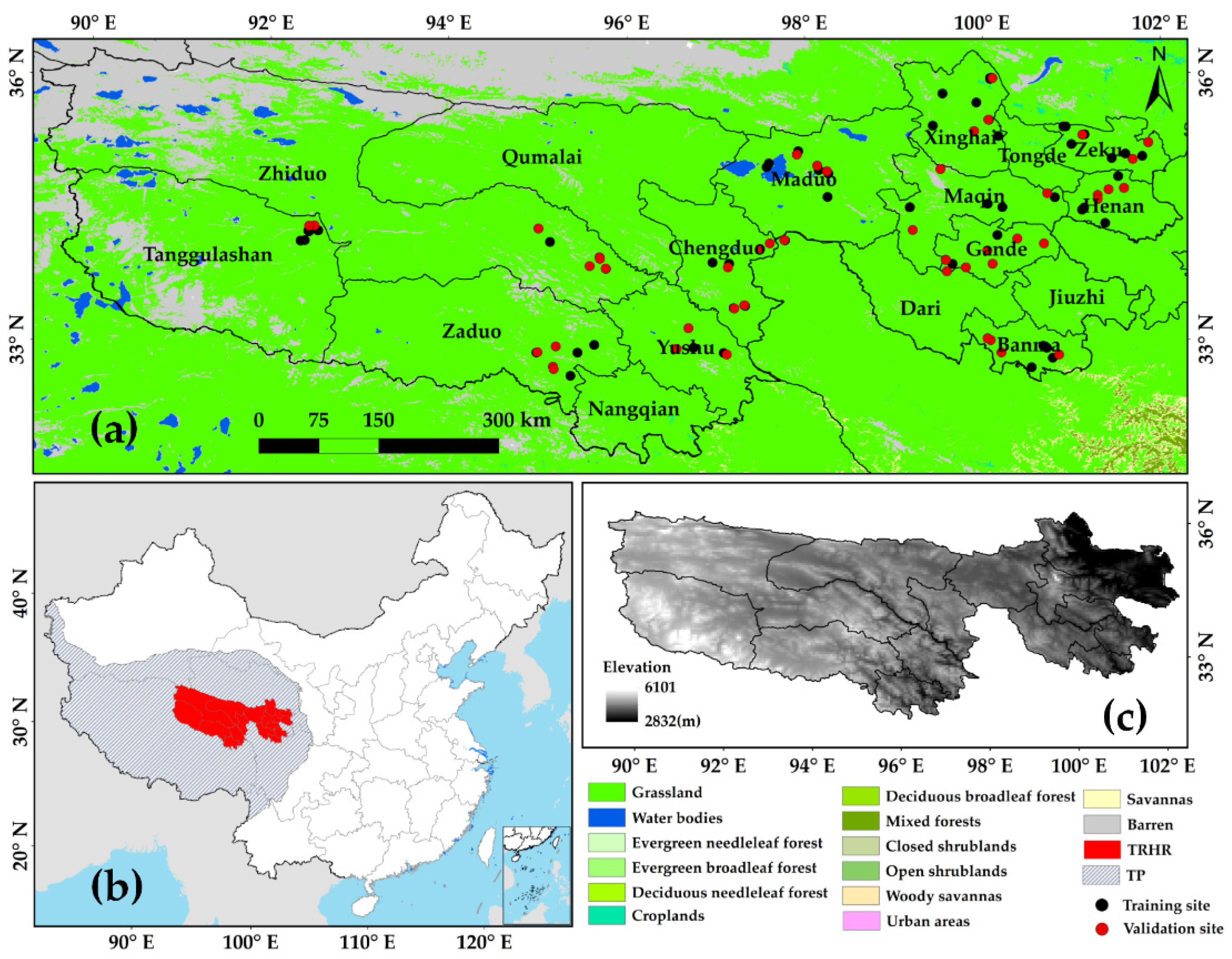
2.1. Study Area and In Situ Data
2.2. Remotely Sensed Data
2.3. Meteorological Data
2.4. Ancillary Data
3. Methodology
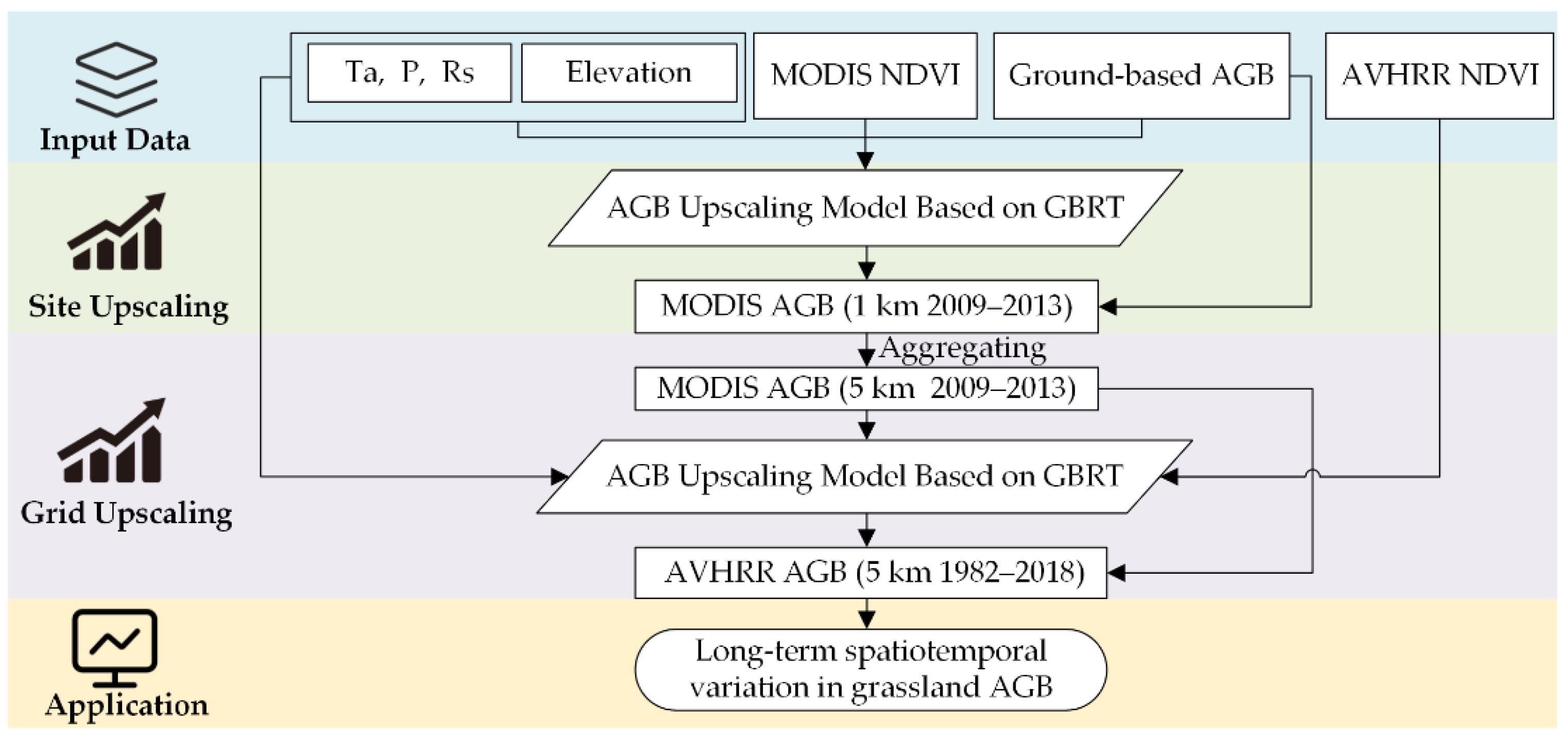
3.1. AGB Upscaled Procedure
3.2. GBRT
3.3. Other Machine Learning Methods
3.4. Statistical Metrics
4. Results
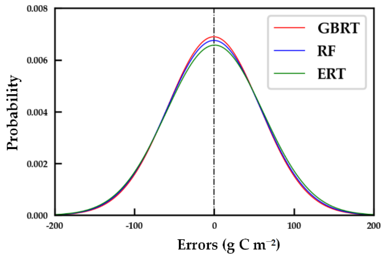
4.1. Evaluation of the AGB Upscaling Model from Ground Observations to a 1 KM Spatial Resolution
4.2. Evaluation of the AGB Upscaling Model at a 1 km to 5 km Spatial Resolution
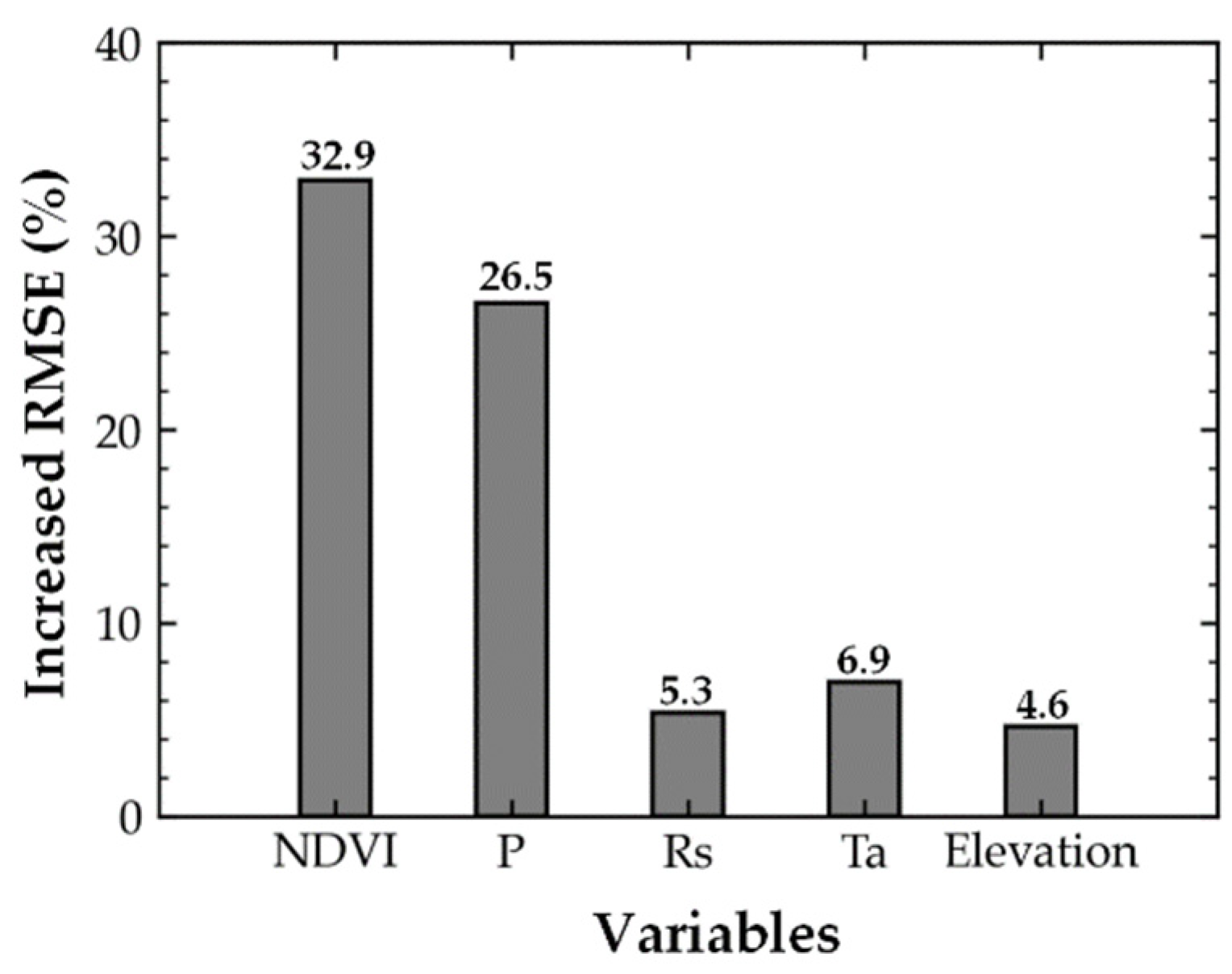
4.3. Importance of Input Variables to AGB Upscaling Model
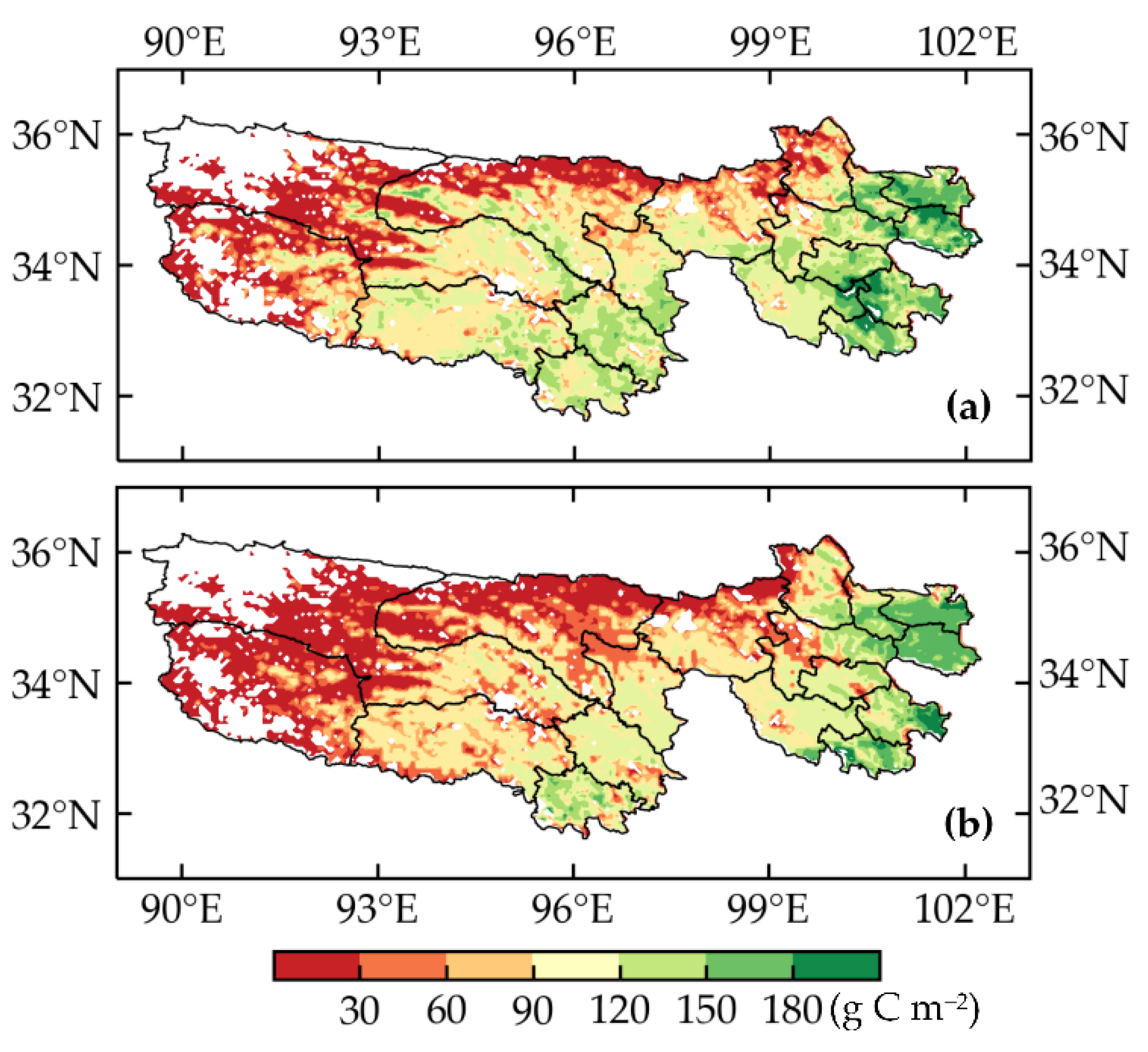
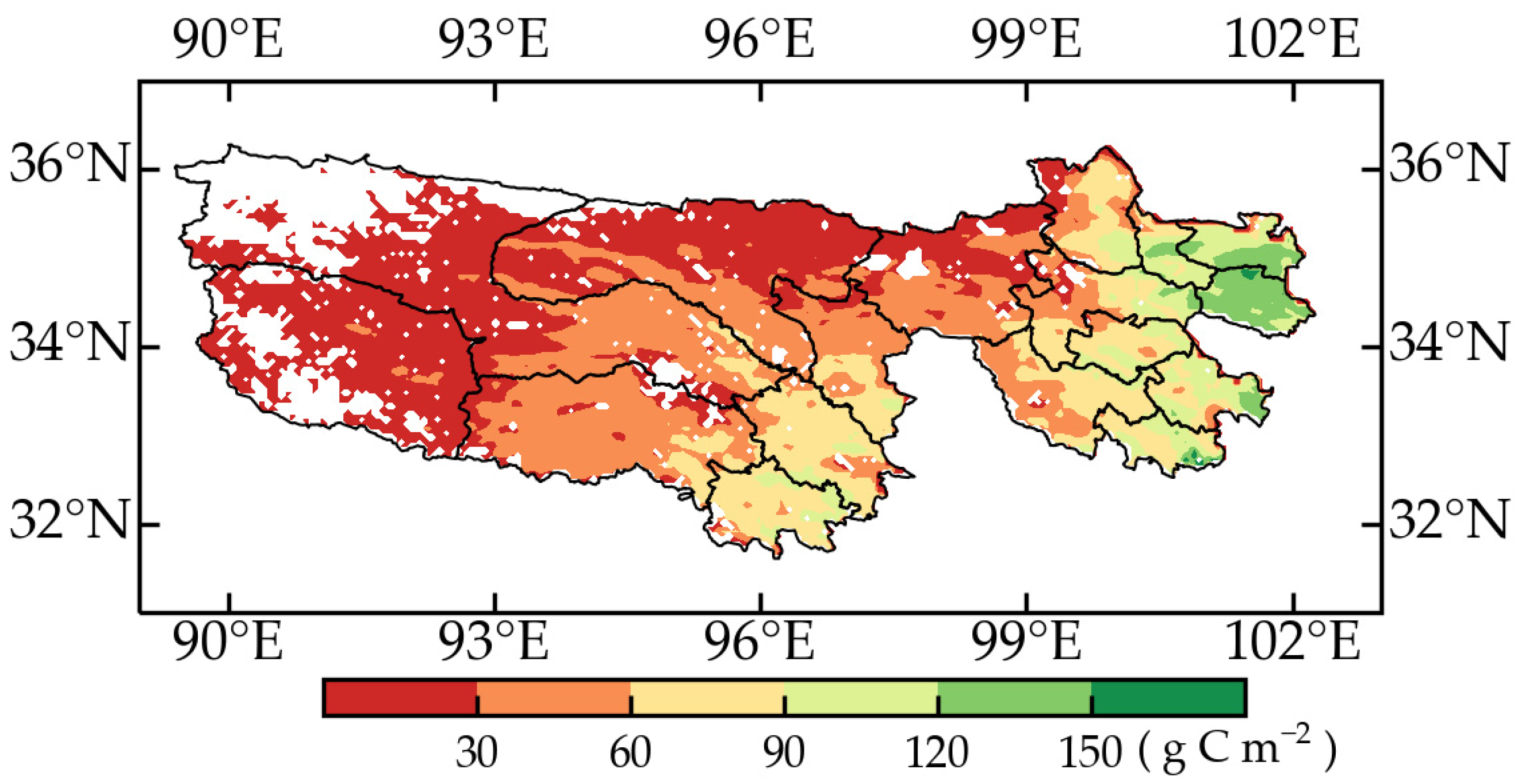
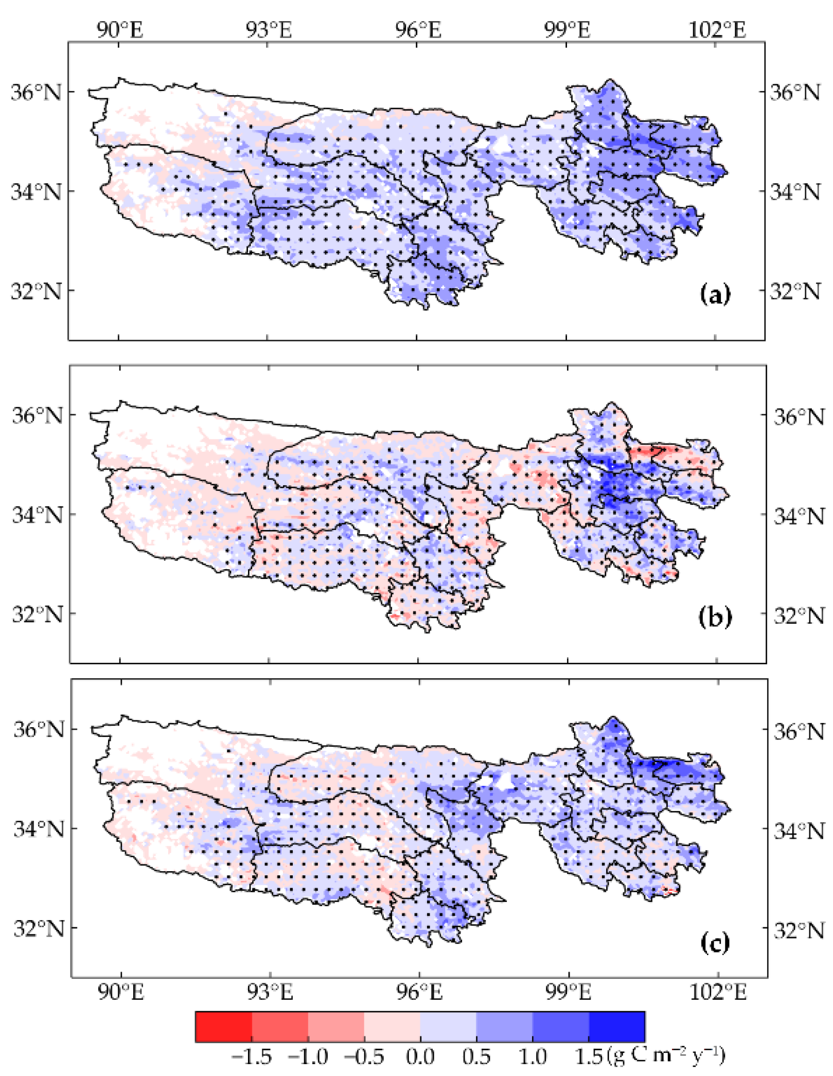
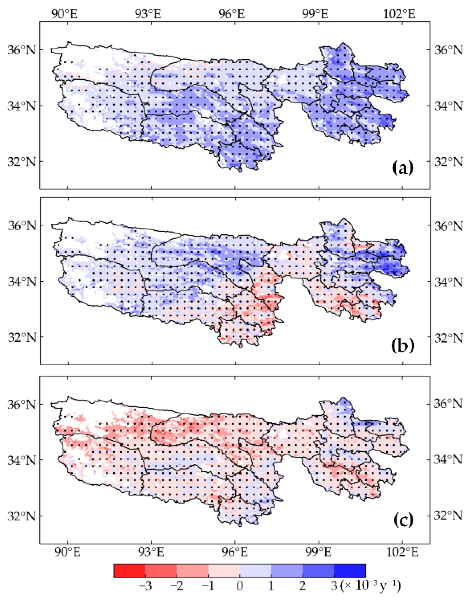
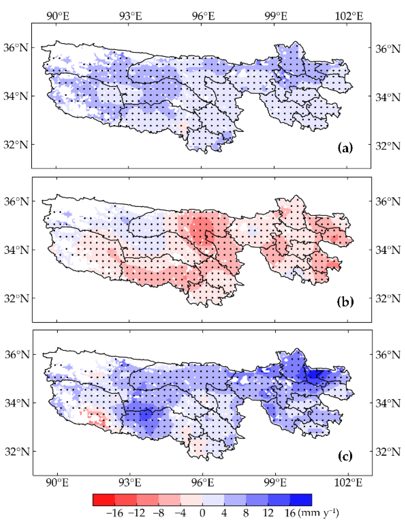
4.4. Spatiotemporal Variation in Grassland AGB during 1982–2018 in the TRHR
5. Discussion
5.1. Performance of AGB Upscaling Model
5.2. Spatiotemporal Variation in Grassland AGB during 1982–2018
5.3. Limitations and Outlooks for Future Study
6. Conclusions
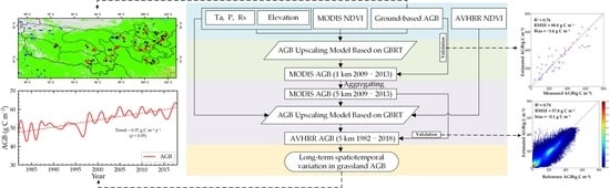
- (1)
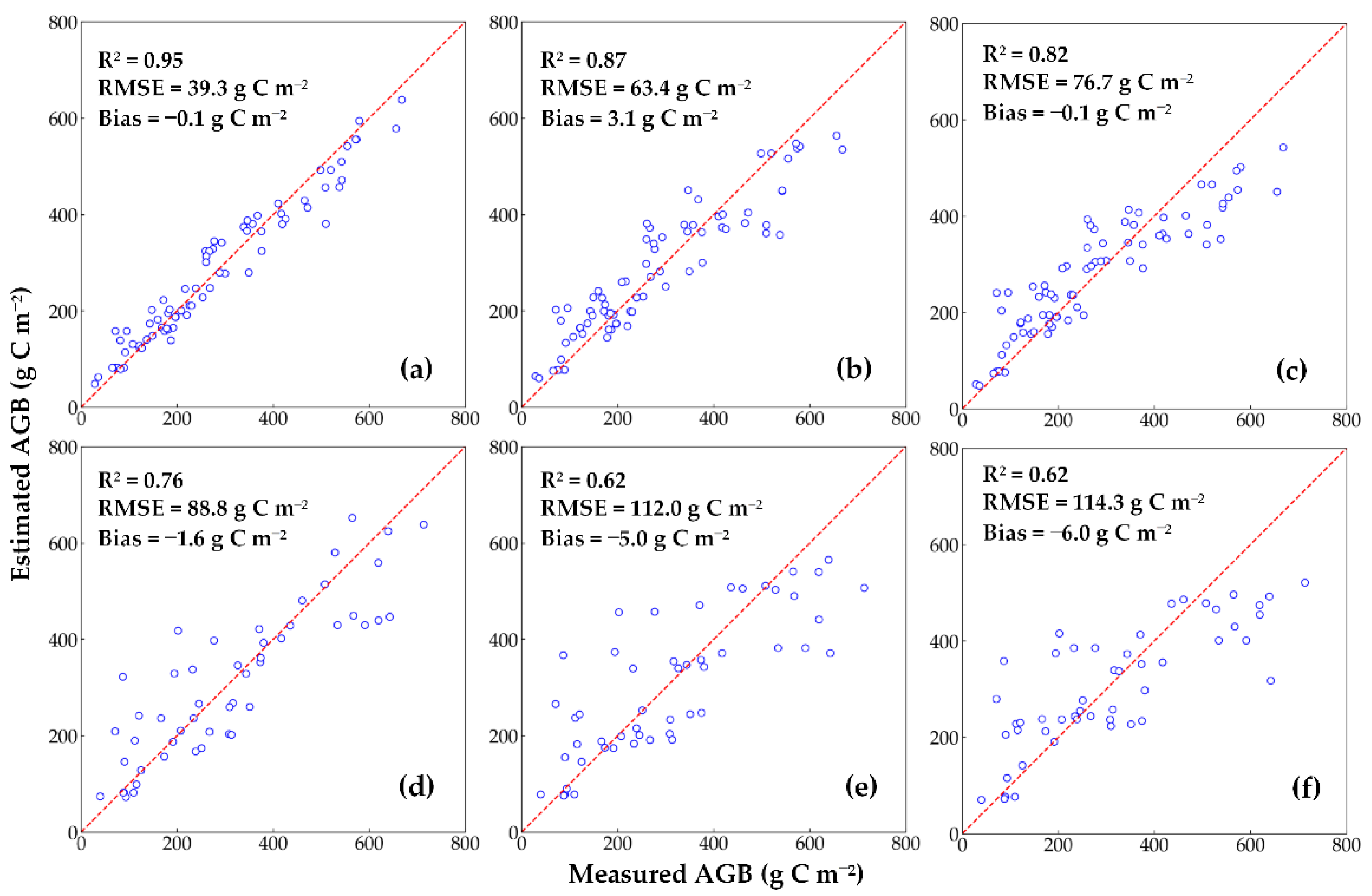
- MODIS-derived upscaled AGB with a 1 km spatial resolution based on the GBRT model was validated by AGB ground observations with the best performance (R2 = 0.76, RMSE = 88.8 g C m−2, and bias = −1.6 g C m−2).
- (2)
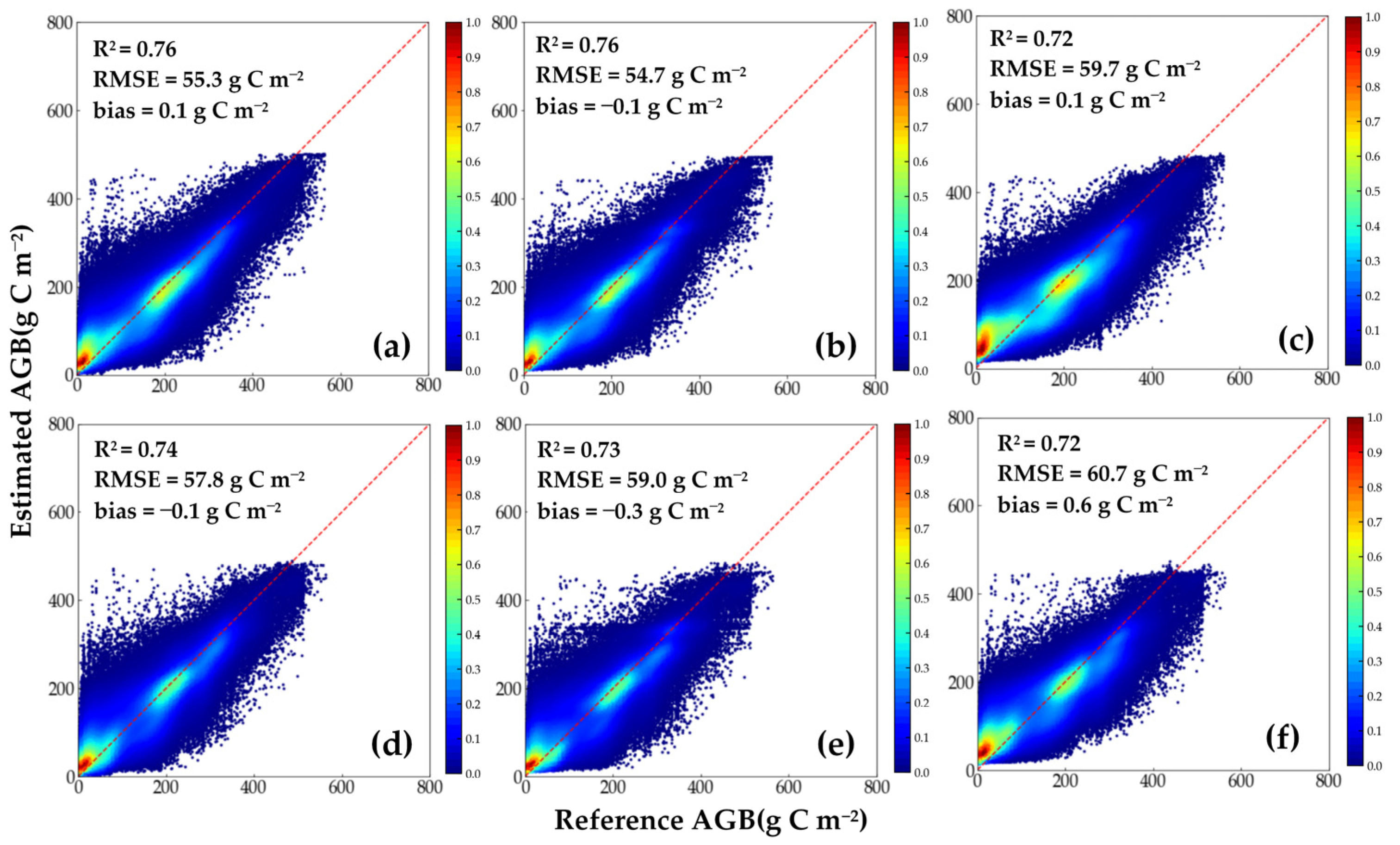
- The GBRT model also showed the best validation performance between the AVHRR-derived upscaled and MODIS-derived reference AGB with a 5 km spatial resolution with an R2 of 0.74, an RMSE of 57.8 g C m−2, and a bias of −0.1 g C m−2.
- (3)
- The annual trends of grassland AGB increased by 0.37 g C m−2 year−1 on average during 1982–2018, which was mainly attributed to vegetation greening and increasing precipitation.
Author Contributions
Funding
Institutional Review Board Statement
Informed Consent Statement
Data Availability Statement
Acknowledgments
Conflicts of Interest
References
- Scurlock, J.M.O.; Johnson, K.; Olson, R.J. Estimating net primary productivity from grassland biomass dynamics meas-urements. Glob. Chang. Biol. 2002, 8, 736–753. [Google Scholar] [CrossRef] [Green Version]
- Chopping, M.; Su, L.; Laliberte, A.; Rango, A.; Peters, D.P.; Kollikkathara, N. Mapping shrub abundance in desert grasslands using geometric-optical modeling and multi-angle remote sensing with CHRIS/Proba. Remote Sens. Environ. 2006, 104, 62–73. [Google Scholar] [CrossRef]
- Nie, X.-Q.; Yang, L.-C.; Xiong, F.; Li, C.-B.; Fan, L.; Zhou, G.-Y. Aboveground biomass of the alpine shrub ecosystems in Three-River Source Region of the Tibetan Plateau. J. Mt. Sci. 2018, 15, 357–363. [Google Scholar] [CrossRef]
- Gao, T.; Yang, X.; Jin, Y.; Ma, H.; Li, J.; Yu, H.; Yu, Q.; Zheng, X.; Xu, B. Spatio-Temporal Variation in Vegetation Biomass and Its Relationships with Climate Factors in the Xilingol Grasslands, Northern China. PLoS ONE 2013, 8, e83824. [Google Scholar] [CrossRef] [PubMed]
- Richardson, A.D.; Williams, M.; Hollinger, D.Y.; Moore, D.J.P.; Dail, D.B.; Davidson, E.A.; Scott, N.A.; Evans, R.S.; Hughes, H.; Lee, J.T.; et al. Estimating parameters of a forest ecosystem C model with measurements of stocks and fluxes as joint constraints. Oecologia 2010, 164, 25–40. [Google Scholar] [CrossRef] [PubMed]
- Xu, B.; Yang, X.C.; Tao, W.G.; Miao, J.M.; Yang, Z.; Liu, H.Q.; Jin, Y.X.; Zhu, X.H.; Qin, Z.H.; Lv, H.Y.; et al. MODIS-based remote-sensing monitoring of the spatiotemporal patterns of China’s grassland vegetation growth. Int. J. Remote Sens 2013, 34, 3867–3878. [Google Scholar] [CrossRef]
- Xu, D.; Guo, X. Some Insights on Grassland Health Assessment Based on Remote Sensing. Sensors 2015, 15, 3070–3089. [Google Scholar] [CrossRef] [Green Version]
- Tong, L.; Xu, X.; Fu, Y.; Li, S. Wetland Changes and Their Responses to Climate Change in the “Three-River Headwaters” Region of China since the 1990s. Energies 2014, 7, 2515–2534. [Google Scholar] [CrossRef] [Green Version]
- Heimann, M.; Reichstein, M. Terrestrial ecosystem carbon dynamics and climate feedbacks. Nat. Cell Biol. 2008, 451, 289–292. [Google Scholar] [CrossRef] [PubMed]
- Xia, J.; Ma, M.; Liang, T.; Wu, C.; Yang, Y.; Zhang, L.; Zhang, Y.; Yuan, W. Estimates of grassland biomass and turnover time on the Tibetan Plateau. Environ. Res. Lett. 2017, 13, 014020. [Google Scholar] [CrossRef]
- Klinge, H.; Rodrigues, W.A. Biomass estimation in a central amazonian rain-forest. Acta Cient. Venez. 1973, 24, 225–237. [Google Scholar]
- Steininger, M.K. Satellite estimation of tropical secondary forest above-ground biomass: Data from Brazil and Bolivia. Int. J. Remote Sens. 2000, 21, 1139–1157. [Google Scholar] [CrossRef]
- Dong, J.; Kaufmann, R.K.; Myneni, R.; Tucker, C.J.; Kauppi, P.E.; Liski, J.; Buermann, W.; Alexeyev, V.; Hughes, M.K. Remote sensing estimates of boreal and temperate forest woody biomass: Carbon pools, sources, and sinks. Remote Sens. Environ. 2003, 84, 393–410. [Google Scholar] [CrossRef] [Green Version]
- Segura, M.; Kanninen, M. Allometric Models for Tree Volume and Total Aboveground Biomass in a Tropical Humid Forest in Costa Rica. Biotropica 2005, 37, 2–8. [Google Scholar] [CrossRef]
- Xue, B.-L.; Guo, Q.; Hu, T.; Wang, G.; Wang, Y.; Tao, S.; Su, Y.; Liu, J.; Zhao, X. Evaluation of modeled global vegetation carbon dynamics: Analysis based on global carbon flux and above-ground biomass data. Ecol. Model. 2017, 355, 84–96. [Google Scholar] [CrossRef] [Green Version]
- Fan, J.; Zhong, H.; Harris, W.; Yu, G.; Wang, S.; Hu, Z.; Yue, Y. Carbon storage in the grasslands of China based on field measurements of above- and below-ground biomass. Clim. Chang. 2007, 86, 375–396. [Google Scholar] [CrossRef]
- Lim, K.; Treitz, P.; Wulder, M.; St-Onge, B.; Flood, M. LiDAR remote sensing of forest structure. Prog. Phys. Geogr. Earth Environ. 2003, 27, 88–106. [Google Scholar] [CrossRef] [Green Version]
- Lu, D. Aboveground biomass estimation using Landsat TM data in the Brazilian Amazon. Int. J. Remote Sens. 2005, 26, 2509–2525. [Google Scholar] [CrossRef]
- Santoro, M.; Beer, C.; Cartus, O.; Schmullius, C.; Shvidenko, A.; McCallum, I.; Wegmüller, U.; Wiesmann, A. Retrieval of growing stock volume in boreal forest using hyper-temporal series of Envisat ASAR ScanSAR backscatter measurements. Remote Sens. Environ. 2011, 115, 490–507. [Google Scholar] [CrossRef]
- Qi, W.; Dubayah, R.O. Combining Tandem-X InSAR and simulated GEDI lidar observations for forest structure mapping. Remote Sens. Environ. 2016, 187, 253–266. [Google Scholar] [CrossRef]
- Tucker, C.J. Red and photographic infrared linear combinations for monitoring vegetation. Remote Sens. Environ. 1979, 8, 127–150. [Google Scholar] [CrossRef] [Green Version]
- Tucker, C.J.; Justice, C.O.; Prince, S.D. Monitoring the grasslands of the Sahel 1984–1985. Int. J. Remote Sens. 1986, 7, 1571–1581. [Google Scholar] [CrossRef]
- Ullah, S.; Si, Y.; Schlerf, M.; Skidmore, A.; Shafique, M.; Iqbal, I.A. Estimation of grassland biomass and nitrogen using MERIS data. Int. J. Appl. Earth Obs. Geoinf. 2012, 19, 196–204. [Google Scholar] [CrossRef]
- Huete, A.; Justice, C.; Liu, H. Development of vegetation and soil indices for MODIS-EOS. Remote Sens. Environ. 1994, 49, 224–234. [Google Scholar] [CrossRef]
- Rondeaux, G.; Steven, M.; Baret, F. Optimization of soil-adjusted vegetation indices. Remote Sens. Environ. 1996, 55, 95–107. [Google Scholar] [CrossRef]
- Craine, J.M.; Nippert, J.; Elmore, A.; Skibbe, A.M.; Hutchinson, S.; Brunsell, N. Timing of climate variability and grassland productivity. Proc. Natl. Acad. Sci. USA 2012, 109, 3401–3405. [Google Scholar] [CrossRef] [Green Version]
- Li, F.; Zeng, Y.; Li, X.; Zhao, Q.; Wu, B. Remote sensing based monitoring of interannual variations in vegetation activity in China from 1982 to 2009. Sci. China Earth Sci. 2014, 57, 1800–1806. [Google Scholar] [CrossRef]
- Jia, W.; Liu, M.; Yang, Y.; He, H.; Zhu, X.; Yang, F.; Yin, C.; Xiang, W. Estimation and uncertainty analyses of grassland biomass in Northern China: Comparison of multiple remote sensing data sources and modeling approaches. Ecol. Indic. 2016, 60, 1031–1040. [Google Scholar] [CrossRef]
- Zhang, B.; Zhang, L.; Xie, D.; Yin, X.; Liu, C.; Liu, G. Application of Synthetic NDVI Time Series Blended from Landsat and MODIS Data for Grassland Biomass Estimation. Remote Sens. 2015, 8, 10. [Google Scholar] [CrossRef] [Green Version]
- Liang, T.; Yang, S.; Feng, Q.; Liu, B.; Zhang, R.; Huang, X.; Xie, H. Multi-factor modeling of above-ground biomass in alpine grassland: A case study in the Three-River Headwaters Region, China. Remote Sens. Environ. 2016, 186, 164–172. [Google Scholar] [CrossRef]
- Yang, S.; Feng, Q.; Liang, T.; Liu, B.; Zhang, W.; Xie, H. Modeling grassland above-ground biomass based on artificial neural network and remote sensing in the Three-River Headwaters Region. Remote Sens. Environ. 2018, 204, 448–455. [Google Scholar] [CrossRef]
- Zhou, W.; Li, H.; Xie, L.; Nie, X.; Wang, Z.; Du, Z.; Yue, T. Remote sensing inversion of grassland aboveground biomass based on high accuracy surface modeling. Ecol. Indic. 2021, 121, 107215. [Google Scholar] [CrossRef]
- Xu, B.; Yang, X.; Tao, W.; Qin, Z.; Liu, H.; Miao, J. Remote sensing monitoring upon the grass production in China. Acta Ecol. Sin. 2007, 27, 405–413. [Google Scholar] [CrossRef]
- Yang, Y.; Fang, J.; Pan, Y.; Ji, C. Aboveground biomass in Tibetan grasslands. J. Arid. Environ. 2009, 73, 91–95. [Google Scholar] [CrossRef]
- Fu, G.; Zhang, X.; Zhang, Y.; Shi, P.; Li, Y.; Zhou, Y.; Yang, P.; Shen, Z. Experimental warming does not enhance gross primary production and above-ground biomass in the alpine meadow of Tibet. J. Appl. Remote Sens. 2013, 7, 073505. [Google Scholar] [CrossRef] [Green Version]
- Jiang, Y.; Tao, J.; Huang, Y.; Zhu, J.; Tian, L.; Zhang, Y. The spatial pattern of grassland aboveground biomass on Xizang Plateau and its climatic controls. J. Plant Ecol. 2014, 8, 30–40. [Google Scholar] [CrossRef] [Green Version]
- Liu, S.; Cheng, F.; Dong, S.; Zhao, H.; Hou, X.; Wu, X. Spatiotemporal dynamics of grassland aboveground biomass on the Qinghai-Tibet Plateau based on validated MODIS NDVI. Sci. Rep. 2017, 7, 1–10. [Google Scholar] [CrossRef] [PubMed] [Green Version]
- Wu, J.; Fu, G. Modelling aboveground biomass using MODIS FPAR/LAI data in alpine grasslands of the Northern Tibetan Plateau. Remote Sens. Lett. 2018, 9, 150–159. [Google Scholar] [CrossRef]
- Cao, Y.; Wu, J.; Zhang, X.; Niu, B.; Li, M.; Zhang, Y.; Wang, X.; Wang, Z. Dynamic forage-livestock balance analysis in alpine grasslands on the Northern Tibetan Plateau. J. Environ. Manag. 2019, 238, 352–359. [Google Scholar] [CrossRef]
- Zeng, N.; Ren, X.; He, H.; Zhang, L.; Zhao, D.; Ge, R.; Li, P.; Niu, Z. Estimating grassland aboveground biomass on the Tibetan Plateau using a random forest algorithm. Ecol. Indic. 2019, 102, 479–487. [Google Scholar] [CrossRef]
- Gao, X.; Dong, S.; Li, S.; Xu, Y.; Liu, S.; Zhao, H.; Yeomans, J.; Li, Y.; Shen, H.; Wu, S.; et al. Using the random forest model and validated MODIS with the field spectrometer measurement promote the accuracy of estimating aboveground biomass and coverage of alpine grasslands on the Qinghai-Tibetan Plateau. Ecol. Indic. 2020, 112, 106114. [Google Scholar] [CrossRef]
- Chu, D. Aboveground biomass estimates of grassland in the North Tibet using modis remote sensing approaches. Appl. Ecol. Environ. Res. 2020, 18, 7655–7672. [Google Scholar] [CrossRef]
- Yu, L.; Zhou, L.; Liu, W.; Zhou, H.-K. Using Remote Sensing and GIS Technologies to Estimate Grass Yield and Livestock Carrying Capacity of Alpine Grasslands in Golog Prefecture, China. Pedosphere 2010, 20, 342–351. [Google Scholar] [CrossRef]
- Ma, Q.; Chai, L.; Hou, F.; Chang, S.; Ma, Y.; Tsunekawa, A.; Cheng, Y. Quantifying Grazing Intensity Using Remote Sensing in Alpine Meadows on Qinghai-Tibetan Plateau. Sustainability 2019, 11, 417. [Google Scholar] [CrossRef] [Green Version]
- Kong, B.; Yu, H.; Du, R.; Wang, Q. Quantitative Estimation of Biomass of Alpine Grasslands Using Hyperspectral Remote Sensing. Rangel. Ecol. Manag. 2019, 72, 336–346. [Google Scholar] [CrossRef]
- An, R.; Wang, H.-L.; Feng, X.-Z.; Wu, H.; Wang, Z.; Wang, Y.; Shen, X.-J.; Lu, C.-H.; Quaye-Ballard, J.A.; Chen, Y.-H.; et al. Monitoring rangeland degradation using a novel local NPP scaling based scheme over the “Three-River Headwaters” region, hinterland of the Qinghai-Tibetan Plateau. Quat. Int. 2017, 444, 97–114. [Google Scholar] [CrossRef] [Green Version]
- Xiao, Z.; Liang, S.; Tian, X.; Jia, K.; Yao, Y.; Jiang, B. Reconstruction of Long-Term Temporally Continuous NDVI and Surface Reflectance From AVHRR Data. IEEE J. Sel. Top. Appl. Earth Obs. Remote Sens. 2017, 10, 5551–5568. [Google Scholar] [CrossRef]
- Xiao, Z.Q.; Liang, S.L.; Wang, T.T.; Liu, Q. Reconstruction of satellite-retrieved land-surface reflectance based on tempo-rally-continuous vegetation indices. Remote Sens. 2015, 7, 9844–9864. [Google Scholar] [CrossRef] [Green Version]
- Beer, C.; Reichstein, M.; Tomelleri, E.; Ciais, P.; Jung, M.; Carvalhais, N.; Rödenbeck, C.; Arain, M.A.; Baldocchi, D.; Bonan, G.B.; et al. Terrestrial gross carbon dioxide uptake: Global distribution and covariation with climate. Science 2010, 329, 834–838. [Google Scholar] [CrossRef] [Green Version]
- Anav, A.; Friedlingstein, P.; Beer, C.; Ciais, P.; Harper, A.; Jones, C.D.W.; Murray-Tortarolo, G.; Papale, D.; Parazoo, N.C.; Peylin, P.; et al. Spatiotemporal patterns of terrestrial gross primary production: A review. Rev. Geophys. 2015, 53, 785–818. [Google Scholar] [CrossRef] [Green Version]
- Jung, M.; Reichstein, M.; Bondeau, A. Towards global empirical upscaling of FLUXNET eddy covariance observations: Vali-dation of a model tree ensemble approach using a biosphere model. Biogeosciences 2009, 6, 2001–2013. [Google Scholar] [CrossRef] [Green Version]
- Jung, M.; Reichstein, M.; Margolis, H.A.; Cescatti, A.; Richardson, A.D.; Arain, M.A.; Arneth, A.; Bernhofer, C.; Bonal, D.; Chen, J.; et al. Global patterns of land-atmosphere fluxes of carbon dioxide, latent heat, and sensible heat derived from eddy covariance, satellite, and meteorological observations. J. Geophys. Res. Biogeosci. 2011, 116. [Google Scholar] [CrossRef] [Green Version]
- Yuan, X.; Li, L.; Tian, X.; Luo, G.; Chen, X. Estimation of above-ground biomass using MODIS satellite imagery of multiple land-cover types in China. Remote Sens. Lett. 2016, 7, 1141–1149. [Google Scholar] [CrossRef]
- Fang, Y. Managing the Three-Rivers Headwater Region, China: From Ecological Engineering to Social Engineering. Ambio 2013, 42, 566–576. [Google Scholar] [CrossRef] [Green Version]
- Feng, Y.; Wu, J.; Zhang, J.; Zhang, X.; Song, C. Identifying the Relative Contributions of Climate and Grazing to Both Direction and Magnitude of Alpine Grassland Productivity Dynamics from 1993 to 2011 on the Northern Tibetan Plateau. Remote Sens. 2017, 9, 136. [Google Scholar] [CrossRef] [Green Version]
- Huete, A.; Didan, K.; Miura, T.; Rodriguez, E.P.; Gao, X.; Ferreira, L.G. Overview of the radiometric and biophysical per-formance of the MODIS vegetation indices. Remote Sens. Environ. 2002, 83, 195–213. [Google Scholar] [CrossRef]
- Yang, K.; He, J. China meteorological forcing dataset (1979–2018). Big Earth Data Platf. Three Poles 2019. [Google Scholar] [CrossRef]
- Chen, Y.; Yang, K.; He, J.; Qin, J.; Shi, J.; Du, J.; He, Q. Improving land surface temperature modeling for dry land of China. J. Geophys. Res. Space Phys. 2011, 116, 15. [Google Scholar] [CrossRef]
- Huffman, G.J.; Bolvin, D.T.; Nelkin, E.J.; Wolff, D.B.; Adler, R.F.; Gu, G.; Hong, Y.; Bowman, K.P.; Stocker, E.F. The TRMM Multisatellite Precipitation Analysis (TMPA): Quasi-Global, Multiyear, Combined-Sensor Precipitation Estimates at Fine Scales. J. Hydrometeorol. 2007, 8, 38–55. [Google Scholar] [CrossRef]
- Yatagai, A.; Arakawa, O.; Kamiguchi, K.; Kawamoto, H.; Nodzu, M.I.; Hamada, A. A 44-Year Daily Gridded Precipitation Dataset for Asia Based on a Dense Network of Rain Gauges. Sola 2009, 5, 137–140. [Google Scholar] [CrossRef] [Green Version]
- Yang, K.; He, J.; Tang, W.; Qin, J.; Cheng, C.C. On downward shortwave and longwave radiations over high altitude regions: Observation and modeling in the Tibetan Plateau. Agric. For. Meteorol. 2010, 150, 38–46. [Google Scholar] [CrossRef]
- Yao, Y.; Liang, S.; Li, X.; Chen, J.; Wang, K.; Jia, K.; Cheng, J.; Jiang, B.; Fisher, J.B.; Mu, Q.; et al. A satellite-based hybrid algorithm to determine the Priestley–Taylor parameter for global terrestrial latent heat flux estimation across multiple biomes. Remote Sens. Environ. 2015, 165, 216–233. [Google Scholar] [CrossRef] [Green Version]
- Hansen, M.C.; DeFries, R.S.; Townshend, J.R.G.; Sohlberg, R.A. Global land cover classification at 1 km spatial resolution using a classification tree approach. Int. J. Remote Sens. 2000, 21, 1331–1364. [Google Scholar] [CrossRef]
- Friedman, J.H. Greedy function approximation: A gradient boosting machine. Ann. Stat. 2001, 29, 1189–1232. [Google Scholar] [CrossRef]
- Yang, L.; Liang, S.; Zhang, Y. A New Method for Generating a Global Forest Aboveground Biomass Map From Multiple High-Level Satellite Products and Ancillary Information. IEEE J. Sel. Top. Appl. Earth Obs. Remote Sens. 2020, 13, 2587–2597. [Google Scholar] [CrossRef]
- Breiman, L. Random forests. Mach. Learn. 2001, 45, 5–32. [Google Scholar] [CrossRef] [Green Version]
- Breiman, L. Bagging predictors. Mach. Learn. 1996, 24, 123–140. [Google Scholar] [CrossRef] [Green Version]
- Chatterjee, A.; Lahiri, S.N. Bootstrapping Lasso Estimators. J. Am. Stat. Assoc. 2011, 106, 608–625. [Google Scholar] [CrossRef]
- Abowarda, A.S.; Bai, L.; Zhang, C.; Long, D.; Li, X.; Huang, Q.; Sun, Z. Generating surface soil moisture at 30 m spatial resolution using both data fusion and machine learning toward better water resources management at the field scale. Remote Sens. Environ. 2021, 255, 112301. [Google Scholar] [CrossRef]
- Xu, T.R.; Guo, Z.X.; Liu, S.M.; He, X.L.; Meng, Y.F.Y.; Xu, Z.W.; Xia, Y.L.; Xiao, J.F.; Zhang, Y.; Ma, Y.F.; et al. Evaluating diffferent machine learning methods for upscaling evapotranspiration from flux towers to the regional scale. J. Geophys. Res. Atmos. 2018, 123, 8674–8690. [Google Scholar] [CrossRef]
- Geurts, P.; Ernst, D.; Wehenkel, L. Extremely randomized trees. Mach. Learn. 2006, 63, 3–42. [Google Scholar] [CrossRef] [Green Version]
- Shang, K.; Yao, Y.; Li, Y.; Yang, J.; Jia, K.; Zhang, X.; Chen, X.; Bei, X.; Guo, X. Fusion of Five Satellite-Derived Products Using Extremely Randomized Trees to Estimate Terrestrial Latent Heat Flux over Europe. Remote Sens. 2020, 12, 687. [Google Scholar] [CrossRef] [Green Version]
- Sneyres, R. Technical Note no. 143 on the Statistical Analysis of Time Series of Observation; World Meteorological Organization: Geneva, Switzerland, 1990. [Google Scholar]
- Nasri, M.; Modarres, R. Dry spell trend analysis of Isfahan Province, Iran. Int. J. Clim. 2009, 29, 1430–1438. [Google Scholar] [CrossRef]
- Song, L.; Zhuang, Q.; Yin, Y.; Zhu, X.; Wu, S. Spatio-temporal dynamics of evapotranspiration on the Tibetan Plateau from 2000 to 2010. Environ. Res. Lett. 2017, 12, 014011. [Google Scholar] [CrossRef]
- Zhu, S.; Xiao, Z.; Luo, X.; Zhang, H.; Liu, X.; Wang, R.; Zhang, M.; Huo, Z. Multidimensional Response Evaluation of Remote-Sensing Vegetation Change to Drought Stress in the Three-River Headwaters, China. IEEE J. Sel. Top. Appl. Earth Obs. Remote Sens. 2020, 13, 6249–6259. [Google Scholar] [CrossRef]
- Lauenroth, W.K.; Sala, O.E. Long-Term Forage Production of North American Shortgrass Steppe. Ecol. Appl. 1992, 2, 397–403. [Google Scholar] [CrossRef] [PubMed] [Green Version]
- Bai, Y.; Liang, S.; Yuan, W. Estimating Global Gross Primary Production from Sun-Induced Chlorophyll Fluorescence Data and Auxiliary Information Using Machine Learning Methods. Remote Sens. 2021, 13, 963. [Google Scholar] [CrossRef]
- Yang, L.; Zhang, X.; Liang, S.; Yao, Y.; Jia, K.; Jia, A. Estimating Surface Downward Shortwave Radiation over China Based on the Gradient Boosting Decision Tree Method. Remote Sens. 2018, 10, 185. [Google Scholar] [CrossRef] [Green Version]
- Jia, K.; Yang, L.; Liang, S.; Xiao, Z.; Zhao, X.; Yao, Y.; Zhang, X.; Jiang, B.; Liu, D. Long-Term Global Land Surface Satellite (GLASS) Fractional Vegetation Cover Product Derived From MODIS and AVHRR Data. IEEE J. Sel. Top. Appl. Earth Obs. Remote Sens. 2018, 12, 508–518. [Google Scholar] [CrossRef]
- Lehnert, L.; Meyer, H.; Wang, Y.; Miehe, G.; Thies, B.; Reudenbach, C.; Bendix, J. Retrieval of grassland plant coverage on the Tibetan Plateau based on a multi-scale, multi-sensor and multi-method approach. Remote Sens. Environ. 2015, 164, 197–207. [Google Scholar] [CrossRef]
- Bei, X.Y.; Yao, Y.J.; Zhang, L.L.; Xu, T.R.; Jia, K.; Zhang, X.T.; Shang, K.; Xu, J.; Chen, X.W. Long-Term spatiotemporal dynamics of terrestrial biophysical variables in the Three-River Headwaters Region of China from satellite and meteoro-logical datasets. Remote Sens. 2019, 11, 25. [Google Scholar] [CrossRef] [Green Version]
- Peng, J.; Liu, Z.; Liu, Y.; Wu, J.; Han, Y. Trend analysis of vegetation dynamics in Qinghai–Tibet plateau using hurst exponent. Ecol. Indic. 2012, 14, 28–39. [Google Scholar] [CrossRef]
- Xu, M.; Kang, S.; Chen, X.; Wu, H.; Wang, X.; Su, Z. Detection of hydrological variations and their impacts on vegetation from multiple satellite observations in the Three-River Source Region of the Tibetan Plateau. Sci. Total. Environ. 2018, 639, 1220–1232. [Google Scholar] [CrossRef] [PubMed]
- Chen, Y.; Xia, J.; Liang, S.; Feng, J.; Fisher, J.; Li, X.; Li, X.; Liu, S.; Ma, Z.; Miyata, A.; et al. Comparison of satellite-based evapotranspiration models over terrestrial ecosystems in China. Remote Sens. Environ. 2014, 140, 279–293. [Google Scholar] [CrossRef]
- Friend, A.D.; Arneth, A.; Kiang, N.Y.; Lomas, M.; Ogee, J.; Rödenbeck, C.; Running, S.W.; Santaren, J.-D.; Sitch, S.; Viovy, N.; et al. FLUXNET and modelling the global carbon cycle. Glob. Chang. Biol. 2007, 13, 610–633. [Google Scholar] [CrossRef]
- Yuan, W.; Liu, S.; Yu, G.; Bonnefond, J.-M.; Chen, J.; Davis, K.; Desai, A.R.; Goldstein, A.; Gianelle, D.; Rossi, F.; et al. Global estimates of evapotranspiration and gross primary production based on MODIS and global meteorology data. Remote Sens. Environ. 2010, 114, 1416–1431. [Google Scholar] [CrossRef] [Green Version]


| Study Domain | Time Horizon | Remotely Sensed Data | Models | Main Conclusions | References |
|---|---|---|---|---|---|
| TP | 2005 | MODIS NDVI product | Exponential model | Estimated precision of AGB in the TP is 80%. | [33] |
| TP | 2001–2004 | MODIS EVI product | EVI-based linear model | Approximately 54.2% of AGB variation in alpine grasslands could be explained by climatic variables and soil texture. | [34] |
| Golog Prefecture | 2005.7–9 | MODIS NDVI and EVI products | Exponential model | NDVI-based exponential model is optimal, and the precision was approximately 72%. | [43] |
| TP | 2000–2012 | MODIS NDVI product | Exponential model | The accuracy of model (AGB = 10.33e3.28NDVI) is R2 = 0.64. | [35] |
| TP | 2011–2012 | MODIS NDVI, EVI and reflectance products | General linear model | Large spatial variation of AGB in the TP was observed and AGB ranged from 1 to 136 g/m2. | [36] |
| TRHR | 2003–2014 | MODIS reflectance product | Multi-factors regression model | Multifactor model based on latitude, longitude, and grass cover is selected as the AGB model (R2 = 0.63). | [30] |
| TP | 2000–2012 | MODIS NDVI product | Linear and power models | For meadow grasslands, linear model is the best AGB estimation model (R2 = 0.51, RMSE = 139.5 kg/hm2). For steppe grasslands, power function is the best AGB estimation model (R2 = 0.63, RMSE = 146.5 kg/hm2). | [37] |
| NTP | 2000–2013 | MODIS FPAR/LAI product | Logarithm model | Aqua MODIS FPAR/LAI product may have the highest accuracy in AGB estimation. | [38] |
| TRHR | 2001–2016 | MODIS surface reflectance product | ANN model | ANN model based on grass cover, longitude, latitude, and NDVI has best accuracy (R2 = 0.62, RMSE = 589.9 kg/DW ha) in testing set. | [31] |
| Maqu | 2016–2017 | MODIS NDVI and EVI products | Linear model | R2 of the NDVI models were all greater than those of the EVI models. | [44] |
| NTP | 2000–2014 | MODIS NDVI product | logarithm and exponent models | The slopes of AGB in fenced grasslands and in livestock were −2.71 and −0.15 g m−2 year−1, respectively. | [39] |
| Shenzha | 2000–2013 | MODIS NDVI product | Exponential model | Annual average AGB was slightly increased and fluctuated between 1800 and 2700 kg/ha, with an average of 2272 kg/ha. | [45] |
| TP | 2000–2014 | MODIS NDVI and EVI products | RF model | Grassland AGB decreased from southeast to northwest with an average value of 77.12 g m−2 and increasing rate of 0.19 g m−2 year−1 in the TP. | [40] |
| TP | 2000–2017 | MODIS NDVI product | RF model | RF model with multiple factors performed best for AGB estimation (R2 = 0.75, RMSE = 346.06 kg/ha). | [41] |
| NTP | 2004.9 | MODIS NDVI and EVI products | NDVI-based exponential model | Optimal regression model for AGB estimation was NDVI-based exponential models (R2 = 0.63). | [42] |
| TRHR | 2001–2019 | MODIS NDVI product | HASM | HASM achieved the best results (R2 = 0.85, RMSE = 29 g m−2) and AGB increased by 1 g m−2 year−1. | [32] |
Publisher’s Note: MDPI stays neutral with regard to jurisdictional claims in published maps and institutional affiliations. |
© 2021 by the authors. Licensee MDPI, Basel, Switzerland. This article is an open access article distributed under the terms and conditions of the Creative Commons Attribution (CC BY) license (https://creativecommons.org/licenses/by/4.0/).
Share and Cite
Yu, R.; Yao, Y.; Wang, Q.; Wan, H.; Xie, Z.; Tang, W.; Zhang, Z.; Yang, J.; Shang, K.; Guo, X.; et al. Satellite-Derived Estimation of Grassland Aboveground Biomass in the Three-River Headwaters Region of China during 1982–2018. Remote Sens. 2021, 13, 2993. https://0-doi-org.brum.beds.ac.uk/10.3390/rs13152993
Yu R, Yao Y, Wang Q, Wan H, Xie Z, Tang W, Zhang Z, Yang J, Shang K, Guo X, et al. Satellite-Derived Estimation of Grassland Aboveground Biomass in the Three-River Headwaters Region of China during 1982–2018. Remote Sensing. 2021; 13(15):2993. https://0-doi-org.brum.beds.ac.uk/10.3390/rs13152993
Chicago/Turabian StyleYu, Ruiyang, Yunjun Yao, Qiao Wang, Huawei Wan, Zijing Xie, Wenjia Tang, Ziping Zhang, Junming Yang, Ke Shang, Xiaozheng Guo, and et al. 2021. "Satellite-Derived Estimation of Grassland Aboveground Biomass in the Three-River Headwaters Region of China during 1982–2018" Remote Sensing 13, no. 15: 2993. https://0-doi-org.brum.beds.ac.uk/10.3390/rs13152993