
Moving Target Shadow Analysis and Detection for ViSAR Imagery


1
College of Electronic Science and Engineering, National University of Defense Technology (NUDT), Changsha 410073, China
2
Beijing Institute of Remote Sensing Information, Beijing 100192, China
*
Author to whom correspondence should be addressed.
Remote Sens. 2021, 13(15), 3012; https://0-doi-org.brum.beds.ac.uk/10.3390/rs13153012
Submission received: 26 June 2021
/
Revised: 19 July 2021
/
Accepted: 28 July 2021
/
Published: 31 July 2021
(This article belongs to the Topic High-Resolution Earth Observation Systems, Technologies, and Applications)
Abstract
:The video synthetic aperture radar (ViSAR) is a new application in radar techniques. ViSAR provides high- or moderate-resolution SAR images with a faster frame rate, which permits the detection of the dynamic changes in the interested area. A moving target with moderate velocity can be detected by shadow detection in ViSAR. This paper analyses the frame rate and the shadow feature, discusses the velocity limitation of ViSAR moving target shadow detection and quantitatively gives the expression of velocity limitation. Furthermore, a fast factorized back projection (FFBP) based SAR video formation method and a shadow-based ground moving target detection method are proposed to generate SAR videos and detect the moving target shadow. The experimental results with simulated data prove the validity and feasibility of the proposed quantitative analysis and the proposed methods.

1. Introduction
Synthetic aperture radar (SAR) is a remote-sensing sensor with a high resolution, which can work well day-and-night and weather-independently. Its high-resolution image productions are applied in remote sensing applications, e.g., earth observation, marine surveillance, earthquake and volcano detection, interferometry, and differential interferometry [1,2,3,4,5,6,7]. Video SAR (ViSAR) is a new technique which acquires a sequence of radar images and displays them with a video stream [8,9,10]. This technique combines the advantages of SAR high resolution and video dynamic display to achieve a continuous-and-high-resolution dynamic surveillance of the interested area. Moreover, its frame rates and video streams allow for a temporal context that is suitable for a natural interpretation by human eyes.
Moving target recognition is an important application in SAR signal processing. The Doppler shift will emerge when a moving target owns a velocity component along the direction of radar Line-of-Sight (LOS), which is represented as a displacement of the target energy return. With the loss of illumination from a radar wave, the actual location of the moving target will show an obvious shadow feature. Compared with the conventional SAR ground moving target indicator (GMTI) based method, the shadow-based method for ViSAR moving target detection has the advantages of a high positioning accuracy, high detection rate and low minimum detectable speed. Hence, it can be utilized as a promising technique for moving target detection (MTD) in ViSAR, especially for reconnaissance and surveillance of slow speed moving targets on the ground.
In an SAR image, both targets with a low radar cross section (RCS) and scene regions with short radar illumination present like shadows. This mechanism makes moving targets with a moderate velocity visible in the ViSAR image frames. The energy distribution of a moving target in a ViSAR image is blurred and displaced while the shadow of moving target lies on its true location. Shadow detection for a moving target can be a supplementary method in moving target indication. Hence, the radar video offers practical understanding of the target motion without added implementation such as usual moving target indication [11]. In recent years, shadow detection has become a hot topic in ViSAR application. Ref. [12] enhanced the moving target shadow in ViSAR images by adopting the method of fixed focus shadow enhancement (FFSE), ref. [13] achieved moving target detection in SAR imagery by tracking the moving target shadow over adjacent continuous looks. Based on shadow intensity and phase features, ref. [14] presents a method of detecting moving targets. However, the velocity limitation of a moving target is not discussed in the shadow formation [12,13,14,15,16,17,18,19,20,21,22]. Based on compressed sensing (CS), ref. [20] presents a method to estimate the velocity of a moving target. However, the results of this method are mean velocities of moving targets. This method cannot indicate the real positions of moving targets, which limits the applications of moving target real-time tracking.
In this paper, firstly the mechanism of the moving target shadow is preliminarily analyzed and then the velocity detected limitation which is based on the moving target shadow is given. The analysis presented in this paper can be referenced as the foundation for radar system design or predetermination of moving target detection based on shadows.
The main contributions of this paper can be summarized as follows:
- (1)
- A fast factorized back projection (FFBP) based SAR video frame formation method: This processing method generates high matching SAR video directly from SAR echo, which has the advantages of being applicable to multi-mode SAR data, no additional registration processing, flexible use, high accuracy and high computational efficiency.
- (2)
- Shadow formation mechanism and velocity condition analysis: Based on SAR imaging mechanism and the radar equation, the relationship between shadow and scattering characteristics, illumination time, imaging geometry, target size, processing parameters, etc. is analyzed, and the velocity condition of ground shadow formation under given parameters is obtained, which provides the basis for ViSAR system design and shadow-based moving target detection processing.
- (3)
- ViSAR shadow detection method: Based on the analysis of the shadow features of ViSAR, a shadow detection method of moving target is adopted, which combines background difference and symmetric difference. The basic idea is to make full use of the time information of a ViSAR sequential image and the shadow features. It has the advantages of fast calculation and good robustness.
The paper is organized as follows. In Section 2, the ViSAR frame rate is discussed and the SAR video formation method is introduced. In Section 3, the mechanism of shadow is analyzed and the velocity detected limitation is deduced. After that, a shadow-based ground moving target detection method is proposed. The uniform scene simulation and real data simulation are given in Section 4 to prove the views presented in this paper. Finally, conclusions are drawn in Section 5.
2. ViSAR Formation
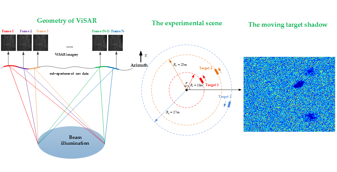
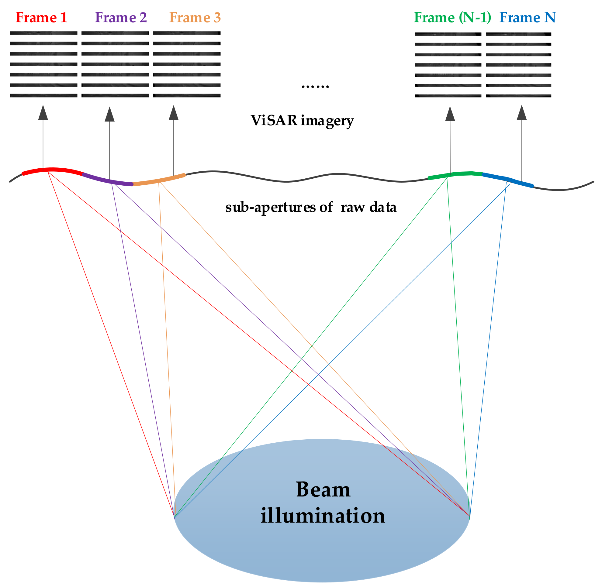
ViSAR is a land-imaging mode whereby the SAR system is operated in a sliding spotlight/spotlight or a circular configuration for an extended period of time. ViSAR illuminates the interested area by steering its antenna (sliding spotlight/spotlight mode) or changing its trajectories (circular mode) during the mission and it formats the frames using sub-aperture data. Figure 1 shows the geometry of spotlight mode ViSAR. The ViSAR system provides the continuous acquisition and processing of phase history domain data. By continuously imaging the sub-aperture data, continuous frames are obtained [12,23]. The video generation can be in real time or after the collection of whole apertures. Whatever generating method, it should divide the raw data into sub-apertures according to the frame rate. Whether frames overlapped or not depends on the frame rate and carrier frequency of the radar system.
2.1. Frame Rate Analysis for ViSAR
The frame rate of ViSAR is a measurement of SAR video display frames, in units of frames per second (fps) or hertz (Hz). The frame rate perceivable by the general human eyes is 16–20 Hz, and the standard frame rate of a movie is 24 Hz. The frame rate of a typical optical video satellite can reach up to 30 Hz.
Unlike optical instantaneous imaging, ViSAR requires a certain cumulative time (i.e., synthetic aperture time) to form a frame of image, so the frame rate of ViSAR is generally much smaller than that of pulse repetition frequency (PRF). To prevent the human eye from feeling the stuttering phenomenon of an SAR video, the frame rate of ViSAR generally needs to be above 5 Hz.
Generally, the frame rate of ViSAR can be divided into two types: non-overlap frame rate and overlap frame rate (or refresh rate) [17]. The non-overlap frame rate is defined as the number of SAR frame images that the SAR system can obtain per second; in other words, the synthetic aperture time of a single frame image is the reciprocal of the non-overlap frame rate. Obviously, the formation of a higher non-overlap frame rate SAR image needs to reduce the azimuth resolution, increase the working frequency band, and reduce the synthetic aperture time, such as THz ViSAR. For most existing SAR systems, there is a certain aperture overlap between frame images to solve the contradiction between the SAR video frame rate and the frame image azimuth resolution. In this case, the frame rate is called the overlap frame rate. The following is a detailed analysis of the frame rate of ViSAR:
SAR system needs a certain accumulation time to form a sub-aperture image with a certain azimuth resolution. Suppose the carrier wavelength is , the velocity is , the beam center slant distance is , the squint angle is (counterclockwise rotation angle from the zero Doppler plane to the LOS), and the equivalent antenna azimuth length is (forms the equivalent antenna length with a certain resolution, greater than or equal to the azimuth size of the antenna ), the synthetic aperture time for forming the sub-aperture image is [3]
The main symbols and corresponding terms in the paper are given in Appendix A. Substituting the equivalent azimuth resolution (where is the azimuth bandwidth of the sub-aperture image) into Equation (1), we can get
The non-overlap frame rate of ViSAR is defined as the inverse of the synthetic aperture time,
Obviously, the higher the azimuth resolution requirement, the higher the working frequency band, and the lower the range-to-speed ratio, the higher frame rate that can be obtained.
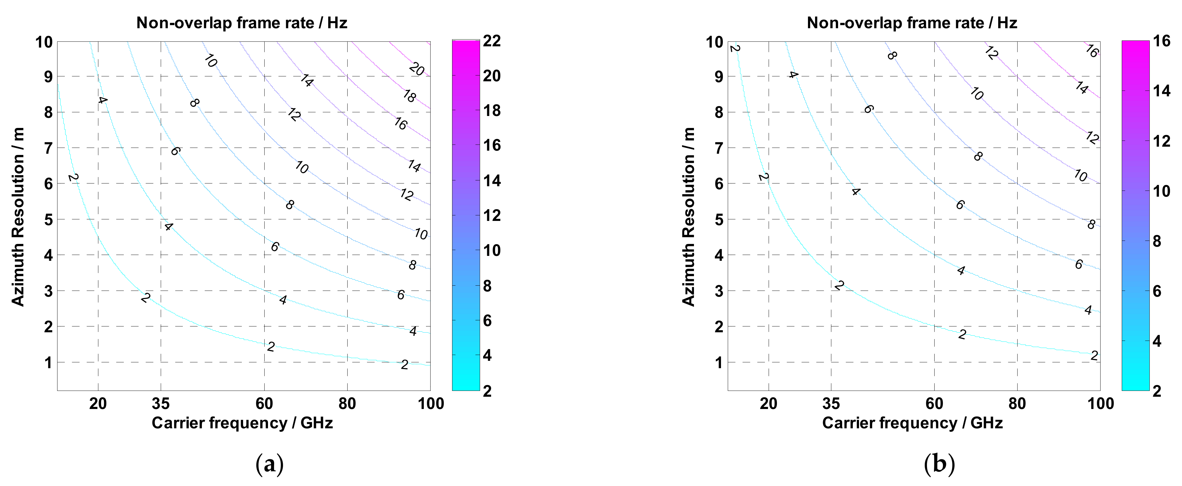
To illustrate the effect of different parameters on the frame rate, a numerical analysis is carried out. Figure 2 shows the variation of the non-overlap frame rate with the carrier frequency and azimuth resolution of a typical airborne ViSAR system. The speed is 100 m/s, the center slant range is 30 km, s. When the carrier frequency is 35 GHz and the azimuth resolution is less than 6.4 m, the non-overlap frame rate is greater than 5 Hz. Figure 3 shows the variation of the non-overlap frame rate with the carrier frequency and azimuth resolution of a typical spaceborne ViSAR system. The speed is 7271 m/s, the center slant range is 820 km, and s. When the carrier frequency is 35 GHz and the azimuth resolution is less than 2.4 m, the non-overlap frame rate is greater than 5 Hz. As the squint angle increases, the non-overlap frame rate will decrease accordingly, as is shown in Figure 2b and Figure 3b.
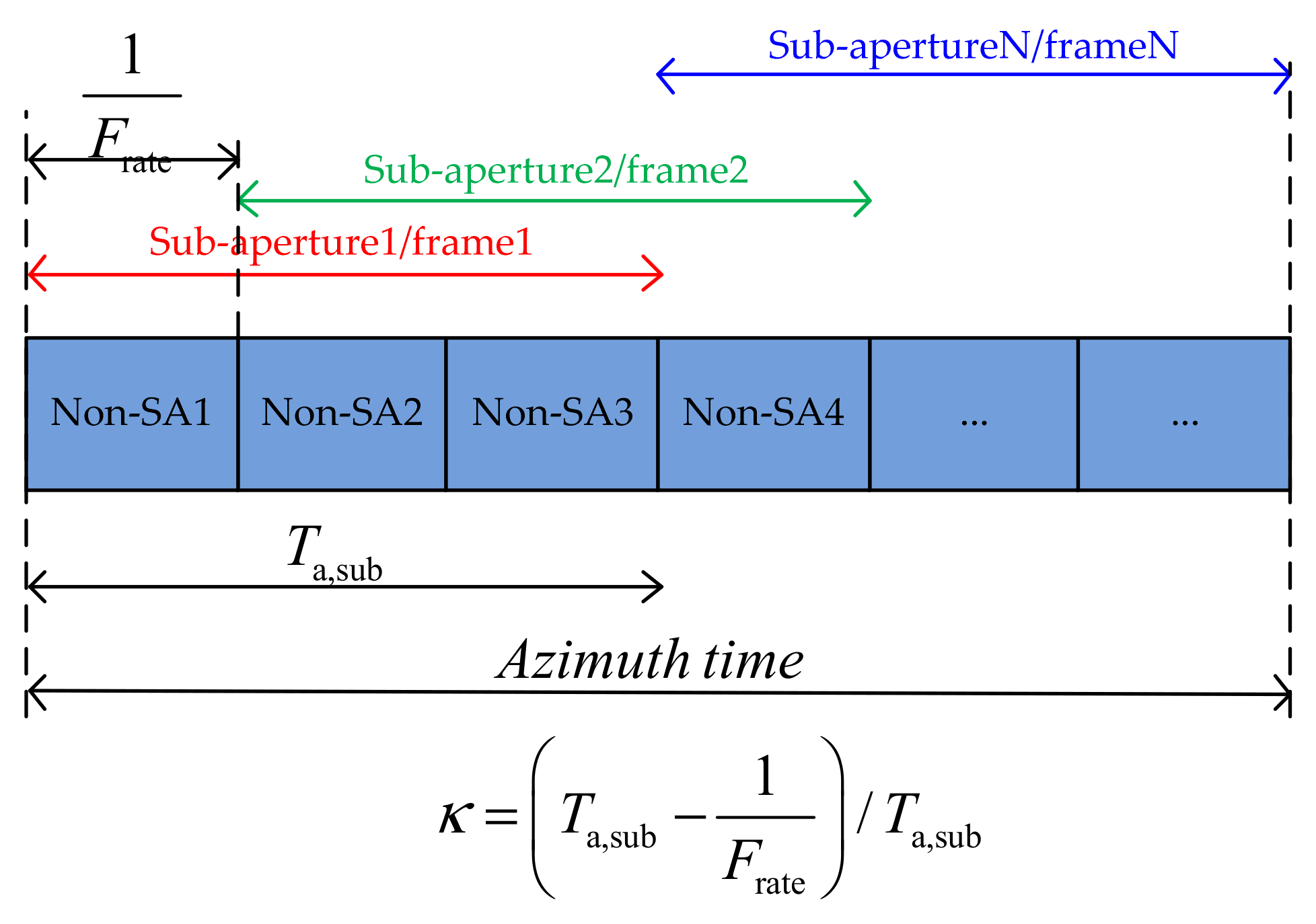
According to the above analysis, for the typical microwave band (35 GHz) SAR, it is difficult to form a high non-overlap frame rate (>5 Hz) SAR video with a resolution of less than 1 m, whether it is an airborne or spaceborne SAR system. In this case, a video sequence with a higher refresh rate can be obtained through the sub-aperture overlap, and the frame rate is defined as the overlap frame rate. Under the premise of ensuring the azimuth resolution of the ViSAR frame image, the overlap frame rate can be higher than the non-overlap frame rate, which can ensure the continuity of the moving target in the video and is more conducive to the subsequent moving target detection processing. The schematic diagram of an overlap frame rate processing is shown in Figure 4. The scene observation time is composed of N sub-aperture images or frame images, and each sub-aperture image has several non-overlap sub-aperture (Non-SA) images. The non-overlap sub-aperture images Non-SA1~Non-SA3 synthesize Sub-aperture1, and the non-overlap sub-aperture images Non-SA2~Non-SA4 synthesize Sub-aperture2. Sub-aperture1 and Sub-aperture2 all contain Non-SA2 and Non-SA3.
As is shown in Figure 4, for a given overlap frame rate and azimuth resolution , the interval between the start time of sub-aperture 1 and sub-aperture 2 is the reciprocal of the frame rate, i.e., . Thus, the overlapping part of sub-aperture 1 and sub-aperture 2 is . Combining Equation (2), the overlap ratio of the SAR image is defined as
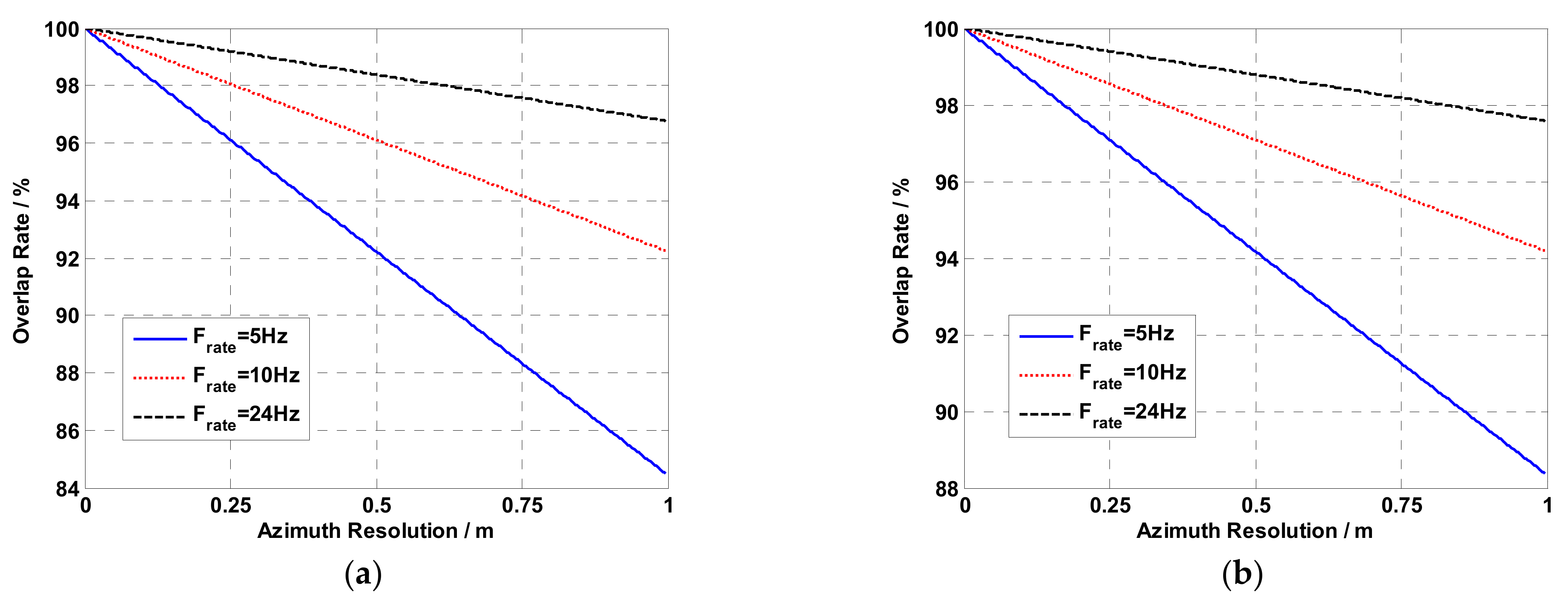
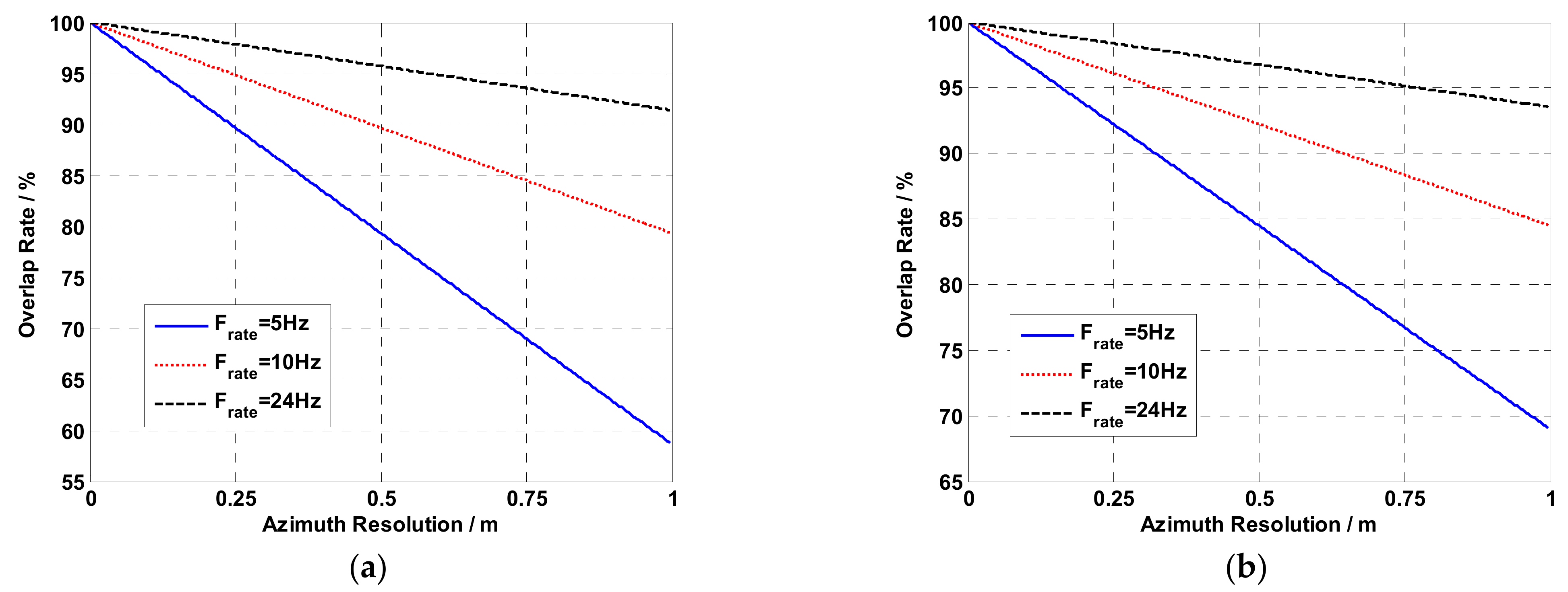
Figure 5 and Figure 6 show the variation of the overlap rate with the azimuth resolution when the carrier frequency is 35 GHz and the overlap frame rate is 5 Hz, 10 Hz and 24 Hz. Figure 5 shows the results of a typical airborne ViSAR system with a speed of 100 m/s and a scene center slant range of 30 km ( s). Figure 6 shows the results of a typical spaceborne ViSAR system, with a speed of 7271 m/s and a scene center slant range of 820 km ( s). For a given SAR video frame rate, the higher the azimuth resolution of the frame image, the greater the aperture overlap rate; under the same azimuth resolution, the higher the SAR video frame rate, the larger the aperture overlap rate; the larger the squint angle, the greater the aperture overlap rate required to form the same azimuth resolution and video frame rate. For a typical airborne ViSAR system with a 5 Hz overlap frame rate, when the frame image azimuth resolution is 0.25 m, the overlap rate is 96.11%, and when the frame image azimuth resolution is 0.5 m, the overlap rate is 92.22%. For a typical spaceborne ViSAR system with a 5 Hz overlap frame rate, when the frame image azimuth resolution is 0.25 m, the overlap rate is 89.65%, and when the frame image azimuth resolution is 0.5 m, the overlap rate is 79.31%.
2.2. SAR Video Formation Method
As opposed to the instant acquisition of two-dimensional images by the optical video system, SAR takes time to form sub-aperture images with a certain resolution and finally synthesize an SAR video. At the same time, to better detect and track moving targets, it is necessary to obtain a highly matched sub-aperture image sequence. It can be seen from the analysis in Section 2.1 that for the microwave frequency band, to form a typical high-resolution and high-frame-rate SAR video, the overlap ratio needs to range from 79.31% to 96.11%. This puts forward higher requirements for the imaging algorithm to effectively focus the sub-aperture echo and avoid repeated calculations.
The time-domain back projection (BP) algorithm is widely used in ViSAR imaging processing. This algorithm can accurately reconstruct the value of each pixel in the image and can be regarded as the inverse process of the echo collection. In principle, the BP algorithm does not have any theoretical approximation, and it can naturally solve imaging problems that are difficult to solve by frequency domain algorithms, such as track curvature, ground elevation, squint, and space-dependent motion error compensation. In ViSAR imaging processing, the advantages of using the time-domain BP algorithm are mainly that (1) It can process a SAR video with any geometric resolution and any refresh rate, and has strong flexibility: BP processing can adopt pulse-by-pulse processing; thus, it can realize image sequence imaging with any sub-aperture and any overlap rate; (2) The sub-aperture SAR image grid can be set flexibly: it can get the image grid and image sequence that change with the squint angle; it can focus on the unified coordinate grid, which can simplify the difficulty of subsequent registration processing of ViSAR; it can magnify the region of interest in real time, taking into account global imaging and local fine imaging; (3) Suitable for parallel processing: BP imaging of each pulse echo is not correlated with each other and the computational load is equivalent, which facilitates parallel computing and real-time processing.
The basic principles of the time-domain BP algorithm are to set the grid of the image to be generated, obtain all the echoes corresponding to the corresponding pixels of the grid in the two-dimensional time domain after the range pulse compression, and perform coherent superposition to obtain the final image after the echo is compensated for the residual phase.
Ignoring the scattering complex coefficients and the weighting of the antenna in the elevation and azimuth directions, the signal after the range pulse compression can be expressed as
where is the slow time number of echo sequence, is the fast time number of echo sequence, is the transmitted signal bandwidth, is the speed of light, and represents the slant range from the antenna phase center to the point target.
In the BP imaging process, the flight trajectory of the sensor and the illuminated area of the radar beam are unified under the same coordinate system, and the image grid of the imaging area is set according to the geometric relationship of the scene , where is the azimuth number of image and is the range number of image.
Furthermore, the distance between the antenna phase center and the image grid can be calculated for each azimuth time . Suppose the number of azimuth echo signal is and the number of range echo signal is , then the SAR pixel value at the image grid can be obtained after coherent superposition according to the following formula
where represents the SAR image of the mth echo mapping, which can be calculated by
where represents the mapping weight, which takes a value of zero during the antenna beam irradiation. The pulse-based BP realization process is shown in the Figure 7. The detailed description of the BP algorithm can be found in the literature [24,25,26,27].
The main disadvantage of the BP algorithm is the large amount of calculation and low efficiency. To reduce the computational complexity of the algorithm, a series of modified BP algorithms have been developed, such as fast hierarchical back projection (FHBP), local back projection (LBP) and FFBP and so on. Among them, the FFBP algorithm can theoretically achieve the same order of efficiency as the frequency domain imaging algorithm and can achieve both imaging accuracy and efficiency [24]. This paper adopts the time domain FFBP to realize the ViSAR sub-aperture echo imaging processing and the video generation processing. Moreover, considering the high overlap rate of the microwave band SAR video, in order to simplify the processing flow of forming the SAR video and avoid repeated calculations, this article draws on the method of shift register and adopts an efficient processing method based on FFBP for ViSAR video formation.
For a given SAR video frame rate (), the number of echo points corresponding to the non-SA image can be expressed as
where stands for rounding down.
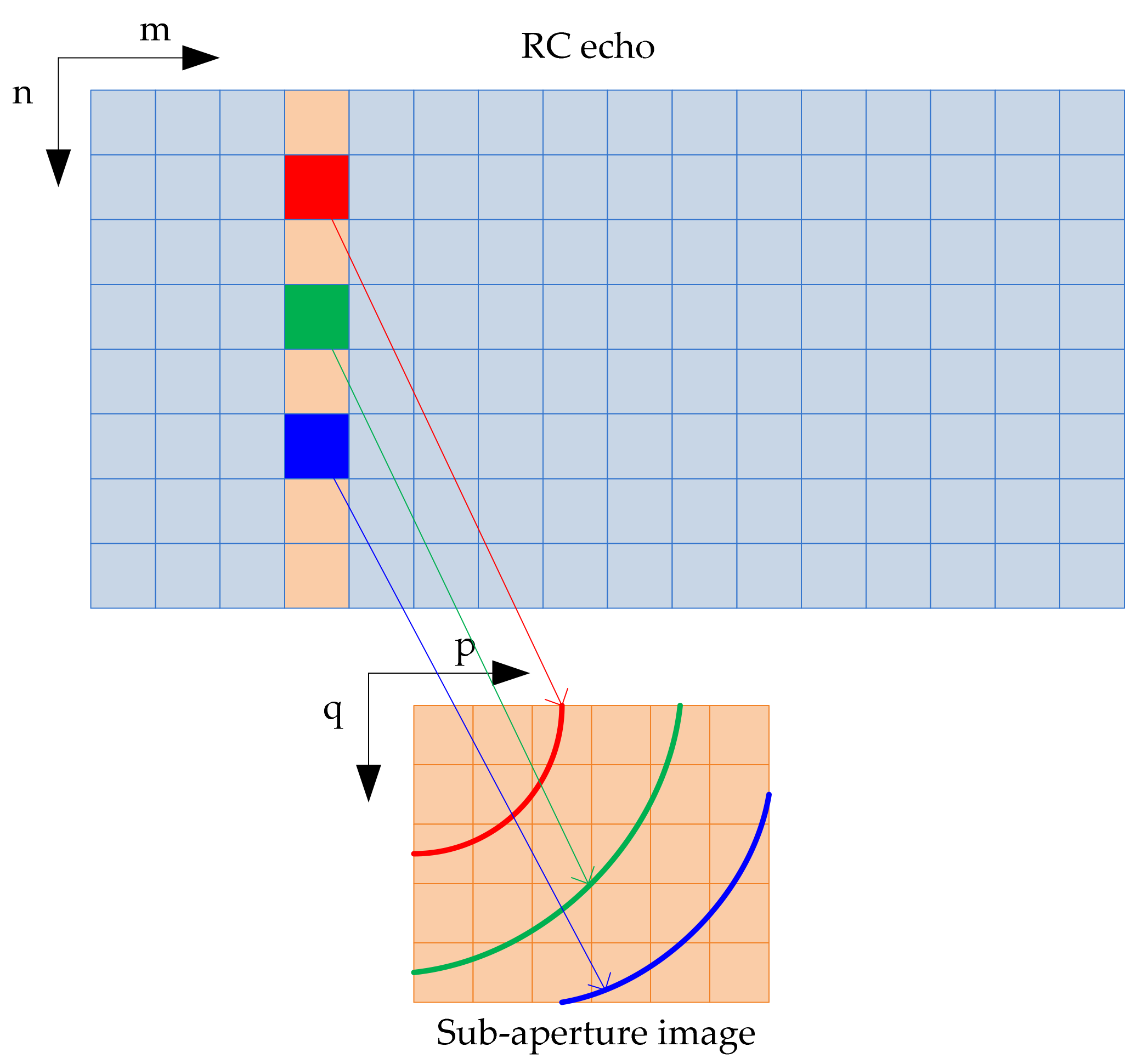
The FFBP algorithm is used to map the non-overlapping echoes into the same imaging grid, which avoids the process of matching the images of different squint angles to the same imaging grid after the frequency domain algorithm imaging processes. Using the FFBP algorithm to perform fast imaging processing on the divided sub-apertures, the overlapped frame images can be obtained by
where ,. Since the FFBP imaging of each sub-aperture is independent of each other, for computers with multi-core resources, parallel processing can be used to improve the computing efficiency. The overlap frame rate can be calculated according to Equation (4), and then the number of overlap frame images for coherent accumulation can be expressed as
where represents rounding up. Because the BP imaging algorithm is the realization of the coherent accumulation process, it can simulate the way the shift registers to form an SAR video frame image, which can effectively avoid repeated calculations. The calculation formula for the first frame of image is
The recursive calculation expression for forming the kth frame image is as follows:
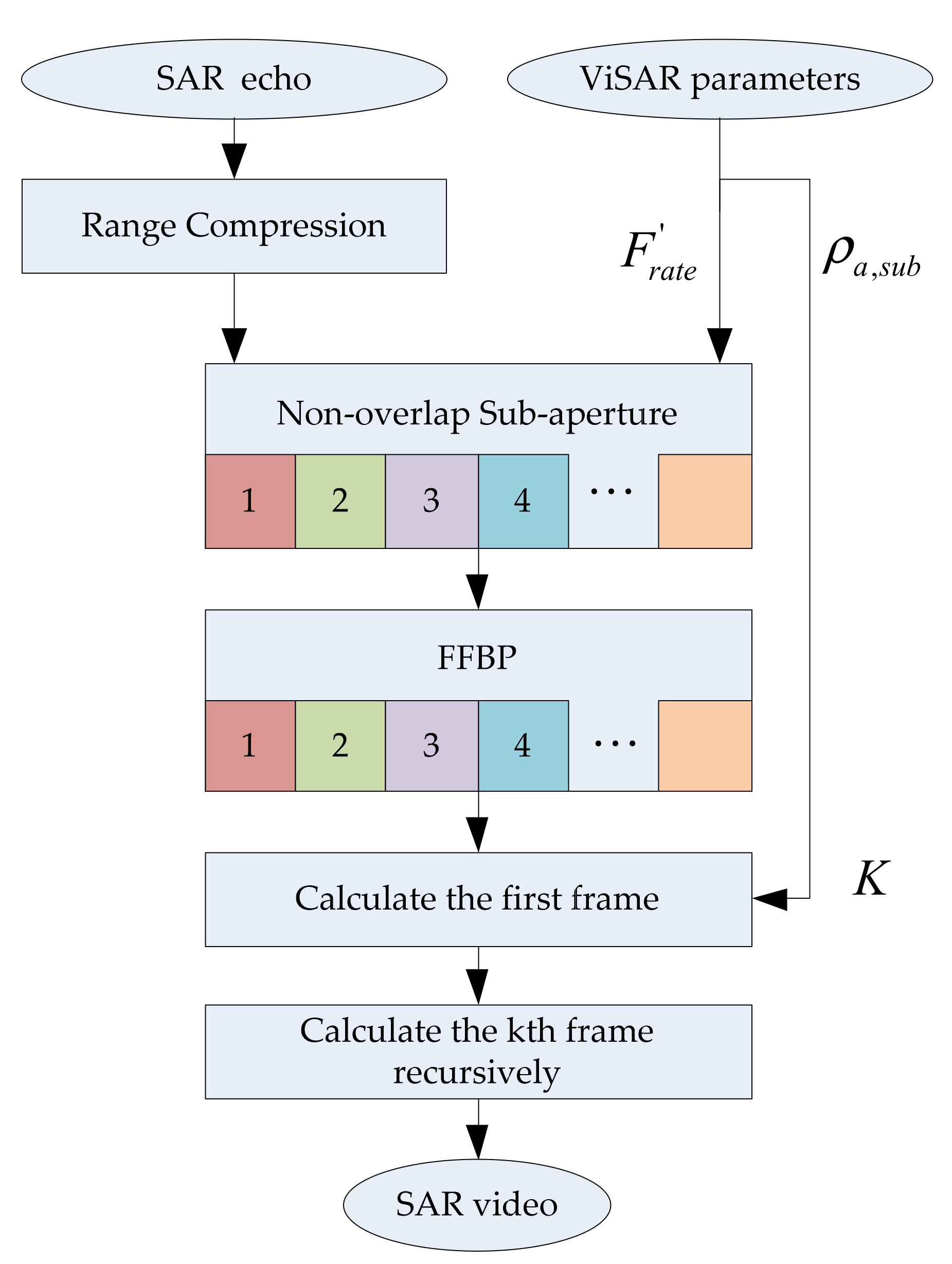
The processing flow of efficiently generating a video stream based on FFBP-based shift register is shown in Figure 8. The processing flow is as follows:
Step 1: According to the specified SAR video frame rate , divide the non-overlap sub-aperture, reference Equation (8). The FFBP algorithm is used to perform imaging processing on each non-overlap frame image, and each non-overlap sub-aperture image complex data is obtained.
Step 2: Calculate the number K of overlap frame images to be merged according to the azimuth resolution of the given SAR video frame image. Calculate the first frame complex image .
Step 3: Use the frame image recursive calculation Equation (13) to obtain each frame image , then construct the SAR video from the obtained frame image sets and complete the formation of the SAR video.
The maximum number of non-overlap sub-aperture images needed to be stored is K, which has the advantages of small calculation amount and low storage requirement.
3. Moving Target Shadow Formation
3.1. Mechanism of Shadow
Moving targets such as ground vehicles show obvious shadow features in ViSAR sequences. Figure 9 shows the shadow features of ground moving car shown in real ViSAR image from Sandia National Laboratory (SNL), showing the ViSAR footage of a gate at Kirtland Air Force Base. (http://www.sandia.gov/radar/_assets/videos/eubankgateandtrafficvideosar.mp4, accessed on 1 August 2021). When the vehicle stops, the target energy is well focused and only the shadow can be observed. When the target moves, it defocuses and the defocused image deviates from the original position. However, because the electromagnetic wave cannot irradiate the vehicle position, it will form an obvious shadow feature at the vehicle position. It is shown that the shadows moving along the road are always at the actual physical location of vehicles, which can be used for ground moving target detection. However, the shadow characteristics of moving targets are closely related to SAR system parameters, moving target size and velocity, ground background scattering characteristics and other factors. This section analyzes and deduces the shadow formation mechanism and conditions of moving targets, and obtains the speed limit conditions of shadow formation of moving targets. The analysis results can support ViSAR system parameter design and data processing parameter setting.
Like the light source, the radar at any instantaneous sampling moment can be regarded as a point power source. Figure 10 shows an obstacle’s shadow of radar at a certain sampling position. The light gray region represents local shadow sheltered by the target bottom and the dark gray region represents the obstacle’s shadow under the illumination of radar.
Assume that the background is zero-height, the shadow of moving target is its surface projection under the illumination of radar. Define that the radar position is , and the coordinates of the obstacle’s surface at the moment are given as follows:
where represents the obstacle surface, represents the set of obstacle surfaces, is the number of samples at the obstacle surface. The instantaneous vector from the radar to the obstacle surface is as follows:
The shadow projected on the ground can be expressed as
Equation (15) is the expression of obstacle shadow at arbitrary moment. And Equation (15) is also the signal foundation in the simulation of moving target. For low height targets, such as car, tank and mini-bus, the extra shadow (shown in Figure 10) caused by shelter can be neglected. In the following discussion, we just take local shadow into account.
3.2. Analysis of Ground Moving Target Shadow
In an SAR image, the signal-to-noise ratio (SNR) of a static point target can be expressed as [23]
where and are the gains of transmitted and received antennas, respectively. is the radar transmitted power. We define that equals to . represents the illuminating time of scatterer P without the shelter. is the carrier wavelength. is the RCS of target. is the nearest range between radar and target. is the Boltzmann constant and is system the loss factor. is the effective noise temperature in receiver. is the spectrum density of effective noise and is the noise coefficients of the receiver. is the pulse width. The radar flies with a velocity . and are the improvement factor of range and azimuth dimensions, respectively. They can be expressed as follows:
where is the transmitted pulse bandwidth, is the azimuth resolution. For area targets, their effective RCS can be expressed as
is the normalized RCS in the specific area. is the range resolution. is the incidence angle. And the SNR of the area targets can be expressed as
And the target power in SAR image can be given as follows:
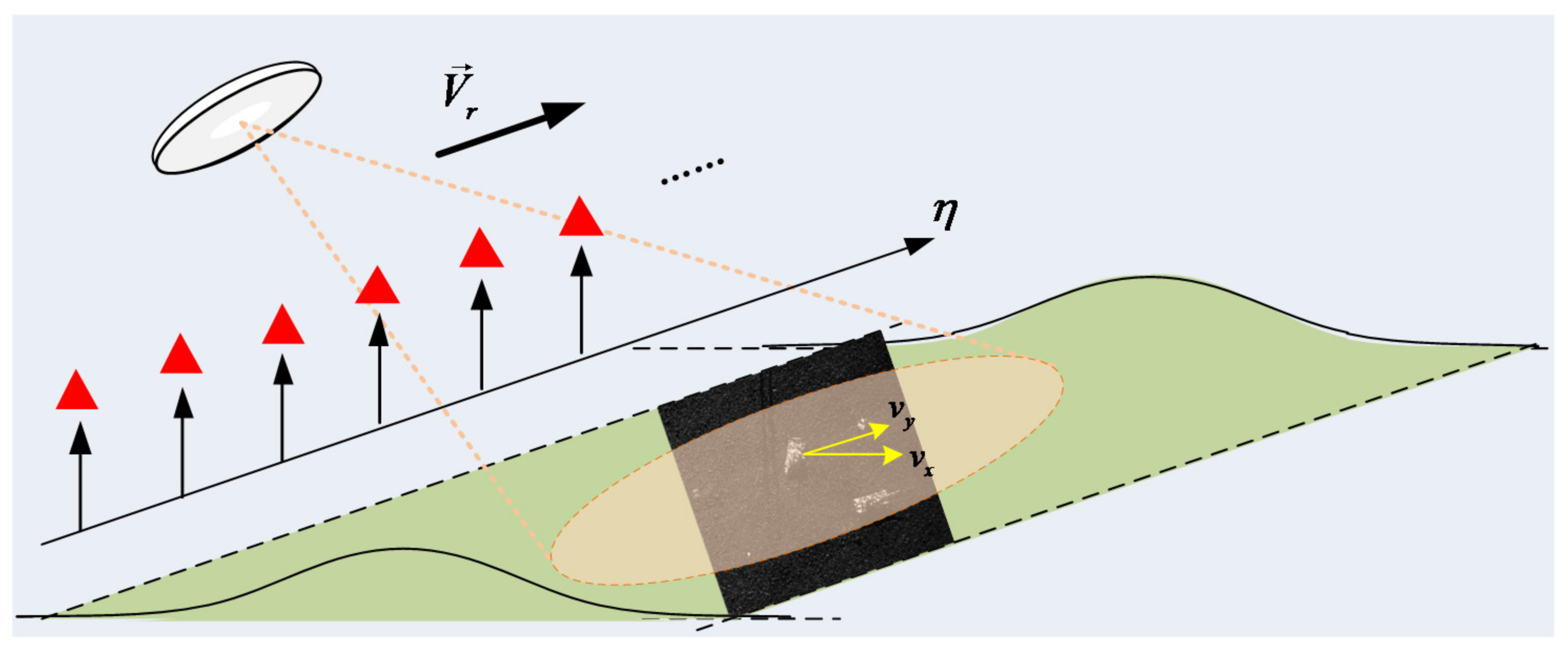
Figure 11 shows the schematic view of a moving target. Assume that the X-axis and Y-axis are the range and azimuth direction, respectively. According to [28], the velocities of the moving target along the range and azimuth dimensions have different impacts: the velocity in azimuth dimension causes the mismatch of frequency modulated (FM) rates which leads to the azimuth defocusing; the velocity along range dimension makes the focusing position deviate from the ideal azimuth position. This deviation can be expressed as
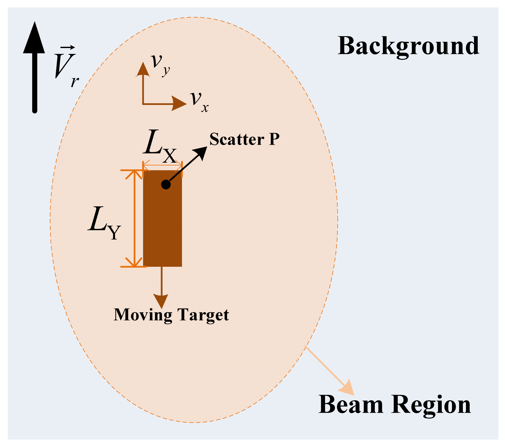
is the range velocity of moving target, and is the azimuth deviation. Figure 12 shows the relative motion between the beam illumination and moving target motion. Assume that the size of target along the range and azimuth dimensions are and , respectively. Hence, the sheltering time of scatterer P in the scene can be expressed as
Figure 11.
Schematic view of a moving target.

We define that the coefficient equals to . Ignoring the influence of other scatterer impulse response function (IRS), we discuss the power of scatterer P in SAR image in the following cases.
Case 1:
This case means that the scatterer P is partly sheltered by the moving target. And its illuminating time can be given as
Accordingly, the azimuth improvement factor can be expressed as
The power of scatterer P or Equation (20) can be rewritten as
Case 2:
In this case, the scatterer P is covered by the moving target during the whole beam illumination. Hence, the azimuth improvement factor equals to zero. And the power of scatterer P in SAR image is given as follows:
For a moving target, the prerequisite of shadow formation is that the target have a velocity component along range dimension. And its limitation can be obtained from the following formula:
Define the factor as the ratio of the average power of the shadow area to the average background power.
As the target moves with an extra azimuth velocity, it should meet the following limitation:
is the threshold that can clearly distinguish the shadow and background. In this paper, the JPEG format is adopted in the formation of ViSAR frames. is close to 0.5. In a focused SAR image, the ratio is far greater than 1. Hence, combining Equations (27) and (29), we can get the limitation of moving target shadow formation in ViSAR:
Taking an observation of Equation (30), it can be calculated that the limitations of the moving target shadow formation in ViSAR are related to the azimuth resolution of the image, the velocity of the platform, the size of the moving target, the carrier wavelength, the nearest range and the threshold.
3.3. Shadow-Based Ground Moving Target Detection
Based on the analysis of the shadow formation mechanism and the shadow formation conditions of moving target, the shadow of the moving target has the following remarkable characteristics: (1) In contrast to the defocus and displacement characteristics of the moving target in the SAR image, the shadow position is consistent with the real position of the target, which is the precondition of moving target detection in ViSAR. Based on the shadow, (2) both the stationary target and the moving target have the shadow feature. The target shadow of the stationary target is the highlight of the focus. The stationary target and its shadow region generally appear at the same time, while the moving target shadow has no such feature. The shadow formed by the stationary target is the combination of the target shadow and the projected shadow, (3) As opposed to the optical shadow formation mechanism, typical ViSAR needs 0.2 s synthetic aperture time (corresponding to ViSAR frame rate of 5 Hz) to form a frame image. The shadow is related to scattering characteristics, illumination time, imaging geometry, target size, processing parameters, etc., and has dynamic characteristics; sometimes even moving targets do not form obvious shadow characteristics. Nevertheless, this peculiar shadow is not a reliable feature, which varies continuously with the scattering properties, synthetic aperture time and imaging geometry.
Based on the analysis of the characteristics of moving target shadow image in ViSAR, a moving target shadow detection method based on sequence image change detection is proposed in this paper. The basic idea is to make full use of the time information of sequential image of ViSAR based on the high matching sequential image of the same scene obtained by ViSAR. Through the background difference, frame difference, frame difference, frame difference morphological filtering and early warning suppression are used to realize the robust detection of shadow area.
The peculiar shadow mechanism will cause variations in the shadow shape, covering area and gray value, etc. Furthermore, relatively to the vast area that ViSAR imaging generally covers, moving targets usually hold very tiny regions and can be easily missed in detection procedure. The existing shadow-based methods are highly susceptible to background noise, target energy shift, vibrational viewpoint and geometric deformation. Such phenomena are inevitable to some extent, causing numerous false alarms and a poor detection effect.
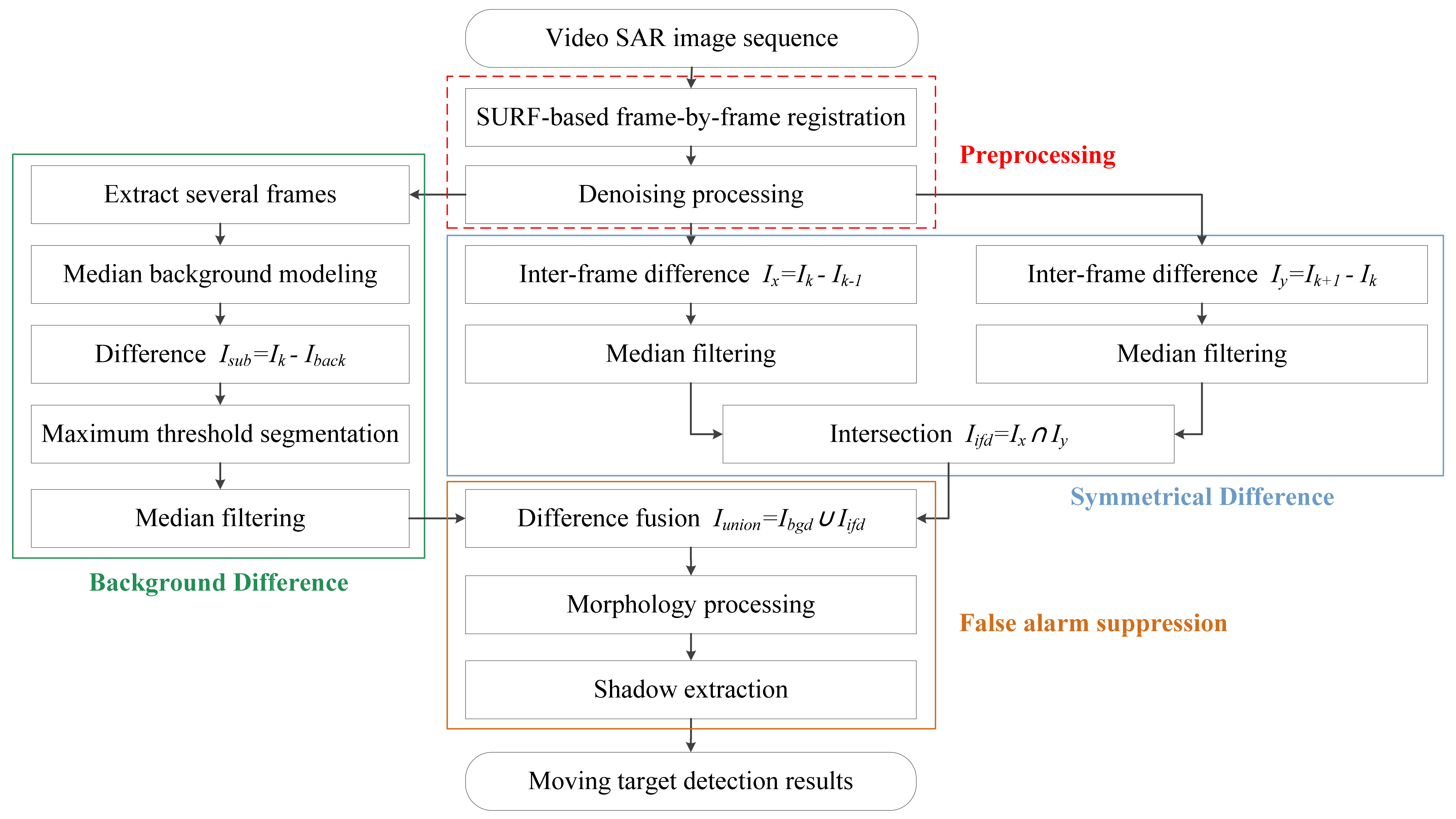
The shadow-based ground moving target detection method proposed are summarized in the flowchart shown in Figure 13. The red block highlights the preprocessing procedure and the green one circles the background difference. The symmetrical difference is surrounded by a blue rectangle and the false alarm suppression is highlighted by an orange one.
The preprocessing procedure includes registration and denoising processing. The registration process can reconstruct the correlations among adjacent frames by spatial transformations. Otherwise the vibrational background will be regarded as moving objects in an unregistered SAR video. The sped-up robust features (SURF) algorithm, as a recent feature-based registration algorithm, is introduced to register ViSAR image sequence, which significantly outperforms other algorithms in both accuracy and robustness, and has unique advantages in calculation speed [29]. The speckle noise and thermal noise present in ViSAR images may seriously corrupt the detection effect and cause a large number of false alarms. Thus, a denoising processing method, such as the V-BM3D algorithm [30], is introduced to suppress various noises in ViSAR images.
In this paper, we introduce the background difference and symmetric difference method into ViSAR MTD. Compared with other shadow detection methods, such as the deep-learning shadow detection method, it has the advantages of fast calculation and good robustness. The background difference method is a traditional method for video MTD, which extracts a motion region by thresholding the difference between the current frame and the background template. The symmetrical difference operates an inter-frame difference on the two frames adjacent to the current one, and fuses their results together. In general, the symmetrical difference will extract the edge information of targets. Then, the difference fusion procedure is used to fuse the results of these two methods and obtain their union as the final extraction result. This fusion method could expand the covering area of moving targets and increase the discrimination between the target and background, hence improving the extraction effect. The remaining false targets can be eliminated by subsequent morphology processing. Such processing could eliminate some remaining small-size false alarms, yet do no damage to moving targets in the meantime.
4. Experiment Results and Discussion
4.1. Uniform Scene Simulation
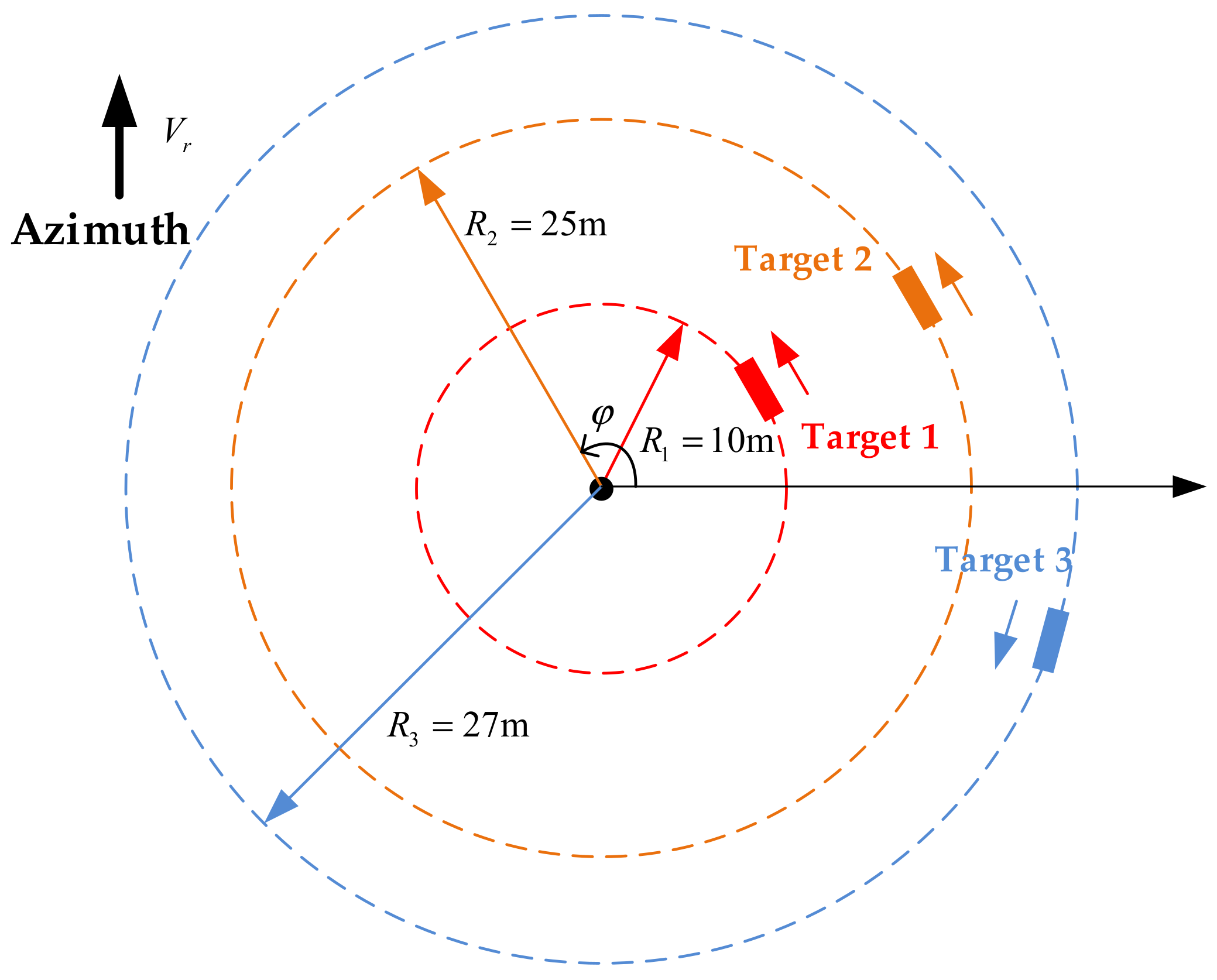
To verify the validity of Equation (30), three experiments were designed with Ka band and spotlight mode. The experimental scene is given in Figure 14. Three targets move with a same constant angular rate at different radiuses. The radiuses are [10 m, 25 m, 27 m], respectively. The targets size is 5 m × 2 m (). We define that the range dimension is the zero-radian path and the positive angle orientation goes counterclockwise. is the target rotate angle. The experiments parameters are given in Table 1.
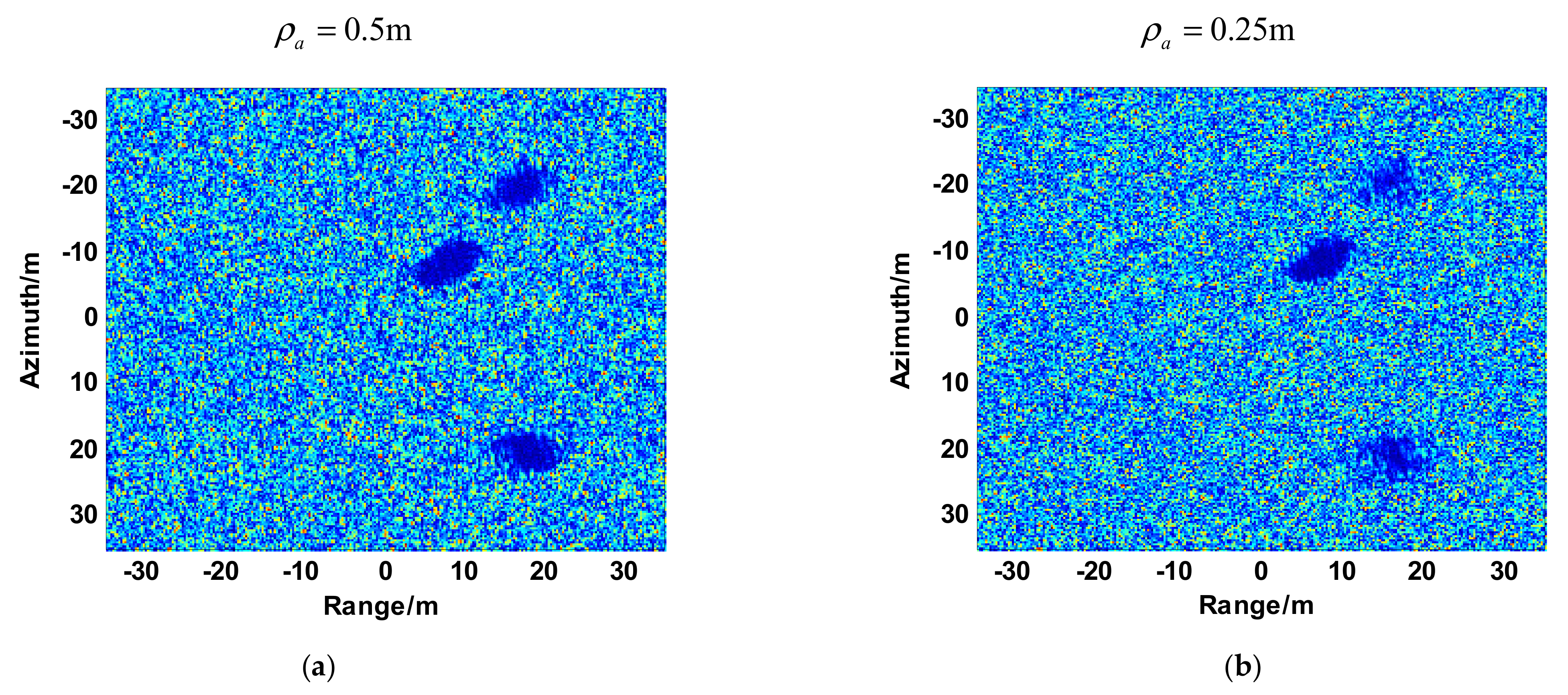
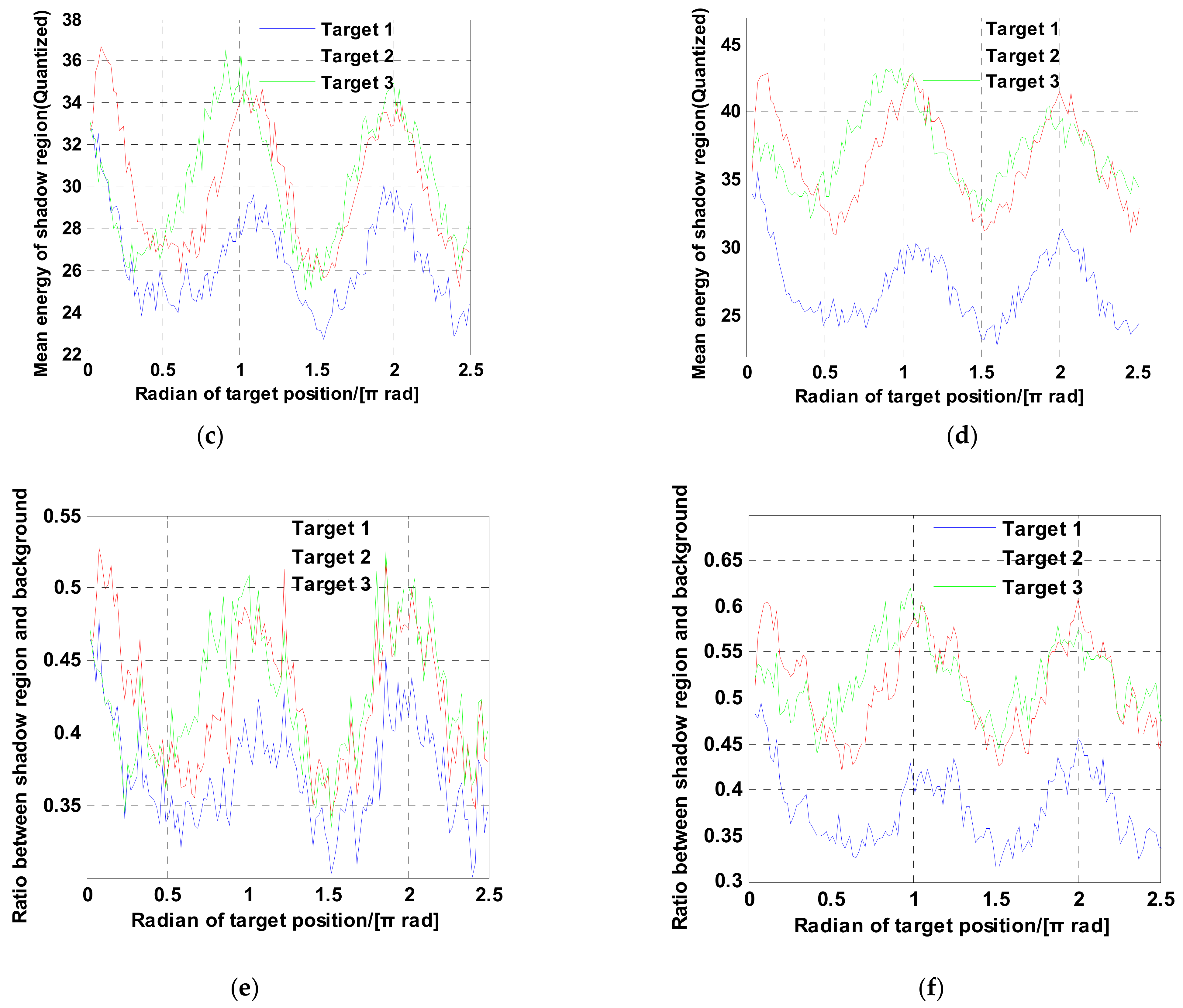
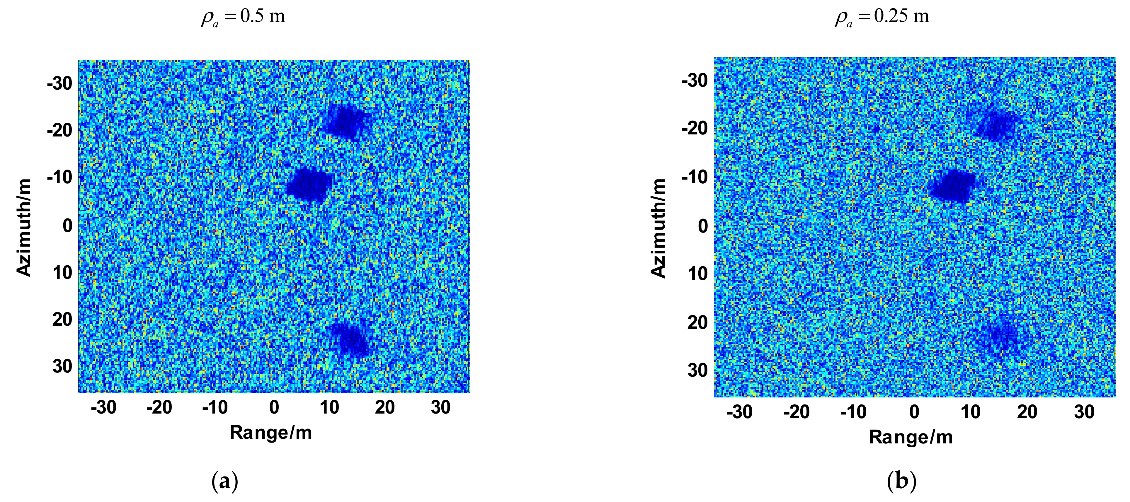
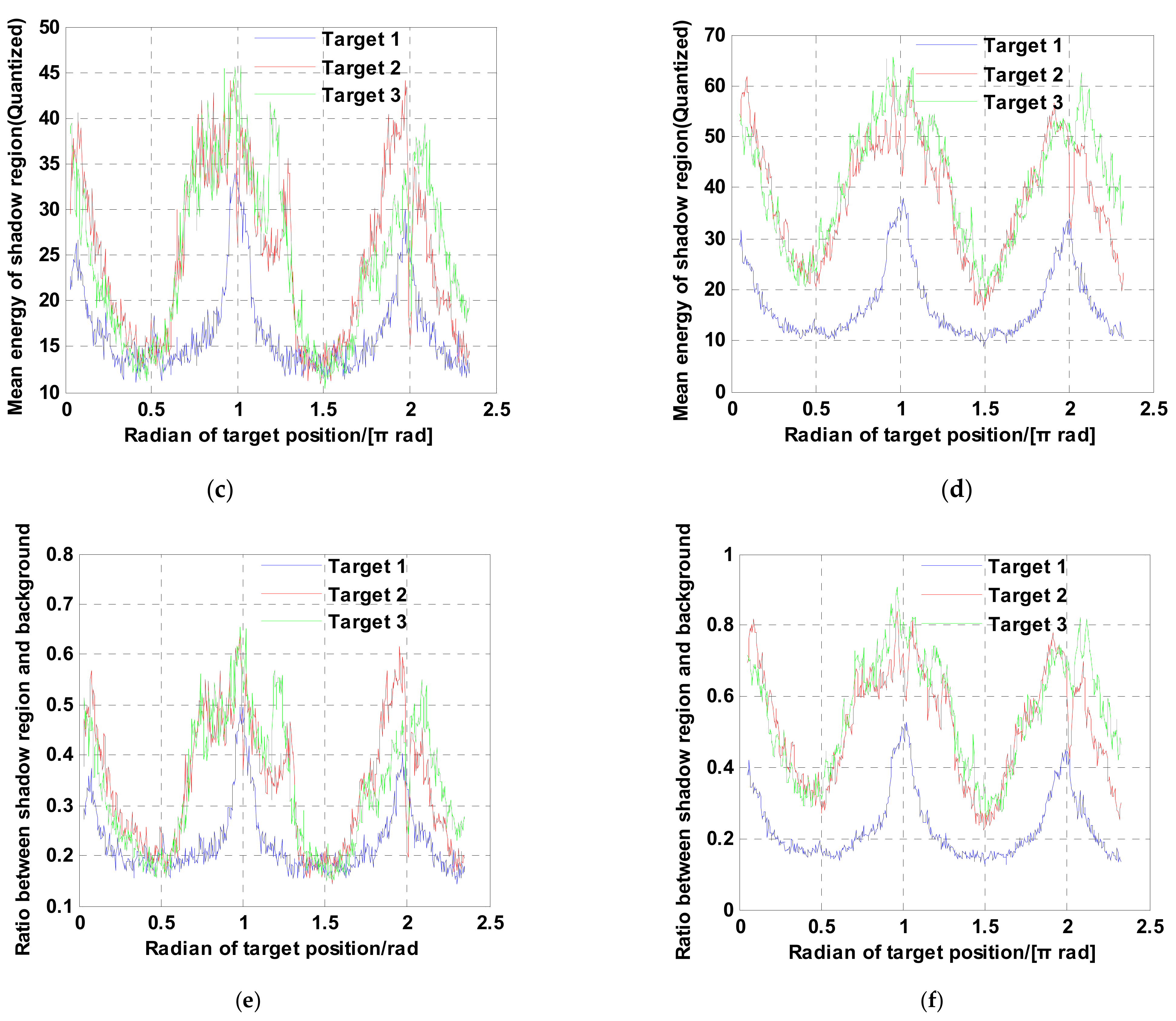
Figure 15, Figure 16 and Figure 17 are the results of experiment 1, experiment 2 and experiment 3, respectively. Compared to Figure 15, Figure 16 and Figure 17, it is obvious that the finer the azimuth resolution is, the harsher the moving target formation becomes. Figure 15a,b and Figure 16a,b show that the range between the radar and the scene also limits the moving target shadow formation velocity. Figure 15a,b and Figure 17a,b reveal that the velocity of the platform also plays an important role in the formation of the moving target shadow. The above phenomena validate the validity of Equation (30). From the statistical result of the mean shadow energy shown in Figure 15c–f, Figure 16c–f and Figure 17c–f, we can see that the maximum mean energy appears at the rotate angle . The reason for this phenomenon is that the range dimension velocity of the moving target appears to be zero while the rotate angle equals to . This means that no azimuth offset exists and the energy of the moving target gathers around its real azimuth location. Hence, the mean energy is the maximal when the rotate angle equals to . For a target with a strong RCS, the shadow cannot be shaped at this moment. In contrast, the mean energy is minimal at the rotate angle . The azimuth focusing offset achieves the maximum while the rotate angle equals to in the uniform circular motion. The energy of the moving target gathers around the offset position and the mean energy of the shadow region is smaller than the mean energy at any other rotate angle in the uniform circular motion.
4.2. Real Data Simulation
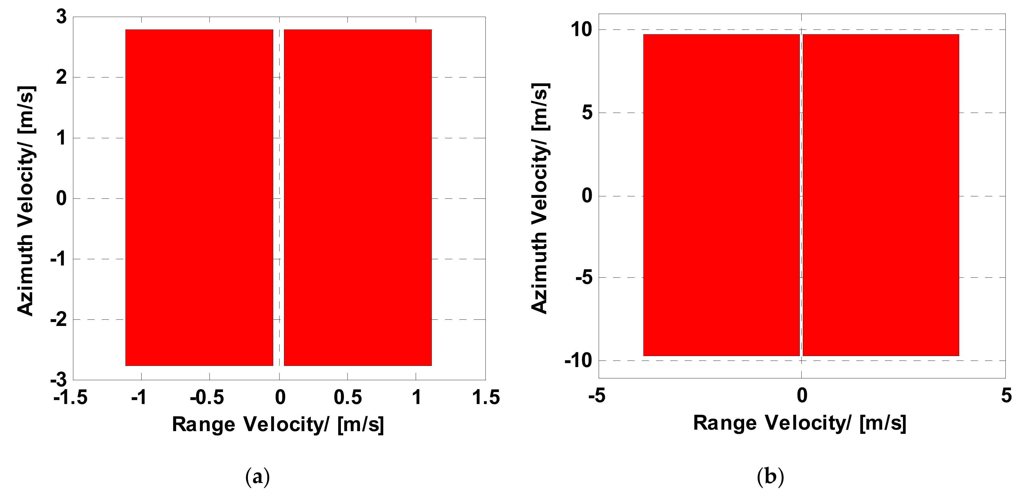
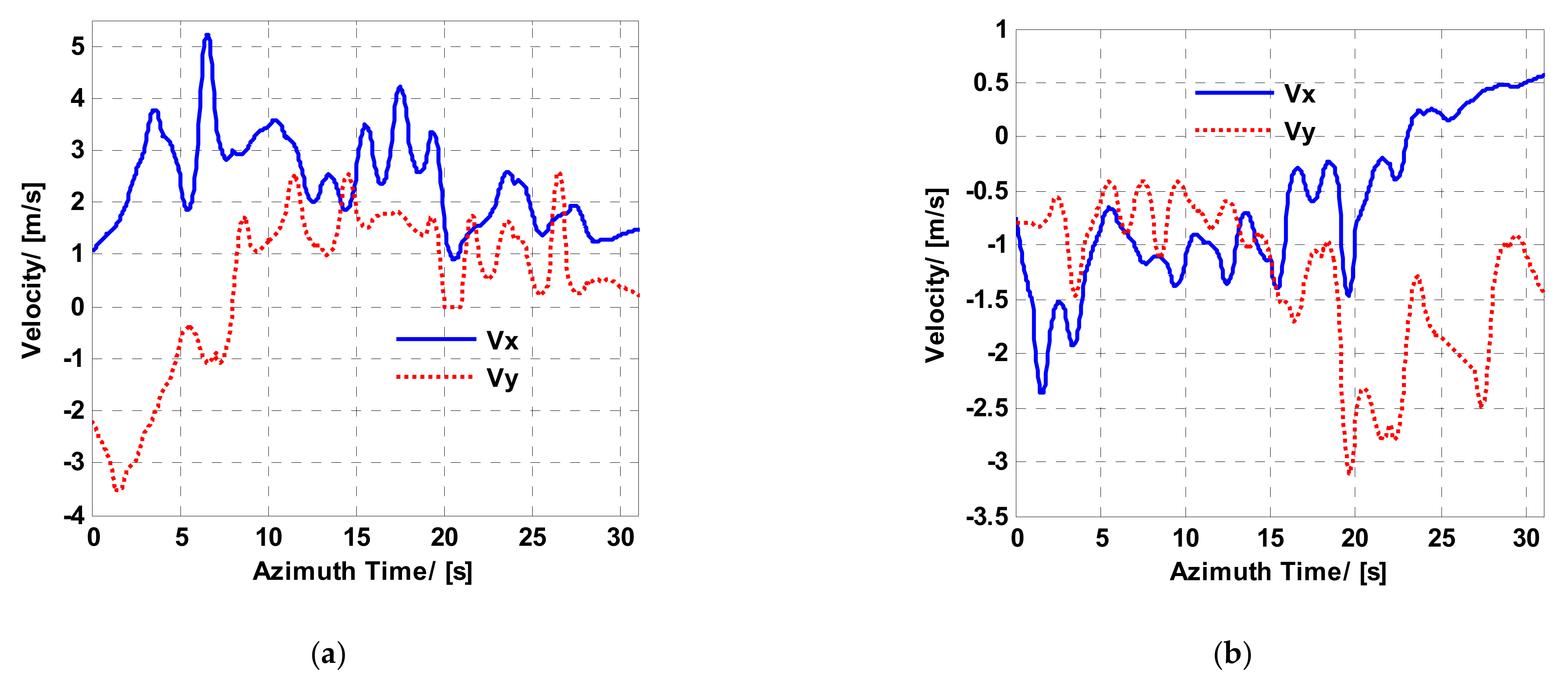
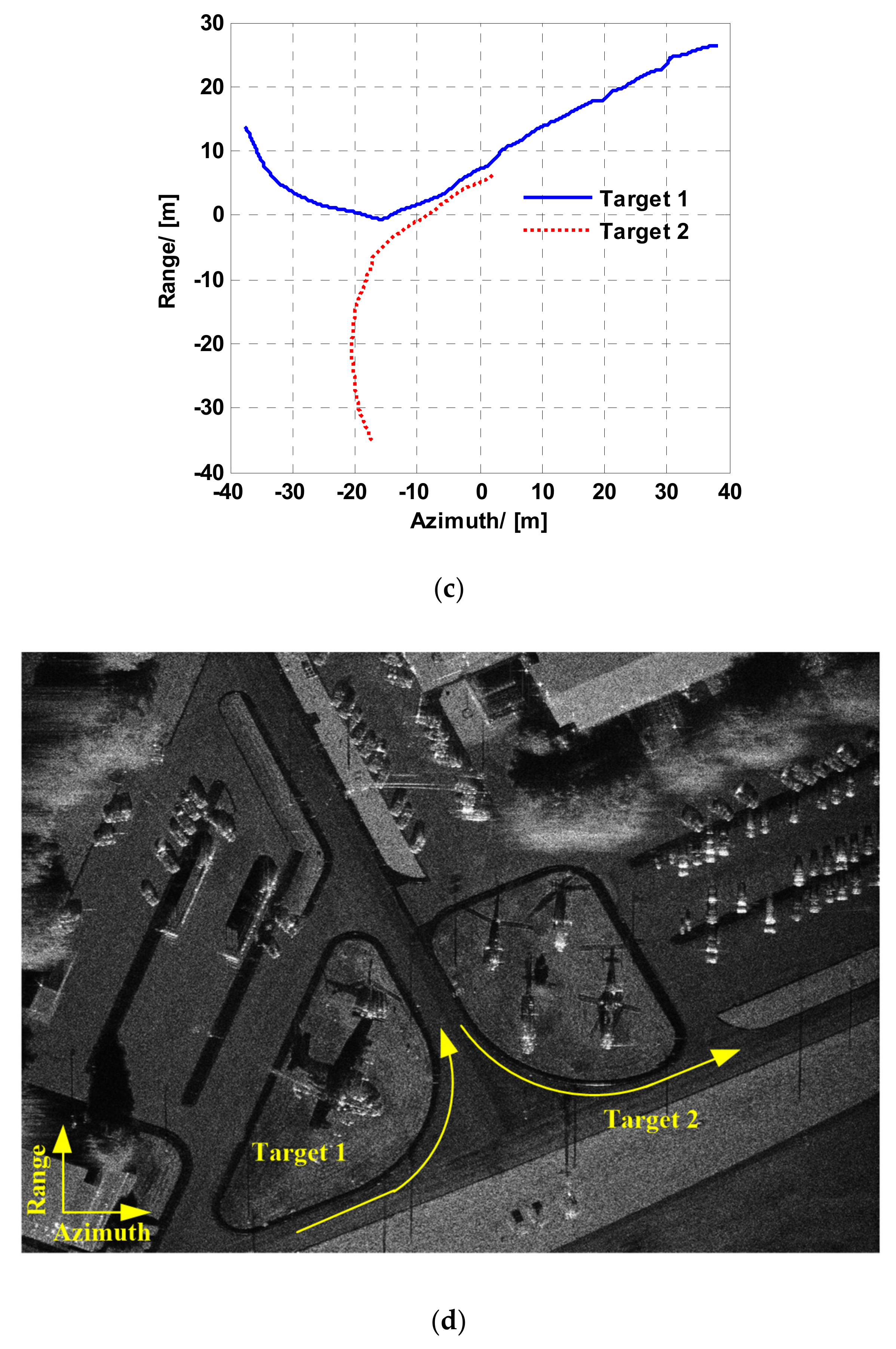
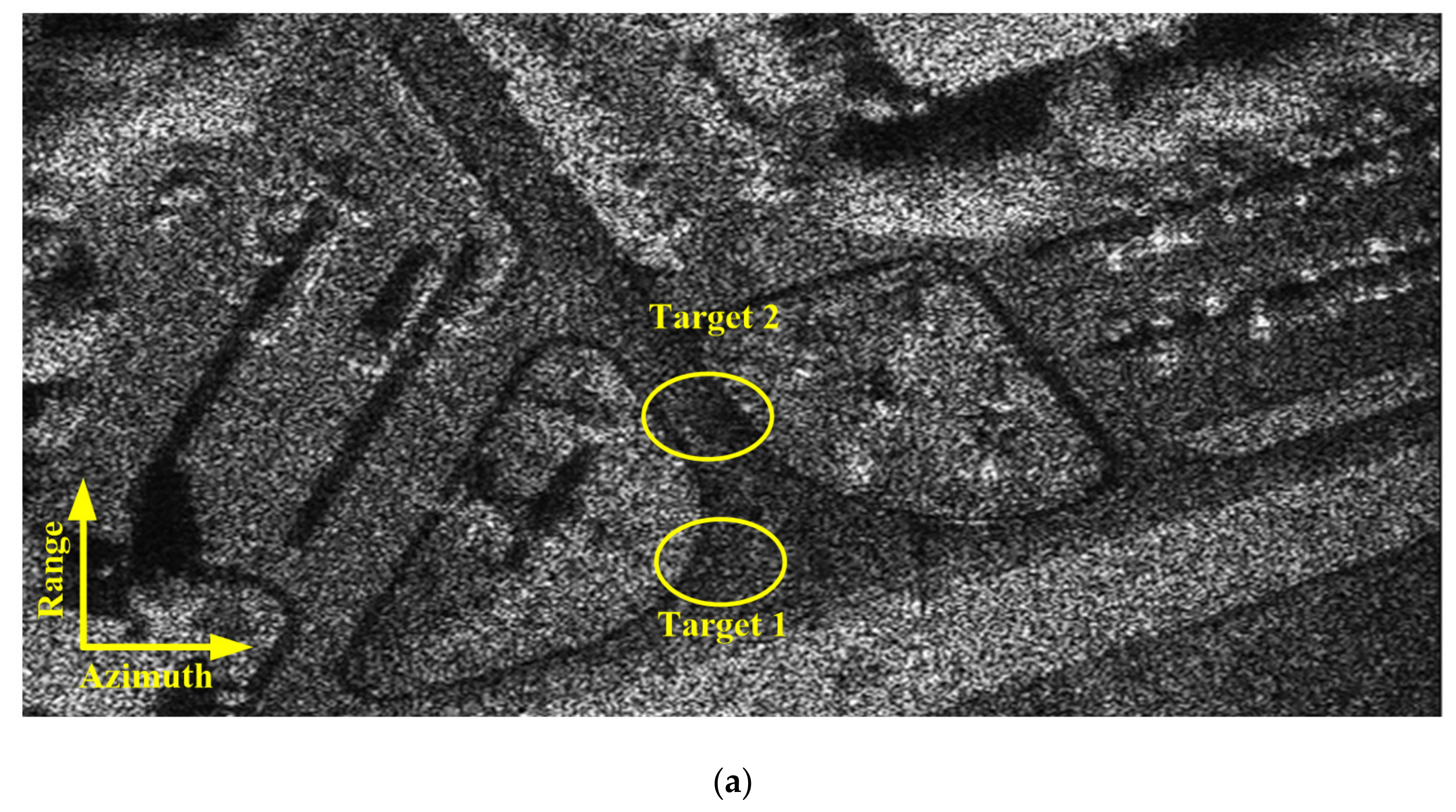
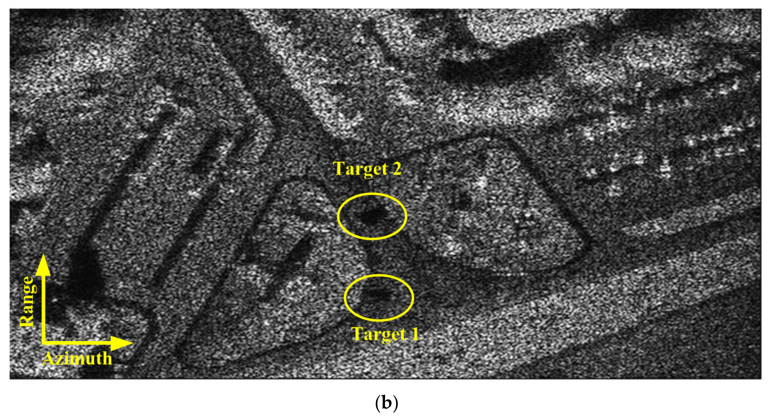
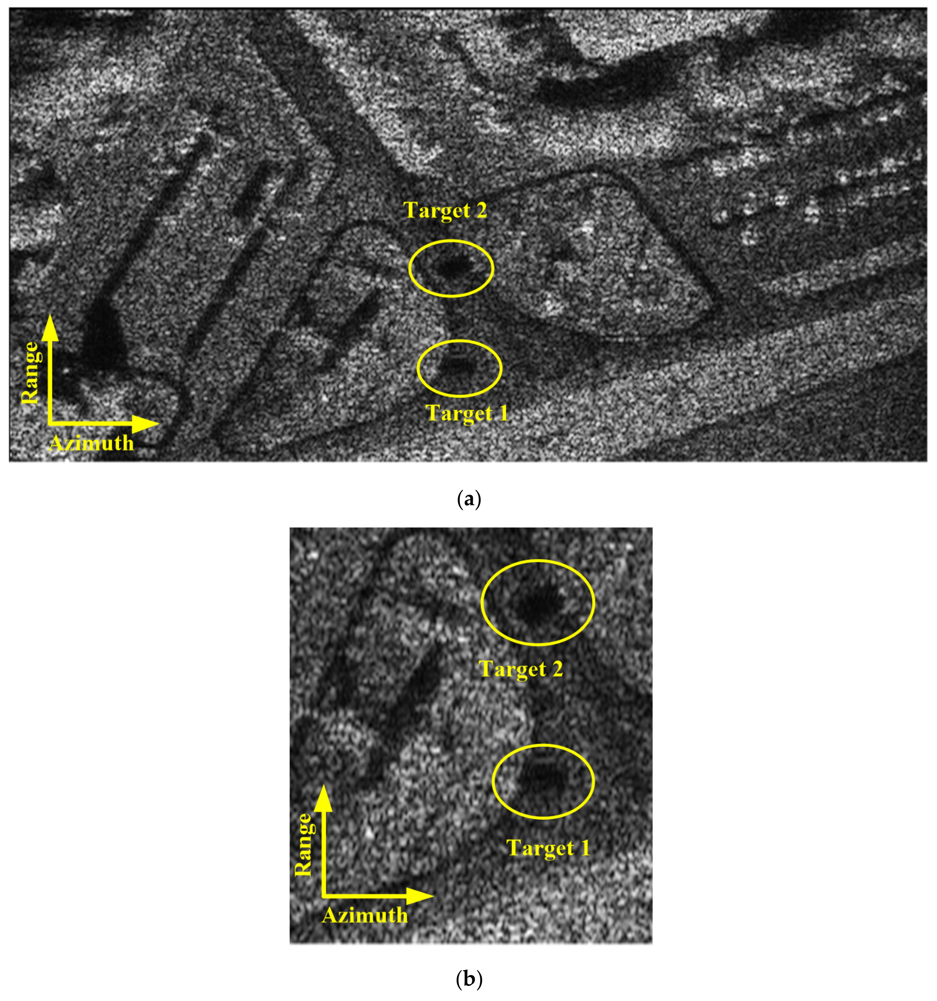
To further prove the validity of the analysis, this paper also shows the simulated natural scene. According to the point scattering model, the single look data of the SAR image can be regarded as natural scene’s electromagnetic backscattering coefficient [31,32]. A high-resolution real Ka-band SAR image (https://www.sandia.gov/radar/complex-data/, accessed on 1 August 2021) whose resolution is 0.1 m × 0.1 m (range × azimuth) is used to simulate the ViSAR echo of the natural scene. X-band and Ka-band experiments are carried out in this paper. Two moving targets are added to the simulations. The simulation parameters are given in Table 2. According to Equation (30) and Table 2, Figure 18a,b shows the moving target velocity and the velocity limited regions of X-band and Ka-band. The comparison of Figure 18a,b demonstrates that the region of velocity limitation based on the shadow detection gets larger while the carrier frequency becomes larger. In Figure 19a,b, the blue rigid and red dashed lines represent the azimuth and range velocities of target 1 and target 2, respectively. Figure 19c shows the trajectories of the two moving targets. Figure 19d shows the simulation background and the directions of two moving targets in the simulation. And in the X-band experiment, the moving target shadow is almost indistinct in all X-band ViSAR frames. In the Ka-band experiment, the shadows of the added moving targets are obvious in most Ka-band ViSAR frames. The ViSAR formation results of the simulated experiment are given in Figure 20.
Figure 20 and Figure 21 show the X-band and Ka-band results of a full and localized scene, respectively. The azimuth resolution of the simulated results is 0.5 m. The shadows of moving target are obviously in the simulated result of Ka-band experiment. And the shadows of the moving target are difficult to be distinguished from the background in the simulation result of X-band experiment. The simulated results reveal that the shadow of the moving target is more easily formatted while the carrier frequency is larger. To further discuss the validity of Equation (30), we also perform a Ka-band simulation in which the receiver is mixed with thermo-noise. The other parameters are the same as those listed in Table 2. Figure 22a,b shows the whole and localized results of Ka-band simulation, whose receiver is mixed with thermo-noise. The comparisons of Figure 20b and Figure 22a, Figure 21b and Figure 22b demonstrate that the thermo-noise has little effect on the moving target shadow formation. The real data simulation results also prove the validity of Equation (30).
5. Conclusions
ViSAR is a new application in the radar system. The dynamic process of the interested area can be obtained by the ViSAR frame streams. The moving target with a moderate velocity can be detected by its shadow in ViSAR. This paper carried out a detailed theoretical analysis and experiments on the formation of ViSAR and the mechanism of a moving target’s shadow.
The analysis of the frame rate shows that on the one hand, for a typical microwave band (35 GHz) SAR, it is difficult to form a high non-overlap frame rate (>5 Hz) SAR video with a resolution of less than 1m, whether it is an airborne or spaceborne SAR system. On the other hand, for the microwave frequency band of 35 GHz, to form a typical high-resolution (0.25 m–0.5 m) and high-frame-rate (>5 Hz) SAR video, the overlap ratio needs to range from 79.31% to 96.11%. In order to effectively focus the sub-aperture echo and avoid repeated calculations, a FFBP based SAR video formation processing procedures is proposed, which has the advantages of being applicable to multi-mode SAR data, no additional registration processing, flexible use, high accuracy and low computation amount.
This paper gives quantize analyses of moving targets’ velocity, detecting limitation in ViSAR. The analysis result reveals that the size of the moving target, the azimuth resolution, the velocity of platform, the carrier frequency and the nearest slant range jointly affect the velocity limitation of moving target shadow formation. After that, a moving target shadow detection method based on sequence image change detection is proposed. The uniform scene simulation experiments and real data simulation experiments quantitatively validate the validity of the analysis. The simulated results reveal that the finer the azimuth resolution is, the harsher the moving target formation becomes; the shadow of the moving target is more easily formatted when the carrier frequency is larger, and the thermo-noise has little effect on the moving target shadow formation.
Author Contributions
All the authors made significant contributions to the work. Z.H., T.Y. and Y.Z. designed the research and analyzed the results. Methodology, T.Y., X.C. and Y.Z. performed the experiments. Z.H., X.C. and Y.Z. wrote the paper. F.H. and Z.D. provided suggestions for the preparation and revision of the paper. All authors have read and agreed to the published version of the manuscript.
Funding
This research received no external funding.
Data Availability Statement
The data presented in this study are available on request from the corresponding author.
Acknowledgments
The authors would express their thanks to Sandia National Laboratory (SNL) for providing the Video Synthetic Aperture Radar (ViSAR) data and the high-resolution Ka-band SAR images.
Conflicts of Interest
The authors declare no conflict of interest.
Appendix A
The main symbols and corresponding terms in this paper are shown in Table A1.

Table A1.
Table of terms.
| Symbol | Term Name |
|---|---|
| carrier wavelength | |
| platform velocity | |
| beam center slant distance | |
| squint angle | |
| equivalent antenna azimuth length | |
| azimuth size of the antenna | |
| synthetic aperture time of the sub-aperture image | |
| azimuth bandwidth of the sub-aperture image | |
| equivalent azimuth resolution of the sub-aperture image | |
| non-overlap frame rate | |
| overlap frame rate | |
| overlap ratio of the SAR image | |
| transmitted signal bandwidth | |
| speed of light | |
| slant range from the antenna phase center to the point target | |
| the set of obstacle surfaces vector | |
| obstacle surface | |
| radar position vector | |
| instantaneous vector from the radar to the obstacle surface | |
| shadow projected on the ground | |
| signal-to-noise ratio (SNR) of a static point target | |
| effective RCS | |
| azimuth resolution | |
| range resolution | |
| SNR of the area targets | |
| threshold that can clearly distinguish the shadow and background | |
| range velocity of moving target | |
| azimuth velocity of moving target | |
| the size of target along the range | |
| the size of target along the range | |
| sheltering time of scatterer |
References
- Soumekh, M. Synthetic Aperture Radar Signal. Processing with MATLAB Algorithms; Wiley: New York, NY, USA, 1999. [Google Scholar]
- Moreira, A.; Prats-Iraola, P.; Younis, M.; Krieger, G.; Hajnsek, I.; Papathanassiou, K.P. A tutorial on synthetic aperture radar. IEEE Geosci. Remote Sens. 2013, 1, 6–43. [Google Scholar] [CrossRef] [Green Version]
- Cumming, I.G.; Wong, F.H. Digital Processing of Synthetic Aperture Radar Data; Artech House: Norwood, MA, USA, 2005. [Google Scholar]
- Wu, B.; Gao, Y.; Ghasr, M.T.; Zougui, R. Resolution-Based Analysis for Optimizing Subaperture Measurements in Circular SAR Imaging. IEEE Trans. Instrum. Meas. 2018, 67, 2804–2811. [Google Scholar] [CrossRef]
- Xiang, D.; Wang, W.; Tang, T.; Su, Y. Multiple-component polarimetric decomposition with new volume scatterering models for PolSAR urban areas. IET Radar Sonar Navig. 2017, 11, 410–419. [Google Scholar] [CrossRef]
- Dong, G.; Kuang, G.; Wang, N.; Wang, W. Classification via Sparse Representation of Steerable Wavelet Frames on Grassmann Manifold: Application to Target Recognition in SAR Image. IEEE Trans. Image Process. 2017, 26, 2892–2904. [Google Scholar] [CrossRef] [PubMed]
- He, F.; Chen, Q.; Dong, Z.; Sun, Z. Processing of Ultrahigh-Resolution Spaceborne Sliding Spotlight SAR Data on Curved Orbit. IEEE Trans. Aerosp. Electron. Syst. 2013, 49, 819–839. [Google Scholar] [CrossRef]
- Liu, B.; Zhang, X.; Tang, K.; Liu, M.; Liu, L. Spaceborne Video-SAR Moving Target Surveillance System. In Proceedings of the 2016 IEEE International Geoscience and Remote Sensing Symposium (IGARSS), Beijing, China, 10–15 July 2016; pp. 2348–2351. [Google Scholar]
- Gu, C.; Chang, W. An Efficient Geometric Distortion Correction Method for SAR Video Formation. In Proceedings of the 2016 5th International Conference on Modern Circuits and Systems Technologies (MOCAST), Thessaloniki, Greece, 12–14 May 2016. [Google Scholar]
- Palm, S.; Wahlena, A.; Stankoa, S.; Pohla, N.; Welligb, P.; Stilla, U. Real-time Onboard Processing and Ground Based Monitoring of FMCW-SAR Videos. In Proceedings of the 10th European Conference on Synthetic Aperture Radar (EUSAR), Berlin, Germany, 3–5 June 2014; pp. 148–151. [Google Scholar]
- Yamaoka, T.; Suwa, K.; Hara, T.; Nakano, Y. Radar Video Generated from Synthetic Aperture Radar Image. In Proceedings of the International Conference on Modern Circuits and Systems Technologies (IGARSS), Beijing, China, 10–15 July 2016; pp. 4582–4585. [Google Scholar]
- Yang, X.; Shi, J.; Zhou, Y.; Wang, C.; Hu, Y.; Zhang, X.; Wei, S. Ground Moving Target Tracking and Refocusing Using Shadow in Video-SAR. Remote Sens. 2020, 12, 3083. [Google Scholar] [CrossRef]
- Jahangir, M. Moving target detection for Synthetic Aperture Radar via shadow detection. In Proceedings of the IEEE IET International Conference on Radar Systems, Edinburgh, UK, 15–18 October 2007. [Google Scholar]
- Xu, H.; Yang, Z.; Chen, G.; Liao, G.; Tian, M. A Ground Moving Target Detection Approach based on shadow feature with multichannel High-resolution Synthetic Aperture Radar. IEEE Geosci. Remote Sens. Lett. 2016, 12, 1572–1576. [Google Scholar] [CrossRef]
- Wen, L.; Ding, J.; Loffeld, O. ViSAR Moving Target Detection Using Dual Faster R-CNN. IEEE J. Sel. Top. Appl. Earth Observ. Remote Sens. 2021, 14, 2984–2994. [Google Scholar] [CrossRef]
- Huang, X.; Ding, J.; Guo, Q. Unsupervised Image Registration for ViSAR. IEEE J. Sel. Top. Appl. Earth Observ. Remote Sens. 2021, 14, 1075–1083. [Google Scholar] [CrossRef]
- Tian, X.; Liu, J.; Mallick, M.; Huang, K. Simultaneous Detection and Tracking of Moving-Target Shadows in ViSAR Imagery. IEEE Trans. Geosci. Remote Sens. 2021, 59, 1181–1199. [Google Scholar] [CrossRef]
- Zhao, B.; Han, Y.; Wang, H.; Tang, L.; Liu, X.; Wang, T. Robust Shadow Tracking for ViSAR. IEEE Trans. Geosci. Remote Sens. Lett. 2021, 18, 821–825. [Google Scholar] [CrossRef]
- Callow, H.J.; Groen, J.; Hansen, R.E.; Sparr, T. Shadow Enhancement in SAR Imagery. In Proceedings of the IEEE IET International Conference on Radar Systems, Edinburgh, UK, 15–18 October 2007. [Google Scholar]
- Khwaja, A.S.; Ma, J. Applications of Compressed Sensing for SAR Moving-Target Velocity Estimation and Image Compression. IEEE Trans. Instrum. Meas. 2011, 60, 2848–2860. [Google Scholar] [CrossRef]
- Zhao, S.; Chen, J.; Yang, W.; Sun, B.; Wang, Y. Image Formation method for Spaceborne ViSAR. In Proceedings of the IEEE 5th Asia-Pacific Conference on Synthetic Aperture Radar (APSAR), Singapore, 1–4 September 2015; pp. 148–151. [Google Scholar]
- Yan, H.; Mao, X.; Zhang, J.; Zhu, D. Frame Rate Analysis of Video Synthetic Aperture Radar (ViSAR). In Proceedings of the ISAP, Okinawa, Japan, 24–28 October 2016; pp. 446–447. [Google Scholar]
- Hu, R.; Min, R.; Pi, Y. Interpolation-free algorithm for persistent multi-frame imaging of video-SAR. IET Radar Sonar Navig. 2017, 11, 978–986. [Google Scholar] [CrossRef]
- Ulander, L.; Hellsten, H.; Stenstrom, G. Synthetic-aperture radar processing using fast factorized back-projection. IEEE Trans. Aerosp. Electron. Syst. 2003, 39, 760–776. [Google Scholar] [CrossRef] [Green Version]
- Basu, S.K.; Bresler, Y. O(N2log2N) filtered backprojection reconstruction algorithm for tomography. IEEE Trans. Image Process. 2000, 9, 1760–1773. [Google Scholar] [CrossRef] [PubMed]
- Xie, H.; An, D.; Huang, X.; Zhou, Z. Fast time-domain imaging in elliptical polar coordinate for general bistatic VHF/UHF ultra-wideband SAR with arbitrary motion. IEEE J. Sel. Top. Appl. Earth Observ. 2015, 8, 879–895. [Google Scholar] [CrossRef]
- Rodriguez-Cassola, M.; Parts, P.; Krieger, G.; Moreira, A. Efficient Time-Domain Image Formation with Precise Topography Accommodation for General Bistatic SAR Configurations. IEEE Trans. Aerosp. Electron. Syst. 2011, 47, 2949–2966. [Google Scholar] [CrossRef] [Green Version]
- Xueyan, K.; Ruliang, Y. An Effective Imaging Method of Moving Targets in Airborne SAR Real Data. J. Test. Meas. Technol. 2004, 18, 214–218. [Google Scholar]
- Bay, H.; Ess, A.; Tuytelaars, T.; Gool, L.V. Speeded-up robust features (SURF). Comput. Vis. Image Underst. 2008, 110, 346–359. [Google Scholar] [CrossRef]
- Dabov, K.; Foi, A.; Egiazarian, K. Video Denoising by Sparse 3-D Transform-Domain Collaborative Filtering. In Proceedings of the 15th European Signal Processing Conference, Poznan, Poland, 3–7 September 2007; pp. 145–149. [Google Scholar]
- Skolnik, M.I. Introduction to Radar Systems, 3rd ed.; McGraw-Hill Education: New York, NY, USA, 2014. [Google Scholar]
- Zhang, S.S.; Long, T.; Zeng, T.; Ding, Z. Space-borne synthetic aperture radar received data simulation based on airborne SAR image data. Adv. Space Res. 2008, 41, 181–182. [Google Scholar] [CrossRef]
Figure 1.
Geometry of ViSAR.

Figure 2.
Non-overlap frame rate results of typical airborne ViSAR system with velocity of 100 m/s and scene center slant range of 30 km. (a) squint angle equals to 0 degree. (b) squint angle equals to 30 degrees. The unit of the color bar is hertz.
Figure 2.
Non-overlap frame rate results of typical airborne ViSAR system with velocity of 100 m/s and scene center slant range of 30 km. (a) squint angle equals to 0 degree. (b) squint angle equals to 30 degrees. The unit of the color bar is hertz.

Figure 3.
Non-overlap frame rate results of typical spaceborne ViSAR system with velocity of 7271 m/s and scene center slant range of 820 km. (a) squint angle equals to 0 degree. (b) squint angle equals to 30 degrees. The unit of the color bar is hertz.
Figure 3.
Non-overlap frame rate results of typical spaceborne ViSAR system with velocity of 7271 m/s and scene center slant range of 820 km. (a) squint angle equals to 0 degree. (b) squint angle equals to 30 degrees. The unit of the color bar is hertz.

Figure 4.
Overlap Frame Rate illustration for ViSAR.

Figure 5.
Overlap rate results of typical airborne ViSAR system with velocity of 100 m/s and scene center slant range of 30 km. (a) squint angle equals to 0 degrees. (b) squint angle equals to 30 degrees.
Figure 5.
Overlap rate results of typical airborne ViSAR system with velocity of 100 m/s and scene center slant range of 30 km. (a) squint angle equals to 0 degrees. (b) squint angle equals to 30 degrees.

Figure 6.
Overlap rate results of typical spaceborne ViSAR system with velocity of 7271 m/s and scene center slant range of 820 km. (a) squint angle equals to 0 degrees. (b) squint angle equals to 30 degrees.
Figure 6.
Overlap rate results of typical spaceborne ViSAR system with velocity of 7271 m/s and scene center slant range of 820 km. (a) squint angle equals to 0 degrees. (b) squint angle equals to 30 degrees.

Figure 7.
The diagram of pulse based back projection algorithm.

Figure 8.
FFBP based SAR video formation processing procedures.

Figure 9.
Shadow features of ground moving car shown in real ViSAR image.

Figure 10.
Geometry of obstacle shadow.

Figure 12.
Beam illumination and moving target motion.

Figure 13.
Flowchart of the shadow-based ground moving target detection method.

Figure 14.
Moving target experiment.

Figure 15.
Results of experiment 1. (a) Imaging results (). (b) Imaging results (). (c) The energy of target shadow at any observing angle (). (d) The energy of target shadow at any observing angle (). (e) the energy ratio between target shadow and background (). (f) the energy ratio between target shadow and background ().


Figure 16.
Results of experiment 2. The meanings of (a–f) are the same as those of (a–f) in Figure 15.
Figure 16.
Results of experiment 2. The meanings of (a–f) are the same as those of (a–f) in Figure 15.


Figure 17.
Results of experiment 3. The meanings of (a–f) are the same as those of (a–f) in Figure 15.
Figure 17.
Results of experiment 3. The meanings of (a–f) are the same as those of (a–f) in Figure 15.


Figure 18.
Moving target velocity and detection limitation with (a) X-band and (b) Ka-band.

Figure 19.
Velocities of (a) Target 1 and (b) Target 2. (c) The trajectories of the two moving targets. (d) The overview of the simulation.
Figure 19.
Velocities of (a) Target 1 and (b) Target 2. (c) The trajectories of the two moving targets. (d) The overview of the simulation.


Figure 20.
Simulated natural scene reconstructed by (a) the X-band and (b) Ka-band.


Figure 21.
Localized results with Target 1 and Target 2. (a) and (b) are the results of X-band and Ka-band, respectively.
Figure 21.
Localized results with Target 1 and Target 2. (a) and (b) are the results of X-band and Ka-band, respectively.

Figure 22.
(a) Simulated natural scene reconstructed by Ka-band while the receiver is mixed with thermo-noise. (b) Localized result with moving targets.
Figure 22.
(a) Simulated natural scene reconstructed by Ka-band while the receiver is mixed with thermo-noise. (b) Localized result with moving targets.

Table 1.
Simulation parameters.
| Parameters | Values | |
|---|---|---|
| Center Frequency | 35 GHz | |
| Bandwidth | 600 MHz | |
| Working Mode | Spotlight | |
| Radiuses | [10 m, 25 m, 27 m] | |
| Scene Size | 120 m × 120 m | |
| Moving Target Size | 5 m × 2 m | |
| Pulse Width | 10 us | |
| Experiment 1 | Platform Velocity | 100 m/s |
| Platform Height | 9 km | |
| Scene Center Slant Range | 30 km | |
| Angular Rate | 0.06222 rad/s | |
| PRF | 500 Hz | |
| Experiment 2 | Platform Velocity | 100 m/s |
| Platform Height | 1 km | |
| Scene Center Slant Range | 3 km | |
| Angular Rate | 0.6222 rad/s | |
| PRF | 2200 Hz | |
| Experiment 3 | Platform Velocity | 200 m/s |
| Platform Height | 9 km | |
| Scene Center Slant Range | 30 km | |
| Angular Rate | 0.12444 rad/s | |
| PRF | 500 Hz | |
Table 2.
Simulation parameters.
| Parameters | Values |
|---|---|
| Center Frequency | 10/35 GHz |
| Bandwidth | 600 MHz |
| Working Mode | spotlight |
| Moving Target Size | 5 m × 2 m |
| Number of Moving Target | 2 |
| Pulse Width | 10 us |
| Platform Velocity | 100 m/s |
| Platform Height | 8 km |
| Scene Center Slant Range | 12 km |
| PRF | 800 Hz |
Publisher’s Note: MDPI stays neutral with regard to jurisdictional claims in published maps and institutional affiliations. |
© 2021 by the authors. Licensee MDPI, Basel, Switzerland. This article is an open access article distributed under the terms and conditions of the Creative Commons Attribution (CC BY) license (https://creativecommons.org/licenses/by/4.0/).
Share and Cite
MDPI and ACS Style
He, Z.; Chen, X.; Yi, T.; He, F.; Dong, Z.; Zhang, Y. Moving Target Shadow Analysis and Detection for ViSAR Imagery. Remote Sens. 2021, 13, 3012. https://0-doi-org.brum.beds.ac.uk/10.3390/rs13153012
AMA Style
He Z, Chen X, Yi T, He F, Dong Z, Zhang Y. Moving Target Shadow Analysis and Detection for ViSAR Imagery. Remote Sensing. 2021; 13(15):3012. https://0-doi-org.brum.beds.ac.uk/10.3390/rs13153012
Chicago/Turabian StyleHe, Zhihua, Xing Chen, Tianzhu Yi, Feng He, Zhen Dong, and Yue Zhang. 2021. "Moving Target Shadow Analysis and Detection for ViSAR Imagery" Remote Sensing 13, no. 15: 3012. https://0-doi-org.brum.beds.ac.uk/10.3390/rs13153012
Note that from the first issue of 2016, this journal uses article numbers instead of page numbers. See further details here.