
Characteristic Analysis of Sea Surface Currents around Taiwan Island from CODAR Observations


1
Department of Marine Environment Informatics, National Taiwan Ocean University, Keelung 202301, Taiwan
2
Department of Atmospheric and Oceanic Science, University of Maryland, College Park, MD 20742, USA
*
Author to whom correspondence should be addressed.
Remote Sens. 2021, 13(15), 3025; https://0-doi-org.brum.beds.ac.uk/10.3390/rs13153025
Submission received: 6 July 2021
/
Revised: 27 July 2021
/
Accepted: 28 July 2021
/
Published: 1 August 2021
(This article belongs to the Special Issue Selected Papers from the “International Symposium on Remote Sensing 2021”)
Abstract
:Sea surface currents observed by high-frequency (HF) radars have been widely used in ocean circulation research. In this study, hourly sea surface currents observed by the Taiwan Coastal Ocean Dynamics Applications Radar (CODAR) system from 2015 to 2019 were analyzed by the empirical orthogonal function (EOF) analysis to reveal the characteristics of the sea surface currents around Taiwan Island. The study area is divided into two regions, the Kuroshio region east of Taiwan Island and the Taiwan Strait west of Taiwan Island. In the Kuroshio region, the first EOF mode shows that the Kuroshio is characterized by higher current speeds with greater variability in summer. The second and third EOF modes present a dipole eddy pair and single eddy impingement on the Kuroshio during different periods. The seasonal variation of the dipole eddy pair indicates that the cyclonic/anticyclonic eddy on the north/south side appears more frequently in summer. Single eddy impingement occurs at multiple periods, including daily, intraseasonal, interseasonal, and annual periods. For the Taiwan Strait, the first EOF mode displays the tide signals. The tides enter the Taiwan Strait from the north and south, forming strong sea surface currents around the northern tip of Taiwan Island and the Penghu Archipelago. The second EOF mode exhibits the seasonal changes of the sea surface currents driven by the monsoon winds. The sea surface currents in the northern Taiwan Strait are relatively strong, possibly due to the narrow and shallow terrain there. The high spatiotemporal resolution of sea surface currents derived from CODAR observations provide more detailed characteristics of sea surface circulation around Taiwan Island.
1. Introduction
Taiwan Island is located in the southwest region of the North Pacific Ocean. The sea surface currents that surround the island manifest complex spatiotemporal variability. Understanding their variations is important for navigational safety, search and rescue, and all marine resources development industries. The western boundary current, wind-driven current, tidal current, and mesoscale eddies are co-existing in the waters adjacent to Taiwan Island. In the east of Taiwan Island, the Kuroshio, as a western boundary current in the North Pacific, is featured by a width of about 200 km, seasonal flow patterns with the surface velocity in excess of 1.0 m/s, and interactions with westward-propagating mesoscale eddies originating from the Subtropical Counter Current [1,2,3,4,5]. In the Taiwan Strait, west of Taiwan Island, the current fields are mainly affected by the tidal currents coming from north and south of Taiwan Island, causing the largest tidal range in the middle strait [6]. The mean flow patterns in the middle and southern strait are generally northward for most of the year, while a southward flow pattern is dominant when the northeasterly monsoon winds intensify throughout the Taiwan Strait in winter [7].
In order to efficiently obtain the data and information about the ocean surface currents, Coastal Ocean Dynamics Application Radar (CODAR), as a kind of high-frequency radar, has the ability to operate every day, provide hourly data, and has been widely used in coastal circulation research [8], search and rescue, natural disaster prevention and early warning [9], offshore environmental governance, tracking marine oil pollution, improving the accuracy of ocean models and tide forecasts, and ensuring the safety of marine recreational activities and vessel navigation [10,11]. The Taiwan Ocean Science and Technology Research Center (TORI) of the National Laboratory built a CODAR system, Taiwan Ocean Radar Observing System (TOROS), and began to observe the offshore sea surface currents in east Taiwan Island in 2009. So far, 19 SeaSonde models have been established, as shown in Figure 1, covering 18 stations on Taiwan Island and one station on the Penghu Archipelago, and have accumulated a large amount of data.
This study aims to understand the daily and yearly characteristics of sea surface currents around Taiwan Island using the CODAR data from TOROS by the Empirical Orthogonal Function (EOF) analysis. This paper is organized as follows. The next section describes the methods used in this study. Section 3 gives data processing results and analysis. Section 4 summarizes the major results.
2. Materials and Methods
2.1. Theoretical Background
Radio echo from the sea surface contains the signals of the sea surface flow [12]. Following the theory, further high-frequency (HF) radar theory was developed [13], and two-dimensional ocean flow diagrams from HF radar data were extracted [14]. The advantages of the CODAR HF radar system used in this study include large-scale spatial coverage, near-real-time data, high spatial resolution, and all-weather and all-day operation capacities. The frequency range of HF radar is between 3 and 30 MHz, i.e., the wavelength range is between 100 and 10 m. Among them, 3–10 MHz are used by long-range radars, and 10–30 MHz by standard radars. When the radar waves reach the ocean surface, they will scatter in all directions due to the roughness of the ocean surface. When the wavelength of the sea surface wave is an integer multiple of half the wavelength of the radar waves, the Bragg resonance condition is satisfied. The backscattered radar waves from the sea surface are enhanced. The condition for Bragg scattering is:
where λw is the wavelength of the ocean waves, and λr is the wavelength of the radar waves. Meanwhile, the radar backscattering waves also contain a Doppler frequency shift, , induced by sea-surface wave movement:
where V is the phase velocity of the deep-water waves in the radial direction. If the time difference ∆t between the transmission time and reception time of the radar waves is measured, the distance between the sea surface and the radar is calculated by:
where c is the speed of light. After a single HF radar station observes the radial velocity relative to the station, at least two observation systems are needed to cover the same area at the same time to obtain the sea surface current field. The wave speed observed by the radar is also affected by the surface current. Taking n = 1 in (1) as an example and substituting (1) into (2) yields:
On the other hand, the theoretical phase velocity of deep-water waves in the radial direction can be expressed as:
where U is the radial velocity of the sea surface current, g is the gravitational acceleration, and is the phase velocity of the waves. If the phase velocity is positive, it means that the theoretical phase velocity of the deep-water wave in the radial direction is close to the radar station; while the phase velocity is negative, it indicates the direction away from the radar station.
2.2. Data Preprocessing
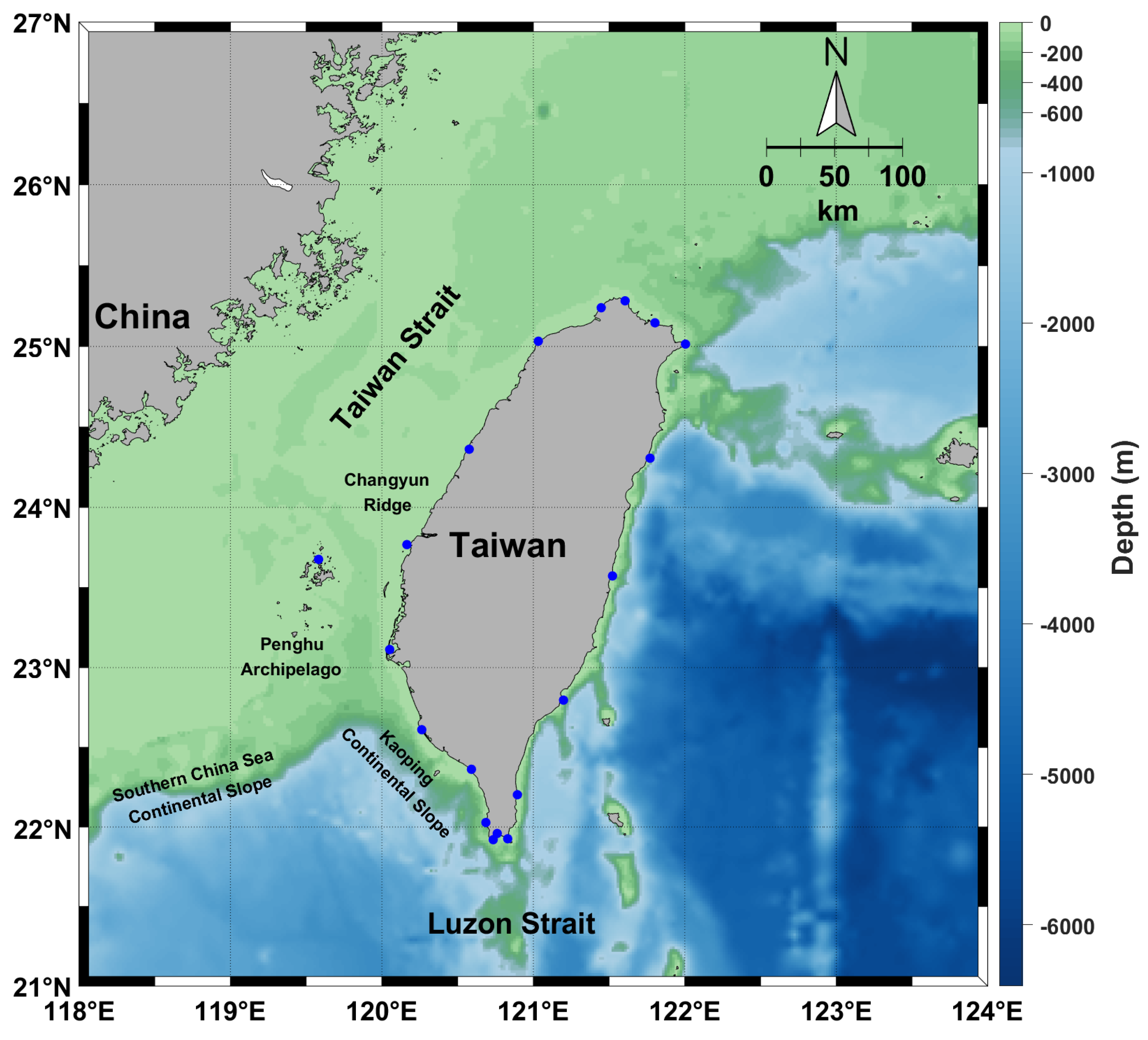
The spatial coverage of the study area is from 21°N to 27°N in latitude and from 118°E to 124°E in longitude as shown in Figure 1. The blue circles show the positions of the CODAR stations. The data covers an area of approximately 195,000 square km. The time span used in this study is from January 2015 to December 2019.
The CODAR data provided by TORI have been preprocessed before delivery to ensure data quality. The data quality control methods described on the website of TORI including (1) the radial velocity data are filtered out if they exceed three times the standard deviation of the data set in the previous month, (2) the percentage of valid data and the output rate exceed 50% within the effective observation radius, and (3) the first-order peak parameters are set according to the statistical results and SeaSonde “Spectral Analysis” is used to reprocess the Doppler spectrum information. The CODAR data after quality control were compared with the current data measured by the drifting buoys. The correlation coefficient increased from 0.754 to 0.962, and the average difference and the root mean square error reduced from 0.007 to 0.000 m/s and from 0.172 to 0.033 m/s, respectively.
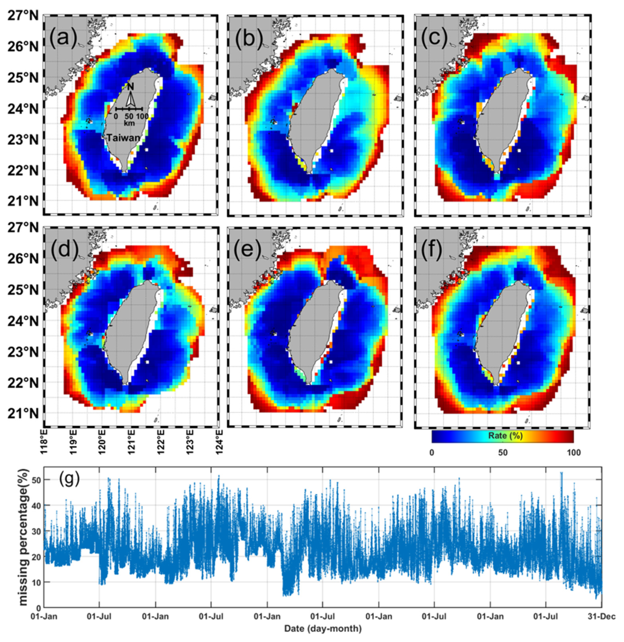
Although CODAR can provide sea surface current data regardless of the weather or time-of-day, Taiwan’s CODAR system does not always provide the data because of maintenance or operation issues. Figure 2 shows the spatial distribution of the missing data rate (Figure 2a–f) and the temporal missing data rate (Figure 2g) from 2015 to 2019. The missing data have to be filled in for later analysis. To fill in the missing data, the Data Interpolating Empirical Orthogonal Function (DINEOF) method [15] was applied in this study. The advantage of DINEOF compared with conventional data filling methods is that it can significantly preserve the physical characteristics of geophysical data. Before performing the DINEOF method, the original data need to be preprocessed into a grid to facilitate subsequent processing. The original data uses hour as a time unit and averages the observation data within each hour to create an hourly sea surface current data file with longitude, latitude, zonal velocity component (positive eastward) and meridional velocity component (positive northward). The spatial resolution was set to 0.1° latitude by 0.1° longitude. The velocity components closest to the centre of each 0.1° grid point were averaged as the representative velocity of the grid point. The grids without the velocity component were set as missing values.
Based on the hourly gridded data, the analysis can be conducted point by point. After deciding the temporal range of the input data and dividing the current velocity into the zonal component U and meridional component V, we can get three-dimensional matrices and respectively. The first to the third dimension of these 3D matrices sequentially stand for the longitude (), latitude (), and time (k). Each element in the matrices means the eastward () or northward () velocity component at the grid point of longitude , latitude , and time of . They can be expressed as:
The next step is to determine the location of the data points. If the kth temporal value at a specific grid point (n, m) is missing, but at least one value of the grid point has data at other times, the grid point is recognized as a data point, and its missing data is reconstructed. Reshaping the zonal and meridional current field matrices after the missing data had been labelled, we convert the matrices into the gridding positions arranged in rows and the recorded times arranged in columns. The new matrices (the zonal component of current velocity), and (the meridional component of current velocity), are two-dimensional arrays in, MN, where M is the grid point (M = 1, 2,, h) and N is the time (N = 1, 2,, k):
After the arrays of and were obtained, they can be combined from top to bottom to generate a 2-D array called X in the form 2M×N [16]:
This data matrix is used for the DINEOF analysis.
DINEOF is a statistical method based on the EOF analysis [17] that can supplement incomplete data and analyze its characteristics. Because the original input data sometimes have missing values, the eigenvalues and eigenvectors are obtained through EOF analysis, and then the estimated values fill in the missing points [18]. The DINEOF method has been widely used to fill in missing data in the geophysical field, such as sea surface temperature or ocean colour images covered by clouds and missing wind or flow field components due to instrument problems. For HF radar data, the occurrence of the missing data may be due to ionosphere clutter, impulsive noise and radio frequency interference [19]. Moreover, the original data provided by TORI have excessive missing data, particularly around the outer boundary of the observation area (see Figure 2). There are many possible reasons for incorrect measurements, such as environmental conditions, antenna placement, measurement range limitations, different types of HF radar (long-range radar or standard radar), and the need for two radars to create a two-dimensional ocean current map with direction and speed. In order to effectively increase the magnitude of the explained variance, the spatial points with a missing data rate greater than 90% are deleted before executing the DINEOF. Later, when applying DINEOF to complement the value, we set the value of the missing points to 0 as an unbiased guess and keep the original values of the points without missing values. With this initial guess, if the actual is 0, these points will be replaced by the reconstructed values, which may or may not be 0. The complete data set is then decomposed using a singular value decomposition (SVD) technique to estimate the spatial and temporal EOFs. The number of retained modes can be changed and adjusted depending on the difference of a diagonal singular value matrix during each iteration [20]. In this study, the sum of explained variances larger than 90% was taken as the iteration number. Further, the convergence was set to a ratio of the root mean square error (RMSE) of missing data to the standard deviation of existing data [20,21] to be less than .
2.3. Cross-Validation
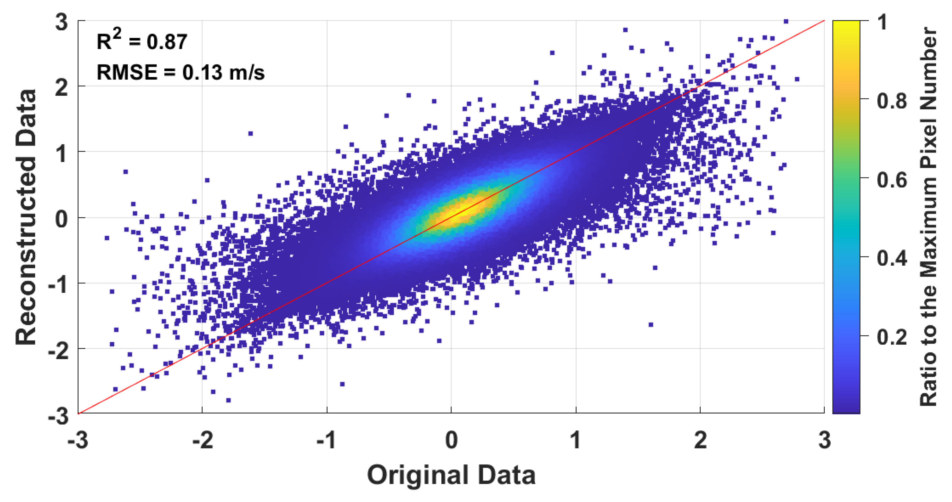
In order to evaluate the accuracy of the reconstructed data, cross-validation was carried out between the original data and the reconstructed data. We randomly selected 1% of the data points from the original images and deleted their values to become missing data as a cross-validation data set [18], and then used the DINEOF method to fill in the missing point values. In the processing of DINEOF analysis iteration, the convergence threshold is set to . The scatter plot of original data and reconstructed data from 2015 to 2019 is shown in Figure 3. The x- and y-axes are the original data and reconstructed data, respectively. The red straight line represents a slope of 1 and an intercept of 0. The ratio of scattering point density is calculated with respect to the maximum data point amount on the position of the coordinate, and the magnitude range of the ratio is between 0 and 1. The colour bar on the right stands for the overlapped level of the data points; the higher data overlapping makes the value tend to 1. The results of the cross-validation show that the coefficient of determination (R2) is 0.87, and the root mean square error (RMSE) is 0.13 m/s.
2.4. EOF Analysis
The EOF analysis is a statistical method to extract the main characteristics of the original data by principal component analysis (PCA), which can present the spatial-temporal variation [17]. It can reduce a data set with a large number of variables to a data set with fewer variables but still retains the main variability of the original data set. By obtaining the eigenvalues and eigenvectors, the spatial patterns and temporal amplitudes (i.e., principal component time-series) of each significant mode are obtained by the SVD technique:
where U is the spatial EOFs, S is the diagonal matrix of singular values (the magnitude of space and time), and V is the temporal EOFs. The spatial patterns of the variance can be represented as P = US. The input data can be expressed as a linear combination of the product of the spatial function and the temporal function as:
where is the spatial patterns of the variance of the ith mode at any given location x, y and is the amplitude of the ith orthogonal mode at time t [22]. As the explained variance decreases with the increasing of mode number, the cumulative variance also grows up to 100%. The number of significant modes can be decided using the estimation [23]:
where is the eigenvalue of the ith principal component, and K is the temporal length of the input data . The error range is presented by a length of the eigenvalue plus and minus the value e as an error bar. When the error range of two principal components overlapped, it means the subsequent components do not have significant physical meaning.
3. Results and Discussion
3.1. Mean State
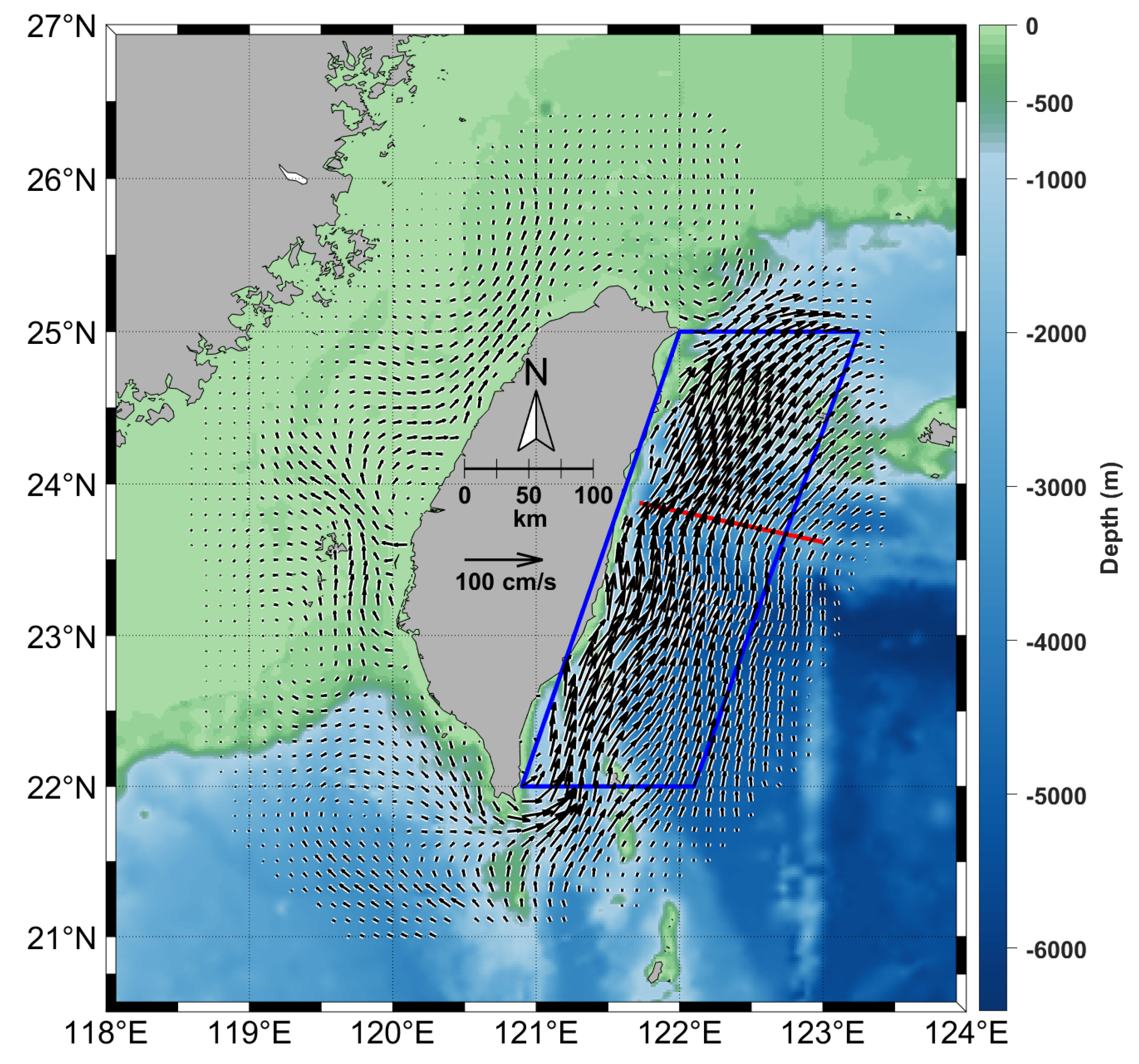
The mean state of the five-year CODAR data is shown in Figure 4. The most obvious feature shows strong northward sea surface currents off the east coast of Taiwan Island; this is the Kuroshio. In the Taiwan Strait, the sea surface currents are relatively weak compared with that of the Kuroshio. The average sea surface current speed in the Kuroshio region is 0.62 m/s, 0.71 m/s in summer, and 0.55 m/s in winter. In the Taiwan Strait, it is 0.29 m/s on average, 0.32 m/s in summer, and 0.28 m/s in winter. The sea surface currents in the Taiwan Strait generally flow northward but are affected by the topography. For example, when the sea surface currents approach the Changyun Ridge (see Figure 1), they turn to the northwest and then turn back to the north after passing it. The sea surface currents also turn to the southeast when they encounter the Kaoping Continental Slope (see Figure 1). In order to verify the CODAR data, it was compared with the in-situ measurements of the KTV1 line in the Kuroshio region. The average maximum sea surface current velocity of CODAR along the KTV1 line is 0.9 m/s using reconstructed data and 0.93 m/s using the original data. The value is almost the same as the climatological maximum current speed of 0.90 m/s along the KTV1 line [24].
3.2. EOF Results
3.2.1. Entire Study Area
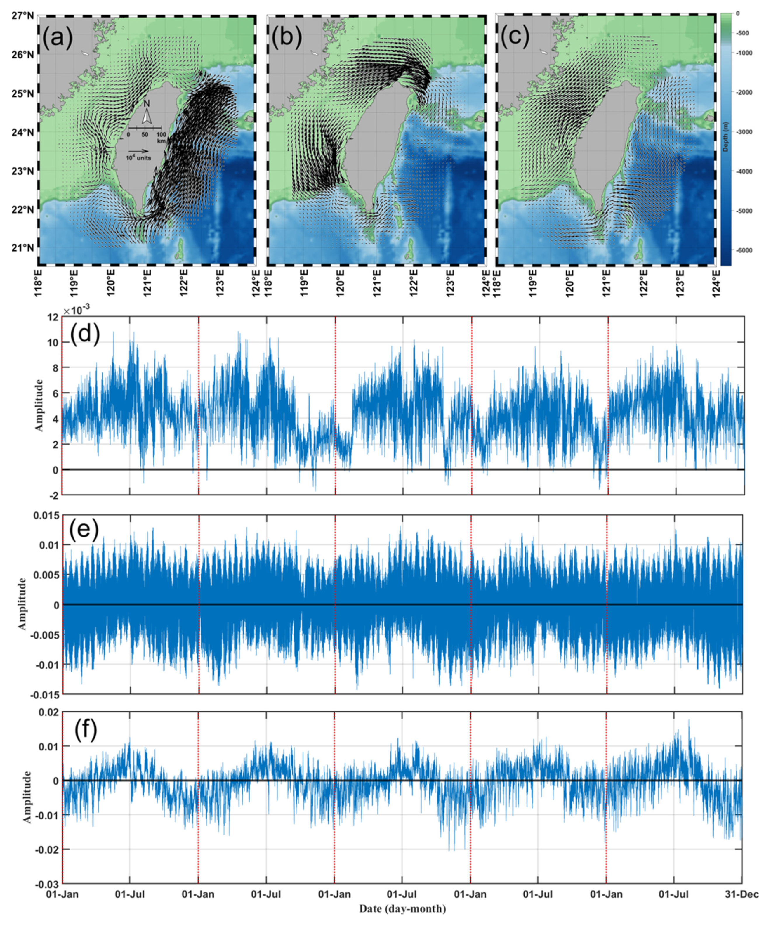
The first three EOF modes for the five-year data in the entire study area are shown in Figure 5. The first EOF mode (EOF1) accounts for 24% of the total variance. The spatial pattern is similar to the mean state. This shows that there are strong sea surface currents east of Taiwan Island. The corresponding principal components of the time series are almost all positive, implying that the flow field is dominated by northward flow, i.e., the Kuroshio. The amplitude and amplitude variation of principal components are larger in summer than that in winter, implying that the Kuroshio is stronger in summer and its variation is also larger. In the Taiwan Strait, most of the currents are northward and modulated by the topography. One can see that the Changyun Ridge (See Figure 1) located in the middle strait partially obstructs the northward currents along the western coast of Taiwan Island, forces them to turn west and then turn back after passing the ridge. In addition, parts of the northward currents along the South China Sea Continental Slope and Kaoping Continental Slope turn to the Luzon Strait.
The second EOF mode (EOF2) accounts for 11% of the total variance. It shows strong sea surface currents in the northern and southern Taiwan Strait and relatively weak in the Kuroshio region. From the time series of principal components, one can see that the frequency is mainly tide-dominant, implying that EOF2 displays the tidal currents in the study area. Strong tidal currents are presented around the Penghu Archipelago and the northern tip of Taiwan Island but are very weak in the Kuroshio region.
The third EOF mode (EOF3) accounts for 5% of the total variance. The time series of principal components show positive values in winter and negative values in summer. This seasonal current direction reversal may be caused by the monsoon winds. The spatial pattern shows strong sea surface currents in the northern Taiwan Strait. This may be due to the shallow and narrow topography there.
To understand the characteristics of sea surface currents in more detail, the study area is further divided into the Kuroshio region east of Taiwan Island and the Taiwan Strait area west of Taiwan Island, and EOF analysis is carried out year by year from 2015 to 2019.
3.2.2. Kuroshio Region
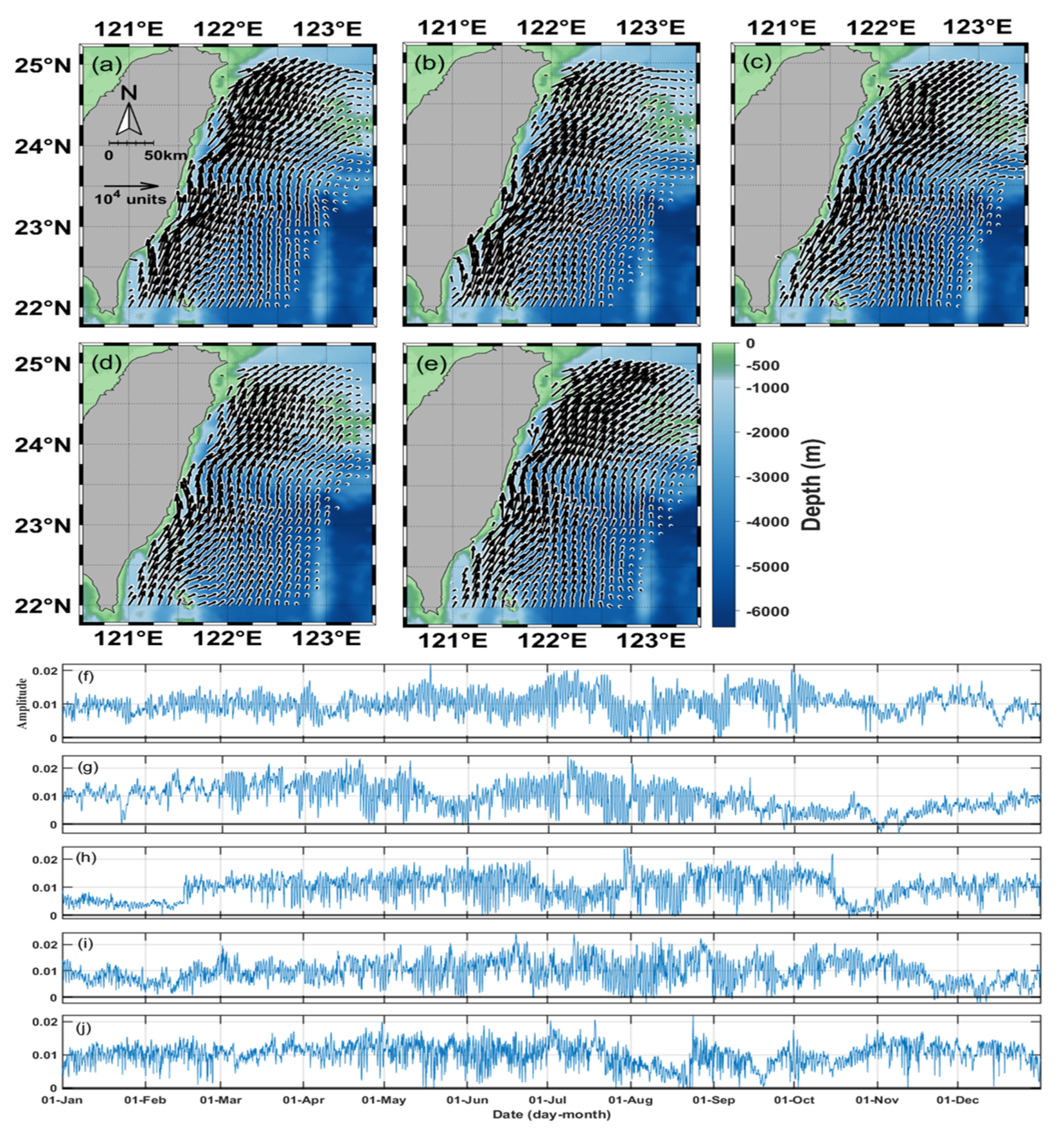
The yearly EOF1 modes of the Kuroshio area are shown in Figure 6. The explained variance values are 58.21%, 52.25%, 52.50%, 44.72%, and 55.17% from 2015 to 2019, respectively. The principal components show that almost all values are positive. This mode can represent the general state of the Kuroshio. The spatial pattern shows strong currents near the east coast of Taiwan Island, which is the core area of the Kuroshio. From the time series of principal components, one can see that the variation is greater in summer (June, July, and August) than in winter (December, January, and February). The root-mean-square (RMS) method is used to represent the variation [25]. Table 1 shows the variation of principal components in each year from 2015 to 2019. The range of variations was between 4.05 × 10⁻³ and 4.99 × 10⁻³, which is 1–2 times the range of variation in winter between 2.29 × 10⁻³ and 3.08 × 10⁻³. Combining the spatial values and the corresponding principal components, the sea surface velocities in the Kuroshio region can be calculated. From 2015 to 2019, the average sea surface current velocity in the Kuroshio core area ranged from 0.60 to 0.64 m/s in summer and 0.47 to 0.58 m/s in winter. The Kuroshio velocity is larger in summer than in winter. Table 2 shows the average sea surface velocity, maximum sea surface velocity, and variation in summer and winter from 2015 to 2019. Regardless of the maximum velocity, average velocity, or velocity, the variation in summer is greater than in winter.
Previous studies [26,27] have used satellite altimetry and in-situ measurements to report that the Kuroshio intensifies in summer and weakens in the winter. This study yields similar results but provided more detailed information about the seasonal variations of the Kuroshio. Note that these values of sea surface current velocities represent only the Kuroshio itself and do not include the effects of eddies and others, such as typhoons.
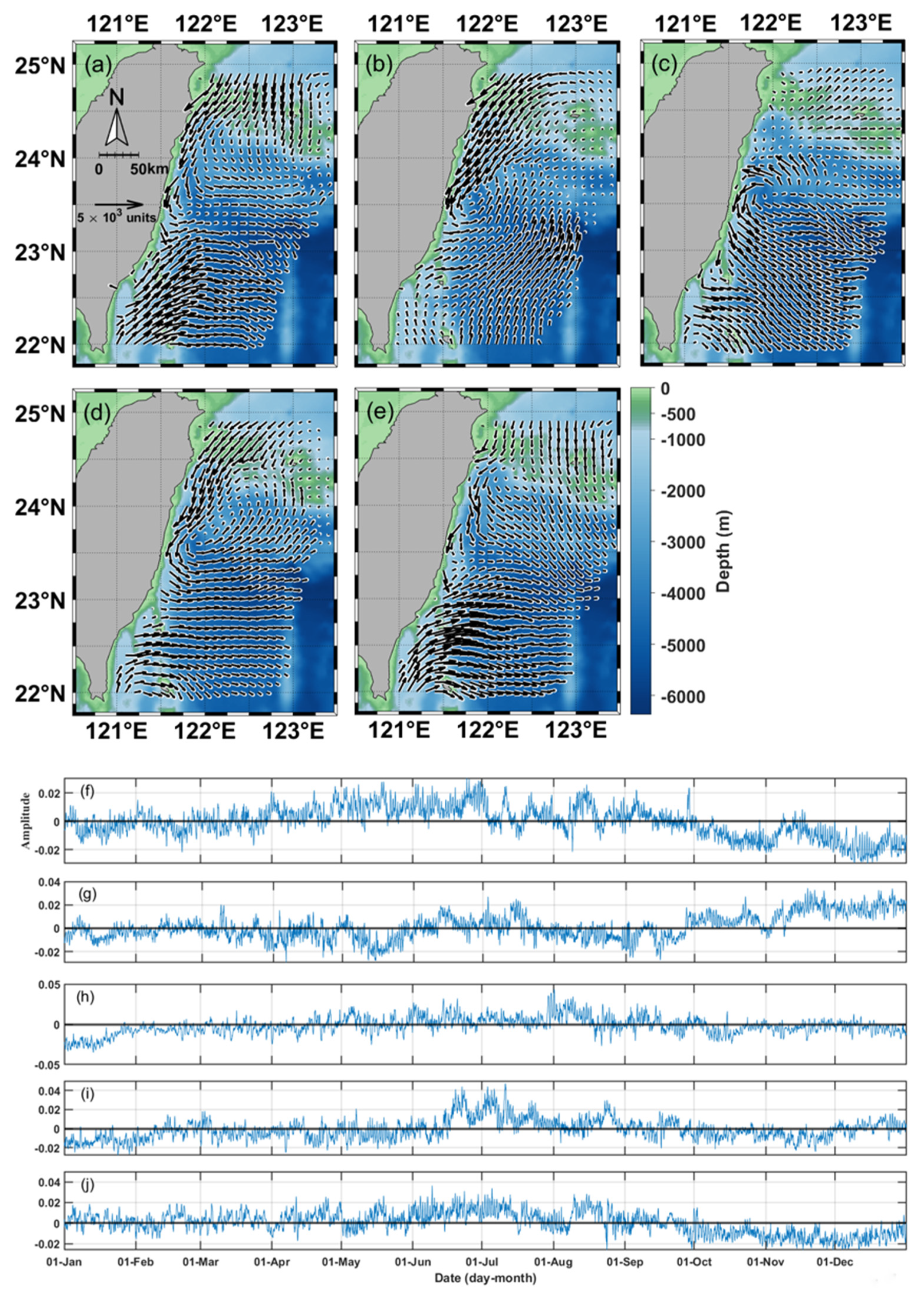
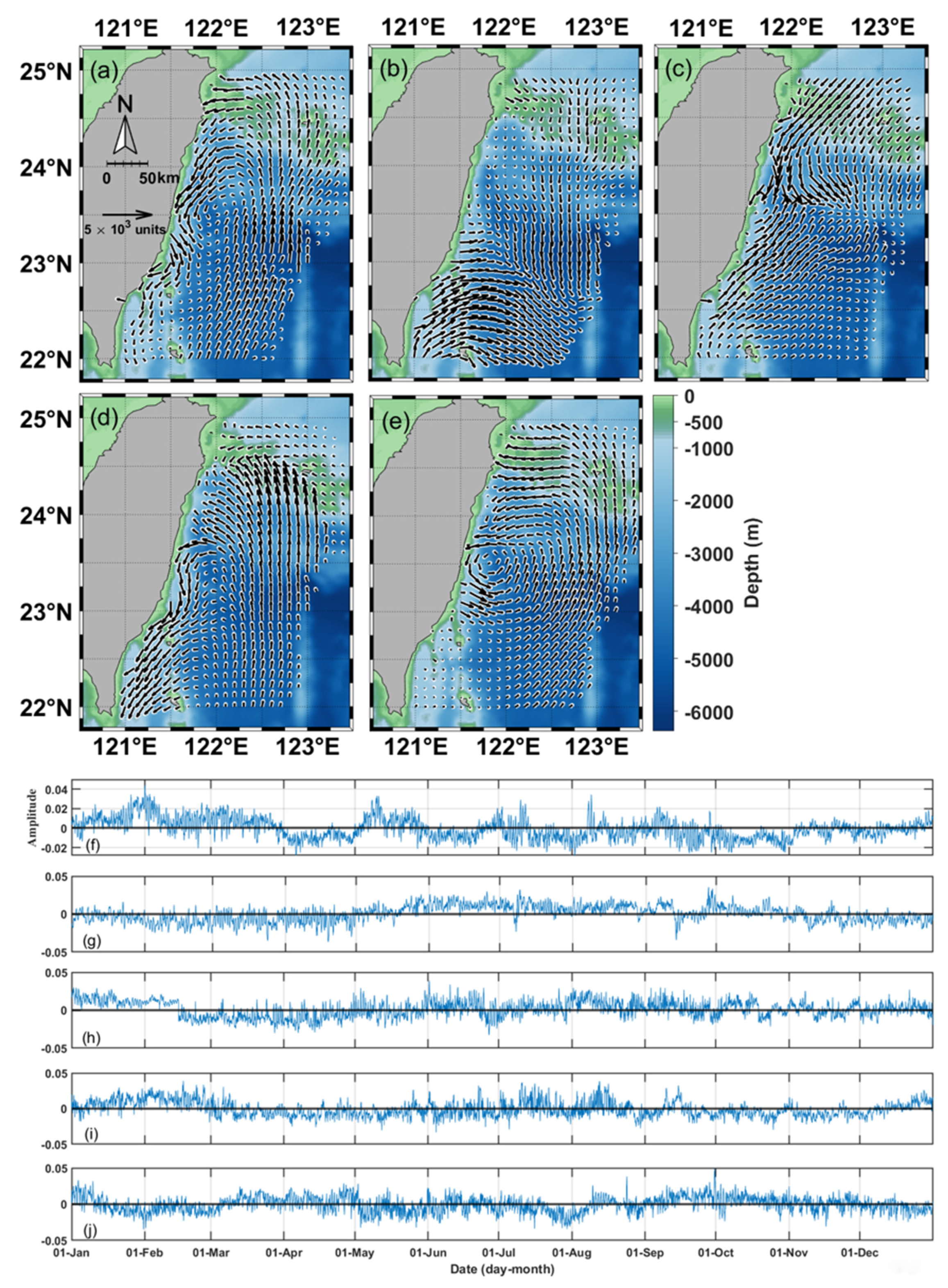
The yearly EOF2 modes are shown in Figure 7. The explained variances are 5.81%, 4.72%, 4.25%, 5.29%, and 6.02% from 2015 to 2019, respectively. The spatial pattern showed that there was a dipole eddy pair in 2015, 2018, and 2019 and a signal eddy in 2016 and 2017. A similar phenomenon is presented in the EOF3, as shown in Figure 8. There was a signal eddy in 2015, 2018, and 2019 and a dipole eddy pair in 2016 and 2017. The explained variances of EOF3 are 2.87%, 3.86%, 3.18%, 4.09% and 2.47% from 2015 to 2019, respectively. The previous study [4] has presented that dipole eddy pair and/or single eddy from the western North Pacific impinge(s) on the Kuroshio and affect(s) the Kuroshio velocity and transport. From spatial patterns of EOF2 in 2015, 2018 and 2019, one can see that the cyclonic (anticyclonic) eddy was located in the north (south) of the eddy pair, respectively. The corresponding principal components show that most values are positive in summer and negative in winter. Combined with the spatial distribution, this means that in summer, the cyclonic (anticyclonic) eddies are located on the north (south) side more frequently. This may create cross-stream flow divergence, thereby reducing the Kuroshio downstream transport. In contrast, the reversal cases, i.e., the cyclonic eddy on the south side and the anticyclonic eddy on the north side occur mostly in winter. This may form cross-stream flow convergence, thereby increase the Kuroshio downstream transport.
From the spatial patterns of EOF2 in 2016 and 2017 and EOF3 in 2015, 2018, and 2019, one can see a single eddy located at around 23°N, 122°E. Combined with the corresponding principal component, a cyclonic (an anticyclonic) eddy corresponds to a positive (negative) value. If a cyclonic (an anticyclonic) eddy approaches the Kuroshio off eastern Taiwan, it will decrease (increase) the Kuroshio northward velocity and transport [28]. Nevertheless, it is difficult to find obvious exchange regularity between the positive and negative values of the corresponding principal components. Previous studies have mentioned that eddies approaching the Kuroshio region east of Taiwan Island affected the Kuroshio at different periods, e.g., 30–70 days [29,30] and 100–200 days [4,30,31]. The above-mentioned results indicate that the various periods of the Kuroshio range from 30 to 200 days.
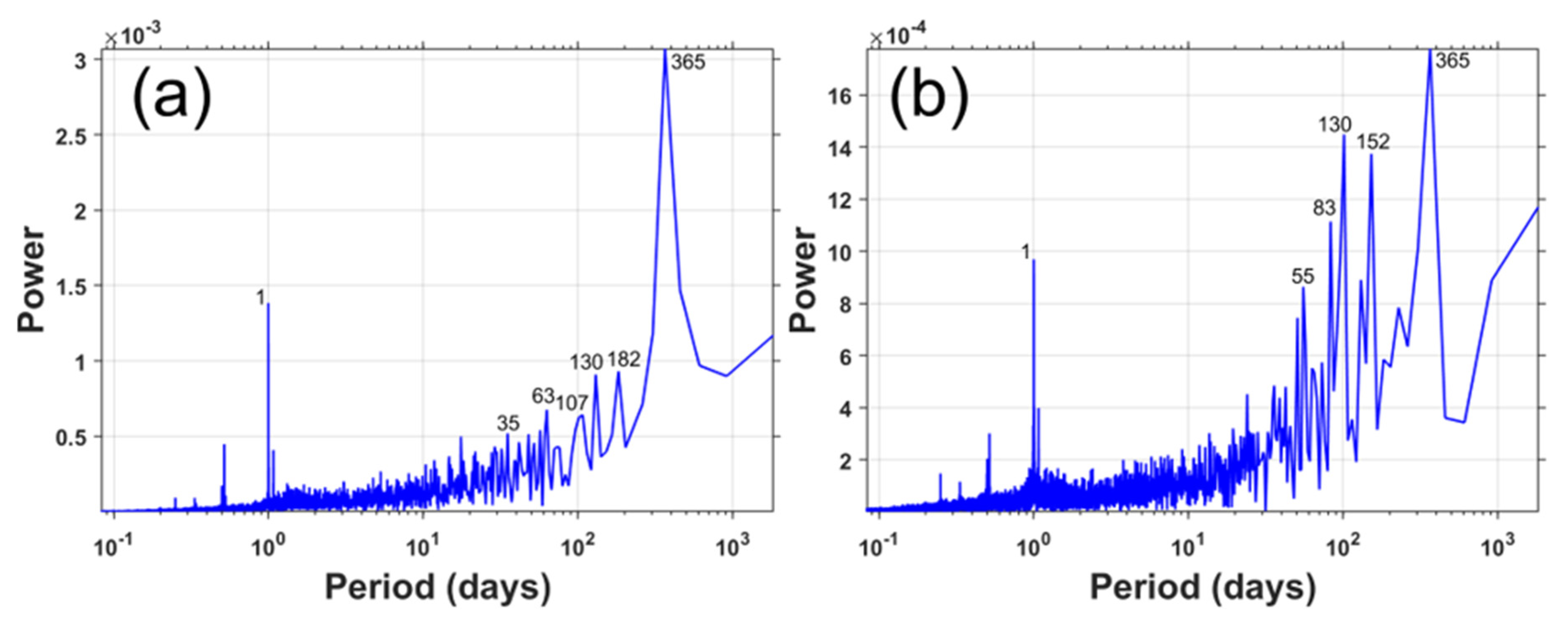
In order to examine the various periods of the dipole eddy pair and the single eddy, the 5-year data in the Kuroshio region were analyzed by the EOF analysis and the power spectrum of corresponding time series by the Fast Fourier Transform (FFT). The EOF results show that the dipole eddy pair pattern in EOF2 (4.68% of total variance) and the single eddy pattern in EOF3 (2.97% of total variance) as shown in Figure 9. The power spectra of both principal components are shown in Figure 10. One can see that the dominant periods of the dipole eddy pair are the daily and annual cycles, although there are some periods of small power peaks at 35, 63, 107, 130, and 182 days. For the single eddy, there are multiple periods; in addition to the daily and annual cycles, there are 55, 83, 101, and 152 days.
3.2.3. Taiwan Strait
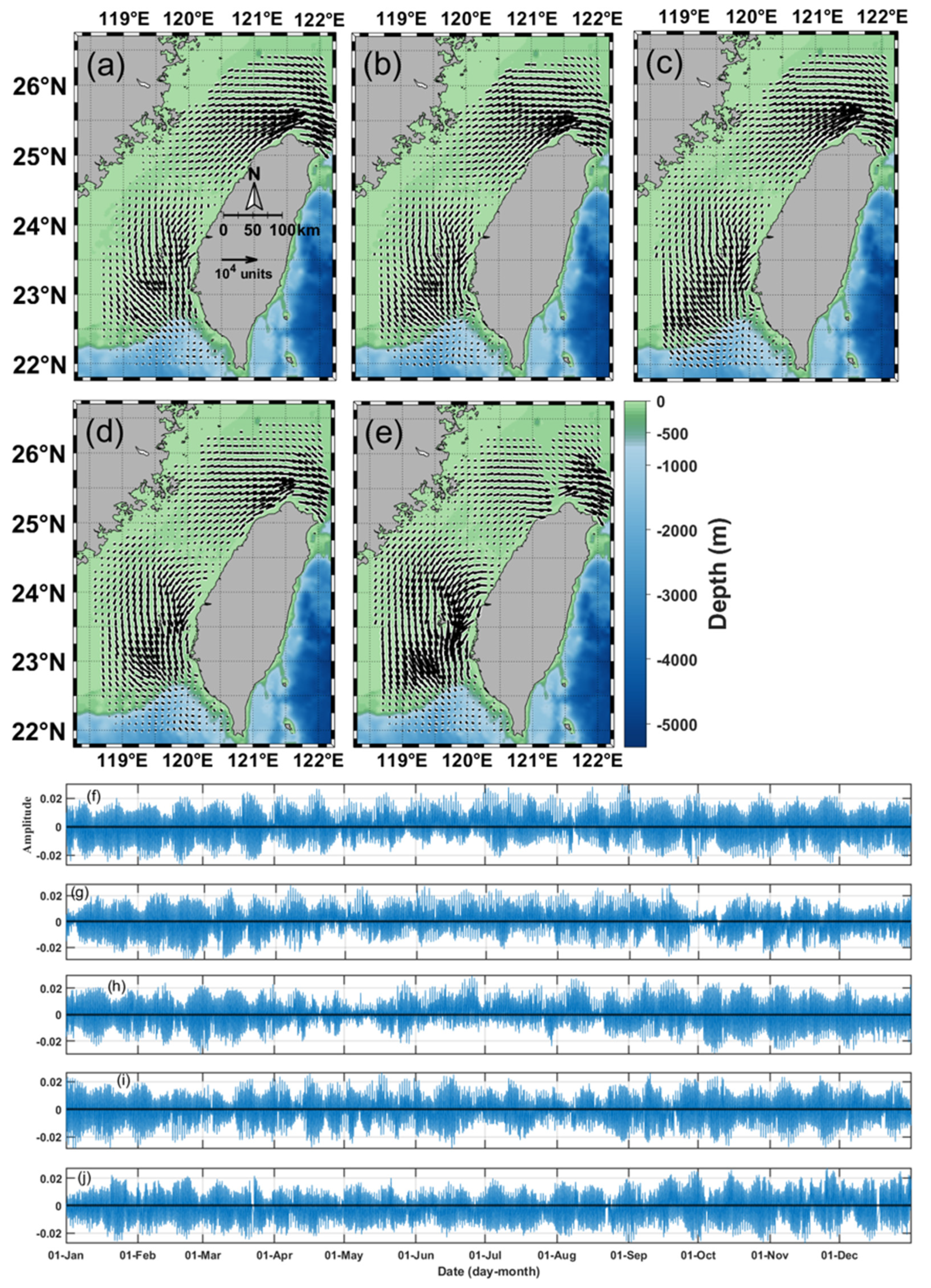
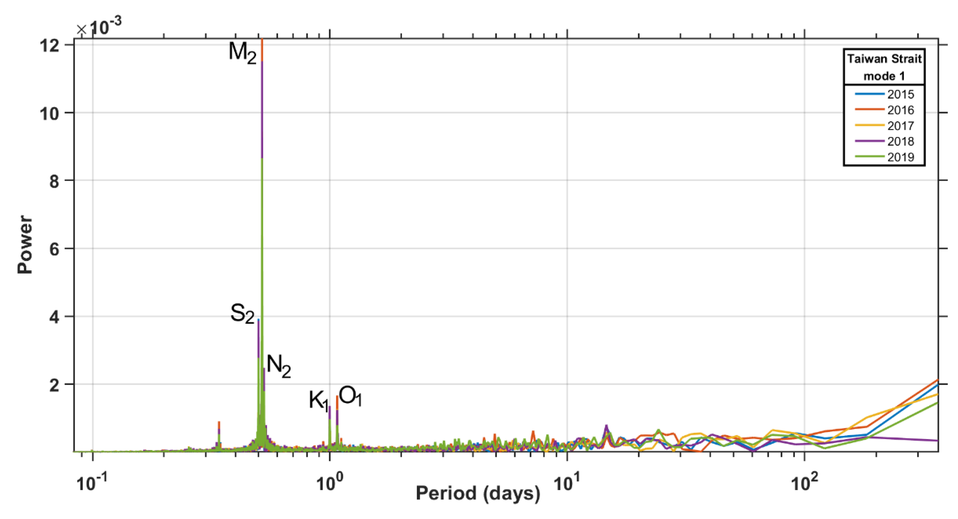
The EOF analysis of the currents in the Taiwan Strait is only statistically significant in the first and second modes. The EOF1 modes show that the explained variances were 33.37%, 28.82%, 29.58%, 26.56%, and 32.02% from 2015 to 2019, respectively. The time series of the principal components seem to be of the tidal periods (Figure 11). Performing the FFT analysis on the time series of the principal components year by year yields the most significant period was 12.42 hours, which corresponds to the M2 semi-diurnal tide period as shown in Figure 12. In addition to the M2 tide, the other two peaks can also be found at 12.00 hours and 12.66 hours, corresponding to the S2 and N2 semi-diurnal tide periods, respectively. There are two smaller peaks near the daily period, 23.93 hours and 25.76 hours, belonging to the diurnal tide of K1 and O1, respectively. The tide enters the Taiwan Strait from the north and south of the Taiwan Strait. The spatial patterns from 2015 to 2018 show the formation of strong tidal currents around the northern tip of Taiwan Island and the Penghu Archipelago. The results are similar to the positions of faster elliptical tidal currents in the Taiwan Strait, as shown in the work [6]. However, the spatial pattern in 2019 did not show the same strong tidal currents at the northern tip of Taiwan Island. This may be due to a large number of missing values in the CODAR data in that year (see Figure 2). Although the DINEOF method is used to fill the missing data in this study, the grid points with a missing data rate exceeding 90% are eliminated. As a result, the tidal currents in this area become smaller in 2019.
The sea surface current velocity of the tidal component can be calculated by combining the spatial and temporal values of the EOF1 modes. Table 3 shows the occurrence time and velocity of the maximum tidal current from 2015 to 2019 near the northern tip of the Taiwan Island and around the Penghu Archipelago. They almost all occurred during the spring tide, except in 2019. The maximum tidal current velocity occurred in 2017. These values are relatively stable except for the values in 2019. This is probably because of the long-term lack of data near the northern tip of Taiwan Island that year. The previous study [8] used a harmonic analysis on the measured surface currents from two Ocean State Monitoring and Analyzing Radars (OSMAR) in a small proportion of the Taiwan Strait near the coast of Fujian, China. Its results showed that the M2 tidal constituent is dominant in that study area. In this study, not only the M2 tide but also other major tidal constituents were observed.
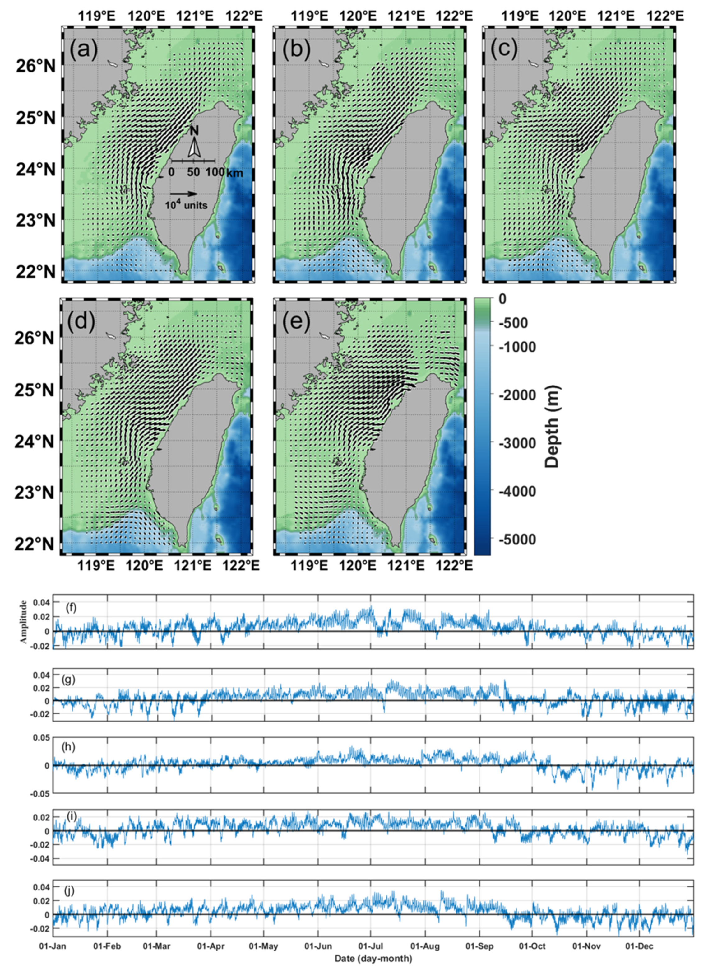
The explained variances of EOF2 modes are 14.24%, 16.06%, 12.98%, 15.40%, and 15.34% from 2015 to 2019, respectively. One can see a seasonal signal on its corresponding principal components, with the most positive values in summer and negative values in winter, as shown in Figure 13. Combined with the spatial patterns, it clearly shows that the current directions in the Taiwan Strait are northward in summer while reversing southward in winter. This current direction reversal is mainly controlled by the monsoon winds, i.e., the southwesterly winds prevail in summer and the northeasterly winds in winter. It is found from the spatial distribution that the sea surface currents in the northern Taiwan Strait are relatively strong due to its narrowing horizontal width and shoaling bottom topography. The maximum five-year average velocity reaches 1.22 m/s northward in summer and the same velocity but southward in winter.
4. Summary
This study aims to analyze the sea surface currents around Taiwan Island, using hourly CODAR current data and the EOF analysis method. The high spatiotemporal resolution data set provides more details and comprehensive characteristics of the sea surface circulation. Before performing the EOF analysis, the DINEOF method was applied to fill in the missing CODAR data to obtain a complete data set. The results reveal the major characteristics of the sea surface currents around Taiwan Island, which are summarized as follows.
- The Kuroshio surface currents have remarkable seasonal variation. In summer, it is stronger with a mean current velocity as high as 0.62 m/s and a larger variation of 0.19 m/s. In winter, the mean current velocity decreases to 0.54 m/s and a variation of 0.14 m/s. It has to be noted that these values of sea surface current velocities are only the Kuroshio itself and do not include the effects of eddies or others.
- It is a frequently occurring phenomenon that the dipole eddy pairs impinge on the Kuroshio. In most cases, the cyclonic/anticyclonic eddy occurs on the north/south side in summer, and the polarity reverses in winter. These characteristics result in the Kuroshio downstream transport decreasing in summer and increasing in winter.
- The single eddy impinging on the Kuroshio occurs at different periods, including daily, intraseasonal (55 and 83 days), interseasonal (101 and 152 days), and annual periods.
- The tidal currents are dominant components of the surface circulation in the Taiwan Strait. The maximum tidal current velocity reaches as high as 1.75 m/s around the northern tip of Taiwan Island and 1.50 m/s around the Penghu Archipelago.
- The monsoon winds are an important driven forcing for sea surface currents in the Taiwan Strait, which are characterized by strong currents as high as 1.22 m/s in the northern strait due to the narrowing and shoaling topography.
Author Contributions
Conceptualization, C.-R.H.; methodology, C.-R.H. and Y.-H.T.; software, Y.-H.T. and C.-Y.L.; validation, Y.-H.T. and C.-Y.L.; writing-original draft preparation, C.-R.H. and Y.-H.T.; writing-review and editing: Q.Z. and C.-R.H.; funding acquisition: C.-R.H. All authors have read and agreed to the published version of the manuscript.
Funding
This research was funded by the Ministry of Science and Technology of Taiwan, Grant MOST 109-2811-M-019-011 and the Central Weather Bureau of Taiwan Grant 1102084A.
Institutional Review Board Statement
Not applicable.
Informed Consent Statement
Not applicable.
Data Availability Statement
The data presented in this study are available on request from the corresponding author. The data are not publicly available due to they cannot be used for free.
Acknowledgments
The authors appreciate TORI for providing CODAR data and permission for publication.
Conflicts of Interest
The authors declare no conflict of interest.
References
- Lien, R.C.; Ma, B.; Cheng, Y.H.; Ho, C.R.; Qiu, B.; Lee, C.M.; Chang, M.H. Modulation of Kuroshio transport by mesoscale eddies at the Luzon Strait entrance. J. Geophys. Res. Oceans 2014, 119, 2129–2142. [Google Scholar] [CrossRef]
- Tsai, C.J.; Andres, M.; Jan, S.; Mensah, V.; Sanford, T.B.; Lien, R.C.; Lee, C.M. Eddy-Kuroshio interaction processes revealed by mooring observations off Taiwan and Luzon. Geophys. Res. Lett. 2015, 42, 8098–8105. [Google Scholar] [CrossRef] [Green Version]
- Cheng, Y.H.; Ho, C.R.; Zheng, Q.; Qiu, B.; Hu, J.; Kuo, N.-J. Statistical features of eddies approaching the Kuroshio east of Taiwan Island and Luzon Island. J. Oceanogr. 2017, 73, 427–438. [Google Scholar] [CrossRef]
- Chang, M.H.; Jan, S.; Mensah, V.; Andres, M.; Rainville, L.; Yang, Y.J.; Cheng, Y.H. Zonal migration and transport variations of the Kuroshio east of Taiwan induced by eddy impingements. Deep-Sea Res. PT I 2018, 131, 1–15. [Google Scholar] [CrossRef]
- Zheng, Q.; Ho, C.R.; Xie, L.; Li, M. A case study of a Kuroshio main path cut-off event and impacts on the South China Sea in fall-winter 2013-2014. Acta Oceanol. Sin. 2019, 38, 12–19. [Google Scholar] [CrossRef]
- Jan, S.; Wang, Y.H.; Chao, S.Y.; Wang, D.P. Development of a nowcast system for the Taiwan Strait (TSNOW): Numerical simulation of barotropic tides. Ocean. Polar Res. 2001, 23, 195–203. [Google Scholar]
- Chuang, W.S. A note on the driving mechanisms of current in the Taiwan Strait. J. Oceanogr. 1986, 42, 355–361. [Google Scholar] [CrossRef]
- Lai, Y.; Zhou, H.; Wen, B. Surface current characteristics in the Taiwan Strait observed by high-frequency radars. IEEE J. Ocean. Eng. 2016, 42, 449–457. [Google Scholar] [CrossRef]
- Lipa, B.; Barrick, D.; Isaacson, J. Evaluating hf coastal radar site performance for tsunami warning. Remote Sens. 2019, 11, 2773. [Google Scholar] [CrossRef] [Green Version]
- Roarty, H.; Cook, T.; Hazard, L.; George, D.; Harlan, J.; Cosoli, S.; Wyatt, L.; Alvarez, F.E.; Terrill, E.; Otero, M.; et al. The global high frequency radar network. Front. Mar. Sci. 2019, 6, 164. [Google Scholar] [CrossRef]
- Fujii, S.; Heron, M.L.; Kim, K.; Lai, J.W.; Lee, S.H.; Wu, X.; Wu, X.; Wyatt, L.R.; Yang, W.C. An overview of developments and applications of oceanographic radar networks in Asia and Oceania countries. Ocean. Sci. J. 2013, 48, 69–97. [Google Scholar] [CrossRef]
- Crombie, D.D. Doppler spectrum of sea echo at 13.56 Mc./s. Nature 1955, 175, 681–682. [Google Scholar] [CrossRef]
- Barrick, D.E.; Evans, M.W.; Weber, B.L. Ocean surface currents mapped by radar. Science 1977, 198, 138–144. [Google Scholar] [CrossRef]
- Paduan, J.D.; Washburn, L. High-frequency radar observations of ocean surface currents. Annu. Rev. Mar. Sci. 2013, 5, 115–136. [Google Scholar] [CrossRef] [Green Version]
- Beckers, J.M.; Rixen, M. EOF Calculations and Data Filling from Incomplete Oceanographic Datasets. J. Atmos. Ocean. Technol. 2003, 20, 1839–1856. [Google Scholar] [CrossRef]
- Kuo, N.J. Satellite observation of the cold water around the Hainan Island. In Satellite Remote Sensing of South China Sea; Liu, A.K., Ho, C.R., Liu, C.T., Eds.; Tingmao Publish Company: Taiwan, 2008; pp. 159–170. [Google Scholar]
- Thomson, R.E.; Emery, W.J. Data Analysis Methods in Physical Oceanography, 3rd ed.; Elsevier: Boston, MA, USA, 2014; ISBN 978-0-12-387782-6. [Google Scholar]
- Alvera-Azcárate, A.; Barth, A.; Sirjacobs, D.; Lenartz, F.; Beckers, J.M. Data Interpolating Empirical Orthogonal Functions (DINEOF): A tool for geophysical data analyses. Mediterr. Mar. Sci. 2011, 12, 5–11. [Google Scholar] [CrossRef] [Green Version]
- Nazari, M.E.; Huang, W.; Zhao, C. Radio frequency interference suppression for HF surface wave radar using CEMD and temporal windowing methods. IEEE Geosci. Remote Sens. Lett. 2019, 17, 212–216. [Google Scholar] [CrossRef]
- Huynh, H.N.T.; Alvera-Azcárate, A.; Barth, A.; Beckers, J.M. Reconstruction and analysis of long-term satellite-derived sea surface temperature for the South China Sea. J. Oceanogr. 2016, 72, 707–726. [Google Scholar] [CrossRef]
- Ping, B.; Su, F.; Meng, Y. An improved DINEOF algorithm for filling missing values in spatio-temporal sea surface temperature data. PLoS ONE 2016, 11, e0155928. [Google Scholar] [CrossRef] [Green Version]
- Kuo, N.J.; Ho, C.R. ENSO effect on the sea surface wind and sea surface temperature in the Taiwan Strait. Geophys. Res. Lett. 2004, 31, L13309. [Google Scholar] [CrossRef]
- North, G.R.; Bell, T.L.; Cahalan, R.F.; Moeng, F.J. Sampling errors in the estimation of empirical orthogonal functions. Mon. Weather Rev. 1982, 110, 699–706. [Google Scholar] [CrossRef]
- Jan, S.; Yang, Y.J.; Wang, J.; Mensah, V.; Kuo, T.H.; Chiou, M.D.; Chern, C.S.; Chang, M.H.; Chien, H. Large variability of the Kuroshio at 23.75 N east of Taiwan. J. Geophys. Res. Oceans 2015, 120, 1825–1840. [Google Scholar] [CrossRef]
- Ho, C.R.; Kuo, N.J.; Zheng, Q.; Soong, Y.S. Dynamically active areas in the South China Sea detected from TOPEX/POSEIDON satellite altimeter data. Remote Sens. Environ. 2000, 71, 320–328. [Google Scholar] [CrossRef]
- Hsin, Y.C.; Qiu, B.; Chiang, T.L.; Wu, C.R. Seasonal to interannual variations in the intensity and central position of the surface Kuroshio east of Taiwan. J. Geophys. Res. Oceans 2013, 118, 4305–4316. [Google Scholar] [CrossRef]
- Lee, T.N.; Johns, W.E.; Liu, C.T.; Zhang, D.; Zantopp, R.; Yang, Y. Mean transport and seasonal cycle of the Kuroshio east of Taiwan with comparison to the Florida Current. J. Geophys. Res. Oceans 2001, 106, 22143–22158. [Google Scholar] [CrossRef] [Green Version]
- Kuo, Y.C.; Chern, C.S. Numerical study on the interactions between a mesoscale eddy and a western boundary current. J. Oceanogr. 2011, 67, 263–272. [Google Scholar] [CrossRef]
- Hsin, Y.C.; Wu, C.R.; Shaw, P.T. Spatial and temporal variations of the Kuroshio east of Taiwan, 1982–2005: A numerical study. J. Geophys. Res. Oceans 2008, 113, C04002. [Google Scholar] [CrossRef] [Green Version]
- Hsu, P.C.; Lin, C.C.; Huang, S.J.; Ho, C.R. Effects of cold eddy on Kuroshio meander and its surface properties, east of Taiwan. IEEE J. Sel. Top. Appl. Earth Obs. Remote Sens. 2016, 9, 5055–5063. [Google Scholar] [CrossRef]
- Qiu, B.; Chen, S. Interannual variability of the North Pacific Subtropical Countercurrent and its associated mesoscale eddy field. J. Phys. Oceanogr. 2010, 40, 213–225. [Google Scholar] [CrossRef]
Figure 1.
The study area and locations of Taiwan’s CODAR system (blue dots).

Figure 2.
The spatial missing data rate in year of (a) 2015, (b) 2016, (c) 2017, (d) 2018, (e) 2019, and (f) 2015–2019, and (g) the temporal missing data rate in 2015–2019.
Figure 2.
The spatial missing data rate in year of (a) 2015, (b) 2016, (c) 2017, (d) 2018, (e) 2019, and (f) 2015–2019, and (g) the temporal missing data rate in 2015–2019.

Figure 3.
A scatter plot of the 1% missing data between original data and reconstructed data. The red line is the alignment. The colour bar stands for the overlapped level of the data points.
Figure 3.
A scatter plot of the 1% missing data between original data and reconstructed data. The red line is the alignment. The colour bar stands for the overlapped level of the data points.

Figure 4.
Mean current field of reconstructed data and the KTV1 line (red line). The blue parallelogram stands for the area of core current.
Figure 4.
Mean current field of reconstructed data and the KTV1 line (red line). The blue parallelogram stands for the area of core current.

Figure 5.
The spatial distribution of the EOF results, (a) the first EOF mode (EOF1), (b) the second EOF mode (EOF2) and (c) the third EOF mode (EOF3) of five-year data in the whole area around Taiwan and the corresponding time series of principal components, (d) EOF1, (e) EOF2 and (f) EOF3.
Figure 5.
The spatial distribution of the EOF results, (a) the first EOF mode (EOF1), (b) the second EOF mode (EOF2) and (c) the third EOF mode (EOF3) of five-year data in the whole area around Taiwan and the corresponding time series of principal components, (d) EOF1, (e) EOF2 and (f) EOF3.

Figure 6.
The EOF1 of Kuroshio region. (a–e) The spatial modes from 2015 to 2019. (f–j) The time series of principal components from 2015 to 2019.
Figure 6.
The EOF1 of Kuroshio region. (a–e) The spatial modes from 2015 to 2019. (f–j) The time series of principal components from 2015 to 2019.

Figure 7.
Same as Figure 6, but for EOF2.
Figure 7.
Same as Figure 6, but for EOF2.

Figure 8.
Same as Figure 6, but for EOF3.
Figure 8.
Same as Figure 6, but for EOF3.

Figure 9.
EOF results of 5-year data. Spatial pattern of (a) mode 2, (b) mode 3, and corresponding time series of principal components of (c) mode 2, (d) mode 3.
Figure 9.
EOF results of 5-year data. Spatial pattern of (a) mode 2, (b) mode 3, and corresponding time series of principal components of (c) mode 2, (d) mode 3.


Figure 11.
EOF1 results of the Taiwan Strait.

Figure 12.
Power spectra of EOF1 principal components of the Taiwan Strait.

Figure 13.
Same as Figure 11, but for EOF2.
Figure 13.
Same as Figure 11, but for EOF2.


Table 1.
Variations of EOF1 principal components.
| Year | Summer (×10−3) | Winter (×10−3) | Ratio (Summer/Winter) |
|---|---|---|---|
| 2015 | 4.20 | 2.29 | 1.83 |
| 2016 | 4.89 | 3.08 | 1.59 |
| 2017 | 4.76 | 3.54 | 1.34 |
| 2018 | 4.99 | 2.95 | 1.69 |
| 2019 | 4.05 | 2.46 | 1.65 |
Table 2.
Average sea surface velocity, maximum sea surface velocity, and variation in summer and winter (unit: m/s).
Table 2.
Average sea surface velocity, maximum sea surface velocity, and variation in summer and winter (unit: m/s).
| Average Velocity | Maximum Velocity | Velocity Variation | |||||||
|---|---|---|---|---|---|---|---|---|---|
| Year | Summer | Winter | Ratio (Summer/Winter) | Summer | Winter | Ratio (Summer/Winter) | Summer | Winter | Ratio (Summer/Winter) |
| 2015 | 0.64 | 0.55 | 1.16 | 1.44 | 1.20 | 1.20 | 0.20 | 0.14 | 1.43 |
| 2016 | 0.62 | 0.55 | 1.13 | 1.75 | 1.43 | 1.22 | 0.20 | 0.16 | 1.25 |
| 2017 | 0.62 | 0.54 | 1.15 | 1.75 | 1.11 | 1.58 | 0.20 | 0.14 | 1.43 |
| 2018 | 0.60 | 0.47 | 1.28 | 1.46 | 0.95 | 1.54 | 0.18 | 0.10 | 1.80 |
| 2019 | 0.61 | 0.58 | 1.05 | 1.63 | 1.19 | 1.37 | 0.19 | 0.15 | 1.27 |
| mean | 0.62 | 0.54 | 1.15 | 1.61 | 1.18 | 1.38 | 0.19 | 0.14 | 1.43 |
Table 3.
The maximum tidal velocity during the ebb tide and flood tide periods.
| Northern Tip | Penghu Archipelago | |||||||
|---|---|---|---|---|---|---|---|---|
| Ebb Current (Northward) | Flood Current (Southward) | Flood Current (Northward) | Ebb Current (Southward) | |||||
| Year | Speed (m/s) | Date 1 | Speed (m/s) | Date | Speed (m/s) | Date | Speed (m/s) | Date |
| 2015 | 1.70 | 29 August (16 June) | 1.55 | 20 February (2 January) | 1.02 | 20 February (2 January) | 1.12 | 29 August (16 June) |
| 2016 | 1.54 | 18 September (18 August) | 1.58 | 25 February (18 January) | 1.14 | 25 February (18 January) | 1.11 | 18 September (18 August) |
| 2017 | 1.71 | 25 June (2 June) | 1.75 | 28 February (3 February) | 1.19 | 28 February (3 February) | 1.16 | 25 June (2 June) |
| 2018 | 1.22 | 17 May (3 April) | 1.31 | 16 June (3 May) | 1.20 | 16 June (3 May) | 1.13 | 17 May (3 April) |
| 2019 | 1.14 | 25 November (29 October) | 1.15 | 16 November (20 October) | 1.50 | 16 November (20 October) | 1.49 | 25 November (29 October) |
| Mean 2 | 1.46 (1.54) | 1.47 (1.55) | 1.21 (1.14) | 1.20 (1.13) | ||||
1 The parentheses at date are the lunar date. 2 The parentheses at mean are the value excluding 2019.
Publisher’s Note: MDPI stays neutral with regard to jurisdictional claims in published maps and institutional affiliations. |
© 2021 by the authors. Licensee MDPI, Basel, Switzerland. This article is an open access article distributed under the terms and conditions of the Creative Commons Attribution (CC BY) license (https://creativecommons.org/licenses/by/4.0/).
Share and Cite
MDPI and ACS Style
Tseng, Y.-H.; Lu, C.-Y.; Zheng, Q.; Ho, C.-R. Characteristic Analysis of Sea Surface Currents around Taiwan Island from CODAR Observations. Remote Sens. 2021, 13, 3025. https://0-doi-org.brum.beds.ac.uk/10.3390/rs13153025
AMA Style
Tseng Y-H, Lu C-Y, Zheng Q, Ho C-R. Characteristic Analysis of Sea Surface Currents around Taiwan Island from CODAR Observations. Remote Sensing. 2021; 13(15):3025. https://0-doi-org.brum.beds.ac.uk/10.3390/rs13153025
Chicago/Turabian StyleTseng, Yu-Hao, Ching-Yuan Lu, Quanan Zheng, and Chung-Ru Ho. 2021. "Characteristic Analysis of Sea Surface Currents around Taiwan Island from CODAR Observations" Remote Sensing 13, no. 15: 3025. https://0-doi-org.brum.beds.ac.uk/10.3390/rs13153025
Note that from the first issue of 2016, this journal uses article numbers instead of page numbers. See further details here.