Article

A Second-Order Time-Difference Position Constrained Reduced-Dynamic Technique for the Precise Orbit Determination of LEOs Using GPS

1
School of Geodesy and Geomatics, Wuhan University, Wuhan 430079, China
2
Key Laboratory of Geospace Environment and Geodesy, Ministry of Education, Wuhan University, Wuhan 430079, China
*
Author to whom correspondence should be addressed.
Remote Sens. 2021, 13(15), 3033; https://0-doi-org.brum.beds.ac.uk/10.3390/rs13153033
Submission received: 2 June 2021 / Revised: 13 July 2021 / Accepted: 29 July 2021 / Published: 2 August 2021

Abstract

:
In this paper, we propose a new reduced-dynamic (RD) method by introducing the second-order time-difference position (STP) as additional pseudo-observations (named the RD_STP method) for the precise orbit determination (POD) of low Earth orbiters (LEOs) from GPS observations. Theoretical and numerical analyses show that the accuracies of integrating the STPs of LEOs at 30 s intervals are better than 0.01 m when the forces (<10−5 ms−2) acting on the LEOs are ignored. Therefore, only using the Earth’s gravity model is good enough for the proposed RD_STP method. All unmodeled dynamic models (e.g., luni-solar gravitation, tide forces) are treated as the error sources of the STP pseudo-observation. In addition, there are no pseudo-stochastic orbit parameters to be estimated in the RD_STP method. Finally, we use the RD_STP method to process 15 days of GPS data from the GOCE mission. The results show that the accuracy of the RD_STP solution is more accurate and smoother than the kinematic solution in nearly polar and equatorial regions, and consistent with the RD solution. The 3D RMS of the differences between the RD_STP and RD solutions is 1.93 cm for 1 s sampling. This indicates that the proposed method has a performance comparable to the RD method, and could be an alternative for the POD of LEOs.

1. Introduction

Low Earth orbiters (LEOs) have been widely applied in Earth observation systems, such as remote sensing, ocean altimetry, atmosphere exploration, and Earth gravity field determination. The applications in these fields require high accuracy, reliability, and real-time performance of satellite orbits. Therefore, the precise orbit determination (POD) of LEOs is a popular topic. Using on-board GPS receivers for the POD of LEOs is the most effective method thanks to its low cost and high precision, and this method has been employed in many LEO missions, such as TOPEX/Poseidon [1], Jason-1/2 [2,3,4], CHAllenging Minisatellite Payload (CHAMP) [5,6], Gravity field Recovery and Climate Experiment (GRACE) [7,8], TerraSAR-X [9], MetOp-A [10], gravity field and steady-state ocean circulation explorer (GOCE) [11,12], SWARM [13,14,15], and Sentinel-3A [16].
There are four classical orbit determination methods: the kinematic method, the reduced-kinematic method, the dynamic method, and the reduced-dynamic (RD) method. The kinematic method estimates the satellite position of each epoch only from GPS code and carrier-phase observations, and involves no orbit dynamic models [7,11,12,17,18,19,20]. Thus, the estimated precise kinematic orbit is often used to recover the Earth’s gravity field [21,22]. However, based on the kinematic method, the estimated orbits may be of poor quality or even impossible to determine because of unfavorable conditions such as data interruption, poor geometric conditions, and erroneous measurements [23]. In order to reduce or remove the “spikes” and “jumps” in the kinematic solutions, the reduced-kinematic method applies the constraints on the kinematic epoch to epoch position differences with respect to corresponding differences in the a priori dynamic orbit [17,24].
The dynamic method makes use of Newton’s second law of motion to establish the relationship between GPS observations and a satellite’s orbital parameters (the initial conditions and dynamic parameters) with the known dynamic models. The known dynamic models include the forces that act on the satellite, such as Earth’s gravity, tidal forces, luni-solar gravitation, atmospheric drag, and solar radiation pressure, which are used to predict the satellite’s positions and enable the averaging of measurements from different epochs and the propagation of orbits across data gaps [23]. Thus, the orbits determined via the dynamic method are smoother than those determined via the kinematic approach [6,23]. However, it is difficult to precisely obtain all various dynamic models (e.g., atmospheric drag) for LEOs because of the complex space environment, which limits the accuracy of the dynamic orbits to some extent. Moreover, an arc-length of 24 or 30 h is usually used for orbit integration in the dynamic method [11]; the unmodeled signals cannot be ignored for POD of LEOs.
Colombo O. [25]. and Beutler et al. [26] introduced the RD approach for POD of GPS satellites based on estimating empirical accelerations or pseudo-stochastic parameterization with velocity pulses. Yunck et al. [27] and Wu et al. [28] proposed the RD approach for the POD of LEOs, in which pseudo-stochastic orbit parameters were introduced into the equation of motion to absorb the errors caused by the unmodeled dynamic signals. Bruinsma et al. [29], Svehla and Rothacher [24], and Montenbruck et al. [23] made some improvements and employed the RD technique with CHAMP or GRACE data. Jäggi et al. [6] presented and developed several methods for pseudo-stochastic orbit parameterization, such as instantaneous velocity changes (pulses), piecewise-constant accelerations, and continuous piecewise-linear accelerations. The RD approach, which combines the advantages of the kinematic positioning approach and the dynamic method, has been considered a powerful and efficient method for the POD of LEOs [30]. However, although the RD method results in smoother orbits of LEOs compared with the kinematic method [6], the a priori dynamic models (e.g., Earth’s gravity, the ocean tide, solid tide, pole tide, and luni-solar gravitation) must be considered [11,12,13,16]. In addition, the pseudo-stochastic parameters for the unknown dynamical parameters must be estimated.
In this paper, a new RD orbit determination method (named the RD_STP method) is proposed. Based on Newton’s equation of motion of the satellite, the second-order time-difference position (STP) only depends on the satellite’s acceleration and the square of the sampling interval. Therefore, the STPs of LEOs can be integrated precisely with an a priori dynamic model (usually only the Earth’s gravity field) and an a priori LEO orbit. Further, the integrated STPs are taken as additional dynamic “pseudo-observations” to constrain the GPS observations in the proposed RD_STP method. Different from the traditional dynamic/RD method, the unmodeled dynamic signals in the proposed method (e.g., luni-solar gravitation, tide forces, atmospheric drag, and the unknown dynamical parameters) are used as errors of the STPs to determine their stochastic model. Moreover, there are no pseudo-stochastic parameters to be estimated in the proposed method.
The remainder of the manuscript is organized into four sections. Section 2 mainly focuses on the principle of the RD_STP method and its characteristics compared with the traditional dynamic/RD method. Section 3 presents the numerical results, including an accuracy analysis of the integrated STP pseudo-observations, and the POD results of the GOCE satellite based on the RD_STP method. Discussions and conclusions are presented in Section 4.

2. Materials and Methods

This section introduces the basic theory and characteristics of the RD_STP method in detail. Comparisons with the traditional kinematic method and the dynamic/RD methods are also given.

2.1. Data Preparation

The GOCE satellite is equipped with a dual-frequency GPS receiver, which provides GPS observations with a sampling rate of 1 Hz. The on-board GPS raw observations, the attitude information, and the kinematic (KIN) and RD POD solutions are obtained from the released Level 1B and Level 2 products of the GOCE mission [11,12,31,32]. The GPS products (orbits, clock, and ERPs) are provided by the Center for Orbit Determination in Europe (CODE). The phase center offsets (PCOs) and variations (PCVs) for GOCE are provided by the European Space Agency (ESA) [11]. The data of day of year (DOY) 318~332, 2009 (15 days), are used to evaluate the performance of the proposed RD_STP method.

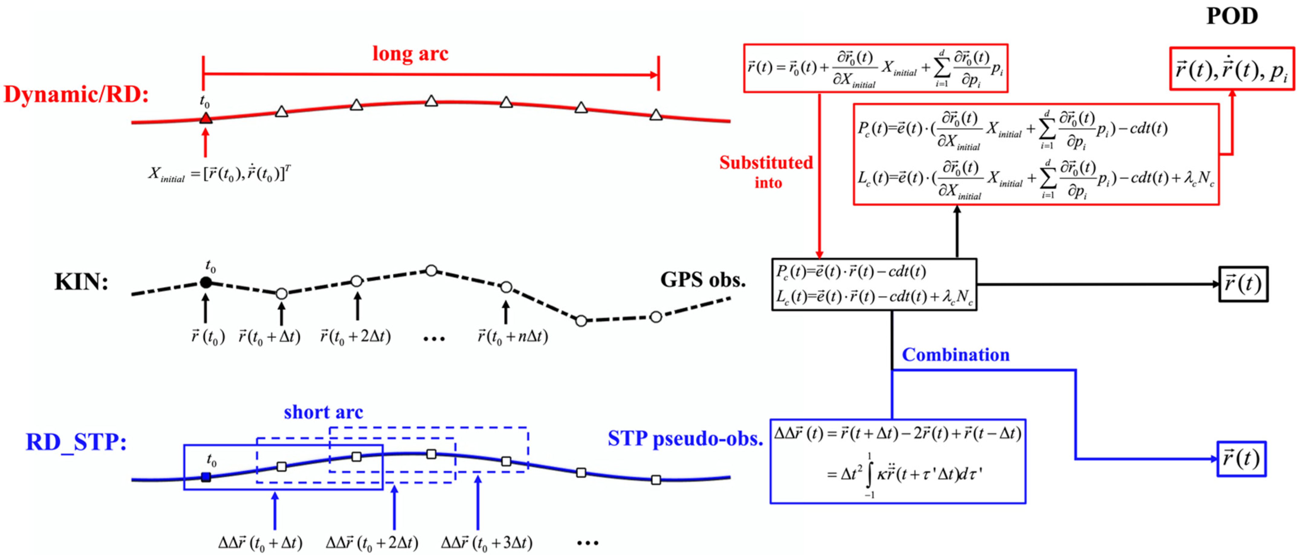
2.2. Kinematic Observation Equation

The dual-frequency code and carrier phase observations between the LEO satellite receiver (subscript L) and the GPS satellite PRN k (superscript Gk) at time epoch t can be described as follows [33]:
P i , L G k = ρ L , 0 G k + e L G k d r L + c ( d t G k d t L ) + α i I L G k + ε P i , L G k L i , L G k = ρ L , 0 G k + e L G k d r L + c ( d t G k d t L ) + λ i N i , L G k α i I L G k + ε i , L G k
where ρ L , 0 G k is the geometric distance between the GPS satellite’s true position r G k and the LEO satellite’s approximate position r L , 0 ; e L G k = r G k r L , 0 ρ L , 0 G k is the unit direction vector between the GPS and LEO satellites; d r L is the position correction vector d r L = r L r L , 0 , r L is the true position of the LEO satellite; c is the velocity of light in a vacuum; P i , L G k and L i , L G k are the dual-frequency code and carrier-phase observations, respectively; λ i and N i , L G k are the carrier-phase wavelength (in a vacuum) and ambiguity at frequency f i ( i = 1 , 2 ) , respectively; d t G k and d t L are the clock errors of the GPS and LEO satellite receivers, respectively; α 1 = 1 , α 2 = f 1 2 / f 2 2 , and I L G k is the ionospheric delay on L1; and ε P i , L G k and ε i , L G k are the code and carrier phase observation errors (e.g., multipath), respectively. Generally, r G k and d t G k can be obtained from the precise ephemeris and clock products released by CODE or the International GNSS Service (IGS) [34]. The relativistic effect and phase wind-up effect (due to the relative rotation between a transmitting and receiving antennas), which can be calculated using known correction models, are not shown in Equation (1). Moreover, for simplicity, subscript L, superscript Gk, ρ L , 0 G k , and d t G k are omitted in some of the following equations, without causing confusion.

2.3. New Dynamic Pseudo-Observation Equation

Newton’s equation of motion for LEOs in the inertial frame can be expressed as [6]
r ¨ = G M r r 3 + f ( t , r , r ˙ , p 1 , p d )
where G M is the gravitational constant times the Earth’s mass; r is the distance from the satellite to the Earth’s center; and r , r ˙ , and r ¨ are the position, velocity, and acceleration of the satellite, respectively. r ¨ includes Earth’s gravitation, Earth’s solid and ocean tidal forces, third body perturbations (e.g., luni-solar gravitation), perturbations due to the relativistic effect, atmospheric drag, solar radiation pressure, and Earth radiation pressure. p 1 , p d denote dynamical parameters considered as unknowns, e.g., scaling factors of analytically predicted accelerations.
In this paper, we propose to use the STP of LEOs as an additional dynamic “pseudo-observation”. Based on Equation (2), the STP equation for LEOs is derived (details shown in Appendix A) as follows [35]:
r ( t + Δ t ) 2 r ( t ) + r ( t Δ t ) = Δ t 2 1 1 κ r ¨ ( t + τ Δ t ) d τ
where
κ = { 1 τ 0 τ 1 1 + τ 1 τ < 0 , 0 κ 1   τ = τ t Δ t , t Δ t τ t + Δ t  
Δ Δ ( ) ( t ) = ( ) ( t + Δ t ) 2 ( ) ( t ) + ( ) ( t Δ t ) is the second-order time-difference operator, in which ( t + Δ t ) , ( t ) and ( t Δ t ) refer to three adjacent epochs. Δ Δ r ( t ) stands for r ( t + Δ t ) 2 r ( t ) + r ( t Δ t ) , which is the STP.
Equation (3) directly establishes the relationship between the positions at three adjacent epochs ( r ( t + Δ t ) , 2 r ( t ) , r ( t Δ t ) ) and accelerations r ¨ ( t ) . According to Equation (3), Δ Δ r ( t ) is only related to the in-arc acceleration r ¨ ( t ) and the square of the sampling interval Δ t 2 . The acceleration of LEOs r ¨ ( t ) in the inertial frame, which is the function of position, velocity, and time, can be computed precisely from the known dynamic models with the a priori orbit of LEOs [11,14,15,16]. Moreover, the errors caused by the unmodeled dynamic signals can be treated as the error sources of the STP “pseudo-observation”, and taken into account by the stochastic model of the STP “pseudo-observation”. The Δ Δ r ( t ) is computed by the numerical integration techniques used in the dynamic/RD method [36], and the practical procedure of the intergral STPs can refer to Section 3.1.2 in [35]. Therefore, combined with the kinematic observation equation, the intergrated STPs of LEOs can be used to estimate the precise positions of LEOs.

2.4. Function Model of the RD_STP Method

Combining Equations (1) and (3), the observation model of the RD_STP method for the POD of LEOs is expressed as follows:
P c , L G k ( t ) = e L G k ( t ) d r L ( t ) c d t L ( t ) + ε P c , L G k ( t ) L c , L G k ( t ) = e L G k ( t ) d r L ( t ) c d t L ( t ) + λ c N c , L G k + ε L c , L G k ( t ) Δ Δ d r L ( t ) = Δ Δ r L ( t ) Δ Δ r L , 0 ( t ) = Δ t 2 1 1 ( 1 | τ | ) r ¨ M ( t + τ Δ t ) d τ Δ Δ r L , 0 ( t ) + ε Δ Δ r L ( t )
where P c , L G k ( t ) and L c , L G k ( t ) are ionosphere-free linear combinations; Δ Δ r L is integrated via the right part of Equation (3); r ¨ M is the acceleration of the LEOs; and r L , 0 ( t ) is an a priori LEO orbit, e.g., from a code solution. Most of the force (e.g., Earth gravitation, luni-solar gravitation, tide forces) acting on LEOs is only function of time and position. Thus, the STPs Δ Δ r L can be computed precisely with the known dynamic models and an a priori LEO orbit r L , 0 ( t ) .
Linearizing Equation (4) yields the following:
y L G k = B L G k d X L G k + ε L G k
where
y L G k = [ P c , L G k ( t Δ t ) P c , L G k ( t ) P c , L G k ( t + Δ t ) L c , L G k ( t Δ t ) L c , L G k ( t ) L c , L G k ( t + Δ t ) Δ Δ d r L ] T
B L G k = [ e L G k ( t Δ t ) 0 0 1 0 0 0 0 e L G k ( t ) 0 0 1 0 0 0 0 e L G k ( t + Δ t ) 0 0 1 0 e L G k ( t Δ t ) 0 0 1 0 0 1 0 e L G k ( t ) 0 0 1 0 1 0 0 e L G k ( t + Δ t ) 0 0 1 1 2 1 0 0 0 0 0 1 2 1 0 0 0 0 0 1 2 0 0 0 0 ] } GPS   observations } STP   pseudo - observations
d X L G k = [ d r L ( t Δ t ) d r L ( t ) d r L ( t + Δ t ) c d t L ( t Δ t ) c d t L ( t ) c d t L ( t + Δ t ) λ c N c G k ] T
Here, Δ Δ d r L in Equation (5) are used as the additional “pseudo-observations” when estimating the satellites’ orbits, the receiver clock errors, and the carrier-phase ambiguities from the GPS observations ( P c , L G k ( t ) and L c , L G k ( t ) ). In the same way as in the kinematic method, the consecutive epochs are connected through the STP “pseudo-observations” and the phase observations. The carrier-phase ambiguities are estimated pass-dependently.
The stochastic model of the GPS observations uses the elevation-dependent weighting model, and sets σ L c G k = 0.01 ( m ) , σ P c G k = 1 ( m ) at the zenith direction. According to Equation (3), because 1 1 κ d τ = 1 , the stochastic model of the integrated STP pseudo-observation Δ Δ d r L is represented as follows:
σ Δ Δ d r L = σ r ¨ M Δ t 2 ( m )
where σ Δ Δ d r L is the RMS of the errors of Δ Δ d r L , and the unit is meters; and σ r ¨ M is the RMS of the errors of the dynamic models including the noise in the used dynamic models and the unmodeled dynamic signals (e.g., luni-solar gravitation) in the RD_STP method.
Here, we assume that the STP pseudo-observations and the GPS observations are independent of each other. Then, based on Equations (3)–(6), the three-dimensional coordinate corrections, receiver clock bias, and ambiguity can be estimated via the least-squares method from the code, carrier-phase observations, and STP pseudo-observations.

2.5. Characteristics of the RD_STP Method

Based on Equation (2), the actual orbit of LEOs r L ( t ) in the traditional dynamic/RD method is expressed as follows [6]:
r L ( t ) = r L , 0 ( t ) + r L , 0 ( t ) X i n i t i a l X i n i t i a l + i = 1 d r L , 0 ( t ) p i p i
where X i n i t i a l = [ r L ( t 0 ) , r ˙ L ( t 0 ) ] T stands for the LEO satellite’s initial conditions at epoch t 0 ; p i , i = 1 , 2 , , d denote the unknown dynamical parameters; and r L , 0 ( t ) X i n i t i a l and r L , 0 ( t ) p i are the partial derivatives of the a priori orbit r L , 0 ( t ) to the satellite’s initial conditions and the dynamical parameters, respectively. The errors caused by the unmodeled dynamic signals are absorbed by the unknown dynamical parameters or pseudo-stochastic orbit parameters.
It is obvious that both the STP equation Equation (3) in the RD_STP method and Equation (7) in the traditional dynamic/RD method are based on Newton’s equation of motion. However, compared with the dynamic/RD method, the essence of the RD_STP method is that the STPs are taken as an additional dynamic “pseudo-observation” with errors to constrain the GPS observations. Moreover, all the unmodeled dynamic signals are treated as the error sources of the STP pseudo-observation, rather than absorbed by the unknown dynamical parameters or pseudo-stochastic orbit parameters.
The main characteristics of the RD_STP method for the POD of LEOs are summarized in Table 1. For comparison, the characteristics of the kinematic, dynamic, and RD POD methods are also given in Table 1 and shown in Figure 1. As shown, the RD_STP method has four main differences compared with the dynamic and RD methods. First, the RD_STP method integrates the acceleration over a very short arc (e.g., 2 Δ t = 60   s ) to compute the STPs, while the dynamic and RD methods usually use the long-arc integration (e.g., 24 h or 30 h) [11], Thus, the short-arc integration reduces the accuracy requirements for the dynamic models. Second, the known minor perturbation forces (e.g., Earth’s solid and ocean tidal forces, third body perturbation, and the non-conservative forces) can be ignored if the sampling interval is less than 30 s. Third, an Earth’s gravity field model with low degree and order (e.g., up to degree and order 90) is sufficient, even for LEOs. Certainly, similar to the dynamic/reduced-dynamic method, the perturbation forces (<10−5 ms−2) can be taken into account for integrating the STPs into the proposed RD_STP method as well, if a stronger dynamic constraint on the POD solutions is desired. Finally, there are no dynamic parameters or pseudo-stochastic parameters to be estimated in the proposed method.
Moreover, the RD_STP method can easily adjust the strength of the dynamic constraints on the GPS observations by modifying the stochastic model of the STP pseudo-observations in Equation (6). When σ r ¨ M = in Equation (6), which means that the weight of the constraint in Equation (5) is infinitesimally small, the RD_STP method will degenerate into the kinematic method.

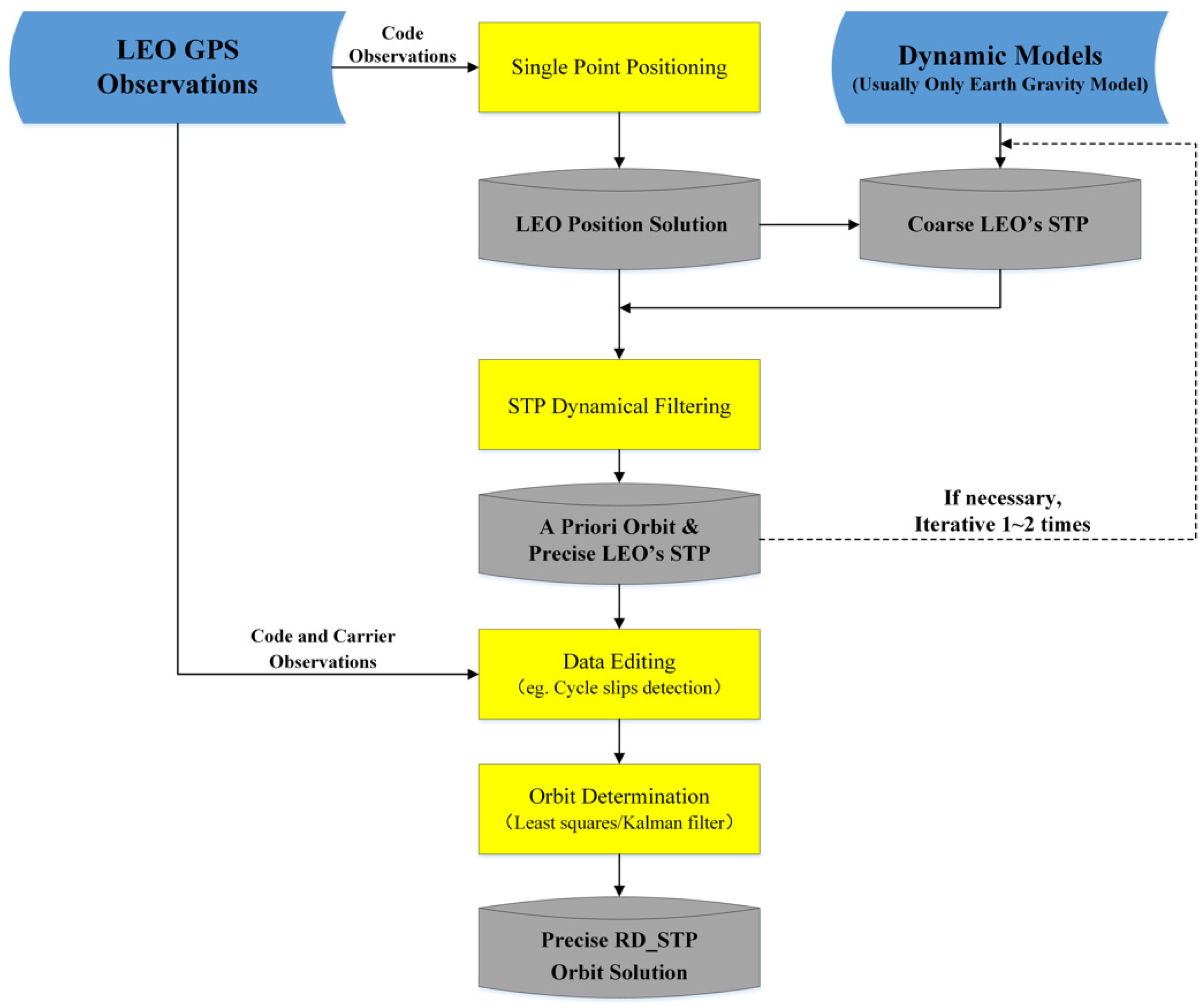
2.6. Steps of the RD_STP Method for POD

Figure 2 shows the simplified processing scheme of the RD_STP method for the POD of LEOs from GPS observations, which is described as follows.
Step 1, The GPS code observations of LEOs are used to estimate the positions of the LEO via the single-point positioning approach.
Step 2, The coarse STPs of LEOs are computed from the estimated positions in Step 1 and an a priori dynamic model (usually only Earth’s gravity field, e.g., EGM2008 up to degree and order 90) based on Equation (3). Moreover, when there is a data gap Δ t g a p , the corresponding STP will be set as r ( t + Δ t g a p ) 2 r ( t ) + r ( t Δ t g a p ) with an STP error according to Equation (6).
Step 3, An a priori orbit is estimated from the code and the coarse STP pseudo-observations generated in Steps 1 and 2 based on Equations (4)–(6), which is called the STP dynamical filtering in Figure 2.
Note that, sometimes, there are gross errors in the code observations, and the error of the estimated LEO’s positions in Step 1 has an influence on computing the accelerations. Thus, the iterative processing procedure may be necessary in Step 3. In general, 1–2 iterations are enough. The accuracy of the generated a priori orbit is usually better than 1 m, which can meet the requirements for STP “pseudo-observations”. Then, the precise LEO’s STP pseudo-observations are integrated based on the a priori dynamic model and the a priori orbit after several iterations.
Step 4, The GPS code and carrier observations are screened and edited (e.g., detecting cycle slips) based on the method used by [23], according to the a priori orbit and precise STPs generated in Step 3.
Step 5, The RD_STP POD of LEOs is estimated via the least squares adjustment/Kalman filter method based on Equations (4)–(6).
The POD solution does not need any external reference orbit for initialization, and is fully self-contained. The performance of the proposed RD_STP method will be assessed in the following section.

3. Results

In this section, the influences of the sampling interval and the a priori dynamic models on the accuracies of integrating the STPs of satellite will be analyzed according to the accuracy requirement of 0.01 m for the STPs, which is sufficient for the POD of LEOs, such as GOCE [37]. Moreover, the RD_STP method will be applied to process the real GPS observations of GOCE, and the POD results will be discussed in detail.

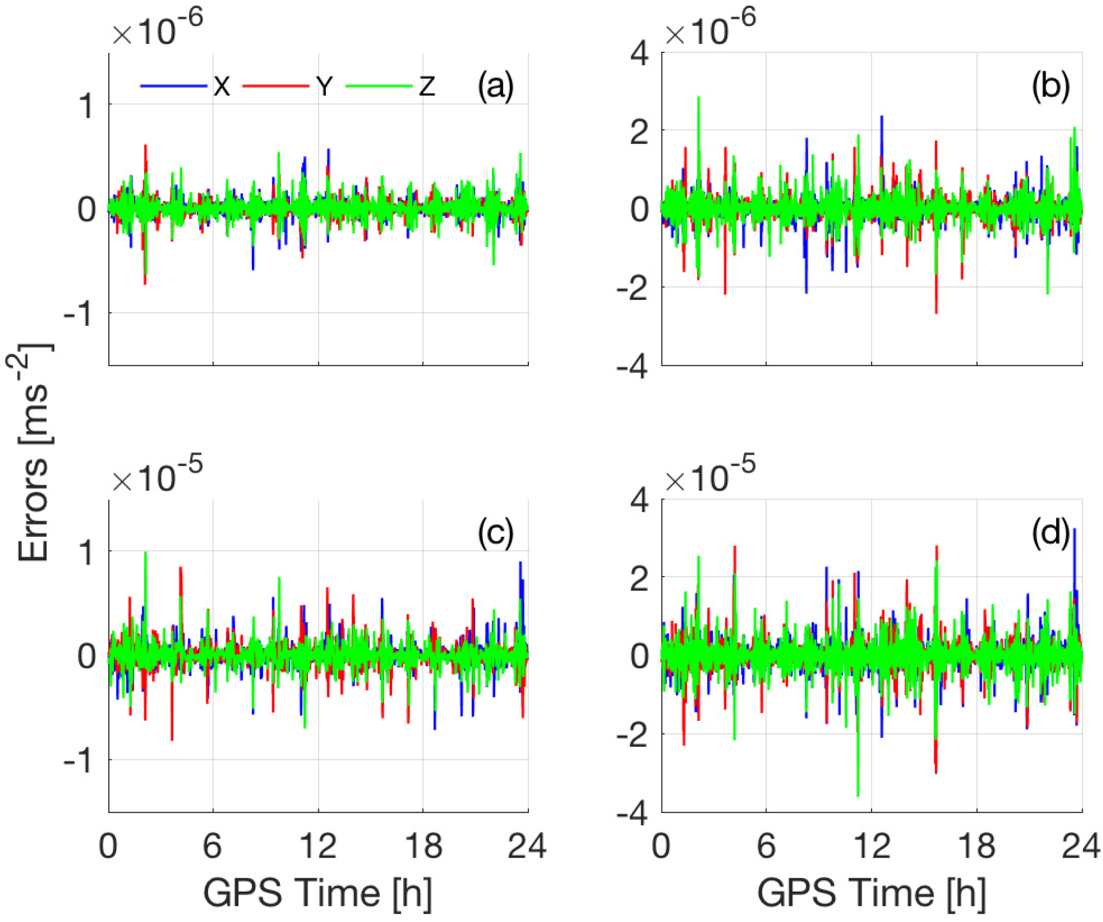
3.1. Accuracy Analysis of the Integrated STP Pseudo-Observations

To analyze the influences of the dynamic models and the sampling interval on the accuracy of integrating STPs, we choose the one-day reduced-dynamic POD solution of the GOCE satellite (orbital altitude of approximately 260 km) [31,32], and the GRACE A/B satellites (orbital altitude of approximately 500 km) provided by the Jet Propulsion Laboratory [38]. The RD POD solutions are used as the true orbit.

3.1.1. Influence of the Sampling Interval

To analyze the influence of the sampling interval on the accuracy of the STP, we first set up the relationship σ r ¨ = 0.01 Δ t 2 based on Equation (3), corresponding to an accuracy requirement of 0.01 m on the STP. According to σ r ¨ = 0.01 Δ t 2 , the accuracy requirement for a priori accelerations increases as the sampling interval increases. If the a priori acceleration errors are less than 10−5 ms−2, the error of the computed STP is less than 0.01 m, even for a sampling interval of 30 s. For a sampling interval of 10 s, the accuracy of the a priori accelerations should be better than 10−4 ms−2. Fortunately, the errors or magnitudes of the accelerations of many dynamic models of LEOs are below 10−4 ms−2, which will be discussed in the following section.

3.1.2. Magnitude and Error of the a Priori Dynamic Models

Because the a priori orbit error has an influence on computing the accelerations, its influence should be analyzed first. Here, we suppose the a priori orbit error δ r is 3   m , which is worse than the accuracy of a GPS code orbit solution [39]. We only analyze the error ( δ a ) in the computation of the Earth’s center gravitation accelerations owing to the a priori orbit error, because its magnitude is far larger than the other forces. The error δ a is δ a g r δ r 5 × 10 6   ms 2 < 10 5   ms 2 , where g 9.8   ms 2 . Therefore, δ a can be ignored, even for a sampling interval of 30 s. In addition, when a more precise a priori orbit is necessary, the iterative processing procedure can be applied (see Figure 2).
Figure 3 shows the GOCE’s accelerations from the known conservative force models except for the EGM, including luni-solar gravitation (DE405), ocean tide, solid Earth tide, ocean pole tide, and solid pole tide (IERS2010) [40]. According to Figure 3, the accelerations of all conservative force models except for the EGM are less than 10−6 ms−2. Therefore, even if we ignore these known conservative force models, the influence on the computed STP is less than 1 mm for a sampling interval of less than 30 s.
Because the Earth’s gravitation acting on the LEOs is far larger than 10−5 ms−2, it cannot be ignored in computing the STP for an accuracy requirement of 0.01 m. However, the maximum degree of the EGM, which could satisfy the accuracy requirement of computing the STP, should be analyzed. We use the EGM2008 (up to degree and order 180) [41] as the reference model to analyze the omission errors of the accelerations for different maximum degrees (60, 90, 120, and 150), which are shown in Figure 4. According to Figure 4, the omission errors of the EGM2008 model up to degree and order 90 are less than 10−5 ms−2 for GOCE, which indicates that the EGM up to degree and order 90 is sufficient for computing the STPs with an accuracy of 0.01 m when Δt = 30 s.
Moreover, according to previous studies [11,42,43], the non-conservative forces acting on the satellites with very low orbits (e.g., CHAMP, GRACE, and GOCE) are usually less than 10−5 ms−2. Therefore, for integrating the STPs with an accuracy of 0.01 m, the non-conservative forces acting on the LEOs can be ignored as well, which usually cannot be neglected in dynamic or RD orbit determinations [42,43].
From the above analysis, for an accuracy requirement of 0.01 m for the integrated STP, all perturbation forces except Earth’s gravitation acting on the GOCE satellite could be ignored for a sampling interval less than or equal to 30 s. It should be noted that all the unmodeled dynamic signals here will be taken into account by the stochastic model of the STP “pseudo-observations”. Moreover, the EGM2008 model up to degree and order 90 is sufficient for integrating the STPs of the GOCE satellite with an accuracy of better than 0.01 m.

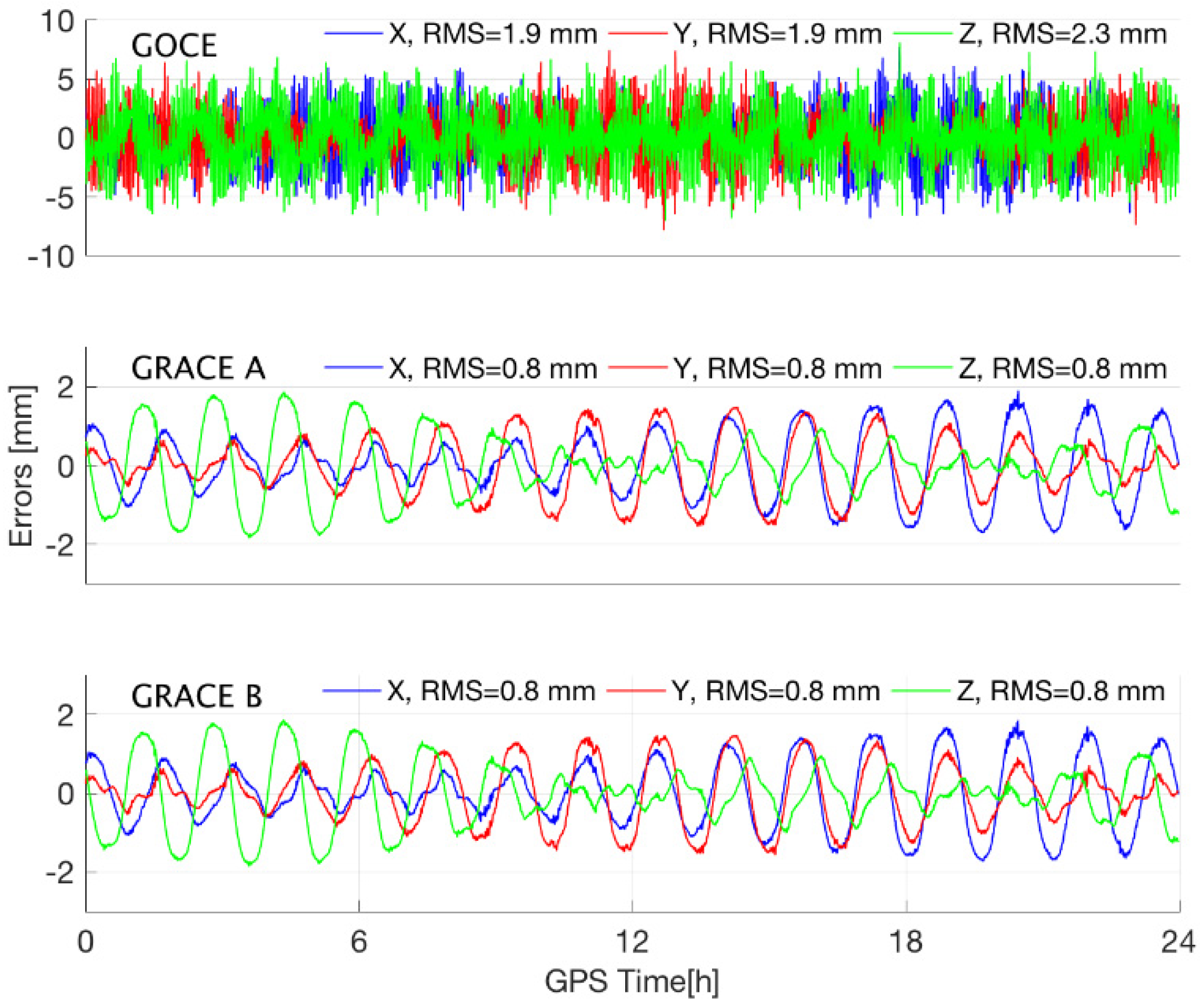
3.1.3. Accuracy Analysis of Integrating the STPs of GOCE and GRACE

We only use the EGM2008 model up to degree and order 90 to establish the STPs of GOCE and GRACE A/B satellites with a sampling interval of 30 s. The STPs computed from the RD POD solutions (left part of Equation (3)) are used as the “true values” to validate the integrated STPs (right part of Equation (3)) from the EGM2008 model and the RD POD solutions. The errors of the integrated STPs with a sampling interval of 30 s are shown in Figure 5. According to the figure, the errors of the three coordinate components (x, y, z) are far less than 0.01 m, and the corresponding RMS are 1.9 mm, 1.9 mm, and 2.3 mm for GOCE, respectively, and 0.8 mm, 0.8 mm, and 0.8 mm for GRACE A/B, respectively. The errors of the computed STPs of GOCE are larger than those of GRACE because the ignored gravitational accelerations (e.g., ocean tide, solid tide) of GOCE are larger than those of GRACE owing to the lower orbital altitude of GOCE. However, the STP accuracies of GRACE and GOCE are much better than 0.01 m, consistent with the previous conclusions in Section 3.1.2.
Figure 6 shows the three-dimensional root mean square (3D RMS) of the GOCE’s STP errors corresponding to EIGEN5S [44] and EGM2008 with different maximum degrees and orders, and different sampling intervals. According to Figure 6, the differences between the results that correspond to EIGEN5S and EGM2008 are negligible, even with a sampling interval of 300 s and a maximum degree and order up to 150. The RMS of the STP errors increases as the sampling interval increases. Further, although the RMS of the STP errors decreases as the degree increases, the reduction after 90 degrees is very limited, consistent with the results shown in Figure 4. Therefore, only EGM2008 up to degree and order 90 is set as the only a priori dynamic model in the real data processing.
As stated above, the acceleration errors caused by only using the EGM2008 up to degree and order 90 are less than 10−5 ms−2. Therefore, we set σ r ¨ M = 10 5   ms 2 . Based on Equation (3), the corresponding error of Δ Δ d r L with a sampling interval of 30 s is 9 mm, which is much larger than the “true” errors shown in Figure 5. Thus, the assumption of a stochastic model for Δ Δ d r L is moderate, which will reduce the influence of the a priori dynamic model on the RD_STP solution.

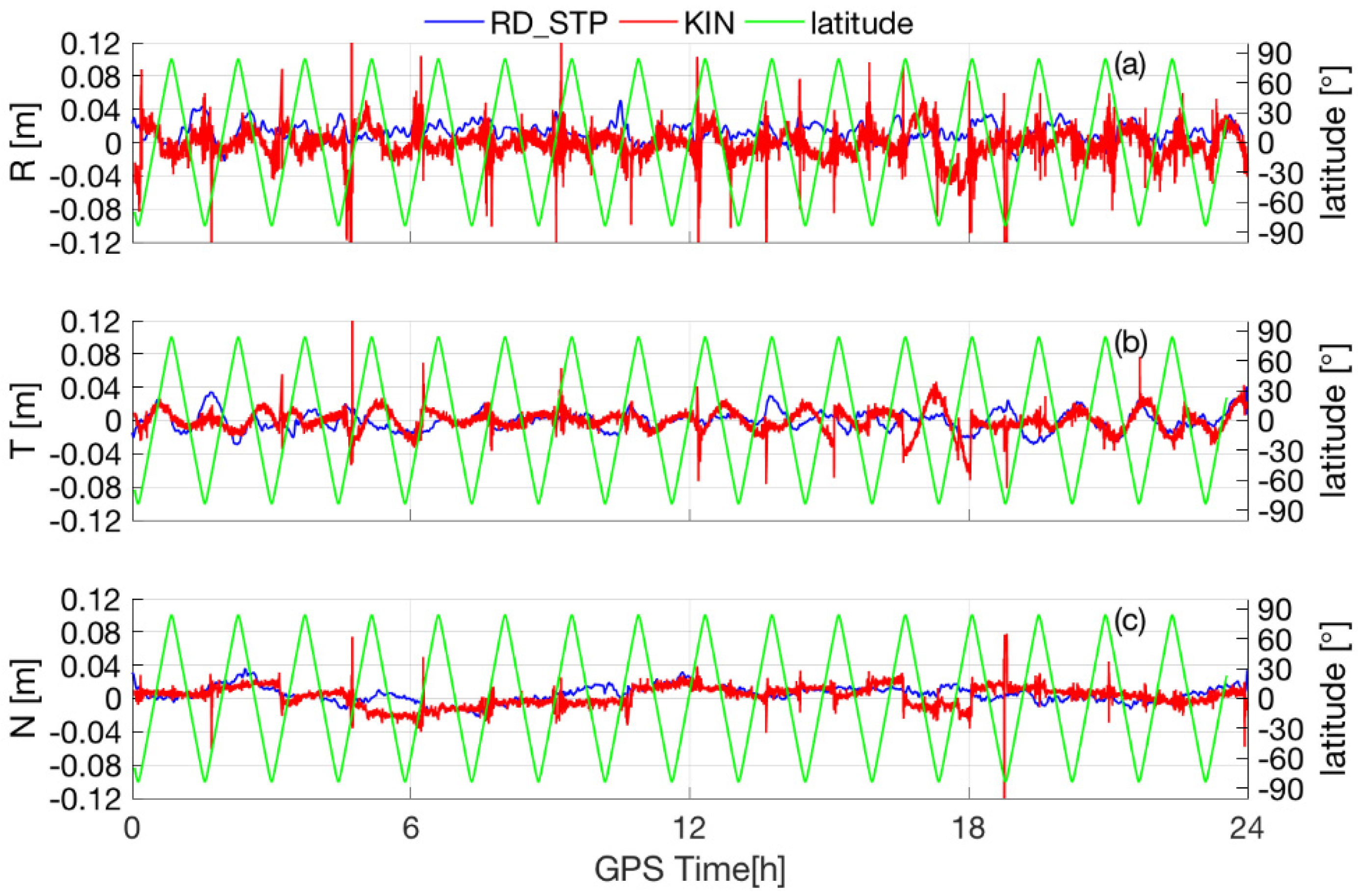
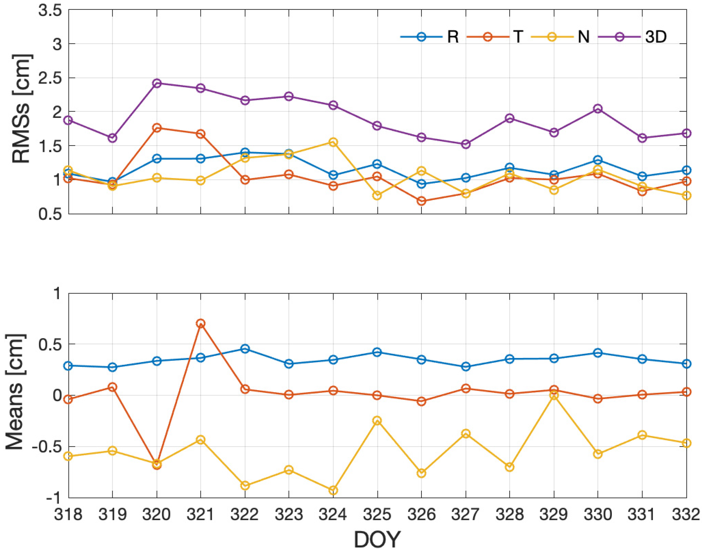
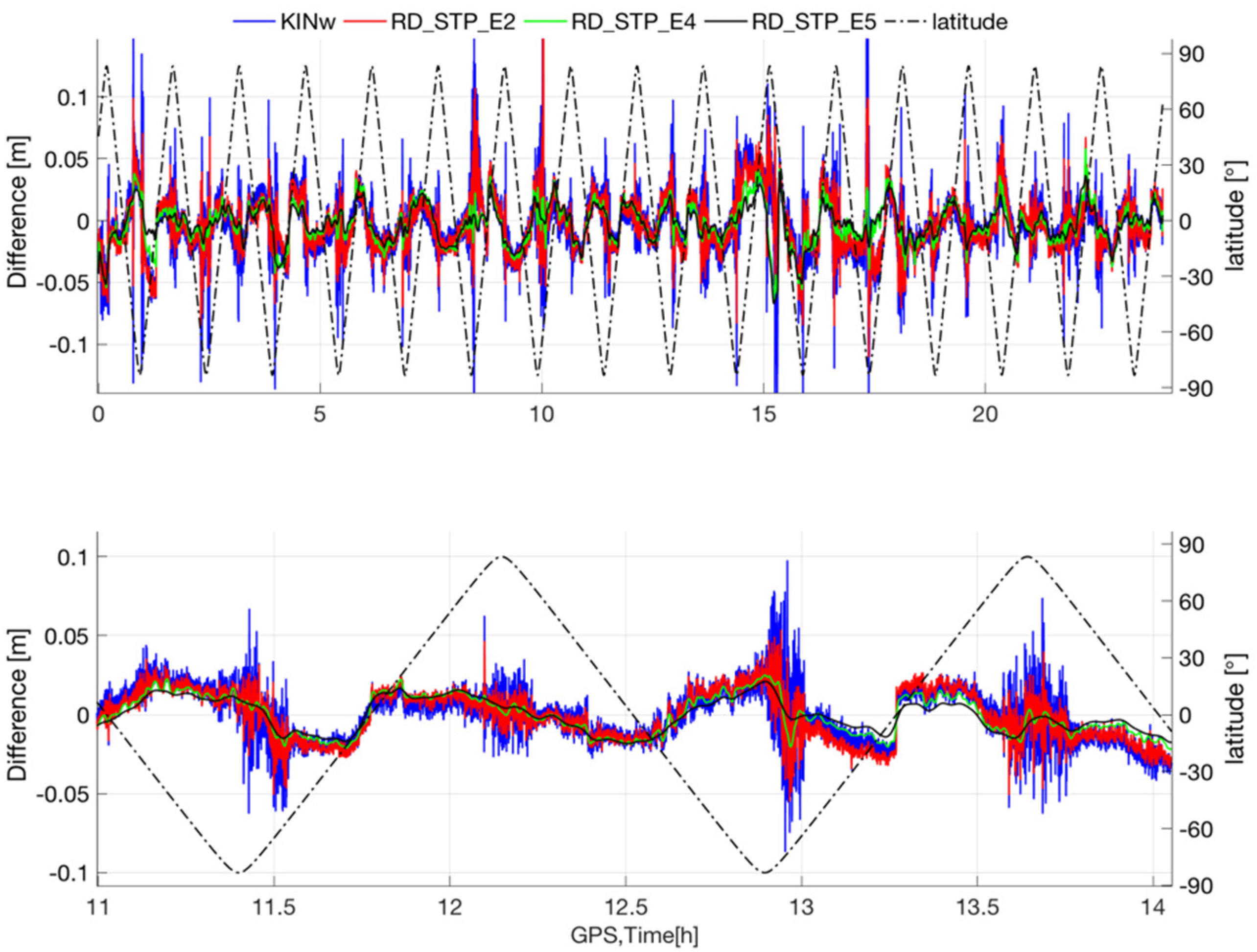
3.2. POD of GOCE Satellite Based on the RD_STP Method

The parameter settings for the RD_STP POD of GOCE are listed in Table 2. For comparison, the parameters used by Bock et al. [11] are also listed in the table. Moreover, because the released kinematic solutions of GOCE are provided at a sampling rate of 1 Hz, it is reasonable to choose Δ t = 1 s in the RD_STP POD. Thus, the RMS error of the GOCE’s 1 s STP pseudo-observation is set as σ Δ Δ d r L = 10 5   m according to Equation (3), when σ r ¨ M = 10 5   ms 2 .

POD Results and Analysis

Using the preprocessed data, the precise orbits are determined via the RD_STP method based on the self-developed low-orbit satellite orbit determination software. For the evaluation of the 1s RD_STP solutions, here, we use the RD solutions as the “true” values of the satellite orbit.
The errors of the 1s RD_STP solutions in the radial (R), along-track (T), and normal component (N) directions are shown in Figure 7. The errors of the KIN solutions and the latitudes of the satellite are also shown in Figure 7. According to the figure, the 1s RD_STP solutions are smoother than the KIN solutions because the dynamic contraint is applied and the solutions are closer to the RD solutions. Because the assumption of σ r ¨ M = 10 5   ms 2 is much larger than the true errors (shown in Section 3.1.3), the dynamic constraints from the STPs are not as strong as those in the traditional RD method. This outcome means that the RD_STP solutions are not intended to approach the RD solutions. In addition, the systematic differences between the RD_STP and RD solutions are possibly caused by the differences of the a priori dynamic models used here, and the orbit determination software platforms (e.g., the cycle slip detection method).
The daily means and RMSs of the differences between the 1s RD_STP solutions and the RD solutions for the selected 15 days are shown in Figure 8. According to Figure 8, all 15 24–h RMSs are less than 2 cm with nearly zero means in the three directions (R, T, N), and their mean 3D RMS is 1.93 cm. This outcome indicates that the RD_STP method performs very well, and the accuracy of its solutions is consistent with that of the RD solutions.
To further analyze the influences of the a priori gravity field model and the statistical model on the RD_STP solutions, Figure 9 shows the differences of the RD_STP solutions with the different dynamic constraints corresponding to the EGM2008 and EIGEN5S models at a specific time interval of 3 h at DOY 330, 2009. The maximum degree and order of EGM2008 and EIGEN5S is set to 90, and the root of the noise variance of the accelerations computed from these two models is set to 10−5 ms−2. According to Figure 9, the differences are less than 0.5 mm for the R, T, and N directions, illustrating that the RD_STP POD solutions are not so sensitive to the a priori gravity field model, and the assumption of the stochastic model for the STP pseudo-observation is reasonable. This outcome is consistent with the conclusion given in Section 3.1.3. Moreover, the differences in the radial direction are larger than the ones in the other directions, which is reasonable because the acceleration differences between EGM2008 and EIGEN5S in the radial direction are biggest.
To analyze the influences of the relative weights of the STPs, we estimated several RD_STP solutions corresponding to the different stochastic models at DOY 319 of 2009, the radial differences (compared with the RD solutions) of the KIN solutions, and the RD_STP solutions are shown in Figure 10. As with the previous experiment, the EGM2008 model up to degree and order 90 is also used as the a priori dynamic model. The blue solid line in Figure 10 represents the differences of the kinematic solutions (named KINw) estimated by our own software. Further, the red solid line, green solid line, and black solid line represent the differences of the RD_STP solutions with the stochastic models σ Δ Δ d r L = 10 2 Δ t 2 ( m ) (named RD_STP_E2), σ Δ Δ d r L = 10 4 Δ t 2 ( m ) (RD_STP_E4), and σ Δ Δ d r L = 10 5 Δ t 2 ( m ) (RD_STP_E5), respectively. According to Figure 10, when the noise of the accelerations computed from EGM 2008 is set to be larger, which means a smaller weight for the STP pseudo-observations, the KINw and the RD_STP solutions are very close to each other (see the blue solid line and red solid line in Figure 10). Therefore, the RD_STP solutions will be exactly the same as the kinematic solutions when the weight of the STP pseudo-observations is small enough. Moreover, the larger weight (smaller σ Δ Δ d r L ) of the statistical model produces a smoother solution, especially in nearly polar and equatorial regions (see the green and black solid line in Figure 10). This is consistent with the findings of Bock et al. [12], who showed that there are systematic errors in GOCE orbits in those regions. This outcome indicates that the STP pseudo-observations have a stronger dynamic constraint when the quality of on-board GPS data is poor.
In addition, GOCE POD solutions for DOY 318~332 of 2009 with 10 s and 30 s sampling are generated as well. The mean RMSs of the differences between the solutions (KIN-10 s, KIN-30 s, RD_STP-10 s, and RD_STP-30 s) and the RD solutions are shown Table 3. According to Table 3, for the same sampling intervals, the RD_STP solutions are smoother than the KIN solutions, and closer to the RD solutions. Moreover, when the sampling interval is smaller, the RD_STP solutions are closer to the RD solutions. This is similar to the POD results of 1 s sampling. The 15-day mean 3D RMS of the differences between the RD_STP and RD solutions is 2.77 cm for 30 s sampling and 2.53 cm for 10 s sampling.

4. Conclusions

Differing from the traditional dynamic/RD method and the kinematic method, we propose a new reduced-dynamic method for the POD of LEOs using GPS code and carrier phase observations. Given that the STP directly establishes the relationship between the position and acceleration of the LEOs, and can be easily and precisely computed from known dynamic models, we used it as an additional “pseudo-observation” equation for the dynamic constraint on the kinematic POD observation equation. Moreover, all the unmodeled dynamic signals are taken into account by the stochastic model of the STP “pseudo-observations” in the RD_STP method, rather than being absorbed by the unknown dynamical parameters or pseudo-stochastic orbit parameter.
The theoretical and numerical analyses show that, when the accuracy of the a priori force models is 10−5 ms−2 over a short time span (e.g., 2 Δ t = 60 s ), the accuracy of the integrated STPs is better than 0.01 m, which is good enough for the POD of LEOs. Therefore, compared with the traditional dynamic/RD method, the minor perturbation forces with a magnitude less than 10−5 ms−2 (such as luni-solar gravitation, tidal forces, and atmospheric drag) acting on the satellite can be ignored and treated as the error sources of the STP pseudo-observation. Further, only the Earth’s gravity field model (such as EGM2008, EIGEN5S) up to degree and order 90 is sufficient for the POD because its omission errors are less than 10−5 ms−2. This outcome means that the dependence of the RD_STP method on Earth’s gravity field model is reduced compared with the traditional dynamic/RD method.
The POD experiment of GOCE based on the RD_STP method shows that the RD_STP solution is consistent with the RD solution in terms of accuracy and is more accurate and smoother than the KIN solution in the regions near the equator and poles. The 3D RMS of the differences between the RD_STP and RD solutions is 1.93 cm, 2.53 cm, and 2.77 cm for 1 s, 10 s, and 30 s sampling, respectively.
These experimental results indicate that the RD_STP method is effective and can be an alternative for the POD of LEOs. In addition, if σ Δ Δ d r L = , the RD_STP method would be exactly equivalent to the kinematic method, which means that the RD_STP solutions have nothing to do with the a priori dynamic model. Thus, the RD_STP method can adjust the influence of the dynamic information on the POD solutions by modifying the stochastic model of the STP pseudo-observations, and might also be an alternative to estimating the orbits in the context of gravity field determination such as the highly-reduced-dynamic orbits [7].

Author Contributions

Conceptualization, H.W. and X.X.; Data curation, H.W. and K.K.; Formal analysis, H.W.; Funding acquisition, H.W., J.L. and X.X.; Investigation, H.W.; Methodology, H.W. and J.L.; Resources, H.W. and J.L.; Software, H.W., S.Z. and K.K.; Validation, X.X.; Writing—original draft, H.W. and X.X.; Writing—review & editing, H.W. and X.X. All authors have read and agreed to the published version of the manuscript.

Funding

This research was funded by the Foundation for Innovative Research Groups at the National Natural Science Foundation of China (grant no. 41721003), the National Natural Science Foundation of China (grant no. 41774020,42074019), the German Academic Exchange Service (DAAD) Thematic Network Project (grant no. 57421148), and the fellowship of China National Postdoctoral Program for Innovative Talents (grant no. BX20200251).

Data Availability Statement

The GOCE data in this study are available in “http://earth.esa.int/GOCE/ (accessed on 16 May 2018)” and the GPS data are obtained in “http://ftp.aiub.unibe.ch/CODE/ (accessed on 25 March 2018)”.

Acknowledgments

The authors acknowledge the European Space Agency for providing the GOCE data and the Center for Orbit Determination in Europe for providing the GPS data. We are also grateful to the anonymous reviewers and the associate editor for their comments and suggestions.

Conflicts of Interest

The authors declare no conflict of interest.

Appendix A

The following content in Appendix A includes the detailed descriptions of the derivation of the LEO’s STP equation.
First, based on the Newton’s equation of motion, the actual position of the LEOs at epoch t + Δ t can be expressed as follows:
r ( t + Δ t ) = r ( t ) + r ˙ ( t ) Δ t + t t + Δ t t t r ¨ ( τ ) d τ d t
where r ( t ) , r ˙ ( t ) , and r ¨ ( t ) are the LEO’s position, velocity, and acceleration at epoch t and Δ t is the time interval.
By changing the integration order in Equation (A1), we find the following:
r ( t + Δ t ) = r ( t ) + r ˙ ( t ) Δ t + t t + Δ t ( t + Δ t τ ) r ¨ ( τ ) d τ
Similarly, we can formulate the equation for the negative:
r ( t Δ t ) = r ( t ) r ˙ ( t ) Δ t + t t Δ t ( t Δ t τ ) r ¨ ( τ ) d τ
Thus, based on Equations (A2) and (A3), the STP equation for LEOs is derived as follows [35]:
r ( t + Δ t ) 2 r ( t ) + r ( t Δ t ) = t Δ t t + Δ t ( Δ t | τ t | ) r ¨ ( τ ) d τ = Δ t 2 1 1 ( 1 | τ | ) r ¨ ( t + τ Δ t ) d τ = Δ t 2 1 1 κ r ¨ ( t + τ Δ t ) d τ
where
κ = { 1 τ 0 τ 1 1 + τ   1 τ < 0 , 0 κ 1   τ = τ t Δ t , t Δ t τ t + Δ t  
Δ Δ ( ) ( t ) = ( ) ( t + Δ t ) 2 ( ) ( t ) + ( ) ( t Δ t ) is the second-order time-difference operator, in which ( t + Δ t ) , ( t ) , and ( t Δ t ) refer to three adjacent epochs. Δ Δ r ( t ) ; is the STP.
According to Equation (A4), Δ Δ r ( t ) is only related to the in-arc acceleration r ¨ ( t ) and the square of the sampling interval Δ t 2 . The STP equation Equation (A4) directly establishes the relationship between the positions at three adjacent epochs ( r ( t + Δ t ) , 2 r ( t ) , r ( t Δ t ) ) and accelerations r ¨ ( t ) .

References

  1. Bertiger, W.I.; Bar-Sever, Y.E.; Christensen, E.J.; Davis, E.S.; Guinn, J.R.; Haines, B.J.; Ibanez-Meier, R.W.; Jee, J.R.; Lichten, S.M.; Melbourne, W.G.; et al. GPS precise tracking of TOPEX/POSEIDON: Results and implications. J. Geophys. Res. Space Phys. 1994, 99, 24449–24464. [Google Scholar] [CrossRef]
  2. Luthcke, S.B.; Zelensky, N.P.; Rowlands, D.D.; Lemoine, F.G.; Williams, T.A. The 1-Centimeter Orbit: Jason-1 Precision Orbit Determination Using GPS, SLR, DORIS, and Altimeter Data Special Issue: Jason-1 Calibration/Validation. Mar. Geod. 2003, 26, 399–421. [Google Scholar] [CrossRef]
  3. Cerri, L.; Berthias, J.P.; Bertiger, W.I.; Haines, B.J.; Lemoine, F.G.; Mercier, F.; Ries, J.C.; Willis, P.; Zelensky, N.P.; Ziebart, M. Precision Orbit Determination Standards for the Jason Series of Altimeter Missions. Mar. Geod. 2010, 33, 379–418. [Google Scholar] [CrossRef]
  4. Flohrer, C.; Otten, M.; Springer, T.; Dow, J. Generating precise and homogeneous orbits for Jason-1 and Jason-2. Adv. Space Res. 2011, 48, 152–172. [Google Scholar] [CrossRef]
  5. Bisnath, S. Precise Orbit Determination of Low Earth Orbiters with a Single GPS Receiver-Based. Geometric Strategy. Ph.D. Dissertation, Department of Geodesy and Geomatics Engineering, University of New Brunswick, Fredericton, NB, Canada, 2004; 143p. [Google Scholar]
  6. Jäggi, A.; Hugentobler, U.; Beutler, G. Pseudo-Stochastic Orbit Modeling Techniques for Low-Earth Orbiters. J. Geod. 2006, 80, 47–60. [Google Scholar] [CrossRef] [Green Version]
  7. Jäggi, A.; Beutler, G.; Bock, H.; Hugentobler, U. Kinematic and highly reduced-dynamic LEO orbit determination for gravity field estimation. In International Symposium on Earth and Environmental Sciences for Future Generations; Springer Science and Business Media LLC: Berlin/Heidelberg, Germany, 2008; pp. 354–361. [Google Scholar]
  8. Jäggi, A.; Hugentobler, U.; Bock, H.; Beutler, G. Precise orbit determination for GRACE using undifferenced or doubly differenced GPS data. Adv. Space Res. 2007, 39, 1612–1619. [Google Scholar] [CrossRef]
  9. Jäggi, A.; Dach, R.; Montenbruck, O.; Hugentobler, U.; Bock, H.; Beutler, G. Phase center modeling for LEO GPS receiver antennas and its impact on precise orbit determination. J. Geod. 2009, 83, 1145–1162. [Google Scholar] [CrossRef] [Green Version]
  10. Montenbruck, O.; Andres, Y.; Bock, H.; Van Helleputte, T.; Ijssel, J.V.D.; Loiselet, M.; Marquardt, C.; Silvestrin, P.; Visser, P.; Yoon, Y. Tracking and orbit determination performance of the GRAS instrument on MetOp-A. GPS Solut. 2008, 12, 289–299. [Google Scholar] [CrossRef] [Green Version]
  11. Bock, H.; Jäggi, A.; Meyer, U.; Visser, P.; Ijssel, J.V.D.; Van Helleputte, T.; Heinze, M.; Hugentobler, U. GPS-derived orbits for the GOCE satellite. J. Geod. 2011, 85, 807–818. [Google Scholar] [CrossRef] [Green Version]
  12. Bock, H.; Jaggi, A.; Beutler, G.; Meyer, U. GOCE: Precise orbit determination for the entire mission. J. Geod. 2014, 88, 1047–1060. [Google Scholar] [CrossRef]
  13. Ijssel, J.V.D.; da Encarnacao, J.T.; Doornbos, E.; Visser, P. Precise science orbits for the Swarm satellite constellation. Adv. Space Res. 2015, 56, 1042–1055. [Google Scholar] [CrossRef]
  14. Jäggi, A.; Dahle, C.; Arnold, D.; Bock, H.; Meyer, U.; Beutler, G.; Ijssel, J.V.D. Swarm kinematic orbits and gravity fields from 18 months of GPS data. Adv. Space Res. 2016, 57, 218–233. [Google Scholar] [CrossRef]
  15. Montenbruck, O.; Hackel, S.; Ijssel, J.V.D.; Arnold, D. Reduced dynamic and kinematic precise orbit determination for the Swarm mission from 4 years of GPS tracking. GPS Solut. 2018, 22, 79. [Google Scholar] [CrossRef]
  16. Montenbruck, O.; Hackel, S.; Jäggi, A. Precise orbit determination of the Sentinel-3A altimetry satellite using ambiguity-fixed GPS carrier phase observations. J. Geod. 2018, 92, 711–726. [Google Scholar] [CrossRef] [Green Version]
  17. Švehla, D.; Rothacher, M. Kinematic positioning of LEO and GPS satellites and IGS stations on the ground. Adv. Space Res. 2005, 36, 376–381. [Google Scholar] [CrossRef]
  18. Geng, J.; Teferle, F.N.; Meng, X.; Dodson, A.H. Kinematic precise point positioning at remote marine platforms. GPS Solut. 2010, 14, 343–350. [Google Scholar] [CrossRef]
  19. Li, J.; Zhang, S.; Zou, X.; Jiang, W. Precise orbit determination for GRACE with zero-difference kinematic method. Chin. Sci. Bull. 2010, 55, 600–606. [Google Scholar] [CrossRef]
  20. Weinbach, U.; Schön, S. Improved GRACE kinematic orbit determination using GPS receiver clock modeling. GPS Solut. 2013, 17, 511–520. [Google Scholar] [CrossRef]
  21. Baur, O.; Bock, H.; Höck, E.; Jäggi, A.; Krauss, S.; Mayer-Gürr, T.; Reubelt, T.; Siemes, C.; Zehentner, N. Comparison of GOCE-GPS gravity fields derived by different approaches. J. Geod. 2014, 88, 959–973. [Google Scholar] [CrossRef]
  22. Zehentner, N.; Mayer-Gürr, T. Precise orbit determination based on raw GPS measurements. J. Geod. 2016, 90, 275–286. [Google Scholar] [CrossRef] [Green Version]
  23. Montenbruck, O.; van Helleputte, T.; Kroes, R.; Gill, E. Reduced dynamic orbit determination using GPS code and carrier measurements. Aerosp. Sci. Technol. 2005, 9, 261–271. [Google Scholar] [CrossRef]
  24. Švehla, D.; Rothacher, M. Kinematic and reduced-dynamic precise orbit determination of low earth orbiters. Adv. Geosci. 2003, 1, 47–56. [Google Scholar] [CrossRef] [Green Version]
  25. Colombo, O.L. The dynamics of global positioning system orbits and the determination of precise ephemerides. J. Geophys. Res. Space Phys. 1989, 94, 9167. [Google Scholar] [CrossRef]
  26. Beutler, G.; Brockmann, E.; Gurtner, W.; Hugentobler, U.; Mervart, L.; Rothacher, M. Extended Orbit Modeling Techniques at the CODE Processing Center of the International GPS Service for Geodynamics (IGS): Theory and Initial Re-sults. Manuscr. Geod. 1994, 19, 367–386. [Google Scholar]
  27. Yunck, T.; Wu, S.-C.; Wu, J.-T.; Thornton, C. Precise tracking of remote sensing satellites with the Global Positioning System. IEEE Trans. Geosci. Remote Sens. 1990, 28, 108–116. [Google Scholar] [CrossRef]
  28. Wu, S.C.; Yunck, T.P.; Thornton, C.L. Reduced-dynamic technique for precise orbit determination of low earth satel-lites. J. Guid. Control Dyn. 1991, 14, 24–30. [Google Scholar] [CrossRef]
  29. Bruinsma, S.; Loyer, S.; Lemoine, J.M.; Perosanz, F.; Tamagnan, D. The impact of accelerometry on CHAMP orbit determination. J. Geod. 2003, 77, 86–93. [Google Scholar] [CrossRef]
  30. Visser, P.; Ijssel, J.V.D. Aiming at a 1-cm Orbit for Low Earth Orbiters: Reduced-Dynamic and Kinematic Precise Orbit Determination. Space Sci. Rev. 2003, 108, 27–36. [Google Scholar] [CrossRef]
  31. ESA. GOCE l1b Products User Handbook; GOCE-GSEG-EOPGTN-06-0137; Tech. Rep.; 2008. Available online: https://earth.esa.int/c/document_library/get_file?folderId=14168&name=DLFE-772.pdf (accessed on 13 April 2018).
  32. ESA. GOCE Level 2 Product Data Handbook; go-ma-hpf-gs-0110; Tech. Rep.; 2014. Available online: https://earth.esa.int/documents/10174/1650485/GOCE_Product_Data_Handbook_Level-2 (accessed on 13 April 2018).
  33. Hauschild, A. Basic observation equations. In Springer Handbook of Global Navigation Satellite Systems, Chapter 19; Teunissen, P., Montenbruck, O., Eds.; Springer: Berlin/Heidelberg, Germany, 2017; pp. 561–582. [Google Scholar]
  34. Johnston, G.; Riddell, A.; Hausler, G. The International GNSS Service. In Springer Handbook of Global Navigation Satellite Systems; Teunissen, P.J.G., Montenbruck, O., Eds.; Springer International Publishing: Cham, Switzerland, 2017; Volume 1, pp. 967–982. [Google Scholar] [CrossRef]
  35. Ditmar, P.; Sluijs, A.A.V.E.V.D. A technique for modeling the Earths gravity field on the basis of satellite accelerations. J. Geod. 2004, 78, 12–33. [Google Scholar] [CrossRef]
  36. Beutler, G. Methods of Celestial Mechanics; Springer: Berlin/Heidelberg, Germny, 2004. [Google Scholar]
  37. Bock, H.; Jäggi, A.; Švehla, D.; Beutler, G.; Hugentobler, U.; Visser, P. Precise orbit determination for the GOCE satellite using GPS. Adv. Space Res. 2007, 39, 1638–1647. [Google Scholar] [CrossRef]
  38. Case, K.; Kruizinga, G.; Wu, S.C. GRACE Level 1B Data Product User Handbook JPL Publication D-22027. 2010. Available online: https://earth.esa.int/c/document_library/get_file?folderId=123371&name=DLFE-1408.pdf (accessed on 17 April 2018).
  39. Montenbruck, O.; Garcia-Fernandez, M.; Williams, J. Performance comparison of semicodeless GPS receivers for LEO satellites. GPS Solut. 2006, 10, 249–261. [Google Scholar] [CrossRef]
  40. Petit, G.; Luzum, B. IERS Conventions (2010) (No. IERS-TN-36); Bureau International Des Poids Et Mesures Sevres: Sèvres, France, 2010. [Google Scholar]
  41. Pavlis, N.K.; Holmes, S.A.; Kenyon, S.C.; Factor, J.K. The development and evaluation of the Earth Gravitational Model 2008 (EGM2008). J. Geophys. Res. Space Phys. 2012, 117. [Google Scholar] [CrossRef] [Green Version]
  42. Ijssel, J.V.D.; Visser, P. Determination of non-gravitational accelerations from GPS satellite-to-satellite tracking of CHAMP. Adv. Space Res. 2005, 36, 418–423. [Google Scholar] [CrossRef]
  43. Beutler, G.; Jäggi, A.; Mervart, L.; Meyer, U. The celestial mechanics approach: Application to data of the GRACE mission. J. Geod. 2010, 84, 661–681. [Google Scholar] [CrossRef] [Green Version]
  44. Förste, C.; Flechtner, F.; Schmidt, R.; Stubenvoll, R.; Rothacher, M.; Kusche, J.; Neumayer, H.; Biancale, R.; Lemoine, J.M.; Barthelmes, F.; et al. EIGEN-GL05C—A New Global Combined High-Resolution GRACE-Based Gravity Field Model of the GFZ-GRGS Cooperation; General Assembly European Geosciences Union: Vienna, Austria, April 2008; Geophys Res Abstr 10: EGU2008-A-03426. [Google Scholar]
Figure 1. The different POD methods of LEOs.
Remotesensing 13 03033 g001
Figure 2. Processing scheme of the reduced-dynamic second-order time-difference position (RD_STP) method for the POD of LEOs from GPS observations.
Remotesensing 13 03033 g002
Figure 3. (af) One-day accelerations (in X/Y/Z direction) from the known conservative force models for the gravity field and steady-state ocean circulation explorer (GOCE) satellite: moon (a), sun (b), ocean tide (c), ocean pole tide (d), solid tide (e), and solid pole tide (f).
Remotesensing 13 03033 g003
Figure 4. (ad) Omission errors of GOCE’s accelerations (in X/Y/Z direction) of gravity field model EGM2008 up to different maximum degrees and orders: 150 (a), 120 (b), 90 (c), and 60 (d), compared with the model up to degree and order 180.
Remotesensing 13 03033 g004
Figure 5. Errors of STPs (in X/Y/Z direction) integrated with EGM2008 up to degree and order 90 with a 30 s sampling interval for LEOs: GOCE and GRACE A/B, on 25 November 2009. The RD POD solutions are used as the true orbit.
Remotesensing 13 03033 g005
Figure 6. Three-dimensional root mean square (3D RMS) of the GOCE’s integrated STP errors corresponding to two different models (EIGEN5S and EGM2008) with different maximum degrees and orders (30, 40, 50, 60, 70, 80, 90, 120, and 150) and different sampling intervals (30, 60, 90, 120, 180, 240, and 300 s). The RD POD solutions are used as the true orbit.
Remotesensing 13 03033 g006
Figure 7. (ac) Differences between the RD_STP, KIN, and RD (the reference orbit) POD solutions: R (a), T (b), and N (c), at day of year (DOY) 330, 2009.
Remotesensing 13 03033 g007
Figure 8. Daily mean and RMS of the differences between the RD_STP and the RD (the reference orbit) POD solutions for DOY 318 to 332 of 2009.
Remotesensing 13 03033 g008
Figure 9. Differences of the RD_STP solutions based on the EGM2008 and EIGEN5S models up to 90 d/o, at DOY 330 of 2009.
Remotesensing 13 03033 g009
Figure 10. Radial orbit differences (compared with the RD solutions) of the KIN solutions and the RD_STP solutions based on the different stochastic models of the STP pseudo-observations at DOY 319 of 2009 (top). Zoomed view in 3 h (bottom).
Remotesensing 13 03033 g010
Table 1. Characteristics of the precise orbit determination (POD) methods of low Earth orbiters (LEOs).
KinematicDynamicRDRD_STP
GPS observationsYesYesYesYes
Integration and integral arc lengthNoYesYes,
usually 30 h [11]
Yes,
60 s or less
Minor perturbation
force models
NoYesYesUsually no
Earth’s gravity field modelNoYesYesYes, lower-degree
Pseudo-stochastic/dynamical parametersNoYesYesNo
Table 2. Summary of dynamical and measurement models that are employed for the orbit determination of GOCE.
ItemsBernese GPS Software
KIN and RD POD [11]
RD_STP POD
GPS measurement
model
Undifferenced
ionosphere-free phase
Undifferenced
ionosphere-free phase
igs05.atxigs05.atx
GOCE PCOs + PCVsGOCE PCOs + PCVs
CODE final GPS ephemerides and 5 s clocksCODE final GPS ephemerides and 5 s clocks
Elevation cut-off 0°Elevation cut-off 0°
10 s/1 s (RD/KIN) sampling1 s sampling
Gravitational forcesEIGEN-5S (120 × 120) [44]
Solid Earth, pole and ocean tides
luni-solar-planetary gravity
N/A for KIN PSO
EGM2008(90 × 90) [41]
Non-gravitational
forces
Empirical constant
N/A for KIN PSO
N/A
EstimationBatch least squaresBatch least squares
Table 3. Mean RMS of the differences between the solutions (KIN-10 s, KIN-30 s, RD_STP-10 s, and RD_STP-30 s) and the RD solutions for DOY 318–332, 2009. RD_STP solutions are with the stochastic models σ Δ Δ d r L = 10 5 Δ t 2 ( m ) .
Mean-RMS (cm)RTN3D
KIN-10 s2.632.282.424.25
KIN-30 s2.742.422.554.47
STPRD-10 s1.521.331.502.53
STPRD-30 s1.691.461.632.77
Publisher’s Note: MDPI stays neutral with regard to jurisdictional claims in published maps and institutional affiliations.

