Article

Integrative 3D Geological Modeling Derived from SWIR Hyperspectral Imaging Techniques and UAV-Based 3D Model for Carbonate Rocks

1
Department of Astronomy, Space Science and Geology, Chungnam National University, Daejeon 34134, Korea
2
Department of Geological Sciences, Chungnam National University, Daejeon 31134, Korea
3
Department of Geography & Anthropology, Louisiana State University, Baton Rouge, LA 70803, USA
4
Convergence Research Center for Development of Mineral Resources (DMR), Korea Institute of Geoscience and Mineral Resources, Daejeon 34132, Korea
5
Department of Earth and Environmental Sciences, Korea University, Seoul 02841, Korea
6
Faculty of Geology, University of Science, VNU-HCM, Ho Chi Minh City 008428, Vietnam
*
Author to whom correspondence should be addressed.
Remote Sens. 2021, 13(15), 3037; https://0-doi-org.brum.beds.ac.uk/10.3390/rs13153037
Submission received: 25 June 2021 / Revised: 27 July 2021 / Accepted: 29 July 2021 / Published: 3 August 2021

Abstract

:
This paper demonstrates an integrative 3D model of short-wave infrared (SWIR) hyperspectral mapping and unmanned aerial vehicle (UAV)-based digital elevation model (DEM) for a carbonate rock outcrop including limestone and dolostone in a field condition. The spectral characteristics in the target outcrop showed the limestone well coincided with the reference spectra, while the dolostone did not show clear absorption features compared to the reference spectra, indicating a mixture of clay minerals. The spectral indices based on SWIR hyperspectral images were derived for limestone and dolostone using aluminum hydroxide (AlOH), hydroxide (OH), iron hydroxide (FeOH), magnesium hydroxide (MgOH) and carbonate ion (CO32−) absorption features based on random forest and logistic regression models with an accuracy over 87%. Given that the indices were derived from field data with consideration of commonly occurring geological units, the indices have better applicability for real world cases. The integrative 3D geological model developed by co-registration between hyperspectral map and UAV-based DEM using best matching SIFT descriptor pairs showed the 3D rock formations between limestone and dolostone. Moreover, additional geological information of the outcrop was extracted including thickness, slope, rock classification, strike, and dip.

1. Introduction

Sedimentary rocks, one of the three major rock types, are one of the most widely distributed rocks on Earth’s surface covering 66% [1]. They are mainly produced in a water environment such as an ocean basin as a sedimentation originated from weathering, erosion, and transportation of continental rocks. The main components describing the sedimentary rocks are lithology, thickness, strike, and dip of bedding planes. Lithology and thickness describe the characteristics of environment and duration of sedimentation. Strike and dip depict how a sedimentary layer is positioned and its inference of the history of Earth’s dynamics caused by tectonic events. To figure out those properties, geological field surveys were conducted including visual inspection of rock types, acid reaction test, field measurement of thickness, strike, and dip, often accompanied by microscopic and physio-chemical analyses to confirm the field inspections. Therefore, such geological surveys are labor, time intensive and complicated by the rough terrains.
Carbonate rocks, another type of sedimentary rock, are one of the most necessary and abundant constituents of materials. This is because carbonate rocks not only possess natural resources, such as valuable minerals and including fossil fuels, but also engrave the Earth’s environmental evolution in the past [2,3]. Limestones (CaCO3) and dolostones [CaMg(CO3)2], which are representative rocks composed of carbonate minerals, are present in shallow marine environments where the supply of carbonate mud was formed from accumulation of debris, fragment, and precipitates [4]. Limestone has a diversity of uses such as a building material, production of cement, ingredient in toothpaste, raw material in the chemical industry, etc. Unlike limestone, dolostone is usually crushed and used as concrete in construction works. Consequently, identification and distribution of carbonate rocks are essential for both mineral exploration and stratigraphic studies [5]. Although the limestone and dolostone have different physiochemical properties, they cannot be easily distinguished by physical appearance. Therefore, laboratory analyses are usually needed to identify these two rocks.
Spectroscopic technologies have been used as an alternative survey method for geological mapping. Based on the spectroscopic analyses, hyperspectral imaging systems (HIS) can produce geological maps with great efficiency and accuracy, especially for estimating the abundance of materials of interest [6,7,8]. Carbonate rocks are mainly composed of calcite (CaCO3) and dolomite (CaMg(CO3)2, which have two prominent absorption features in the SWIR region centered within the wavelength ranges 2340–2345 nm and 2320–2328 nm [5,9,10,11]. Therefore, HISs with these spectral bands have been used to classify carbonate rocks [5,9,10,11,12,13]. For instance, Lorenz et al. [9] classified calcite, dolomite and tremolite/dolomite mixture based on a minimum wavelength position map (MWL) from a ground-based acquired SWIR hyperspectral image. Field spectroscopic measures have been used to validate the HIS spectra. Krupnik et al. [12] compared the MWL, spectral angle mapper (SAM), support vector machine (SVM), and neural network classifiers on mapping limestone, dolostone and chert using HSI in a laboratory condition and concluded that SVM had the highest accuracy. Zaini et al. [5] combined spectral angle mapper (SAM) and linear spectral unmixing (LSU) to analyze HSI to identify limestone, dolostone and limestone/dolostone mixture in a laboratory condition. Chung et al. [10] derived carbonate mineral indices for magnesite, calcite, dolomite, and talc using laboratory based HSI based on random forest and logistic regression models. Kirsch et al. [11] used ground-based VNIR–SWIR hyperspectral camera to classify muscovite, chlorite, and calcite in a field condition by pixel purity index (PPI) endmember extraction and spectral angle mapping (SAM). Krupnik et al. [13] used ground-based hyperspectral SWIR to identify limestone, dolostone, dolomitic limestone, and cherty dolostone based on SAM in a field condition.
2D mapping can provide lithological distribution. However, computation of geometric properties such as strike and dip of the rock layers requires 3D information. The unmanned aerial vehicle (UAV) systems have been used for geological mapping. Compared to the other remote sensing platforms, UAVs provide unique features for data acquisition such as cost-effective, fast production, easy in operation, and high precision (sub-meter) [14]. Therefore, UAV systems were always used to produce ortho-photos and digital surface models with unprecedented high spatial resolutions. The digital surface models combined with hyperspectral imagery enables reconstruction of 3D maps of outcrop geology and geometry [9]. Such 3D geological maps are so important that they can be used for detection of lithology, mineralogy, and geological structures along with realistic visualization of physical setting with highly accurate geometric properties. Moreover, such an integrative 3D geological model works under some conditions where physical access to the area is impossible such as cliffs or landslide areas.
However, research efforts were rarely reported in this area [9,11,15], leaving this largely unexplored. Lorenz et al. [9] overlaid the hyperspectral-based calcite, dolomite, and tremolite/dolomite map on a UAV 3D model for an open pit mine. Teodoro et al. [15] used a thermal infrared sensor on a UAV for environmental monitoring such as temperature and topography in a coal mine waste pile and the surrounding areas. Kirsch et al. [11] used a UAV SWIR hyperspectral imager to identify hydrothermal alteration minerals (smectite–goethite–jarosite) and developed a 3D mineral distribution model for a quarry. These previous studies have classified specific minerals using hyperspectral mapping for fresh open pit mines without derivation of characteristics of rock layers such as thickness, strike, and dip. The outcrops in an open pit mine and the field outcrops are different where relatively impure lithology occurs in the field for most cases, and the geological models without strike and dip of rock layers have limited information. Moreover, the extendibility of the previous classification models is questionable as the models were specified and trained on their sites. Therefore, the more generalized models for detection of limestone and dolostone are in a field environment with specified equations.
This study introduces a 3D integrative geological model of carbonate rock outcrops using ground-based SWIR hyperspectral images and UAV-based 3D model. An outcrop with alternative limestone and dolostone layers was scanned by a Hyspex SWIR-384 hyperspectral imaging camera. Importance of spectral variables for detection of limestone and dolostone were identified by a spectroscopic analysis and a random forest classification model from the images. Univariable logistic regression models were tested using the spectral indices for classification of lithological layers from the images. The derived lithological image was draped on UAV-based 3D model for a perspective visualization of geological distribution. The geological information including lithology, thickness, strike, and dip as well as topographic characteristics were extracted from the 3D integrative model.

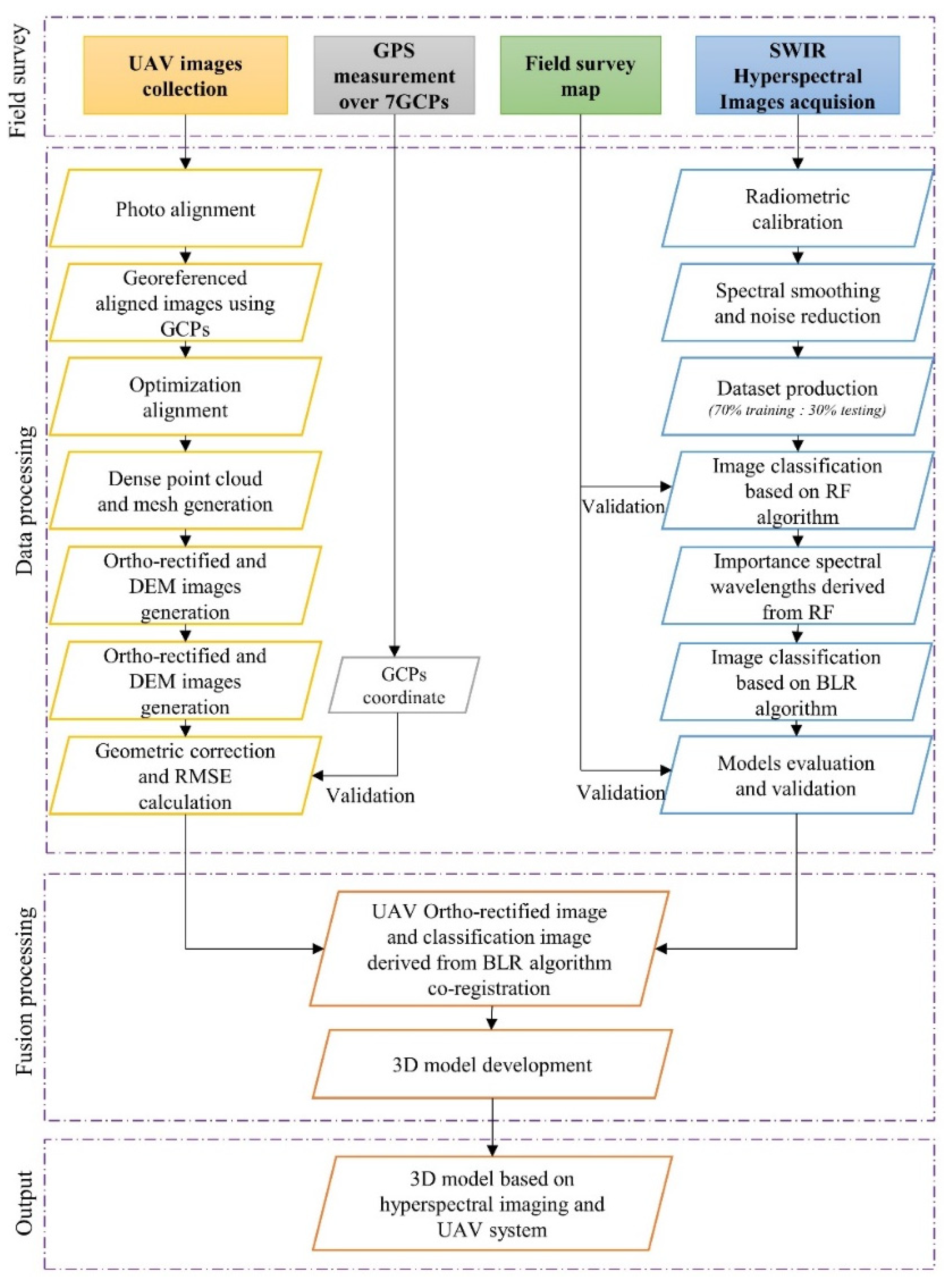
2. Materials and Methods
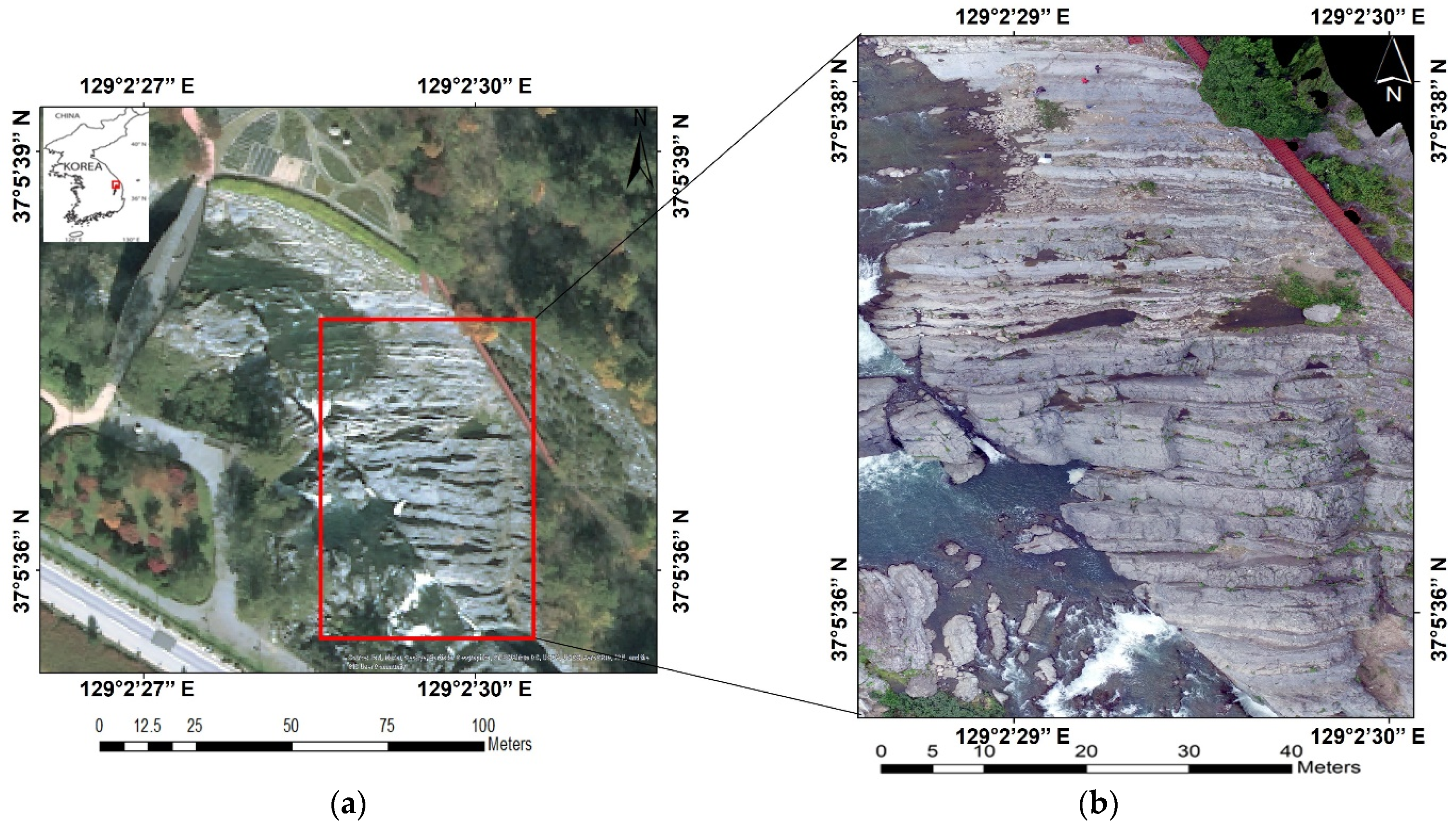
2.1. Study Area

The study area, Gumunso is in Taebaek city, Gangwon province (37°5′38″N and 129°2′29″E), 195 km east from Seoul in South Korea (Figure 1). The target outcrop has an area of 1881 square meters and exposed as a rocky outcrop along a stream. The outcrop shows an alternative rock formation between limestone and dolostone with a dimension of 22 by 42 m. The outcrop belongs to Makgol formation consisting of dominant lithofacies of dark gray massive dolostone, sometimes intercalated with bioturbated wackestone/grainstone and limestone conglomerate [16,17,18,19]. The Makgol formation is characterized by cyclic sedimentation of meter-scale shallowing-upward units in a peritidal environment in the latter part of the Paleozoic era [20]. Due to the stratigraphic distribution with topographic variation, the study site is ideal for developing a 3D integrative geologic model using hyperspectral imaging analysis and a UAV-based 3D surface model.

2.2. Hyperspectral Image Acquisition and Preprocessing

The study outcrop was scanned by a HySpex SWIR–384 SWIR hyperspectral camera in 288 spectral channels, ranging from 930 to 2500 nm (Table 1). For field operations, to ensure stable and reliable acquisition of images on a corrugated surface, a rugged yet portable tripod was used. Barium sulfate white and black reference panels were stationed in the field of view for radiometric calibration. The images were acquired from 14:00 to 17:30 on 28 May 2020, under a natural illumination condition with sufficient incident energy to ensure a continuous spectrum captured by the camera. Then, the integration time and the camera focus were adjusted for preferable image acquisition. After adjusting these presets, the hyperspectral image was referenced to panels followed by outcrop scanning [21]. The target outcrop was scanned 6 times for 2 sections at 60 m distance from the target for maximum image coverage. After radiometric calibration, we selected the two best hyperspectral images (1616 × 620 pixels) for further analysis (Figure 2).
The SWIR hyperspectral images were smoothed by the Savitsky-Golay smoothing filter to remove noisy signals [22]. After that, dark subtraction and minimum noise fraction (MNF) transformation were applied to remove random noise and correct atmospheric noise in the images. The MNF transformation is composed of two cascaded principal component transformations (PCT). The first PCT uses the sampled noise covariance to transform noise to white noise (unit variance and no band-to-band correlation). The second PCT transforms the noise-whitened data to two parts: large eigenvalues corresponding to coherent images and near-unity eigenvalues corresponding to noise dominated images. The noise dominated images were treated by low-pass filters to suppress the noise. A backward transform was performed to restore the spectral bands with minimal noise content [23,24]. The noise-reduced hyperspectral images were used for further analyses [25]. The image pro-processing and further imaging analysis were conducted by ENVI (Harris Geospatial, Boulder, CO, USA) and Rstudio (Integrated Development for R. RStudio, PBC, Boston, MA, USA).

2.3. UAV Survey and DEM Processing

This study selected seven ground control points (GCP hereafter) over the UAV survey site for geometric calibration and accuracy assessment of the output orthorectified image and DEM. To avoid bias in geometric correction, the positions of GCPs were uniformly spread over the study area (Figure 3). The location of GCPs were measured by Trimble R2 GNSS Receiver based on the virtual reference station (VRS) system with max horizontal accuracy of 10 mm and vertical accuracy of 20 mm.
This study used DJI’s Phantom 4 Pro+ UAV to obtain an orthorectified image and DEM. The UAV data was acquired simultaneously with hyperspectral scanning in a sunny weather condition with no cloud cover. Over 100 UAV images were acquired at an altitude of 40 m with 65% overlap at image resolution of 4000 × 3000 pixels. Point clouds were extracted from the UAV images by the SfM algorithm using Agisoft PhotoScan software [26,27]. The UAV data processing for construction of orthorectified image and digital elevation model (DEM) was carried out by the procedure in Figure 4.

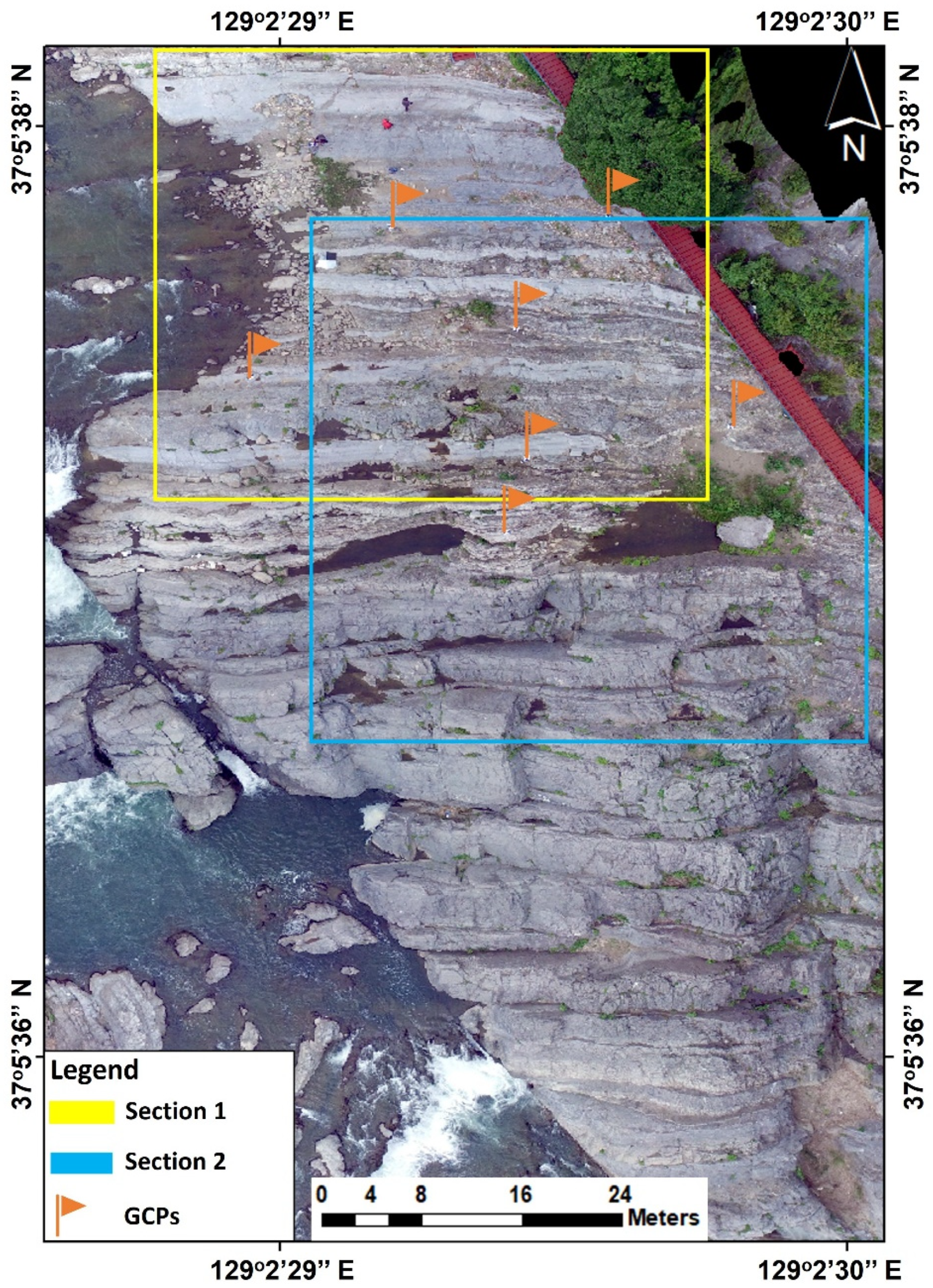
2.4. Ground Truthing of the Outcrop

Ground truth data were obtained by field inspections and air-photo delineation in a GIS environment. The field survey was conducted at the same date of the hyperspectral and UAV data acquisition. Each rock layer was inspected by a field geologist about lithology, and the geometric properties including thickness, strike and dip of each rock layer were measured. Microscopic observation of rock layers was additionally carried out for definition of rock layers composing the out crop. The field survey map was, then, reinterpreted to the UAV air-photo to be used as ground truth data to train and validate the hyperspectral image classification (Figure 3).

2.5. Spectral Analysis

In the shortwave infrared wavelength region, many mineral groups have distinct absorption features caused by their chemical component. For instance, the spectral characteristics of carbonate rocks such as limestone and dolostone have distinctive absorption features at 2340–2345 and 2320–2328 nm due to CO32− ion [28]. These spectral features can be used to distinguish calcite, dolomite, and other non-carbonate minerals [29]. The absorption feature at 2300–2350 nm is the most noticeable for carbonate rocks when using ground-based Hyperspectral Camera under natural illumination [30].
This study analyzed the spectral characteristics of rock formations in the target outcrop based on pre-processed reflectance spectra and hull quotient corrected spectra extracted from the hyperspectral image pixels. The hull quotient correction technique maximizes and characterizes absorption features, and, thus, is useful for detecting the position and absorption depth characteristics [31].

2.6. Band Selection and Spectral Index Derivation

The random forest (RF) classification algorithm was applied to the preprocessed hyperspectral images to select the most effective bands to distinguish different carbonate rock types. Although RF can provide accurate classification results, the extendibility of such model is questionable: the model trained in one study site cannot be used in others. Therefore, the purpose of using random forest is to use the Gini index provided by the RF model as a guidance to build a more straightforward logistic regression model with better extendibility. The training and validation pixels were randomly selected from the hyperspectral image based on the field survey data. In total, 70% of the extracted image pixels (24,198 pixels) were used as training data for RF model development, and the remaining 30% of pixels (10,370 pixels) were used for validation of the classification model. Moreover, 482 mineral and 76 rock spectra from USGS and JPL spectral libraries were included for RF and spectral indices development to identify spectral variables effective to distinguish limestone and dolostone from commonly found rocks and minerals. The mineral spectra include rock forming minerals, a total of 482 mineral spectra and 76 rock spectra. The library mineral spectra include hydrothermal alteration minerals and ore minerals, which are considered the most possible mineral occurrences including alunite, beryl, biotite, calcite, dolomite, chlorite, epidote, fluorite, gypsum, kaolinite, muscovite, pyrophyllite, quartz, tourmaline, and so on. The library rock spectra also include common rock occurrences in the field such as pyroxenite, gneiss, gabbro, sandstone, marble, basalt, limestone, dolostone, shale, granite, diorite, pegmatite, diabase and so on.
RF is a classification algorithm based on decision trees and improved bagging and bootstrapping techniques [32]. The bagging and bootstrapping selected 2/3 samples for training a tree each time and reserved 1/3 samples as out of bag (OOB) validation. Trees were generated by repeating randomized formation of sample and variable sets using the bagging and bootstrapping strategy [33,34,35]. Classification decisions are made by major votes from the trees. The two parameters to be specified in RF classification algorithm are ntree (number of trees to grow) and mtry (number of variables to divide at each node). The RF algorithm selects important bands based on the variable importance by the mean decrease Gini (data purity). The lower the Gini index, the more important the variable in the classification model [36]. We analyzed the spectral bands most useful for the rock classification and used them for further model development. The RF classification was assessed with the overall accuracy, kappa coefficient, commission and omission errors compared to the field survey map [37].
To derive the indices for detection of carbonate rocks including limestone and dolostone for field application, this study used binary logistic regression (BLR). The BLR is composed of one or multiple independent variables that describe a relationship to a dependent response variable [38,39]. In this study, the limestone or dolostone occurrence (variable Y) is regulated by the spectral value of specific bands (variable X) and used to predict an event occurring with only 2 numbers indicating limestone (1) and non-limestone (0) and dolostone (1) and non-dolostone (0). We derived a binary logistic regression equation with probability value of 0 or 1 based on the standard cutoff of 0.5. The equation can be written as a function of P as follows (1) [40,41,42].
P limestone   or   dolostone = e ( C + β 1 x 1 + β 2 x 2 + + β n x n ) 1 + e ( C + β 1 x 1 + β 2 x 2 + + β n x n )
where Plimestone or dolostone is the probability of limestone or dolostone occurrence, C is the constant (or intercept) of the equation, β is the coefficient (or beta weight) of the predictor variables and x is the reflectance value of the selected bandn.
Evaluation of the indices was based on the results of Hosmer and Lemeshow test, the Wald statistic, and pseudo-R2 values of “Nagelkerke” and “Cox and Snell”. The Hosmer-Lemeshow test is a Goodness-of-Fit test for logistic regression, especially for models of risk prediction. This test divides the samples to deciles (10-fold) and assesses the model performance in each subgroup by the probability of matching between observed and predicted values. Then, the Hosmer and Lemeshow statistic H is computed [36] with a p-value to evaluate if the logistic regression model made good predictions.
Furthermore, Cox-Snell and Nagelkerke R2 statistics were used to evaluate the BLR models, following Equations (2) and (3) below [43,44,45].
R 2 = 1 { L ( M Intercrpt ) L ( M Full ) } 2 N ,   Cox   and   Snell
R 2 = 1 { L ( M Intercrpt ) L ( M Full ) } 2 N 1 L ( M Intercrpt ) 2 N ,   Nagelkerke
where L(MIntercrpt) is the log-likelihood of the null model and L(MFull) is the log-likelihood of the full model. The ratio of the pseudo-R2 closer to 1 indicates the model has more potency [46]. Finally, the best equation for carbonate rock prediction was selected with the highest prediction accuracy.

2.7. Fusion of Hyperspectral Imaging and UAV-Based 3D Model

The integrative 3D geologic model for carbonate rocks was constructed using Autodesk 3ds Max (Autodesk, Inc., San Rafael, CA, USA) software based on the scale-invariant feature transform (SIFT hereafter) algorithm to find key-points between two images [47]. The key-points are conjugate points easily recognizable between the classification map and the orthorectified image where geometric properties including coordinate, scale, and orientation were extracted for each key-point. The SIFT algorithm analyzed geometric properties of each key-point based on a 128-dimensional eigenvector (SIFT descriptor) and extracted SIFT descriptors for orthorectified image and the rock type map. Finally, the SIFT algorithm compared between SIFT descriptors of the orthorectified mosaic image and the rock type map to identify the best matching coefficients for image co-registration [48,49]. Once the coordinates are matched, the classified rock type image is draped on the 3D surface of the rock to compute the geometric measures of the stratifications such as thickness, strike, dip, slope, and aspect.

3. Results and Discussion

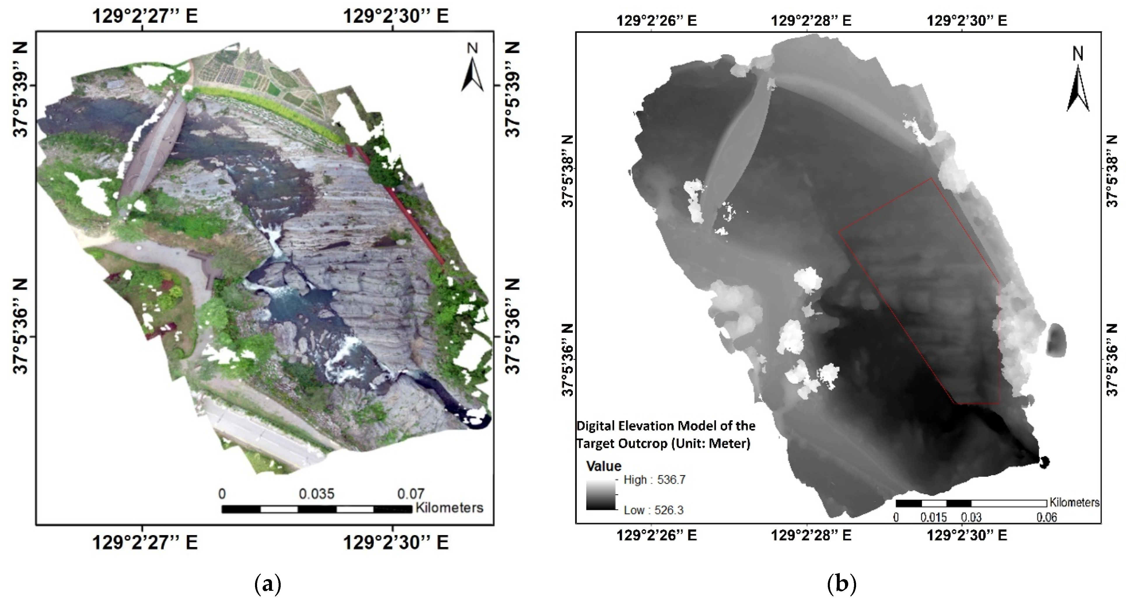
3.1. UAV-Based Orthorectified Image and Digital Elevation Model of the Outcrop

The UAV survey on the target outcrop constructed an orthorectified image at a spatial resolution of 1.7 cm with 7360 × 8448 pixels. The accuracy of orthorectified was assessed based on the GPS survey results of 7 GCPs. The overall RMSE of the orthorectified image was 21.1 cm. The orthorectified image revealed that the target outcrop has geometric properties of 228 m and 2175 m2 for perimeter and area, respectively (Figure 5a). Notably, the outcrop showed an alternative rock formation between two different types of lithology with colors ranging from white gray to dark gray.
The DEM derived from the UAV survey had a spatial resolution of 9 cm at 2828 × 2990 pixels. In general, the overall horizontal and vertical RMSEs of the DEM image were 21.1 and 37.4 cm. The derived DEM revealed that the target outcrop (marked with red square) is topographically positioned at a minimum elevation of 526.3 m to a maximum elevation of 536.7 with the slope of the target outcrop surface ranging from 36 to 58 degrees to the South (Figure 5b).

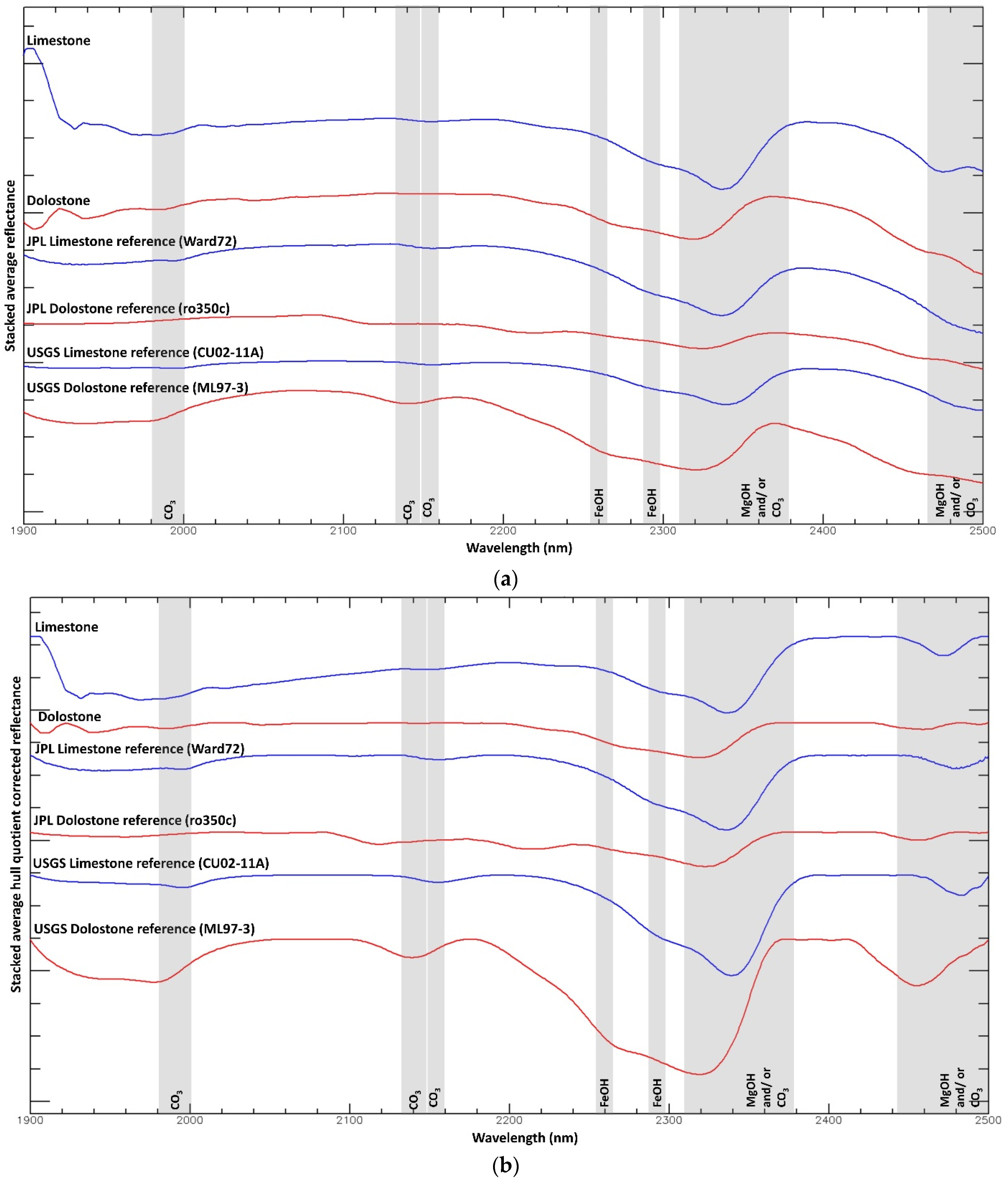
3.2. Spectral Characteristics of Limestone and Dolostone

The spectral characteristics of carbonate rocks forming the target outcrop were analyzed based on reflectance and hull quotient spectra. From the previous studies, the average surface reflectance of carbonate rocks in the outcrop when using ground-based Hyperspectral Camera under natural illumination can observe from 2000 to 2400 nm wavelength range, because other spectral regions are blurred and degraded by strong atmospheric scattering [5,9,28]. The occurrence of the carbonate rocks in the study area could be recognized from the weak absorption features at 2140 nm for the dolostone and 2150 nm for the limestone manifested by CO32− ion (Figure 6) [50]. The limestone shows additional absorption features around 1990, 2150, 2295, 2340 and 2480 nm, where the strongest absorption features at 2340 nm and minor absorptions at 1990, 2150, and 2480 nm are manifested by CO32− ion of calcite and that at 2295 nm is associated with FeOH (Figure 6). The spectral characteristics of the target limestone coincides well with the reference spectra of limestone and calcite (Figure 6) except the FeOH absorption. Given that FeOH absorption is mainly associated with clay minerals, it indicates that the limestone of the target outcrop is mainly composed of calcium carbonate mineral (calcite) with minor content of clay minerals. The hull quotient corrected spectra of limestone in the target outcrop shows strong absorption features at 2340 nm followed by 2480 nm where the absorption features were identical to the library references of limestone (Figure 6b) confirming the calcite as major mineral component.
The absorption features of dolostone in the target outcrop are at 1990, 2140, 2260, 2320 and 2470 nm, where absorptions at 1990, 2140, 2320 and 2470 nm are manifested by Mg and CO32− component, and that at 2260 nm is associated with FeOH (Figure 6). The distinctive differences between the limestone and dolostone in the target outcrop can be detected at their absorption features. Limestone in the target outcrop shows strong absorption at 2340 nm while dolostone shows weaker absorption at 2320 nm which shifted toward shorter wavelengths. This phenomenon is a characteristic spectral behavior between calcite and limestone reported by previous studies [5,9,10,11,50,51]. The spectral characteristics of the target dolostone coincides well with the reference spectra of dolomite and dolostone (Figure 6), while the absorption depth of target dolostone is relatively weaker. It indicates that the target dolostone is not a pure dolostone but contains clay minerals as accessary minerals [52].

3.3. Carbonate Rock Classification

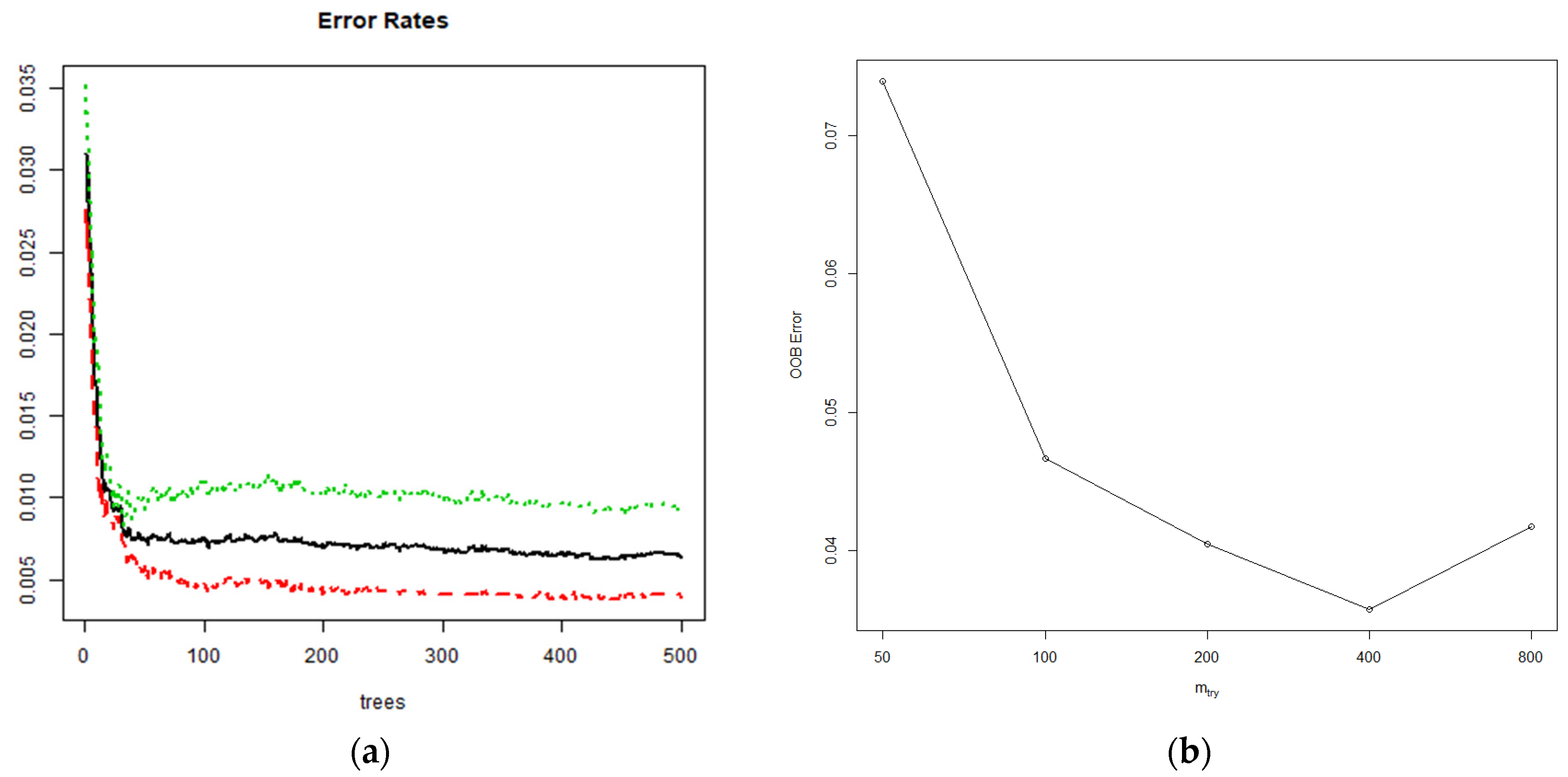
3.3.1. Carbonate Rock Classification by Random Forest Classification

A total of 34,569 pixels of the hyperspectral images were extracted from limestone and dolostone in the target outcrop for training and validation data of the RF and BLR algorithms. For each classification algorithm, the dataset was randomly partitioned into 70% to train the model and the remaining 30% for validation. Based on the training data, the classification map of limestone and dolostone was derived by RF classification from the SWIR hyperspectral images. In this study, we set the ntree value to 250 trees and mtry to 400 based on the OOB error analysis (Figure 7).
The accuracy assessment of the classification on limestone and dolostone showed high overall accuracy and kappa coefficient of 91.71% and 0.89, respectively (Table 2). The RF algorithm showed good performance for carbonate rock classification in the target outcrop with high overall accuracy, kappa coefficient, and low commission and omission errors for both training and validation data (Table 2).

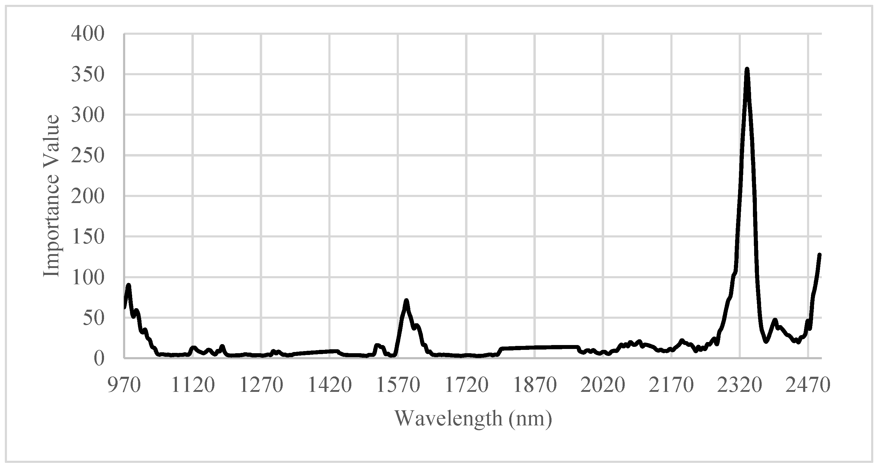
3.3.2. Band Selection and Derivation of Carbonate Rock Indices from Binary Logistic Regression

The variable importance plot shows the most important variables marked at the wavelength from 2300 to 2362 nm followed by 2450–2495 nm, 970–1026 nm and 1548–1656 nm (Figure 8). The first tier is the major absorption features of limestone and dolostone from 2320 to 2345 nm manifested by MgOH and/or CO32−. In particular, the peak importance occurs at 2336 nm where absorption features of 70% pure calcite are found [9], followed by a second peak at 2341 nm manifested of CO32− ion. The third peak is at 2331 nm related to MgOH and/or CO32−. The second tier is the absorption features of limestone and dolostone from 2450 to 2495 nm. The third and the last tiers are from 970 to 1026 nm and 1548 to 1656 nm related to absorption features of clay minerals. Through the RF’s variable importance index, 30 bands were selected because they also gave the lowest OOB errors [11]. These 30 bands were used to construct the BLR models.
The spectral indices for detection of carbonate rocks derived by BLR model showed that the best detection model of limestone was the one using 15 spectral bands associated with OH, AlOH, FeOH, MgOH and/or CO32− absorption features, among which the MgOH and/or CO32− absorptions are associated with eight bands (Table 3). Different from limestone, the dolostone model was developed based on nine spectral bands associated with three bands at MgOH and/or CO32− absorptions and six bands of clay minerals (Table 3).
Both models are statistically significant in the Pseudo-R2 goodness of fit test 0.734 and 0.979 for limestone, and 0.712 and 0.956 for dolostone. Generally, Cox and Snell pseudo-R2 values higher than 0.2 are a meaningful fit [53]. The results of the Hosmer and Lemeshow test showed that p values of the BLR model were 0.662 for limestone and 0.07 for dolostone. In the Hosmer and Lemeshow test, the p value higher than 0.05 cannot reject the null hypothesis, which indicates the model is acceptable [54] (Table 4).
Accuracy assessment of validation data showed an overall accuracy of 87.91% and a kappa coefficient of 0.77 (Table 5). It indicates that these models can distinguish limestone and dolostone with high accuracy and acceptable statistical significance. Compared to the RF model, although the accuracy of the BLR models is lower than the RF model, they are more generalizable because there are only several coefficients to be adjusted rather than the complex decision making structure of the RF model. Furthermore, the detection model in this study also included various rocks and mineral spectra commonly found in geological units. Therefore, the detection model derived by BLR is easier to interpret for geological survey.
Chung et al. [10] also suggested important variables to detect magnesite and associated gangue minerals, where they used 14 spectral bands for dolomite detection based on nine spectral bands associated with MgOH features, four bands of Ca features and another band at 1248 nm. For calcite detection, 15 spectral bands were derived based on nine wavelengths from MgOH features, with another four bands from Ca features and the bands at 1237 and 1248 nm. Compared to the previous study, our study also found 15 spectral bands for limestone detection at 980, 1584, 2290, 2295, 2300, 2306, 2316, 2321, 2331, 2336, 2341, 2346, 2352, 2362 and 2480 nm and nine spectral bands for dolostone detection at 1968, 2009, 2024, 2055, 2091, 2132, 2300, 2336 and 2341 nm based on MgOH, CO32− and clay mineral absorption features (Table 3 and Figure 6). The model accuracy using field data is as good as laboratory samples, which is a generalization example of laboratory experiments to real-world cases.

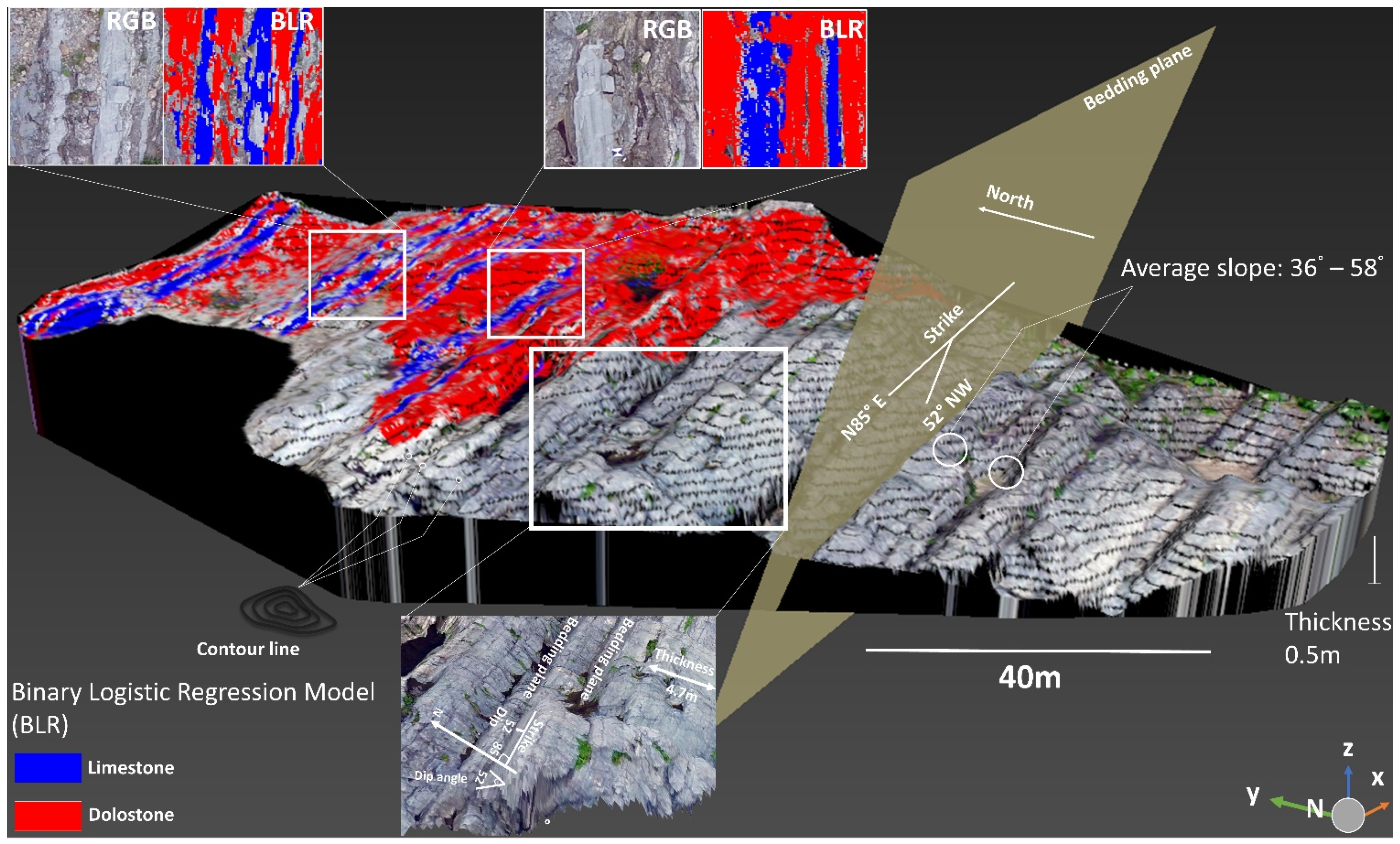
3.4. Fusion of Classification Map and UAV-Based 3D Model

The co-registration between HIS and UAV images ensures the match up of the BLR result with the rasterized DEM from the UAV image point cloud. The integration between BLR image and the DEM was completed by draping the BLR image on the DEM. The geometric properties were then computed from the DEM. As lithology is extracted from hyperspectral images, the 3D model shows the position of the extracted sedimentary rock layers as well as bedding planes (Figure 9). The 3D coordinates (x, y, z) of the elements in the rock layer map can be used to calculate 3D geometric properties of the layers such as strike and dip, where strike is the azimuthal direction of a bedding plane, and dip is the slope angle of it (Figure 9). The rock layer thickness ranges from 0.4 to 4.7 m, which matches with field survey results. Furthermore, our 3D model revealed that the strike and dip of the rock layers are N85°E and 52°NW (Figure 9). The geological and topographic information extracted from the model was verified by the field survey data. The results suggest that our approach using HIS and UAV data can obtain reliable measurements of rock layer thickness, strike, and dip for understanding geological positioning of different rock layers, geological profile, and geological relationship between rock layers without contact surveys.
One limitation found by this case study is that because of the roughness of the rock, it was difficult to find an ideal illumination condition to cover the entire rock body during one time of survey (Figure 9). There were always shadows on the rock surface, which must be removed from the classification. The 3D point cloud was also degraded by the shadows because the SfM algorithm relies on image matching between features excluding shadows. Therefore, multiple trips are needed to obtain a shadow-free, full coverage of the rock outcrop, and there would be another problem of dealing with the changing illumination conditions.

4. Conclusions

This work introduced an integrative 3D model between hyperspectral mapping and a UAV-based 3D model for a carbonate rock outcrop. A carbonate rock outcrop composed of alternative layers of limestone and dolostone was scanned with a SWIR hyperspectral imaging system and classified with an RF algorithm to derive spectral bands sensitive to mapping of carbonate rocks for constructing logistic regression models. A DEM and ortho-rectified images were generated by the SfM algorithm from UAV images. The hyperspectral classification map was co-registered with the ortho-rectified image using the best-matching SIFT descriptor pairs as control points, and the integrative 3D geologic model was developed.
The spectral characteristics of limestone and dolostone showed variations in MgOH and CO32− absorption features. The spectral analysis revealed that the target limestone is relatively purer than dolostone as dolostone has weaker absorption of dolomite with weak clay absorptions. The RF classification achieved an overall accuracy of 91.71% and a kappa coefficient of 0.89. As an outcome, 30 bands with the highest Gini index from the RF model were extracted from OH, AlOH, FeOH, MgOH and CO32− absorption features. The logistic regressions using the spectral indices had an overall accuracy of 87.73% for limestone and 88.02% for dolostone. Given that the spectral indices were derived from field data with consideration of commonly found geological materials, the indices have better applicability in the real-world cases than laboratory samples.
Using the 3D mineral map produced by draping the mineral classification result on the UAV digital surface model, detailed measurement of lithologic units such as rock type, thickness, strike, and dip were extracted from the model. Therefore, the method introduced in this study opens a fast, reliable, and convenient option for geological surveys, and provides a fast, convenient solution to expediting geological surveys. Furthermore, the model can be easily extended for a subsurface geological model and mineral resources assessment.

Author Contributions

Conceptualization, J.Y. and H.H.H.; methodology, J.Y., H.H.H. and L.W.; software, H.H.H.; validation, J.Y., S.C. and H.H.H.; formal analysis, H.H.H.; investigation, J.Y., H.H.H. and L.W.; resources, N.H.K. and B.H.L.; data curation, H.H.H. and J.Y.; writing—original draft preparation, H.H.H. and J.Y.; writing—review and editing, J.Y., L.W. and T.H.P.; visualization, H.H.H. and J.Y.; supervision, J.Y.; project administration, B.H.L. and S.-M.K.; funding acquisition, S.-M.K. All authors have read and agreed to the published version of the manuscript.

Funding

This work was supported by the National Research Council of Science and Technology (NST) grant by the Korea Government (MSIT) (No. CRC-15-06-KIGAM) and the National Research Foundation (NRF) of Korea grant by the Korean Government (NRF-2020R1A2C2005439).

Institutional Review Board Statement

Not applicable.

Informed Consent Statement

Not applicable.

Acknowledgments

The authors deeply appreciate anonymous academic editor and reviewers for their constructive comments.

Conflicts of Interest

The authors declare no conflict of interest.

References

  1. Blatt, H.; Jones, R.L. Proportions of Exposed Igneous, Metamorphic, and Sedimentary Rocks. GSA Bull. 1975, 86, 1085. [Google Scholar] [CrossRef]
  2. Blatt, H.; Middleton, G.; Murray, R. Origin of Limestones. In Origin of Sedimentary Rocks; Prentice-Hall: Englewood Cliffs, NJ, USA, 1972; pp. 409–455. [Google Scholar]
  3. Pettijohn, F.J. Limestones and Dolomite. In Sedimentary Rocks, 3rd ed.; Harper & Row: New York, NY, USA, 1975; pp. 316–391. [Google Scholar]
  4. Best, M.; Ku, T.; Kidwell, S.; Walter, L. Carbonate Preservation in Shallow Marine Environments: Unexpected Role of Tropical Siliciclastics. J. Geol. 2007, 115, 437–456. [Google Scholar] [CrossRef] [Green Version]
  5. Zaini, N.; Van der Meer, F.; Van der Werff, H. Determination of Carbonate Rock Chemistry Using Laboratory-Based Hyperspectral Imagery. Remote Sens. 2014, 6, 4149–4172. [Google Scholar] [CrossRef] [Green Version]
  6. Dalm, M.; Buxton, M.W.N.; Van Ruitenbeek, F.J.A. Discriminating ore and waste in a porphyry copper deposit using short-wavelength infrared (SWIR) hyperspectral imagery. Miner. Eng. 2017, 105, 10–18. [Google Scholar] [CrossRef]
  7. Buddenbaum, H.; Steffens, M. The Effects of Spectral Pretreatments on Chemometric Analyses of Soil Profiles Using Laboratory Imaging Spectroscopy. Appl. Environ. Soil Sci. 2012, 2012, 274903. [Google Scholar] [CrossRef] [Green Version]
  8. Speta, M.; Rivard, B.; Feng, J.; Lipsett, M.; Gingras, M. Hyperspectral imaging for the determination of bitumen content in Athabasca oil sands core samples. AAPG Bull. 2015, 99, 1245–1259. [Google Scholar] [CrossRef]
  9. Lorenz, S.; Salehi, S.; Kirsch, M.; Zimmermann, R.; Unger, G.; Vest Sørensen, E.; Gloaguen, R. Radiometric Correction and 3D Integration of Long-Range Ground-Based Hyperspectral Imagery for Mineral Exploration of Vertical Outcrops. Remote Sens. 2018, 10, 176. [Google Scholar] [CrossRef] [Green Version]
  10. Chung, B.; Yu, J.; Wang, L.; Kim, N.H.; Lee, B.H.; Koh, S.; Lee, S. Detection of Magnesite and Associated Gangue Minerals using Hyperspectral Remote Sensing—A Laboratory Approach. Remote Sens. 2020, 12, 1325. [Google Scholar] [CrossRef] [Green Version]
  11. Kirsch, M.; Lorenz, S.; Zimmermann, R.; Tusa, L.; Möckel, R.; Hödl, P.; Booysen, R.; Khodadadzadeh, M.; Gloaguen, R. Integration of Terrestrial and Drone-Borne Hyperspectral and Photogrammetric Sensing Methods for Exploration Mapping and Mining Monitoring. Remote Sens. 2018, 10, 1366. [Google Scholar] [CrossRef] [Green Version]
  12. Krupnik, D.; Khan, S.D. High-Resolution Hyperspectral Mineral Mapping: Case Studies in the Edwards Limestone, Texas, USA and Sulfide-Rich Quartz Veins from the Ladakh Batholith, Northern Pakistan. Minerals 2020, 10, 967. [Google Scholar] [CrossRef]
  13. Krupnik, D.; Khan, S.; Okyay, U.; Hartzell, P.; Zhou, H.-W. Study of Upper Albian rudist buildups in the Edwards Formation using ground-based hyperspectral imaging and terrestrial laser scanning. Sediment. Geol. 2016, 345, 154–167. [Google Scholar] [CrossRef] [Green Version]
  14. Rokhmana, C.A. The Potential of UAV-based Remote Sensing for Supporting Precision Agriculture in Indonesia. Procedia Environ. Sci. 2015, 24, 245–253. [Google Scholar] [CrossRef] [Green Version]
  15. Teodoro, A.; Santos, P.; Espinha Marques, J.; Ribeiro, J.; Mansilha, C.; Melo, A.; Duarte, L.; Rodrigues de Almeida, C.; Flores, D. An Integrated Multi-Approach to Environmental Monitoring of a Self-Burning Coal Waste Pile: The São Pedro da Cova Mine (Porto, Portugal) Study Case. Environments 2021, 8, 48. [Google Scholar] [CrossRef]
  16. Byun, U.H.; Lee, H.S.; Kwon, Y.K. Sequence stratigraphy in the middle Ordovician shale successions, mid-east Korea: Stratigraphic variations and preservation potential of organic matter within a sequence stratigraphic framework. J. Asian Earth Sci. 2018, 152, 116–131. [Google Scholar] [CrossRef]
  17. Kwon, Y.; Chough, S.; Choi, D.; Lee, D. Sequence stratigraphy of the Taebaek Group (Cambrian–Ordovician), mideast Korea. Sediment. Geol. 2006, 192, 19–55. [Google Scholar] [CrossRef]
  18. Choi, D.K.; Chough, S.K. The Cambrian-Ordovician stratigraphy of the Taebaeksan Basin, Korea: A review. Geosci. J. 2005, 9, 187–214. [Google Scholar] [CrossRef]
  19. Chough, S.K.; Kwon, S.T.; Ree, J.H.; Choi, D.K. Tectonic and sedimentary evolution of the Korean Peninsula: A review and new view. Earth-Sci. Rev. 2000, 52, 175–235. [Google Scholar] [CrossRef]
  20. Woo, K.S. Cyclic tidal successions of the Middle Ordovician Maggol Formation in the Taebaeg area, Kangwondo, Korea. Geosci. J. 1999, 3, 123–140. [Google Scholar] [CrossRef]
  21. Behmann, J.; Acebron, K.; Emin, D.; Bennertz, S.; Matsubara, S.; Thomas, S.; Bohnenkamp, D.; Kuska, M.T.; Jussila, J.; Salo, H.; et al. Specim IQ: Evaluation of a New, Miniaturized Handheld Hyperspectral Camera and Its Application for Plant Phenotyping and Disease Detection. Sensors 2018, 18, 441. [Google Scholar] [CrossRef] [Green Version]
  22. Tsai, F.; Philpot, W. Derivative Analysis of Hyperspectral Data. Remote. Sens. Environ. 1998, 66, 41–51. [Google Scholar] [CrossRef]
  23. Green, A.; Berman, M.; Switzer, P.; Craig, M. A transformation for ordering multispectral data in terms of image quality with implications for noise removal. IEEE Trans. Geosci. Remote. Sens. 1988, 26, 65–74. [Google Scholar] [CrossRef] [Green Version]
  24. Dabiri, Z.; Lang, S. Comparison of Independent Component Analysis, Principal Component Analysis, and Minimum Noise Fraction Transformation for Tree Species Classification Using APEX Hyperspectral Imagery. ISPRS Int. J. Geo-Inf. 2018, 7, 488. [Google Scholar] [CrossRef] [Green Version]
  25. Kennedy, R.E.; Townsend, P.; Gross, J.E.; Cohen, W.B.; Bolstad, P.; Wang, Y.; Adams, P. Remote sensing change detection tools for natural resource managers: Understanding concepts and tradeoffs in the design of landscape monitoring projects. Remote. Sens. Environ. 2009, 113, 1382–1396. [Google Scholar] [CrossRef]
  26. Moyano, J.; Nieto-Julián, J.E.; Antón, D.; Cabrera, E.; Bienvenido-Huertas, D.; Sánchez, N. Suitability Study of Structure-from-Motion for the Digitisation of Architectural (Heritage) Spaces to Apply Divergent Photograph Collection. Symmetry 2020, 12, 1981. [Google Scholar] [CrossRef]
  27. Cabrelles, M.; Lerma, J.L.; Villaverde, V. Macro Photogrammetry & Surface Features Extraction for Paleolithic Portable Art Documentation. Appl. Sci. 2020, 10, 6908. [Google Scholar] [CrossRef]
  28. Zaini, N.; Van der Meer, F.; Van der Werff, H. Effect of Grain Size and Mineral Mixing on Carbonate Absorption Features in the SWIR and TIR Wavelength Regions. Remote Sens. 2012, 4, 987–1003. [Google Scholar] [CrossRef] [Green Version]
  29. Clark, R.N.; Swayze, G.A.; Wise, R.; Livo, E.; Hoefen, T.; Kokaly, R.; Sutley, S.J. USGS Digital Spectral Library splib06a: U.S. Geological Survey, Digital Data Series 231. 2007. Available online: https://www.usgs.gov/labs/spec-lab/capabilities/superseded-spectral-library-versions?qt-capabilities_objects=0#qt-capabilities_objects (accessed on 30 April 2021).
  30. Kaab, A. Remote Sensing of Mountain Glaciers and Permafrost Creep; Geographisches Institut der Universität Zürich: Zurich, Switzerland, 2005; 264p. [Google Scholar]
  31. Kokaly, R.F.; Clark, R.N. Spectroscopic Determination of Leaf Biochemistry Using Band-Depth Analysis of Absorption Features and Stepwise Multiple Linear Regression. Remote Sens. Environ. 1999, 67, 267–287. [Google Scholar] [CrossRef]
  32. Efron, B. Bootstrap Methods: Another look at the Jackknife. Ann. Stat. 1979, 7, 1–26. [Google Scholar] [CrossRef]
  33. Breiman, L.; Cutler, A. Random Forests—Classification Manual. Available online: http://www.math.usu.edu/~adele/forests/ (accessed on 30 April 2021).
  34. Breiman, L. Random Forests. Mach. Learn. J. Pap. 2001, 45, 5–32. [Google Scholar] [CrossRef] [Green Version]
  35. Lawrence, R.L.; Wood, S.D.; Sheley, R.L. Mapping invasive plants using hyperspectral imagery and Breiman Cutler classifications (Random Forest). Remote Sens. Environ. 2006, 100, 356–362. [Google Scholar] [CrossRef]
  36. Mellor, A.; Haywood, A.; Stone, C.; Jones, S. The Performance of Random Forests in an Operational Setting for Large Area Sclerophyll Forest Classification. Remote Sens. 2013, 5, 2838–2856. [Google Scholar] [CrossRef] [Green Version]
  37. Congalton, R.G.; Green, K. Assessing the Accuracy of Remotely Sensed Data: Principles and Practices, 3rd ed.; CRC Press Taylor Fr. Group: Boca Raton, FL, USA, 2019. [Google Scholar] [CrossRef]
  38. Davoudi Kakhki, F.; Freeman, S.A.; Mosher, G.A. Use of Logistic Regression to Identify Factors Influencing the Post-Incident State of Occupational Injuries in Agribusiness Operations. Appl. Sci. 2019, 9, 3449. [Google Scholar] [CrossRef] [Green Version]
  39. Borucka, A.; Grzelak, M. Application of Logistic Regression for Production Machinery Efficiency Evaluation. Appl. Sci. 2019, 9, 4770. [Google Scholar] [CrossRef] [Green Version]
  40. Štefko, R.; Horváthová, J.; Mokrišová, M. Bankruptcy Prediction with the Use of Data Envelopment Analysis: An Empirical Study of Slovak Businesses. J. Risk Financ. Manag. 2020, 13, 212. [Google Scholar] [CrossRef]
  41. Díaz-Pérez, M.; Carreño-Ortega, Á.; Gómez-Galán, M.; Callejón-Ferre, Á.-J. Marketability Probability Study of Cherry Tomato Cultivars Based on Logistic Regression Models. Agronomy 2018, 8, 176. [Google Scholar] [CrossRef] [Green Version]
  42. Hosmer, D.W., Jr.; Lemeshow, S.; Sturdivant, R.X. Applied Logistic Regression; John Wiley & Sons: New Jersey, NJ, USA, 2013; Volume 398. [Google Scholar]
  43. Menard, S. Coefficients of determination for multiple logistic regression analysis. Am. Stat. 2000, 54, 17–24. [Google Scholar]
  44. Nagelkerke, N.J. A note on a general definition of the coefficient of determination. Biometrika 1991, 78, 691–692. [Google Scholar] [CrossRef]
  45. Deng, C.; Zhang, X.; Li, Y.; Xiong, Q. Garch Model Test Using High-Frequency Data. Mathematics 2020, 8, 1922. [Google Scholar] [CrossRef]
  46. Zizi, Y.; Oudgou, M.; El Moudden, A. Determinants and Predictors of SMEs’ Financial Failure: A Logistic Regression Approach. Risks 2020, 8, 107. [Google Scholar] [CrossRef]
  47. Lowe, D.G. Object recognition from local scale-invariant features. In Proceedings of the Seventh IEEE International Conference on Computer Vision, Corfu, Greece, 20–25 September 1999; Volume 2, pp. 1150–1157. [Google Scholar] [CrossRef]
  48. Dong, Y.; Jiao, W.; Long, T.; Liu, L.; He, G.; Gong, C.; Guo, Y. Local Deep Descriptor for Remote Sensing Image Feature Matching. Remote Sens. 2019, 11, 430. [Google Scholar] [CrossRef] [Green Version]
  49. Chen, S.; Yuan, X.; Yuan, W.; Niu, J.; Xu, F.; Zhang, Y. Matching Multi-Sensor Remote Sensing Images via an Affinity Tensor. Remote Sens. 2018, 10, 1104. [Google Scholar] [CrossRef] [Green Version]
  50. Clark, R.N.; King, T.V.V.; Klejwa, M.; Swayze, G.A.; Vergo, N. High spectral resolution reflectance spectroscopy of minerals. J. Geophys. Res. 1990, 95, 12653–12680. [Google Scholar] [CrossRef] [Green Version]
  51. Gaffey, S.J. Spectral reflectance of carbonate minerals in the visible and near infrared (0.35–2.55 microns); calcite, aragonite, and dolomite. Am. Mineral. 1986, 71, 151–162. [Google Scholar]
  52. Baissa, R.; Labbassi, K.; Launeau, P.; Gaudin, A.; Ouajhain, B. Using HySpex SWIR-320m hyperspectral data for the identification and mapping of minerals in hand specimens of carbonate rocks from the Ankloute Formation (Agadir Basin, Western Morocco). J. Afr. Earth Sci. 2011, 61, 1–9. [Google Scholar] [CrossRef]
  53. Clark, W.; Hoskings, P. Statistical methods for geographers. In Clark Statistical Methods for Geographers; John Wiley and Sons: New York, NY, USA, 1986. [Google Scholar]
  54. Mokhtari, A.R. Hydrothermal alteration mapping through multivariate logistic regression analysis of lithogeochemical data. J. Geochem. Explor. 2014, 145, 207–212. [Google Scholar] [CrossRef]
Figure 1. Location map of the study area (a) and the survey zone is marked with red square field photograph in the study by UAV (b).
Remotesensing 13 03037 g001
Figure 2. Two main sections and GCP locations over the target outcrop for UAV survey.
Remotesensing 13 03037 g002
Figure 3. Field survey map overlaid on the ortho-rectified image for validation of the classification.
Remotesensing 13 03037 g003
Figure 4. Methodology diagram in this study.
Remotesensing 13 03037 g004
Figure 5. The orthorectified image (a) and DEM (b) of the target outcrop derived from UAV survey.
Remotesensing 13 03037 g005
Figure 6. Stacked average surface reflectance of limestone and dolostone of the target outcrop compared with library reference spectra (a) and the average hull quotient corrected reflectance spectra of limestone and dolostone compared with library reference spectra (b).
Remotesensing 13 03037 g006
Figure 7. Variation of OOB error of Ntrees (a) and variation of OOB error of Mtry (b).
Remotesensing 13 03037 g007
Figure 8. Gini importance of wavelength derived from the RF algorithm.
Remotesensing 13 03037 g008
Figure 9. Fusion of hyperspectral imaging derived from binary logistic regression model (BLR) overlain on RGB UAV-based 3D model showing lithological distribution and geological positioning of the rock layers.
Remotesensing 13 03037 g009
Table 1. The technical specification for HySpex SWIR–384.
Spectral range930–2500 nm
Spatial pixels384
Spectral channels288
Spectral sampling5.45 nm
FOV16°
Pixel FOV across/along0.73/0.73 mrad
Bit resolution16 bit
Noise floor150 e
Dynamic range7500
Peak SNR (at full resolution)>1100
Max speed400 fps
Power consumption30 W
Dimensions (l–w–h)38–12–17.5 cm
Weight5.7 kg
Table 2. Confusion matrix table of the training and validation data for the classification results from the RF algorithm.
ClassTraining Data
User’s
Accuracy
(%)
Producer’s
Accuracy
(%)
Commission
Error
(%)
Omission
Error
(%)
Limestone95.1295.514.884.49
Dolostone96.4195.173.594.83
Overall Accuracy: 95.34%
Kappa Coefficient: 0.91
ClassValidation Data
User’s
Accuracy
(%)
Producer’s
Accuracy
(%)
User’s
Accuracy
(%)
Omission
Error
(%)
Limestone93.592.386.57.62
Dolostone95.0491.034.968.97
Overall Accuracy: 91.71%
Kappa Coefficient: 0.89
Table 3. Selected wavelength for carbonate rock indices derived from BLR and Wald test results.
Wavelength (nm)β1S.E. 2Wald 3Df 4Sig. 5Exp (β) 6
Final selected spectral variables for limestone classification
9807.1260.72097.951101244.091
1584−0.0720.0870.69210.4060.930
2290−149.15860.0896.16210.0130
2295891.720187.40022.642100
2300−1737.397260.81744.374100
2306 nm1100.121164.15944.911100
2316 nm−468.074116.80516.058100
2321 nm902.109129.37548.620100
2331 nm−1073.833157.67746.381100
2336 nm1101.590217.57025.635100
2341 nm−1531.512301.27925.841100
2346 nm1627.802235.60747.734100
2352 nm−967.94895.835102.012100
2362 nm309.90027.601126.067100
2480 nm−19.5402.48162.014100
Constant−3.8370.344124.627100.22
Final selected spectral variables for dolostone classification
1968 nm−27.1846.08519.960100
2009 nm74.52914.97524.771100
2024 nm104.44720.91624.936100
2055 nm−417.08930.179191.004100
2091 nm173.93724.08452.157100
2132 nm40.5979.34418.877100
2300 nm−24.9354.79727.021100
2336 nm−458.28534.881172.621100
2341 nm537.31235.762225.745100
Constant−2.5120.245105.108100.081
β1 = logistic coefficient; S.E. 2 = standard error of estimate; Wald 3 = Wald chi-square values; df 4 = degree of freedom; Sig. 5 = p-value; Exp(B) 6 = exponentiated coefficient.
Table 4. The model summary of the BLR model in the target outcrop.
ParametersPseudo-R2Hosmer and Lemeshow Test
Cox and Snell R2Nagelkerke R2χ2dfp-Value
Limestone0.7340.9795.86980.662
Dolostone0.7120.95617.53380.07
Table 5. Confusion matrix table of the validation data for the classification results from the BLR algorithm.
ClassValidation Data
Overall Accuracy (%)Commission Error (%)Omission Error (%)
Limestone87.731.7712.27
Dolostone88.020.2211.98
Overall Accuracy: 87.91%
Kappa Coefficient: 0.77
Publisher’s Note: MDPI stays neutral with regard to jurisdictional claims in published maps and institutional affiliations.

