
Impervious Surfaces Mapping at City Scale by Fusion of Radar and Optical Data through a Random Forest Classifier


Department of Civil and Environmental Engineering and Construction, University of Nevada Las Vegas, Las Vegas, NV 89154, USA
*
Author to whom correspondence should be addressed.
Remote Sens. 2021, 13(15), 3040; https://0-doi-org.brum.beds.ac.uk/10.3390/rs13153040
Submission received: 10 June 2021
/
Revised: 29 July 2021
/
Accepted: 29 July 2021
/
Published: 3 August 2021
(This article belongs to the Special Issue Data Fusion for Urban Applications)
Abstract
:Urbanization increases the amount of impervious surfaces, making accurate information on spatial and temporal expansion trends essential; the challenge is to develop a cost- and labor-effective technique that is compatible with the assessment of multiple geographical locations in developing countries. Several studies have identified the potential of remote sensing and multiple source information in impervious surface quantification. Therefore, this study aims to fuse datasets from the Sentinel 1 and 2 Satellites to map the impervious surfaces of nine Pakistani cities and estimate their growth rates from 2016 to 2020 utilizing the random forest algorithm. All bands in the optical and radar images were resampled to 10 m resolution, projected to same coordinate system and geometrically aligned to stack into a single product. The models were then trained, and classifications were validated with land cover samples from Google Earth’s high-resolution images. Overall accuracies of classified maps ranged from 85% to 98% with the resultant quantities showing a strong linear relationship (R-squared value of 0.998) with the Copernicus Global Land Services data. There was up to 9% increase in accuracy and up to 12 % increase in kappa coefficient from the fused data with respect to optical alone. A McNemar test confirmed the superiority of fused data. Finally, the cities had growth rates ranging from 0.5% to 2.5%, with an average of 1.8%. The information obtained can alert urban planners and environmentalists to assess impervious surface impacts in the cities.
1. Introduction
By 2050, the world’s urban population is expected to nearly double, from 3.5 billion in 2010 [1]. Studies suggest that most of the growth will take place in developing countries, and cities may expand to as much as three times their sizes [2,3]. Urbanization brings forth the replacement of natural landscapes with built-up surfaces for accommodation [4,5,6,7]. Impervious surface knowledge is an important indicator of urbanization degree [8] as well as environmental quality [9]. The consequences of the surge in impervious cover include increases in the volume, duration, and intensity of surface runoff [10,11,12]; decreases of groundwater recharge [13,14,15,16,17,18,19,20]; and the degradation of receiving water sources, as they directly impact the flow of nonpoint source pollutants [21], which also affect the hydrologic cycle. Timely and accurate information on the changing land cover of developing cities will aid in decision making processes. This interests scientists, resources managers, and planners [22]. Such information can also benefit the development of Sustainable Development Goals (SDG Goal) targeted for the developing world by the United Nations. SDG Goal 11 aims to make cities safe, resilient, and sustainable, while SDG goal 6 aims to provide proper water supply and sanitation for all by 2030, demanding comprehensive knowledge of growth rates and expansion patterns of cities. The authors of [23] bring attention to the overwhelmed capacities of urban infrastructure such as water supply networks, solid waste management, and storm water drainage, due to lack of information on the expected amount of impervious surface and the corresponding surface runoff.
Both remotely sensed data and field measurements are used to quantify impervious surfaces. Ground truth acquisition, though reliable, is expensive and time consuming, especially for developing countries. Research in [24] highlights the popularity of satellite datasets in environmental studies with impervious-surface applications. Land use and land cover classification has advanced rapidly with remote sensing data [25,26,27,28,29,30,31].
Despite advances in space-borne sensors, limitations such as data not linking uniquely to land cover, and ambiguity with land uses persists. The authors’ data from [32] identified fusion as a promising tool, due to its ability to combine information on land properties from sensors operating with fundamentally different physical principles. They found 28 studies supporting improved results of fusion relative to single data source in their review. For example, the spectral reflectance and various indices (e.g., normalized difference built-up index (NDBI)) of built-up surfaces from several bands of optical sensor depend on the material. Similarly, microwave energy, scattered by those surfaces from radar sensor, depends on orientation and dielectric properties. Image fusion techniques can be distinguished into three categories based on their integration level: pixel level, feature level, and decision level. The first category comprises geocoding and co-registration to stack images’ pixels [33], while the second refers to each dataset’s feature extraction [34,35,36,37].
The European Space Agency (ESA) developed the Copernicus Mission, with a set of satellite families called Sentinel (S). S-1A and S-2A were launched on 3 April 2014, and 23 June 2015, respectively, followed by their twins (1B and 2B) on 25 April 2015 and 7 March 2017, respectively. Mapping of land surfaces is one of their applications. S-1 are active radar pairs, immune to weather conditions, while S-2 are passive optical satellites, with 13 bands [38]. Both satellite-based radar and optical data were constrained by low spatial and temporal coverage of medium resolution data in the past, which can be overcome with high spatial-, temporal-, and spectral-resolution S-1 and S-2 data [32]. The free and public data access policy of Sentinel data makes them more prospective for studying the additive value of data fusion.
While there are studies available for impervious surface mapping (ISM) of national, regional and provincial levels, studies focusing on spatiotemporal change at city scales are still scarce. A smaller spatial scale demands more attention to details as a city is full of dynamic land cover classes as there is a higher chance of mixed classes within a pixel. For comprehensive summary of impervious cover worldwide the following land cover dataset exists: MODIS Land Cover type product (annual 500 m resolution), GlobCover (GLC) 2009 (300 m resolution, 1 January 2009–1 January 2010), the China impervious fraction map (500 m resolution, 2000, 2005, 2010), and Copernicus Global Land Service (100 m resolution, annual from 2015–2019) (Copernicus Service Information). Such coarse temporal and spatial resolution render them inadequate for in depth analysis.
Conventional parametric statistical techniques, common with remote sensing, are not appropriate for classification [39]. Thus, more general ensemble classifiers are gaining attention, such as random forest (RF). They are known to have improved classification accuracy significantly [40]. Lighter computation and insensitivity to noise or overtraining with features to estimate the importance of each feature are some of its attractive characteristics.
Past studies have combined optical and radar data and utilized machine learning for land use land cover change assessment in cloud-prone regions [41], winter vegetation cover extraction [42], crop mapping [43,44], plastic-mulched landcover extraction [45], monitoring of tropical rainforest [46], monitoring wetlands [47], urban mapping [48], and change detection [49]. Land cover classification for various purposes such as flood mapping [50,51], agricultural landscapes [52], forest cover derivation [53] also took advantage of the fusion of S-1 and S-2 data. The authors of [54] developed various fusion strategies to combine different remote sensing data. They focused on improved discrimination power of remote sensing data due to additional information from SAR images, such as height of terrain. Such integration has proven improvement over optical data alone, with an increase in overall accuracy of up to 6% [41,42] and up to 13.5% [52]. There are not many studies emphasizing the extraction of man-made built-up surfaces for urban monitoring except with reference to filling in the temporal gaps of cloudy optical radar imagery [50]. For single-date multi-source data, the availability of S-2 data in the vicinity of S-1 data is a challenge. The present study thus assesses the contribution of radar data in the fused dataset in the form of complementary information, such as texture and backscatter, and emphasizes the effectiveness of the method in extracting built-up surfaces. Synergetic use of optical and radar sensors were popular in the past [55,56,57], however, very little exploitation is seen in the fusion of S-1 and S-2 data in particular.
This study used pixel-based fusion of S-1 and S-2 datasets, with the RF land cover classification method, to map the IS of nine cities of Punjab, the most populous province of India. McNemar, a non-parametric test [58] was used to confirm the better performance of the fused data in land cover classification than optical data alone. Some peculiar geographical cases were also assessed where the fused data can outperform optical. Each city’s impervious surface area and growth information can be used to update Punjab’s impervious surfaces inventory. Faisalabad, Gujranwala, Sialkot, Sheikhupura, and Rawalpindi are identified to have high urban growth [59]. These cities cover the different sizes, climatic conditions, locations, and geography within the province. The results of ISM in 2016 and 2020 were used to compute the growth rate of each city.
2. Materials and Methods
2.1. Study Area
The study area consists of nine growing cities of Punjab province, given in Figure 1. There was a total of 194 cities in the province as of 2015. With an overview of all those cities, the Urban Unit conducted a thorough study of 50 of them. These cities represent the dynamics of the province in terms of “urban extent, area, expansion, urban population, population growth, land consumption, densities and economic regions” (Punjab Cities Growth Atlas (2015), Section 3). Nine cities were chosen for this study based on varying urban extent, which represent the overall spatial cover of the province for this study. Since Rawalpindi and Islamabad are connected at their physical boundaries, they are considered a single entity, Rawalpindi–Islamabad, during the assessment. It represents the 21st largest city in the group. The studied cities lie from the northernmost region of the province down to the south. Multan and Bahawalpur lie on the left bank of the Chenab and Sutlej rivers, respectively. Both cities, as well as Khanewal, are in the southern part of the province, which has an arid climate. Cities in the middle reach, such as Sahiwal, Faisalabad, Gujranwala, and Sheikhupura, have semi-arid climates. Rawalpindi–Islamabad has a humid subtropical climate. They lie on the banks of the Haro River, in the northern part of Punjab. Rawalpindi–Islamabad, Multan, Faisalabad, Gujranwala, and Bahawalpur rank 2nd, 3rd, 4th, 5th, and 6th, respectively, among the 50 cities in terms of area, while Sahiwal is the 11th, Sheikhupura is the 13th, and Khanewal is the 21st largest city on the list.
2.2. Dataset
This section describes the datasets used for this research. The details of sources and the purposes of the datasets used are given in Table 1. The coordinates of the cities used to define the image extents during preprocessing are listed in Table 2. Land cover classification scheme in random forest classifier is given in Table 3. The acquisition dates of radar and optical images of the nine cities for 2016 and 2020, respectively, are listed in Table 4.
2.2.1. SAR Data
Two S-1 images of each city were obtained from the Copernicus Open Access Hub. They were acquired for February or March 2016 and 2020. S-1 carries a C-band (5.405 GHz) imaging radar, called synthetic aperture radar (C-SAR), which is an active sensor. For land monitoring, ground range detected (GRD) products obtained in interferometric wide (IW) swath mode with 240 km swath are recommended by the ESA S-1 observation strategy. This mode supports dual-polarization modes (VV and VH) bands. However, for 2016 images, only VV mode was present. The spatial resolution is 10 m, temporal resolution is six days, and swath width is 400 km. All the S-1 data can be freely accessed, according to the free data policy of ESA. The raw S-1 images were in jp2 format. These images were combined with S-2 images to classify the land cover map of each city.
2.2.2. MSI Data
Two S-2 images of each city were also obtained from the same portal as the radar images. The S-2 data were acquired close to that of the S-1 data, with a maximum gap of 20 days. S-2 carries multispectral instrument (MSI) sensors that acquire optical imagery in 13 bands. There are three visible, four red edge, and three infrared, with one each of aerosol, vapor, and cirrus bands in the list. All the visible and near infrared bands are 10 m resolution, while red edge and short wave infrared are 20 m resolution, and the others are 60 m resolution as given in Table 5. The temporal resolution is five days, and the swath width is 290 km. S-2 images from 2020 consist of projected and processed to BOA (bottom of atmospheric) level-2 products, so there was no need to convert them into reflectance value as well. However, for images from 2016, only TOA (top of atmospheric) level-1 products were accessible, requiring further processing. S-2 images are also freely available from ESA. S-2 images alone were also used to classify the land cover maps of the city.
2.2.3. DEM Data
The latest DEM data available for the cities were downloaded from USGS Earth Explorer browser. They were 1 arc-sec shuttle radar topography mission (SRTM) models and were later used for geometrical correction of the S-1 images. The spatial resolution was 30 m. For some cities, two or more DEM data needed to be merged to cover the whole extent.
2.2.4. Google Earth’s High-Resolution Images
The training and validation samples for land cover classification of optical and radar images were obtained from Google Earth. It allowed us to acquire the samples for 2016 and 2020 independently. Since the land cover goes through a dynamic process, it was important to extract samples from the nearest time the remote sensing images were obtained. The training and validation samples were not overlapped for the robust accuracy analysis of land cover maps later. Four land cover classes were distinguished prior to extracting impervious surfaces from the cities: water, vegetation, bare soil, and built-up. Later the water, vegetation, and bare soil classes were merged into non-built-up surfaces. Each polygon delineating the training and validation samples were roughly larger than the pixel size of the images.
2.2.5. Global Land Cover Maps
The Copernicus Global Land Service produced 100 m resolution annual global land cover maps from 2015–2019. They utilized images from Proba-V sensors. They were trained and validated using 168 K and 28 K points, respectively, from Geo-WIKI’s crowdsourcing. The overall accuracy of their map for 2015 was 80.6%. These datasets were used to compare and correlate the quantity of each city’s impervious surface cover, obtained from the land cover maps from the current study. Total number of training and validation samples extracted for each city are listed in Table 6.
2.3. Methodology
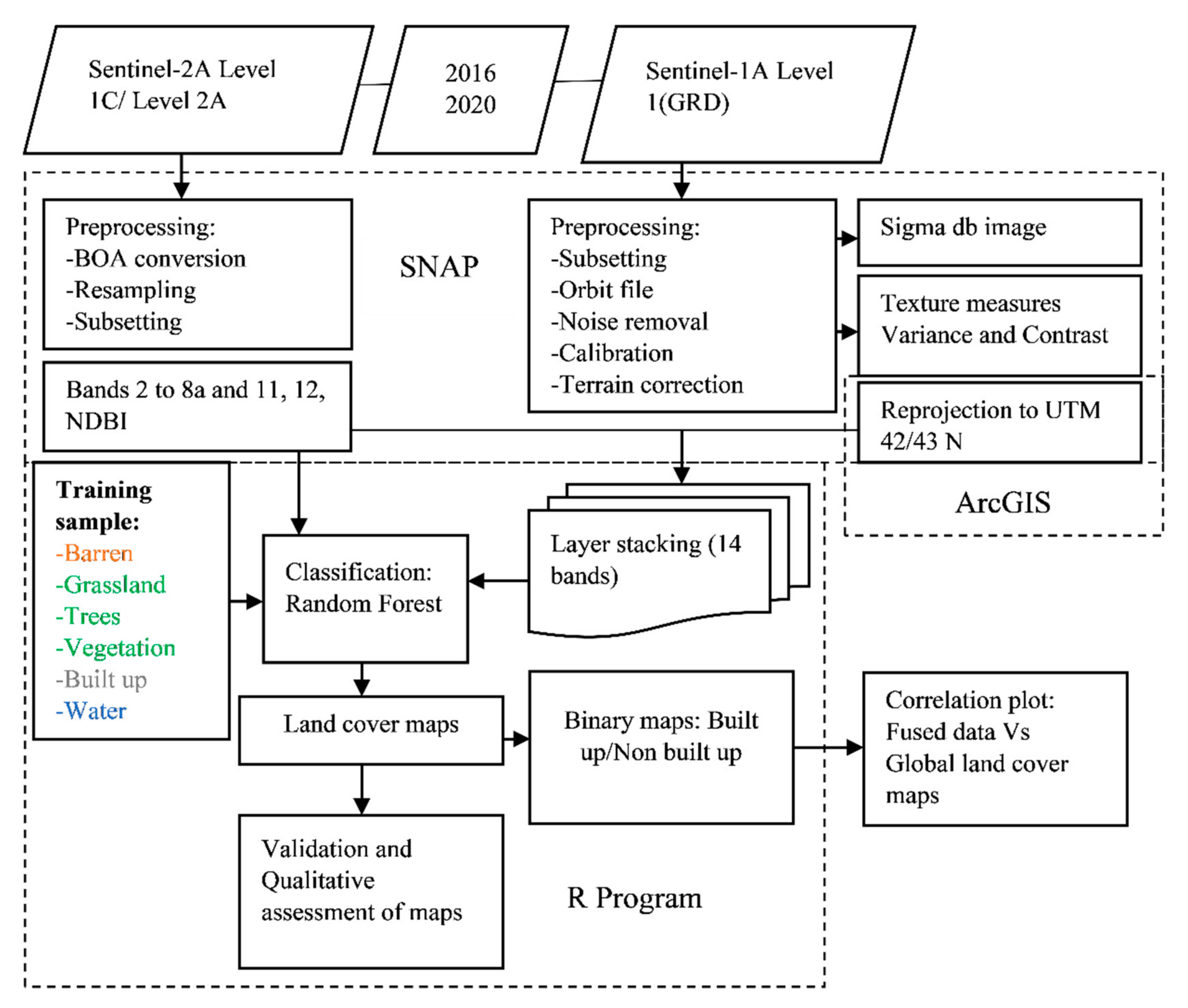
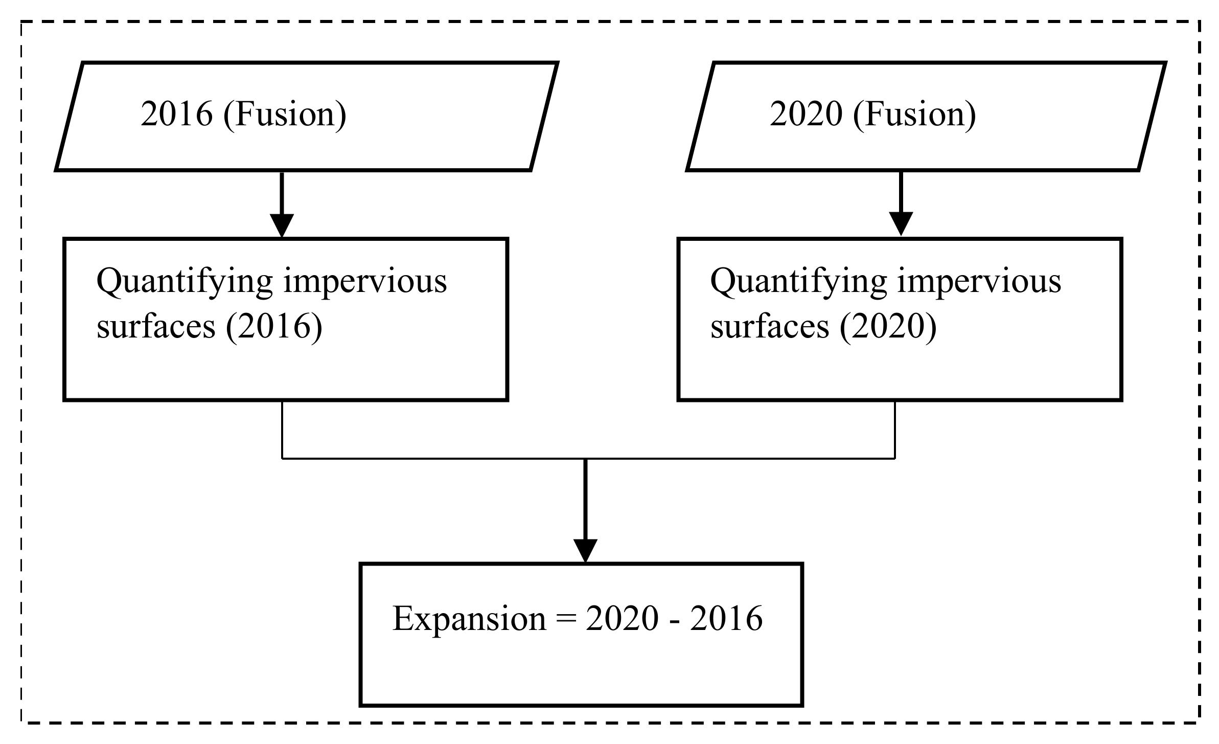
This section details the algorithms and processing used to combine the S-1 and S-2 images. It also covers the steps to map the impervious surfaces and quantify the growth rates of the nine Punjab cities for 2016 and 2020. There are five subsections of the method: image preprocessing, land cover classification, map validation, impervious surfaces quantification, and correlation analysis. Figure 2 shows a detailed flowchart of the research methodology and Figure 3 shows the steps for IS area quantification.
2.3.1. Image Preprocessing
The following section describes the preprocessing steps for radar and optical data, respectively. This study utilized the Sentinel Application Platform (SNAP) and ArcGIS pro for the process. Firstly, the coordinates given in Table 2 were used to subset the S-1 images for each city. The orbit files were then updated for accurate information on the position and velocity of the satellite. Then a calibration algorithm was applied to convert the raw digital number of each pixel to radiometrically calibrated SAR backscatter values called sigma naught. This was followed by the application of a range Doppler terrain correction algorithm to correct the distortion in the image due to the side looking geometry of the satellites. Finally, a logarithmic transformation of sigma naught values converted them to sigma dB values for end band composition. S-1 images are characterized by grainy structure called speckles which can be removed by speckle filtering in SNAP. However, [60] does not recommend the filtering when the interest is in the identification of small spatial structures, such as isolated houses or image textures, as the process may blur out important information.
For additional information from the radar images, grey level co-occurrence matrices (GLCM) were used to compute texture measures. According to [61,62], such measures capture the spatial relationships of pixels by identifying the pattern based on the neighborhood size provided. The resultant matrices store the occurrence frequency of pixel pairs with specific grey level (G) or pixel brightness values [61]. Such measures are common in image classification [63]. However, the texture measures must not be auto-correlated with each other according to [64]. Therefore, only contrast and variance were chosen, similar to [65]. For a neighborhood, a 5 × 5 moving widow was chosen, and single pixel displacement was used [65,66]. For a consistent classification result, VH polarization was eliminated from the 2020 images during the image sub-setting process. Then there were two additional bands in the form of texture measures in each radar image. Finally, all the SAR images were reprojected to UTM zone 42/43 to align with the extent and coordinate reference system (CRS) of their MSI pairs, using the bilinear interpolation resampling method in ArcGIS.
To convert the level 1C TOA products from 2016, sen2cor algorithms were applied in SNAP. They use the reflective properties of scene and cloud screening to create accurate atmospheric and surface parameters in the level 1 images. The corrections included cirrus correction, scene classification, aerosol optical thickness retrieval, and water vapor retrieval. The corrected image disregards band B10, as it only stores information on cirrus clouds [67]. A bilinear interpolation-based technique was used to resample 20 m and 60 m resolution optical bands to 10 m spatial resolution. Particularly bands B5, B6, B7, B8a, B11, and B12 to align with bands B2, B3, B4 and B8, and radar image (Table 5). The same city coordinates from Table 2 were used for the optical image sub setting. Bands B1 and B9 were eliminated because of their coarse spatial resolutions (originally 60 m) and aerosol and cloud sensitivity (ESA, 2015). There were ten bands in the final product (B2, B3, B4, B5, B6, B7, B8, B8a, B11, and B12.
Apart from same spatial resolution, the radar and optical images must be in same coordinate system and geometric extent to stack them into a single product. Therefore, while reprojecting radar image, a bilinear resampling method was used to align the radar image geometrically with optical image.
2.3.2. Land Cover Classification
After obtaining the processed images, the 10 optical bands, one band index, and texture and backscattering bands from radar data were stacked, and land cover maps were classified in R. A band index was developed using Equation (1) to highlight the built-up surfaces called normalized built-up index (NDBI).
Built-up surfaces have higher reflectance in band B11 according to [68]. Each image was loaded in R as a raster file, with bands as individual layers. Then using the “stack” command in R, ten bands and an index from the optical image were put together with a VV-polarization band and two texture measures from the radar image. This resulted in 14 bands, or layers, in a final raster stack image. Except for reflectance bands, sigma db, texture bands and band index were normalized before feeding them to the RF classifier. The resolution was preserved to 10 m in the final product. Such layer stacking is a form of pixel-based fusion technique for multisensory images. The following 14 layers were contained in the stacked image: Sentinel-1A VV amplitude image (1); Sentinel-1A VV variance texture image (1); Sentinel-1A VV contrast texture image (1); Sentinel-2A BOA reflectance bands 2 to 8a and 11 to 12 (10); and Sentinel-2A NDBI image (1).
Four land covers, vegetation, barren, water, and built up classifications were defined for each city; these were the dominant types of land cover in the cities. Built up cover included parking lots, road networks, buildings, and pavements, while vegetation included all tree cover, agricultural fields, fallow lands, and grasslands. Optical images alone, as well as stacked images, were then used to classify each city using the RF algorithm in R v.4.0.2.
RF uses bagging to create an ensemble of classification and regression tree (CART). It uses a random subset of variables each time to split at tree nodes to keep their inter-correlation minimal. They output the mode of class identified by each classifier tree [69,70]. Like a supervised classification approach, the RF model is trained with the land covers of interest across the remote sensing image scene [71,72,73].
Four RF models were prepared. The task included feeding land cover samples to train and test the model, defining RF parameters, and classifying the whole image. RF algorithms were developed by [74] and were implemented on the number of trees (ntree) and number of features in each split (mtry). The features are the 11 optical image bands and 14 stacked image bands. Generally, the square root of the total features present is used as the value of mtry, i.e., 4 in our case. A study conducted by [75] concluded that 500 is the optimum number of trees required for an RF classifier; thus 500 trees were used in this study. The land cover was assigned to each pixel based on the nearness of band values in the training set. Then each of 500 trees decide a particular cover for the pixel, and the most voted cover is the result.
2.3.3. Correlation Analysis
The resultant land cover maps were then reclassified into built-up and non-built-up surfaces, including vegetation, barren, and water cover, to emphasize the impervious surfaces of the cities. Then the resultant IS areas of each city from the fused data were correlated with the area of built-up surface in the global land cover maps for 2016 to assess their closeness. A graph was then plotted to compute the R squared value between the areas.
2.3.4. Test of Statistical Significance of Two Models
Two RF models were trained for each study year for each city. McNemar test was used to test statistical significance in extraction of built-up class for impervious surface mapping of the cities. It is applied to 2 × 2 contingency table with matched pairs of subject, correctly and incorrect classified built-up pixels by fused and optical data in this study. Then Chi-square values were computed for each city according to [76] as given in Equation (2). It compares the sensitivity and specificity of two datasets on land cover classification by finding out where the built-up pixels in classified maps disagree with each other [77].
where nf,o are number of samples correctly classified by RF model trained with fused data but incorrectly classified by RF model trained with optical alone data. Then the Chi-square value was checked for a threshold of 3.84 [76,77,78,79,80].
2.3.5. Impervious Surface Area and Expansion Rate Computation
Then pixel level area computation was performed to quantify the IS areas in each city using the fused data. The number of pixels identified as built-up class in the maps were multiplied by the spatial resolution of the images, i.e., 10 m, and converted into square km. Finally, the rate of urban expansion was computed for the past four years using Equation (3). The binary maps from 2015 were then overlaid on the maps from 2020 for further spatial analysis. Equation (3) is given by
where, R is the annual growth rate, n is the temporal gap, and I(2016) and I(2020) are the impervious surface area in 2015 and 2020 respectively for each city.
3. Results
In this section results from the current study are explained. The processed S-2 and combined S-1 and S-2 data were used to prepare land cover maps of each city with four classes: barren, vegetation, built-up, and water. Therefore, this section begins with RF models’ statistics and validation results of land cover maps followed by spectrum plot analysis. After establishing a premise for fused data results, the cities’ IS areas and expansion rates are presented. Finally, a correlation plot between the results from current study and Global Land Cover Maps are discussed.
3.1. RF Model Statistics and Land Cover Map Validation
Each of the four RF models trained for each city showed more than 95% overall accuracy (OA) and a kappa coefficient rate with the test datasets. This result is produced by the RF model based on test set prediction after adapting to the training sets. A confusion matrix was produced each time to compute the OA and kappa coefficients. The results support the claim that RF classifiers are known for their classification accuracy in the RS community [81].
After the RF models predicted each city’s whole image, the resultant land cover map was assessed with unique validation polygons. Validation samples were acquired for each land cover class. Automatic extraction or classification techniques need to be evaluated to develop confidence in the maps. Table 7 presents the accuracy assessment results for both optical and fused data. The accuracy evaluations were performed by computing the OA and kappa coefficients from the CM. OA is the ratio of the sum of diagonal elements and total elements in the CM. The kappa coefficient is the ratio of correctly predicted elements and total elements, considering the misclassified elements as well, from the CM. According to [82] a kappa coefficient gives a more robust accuracy assessment, as it considers both predicted classification and referenced classification data. A kappa value ranging from 0.8 to 1 is considered a highly accurate match with the reference values [83].
3.2. Correlation Analysis
Table 8
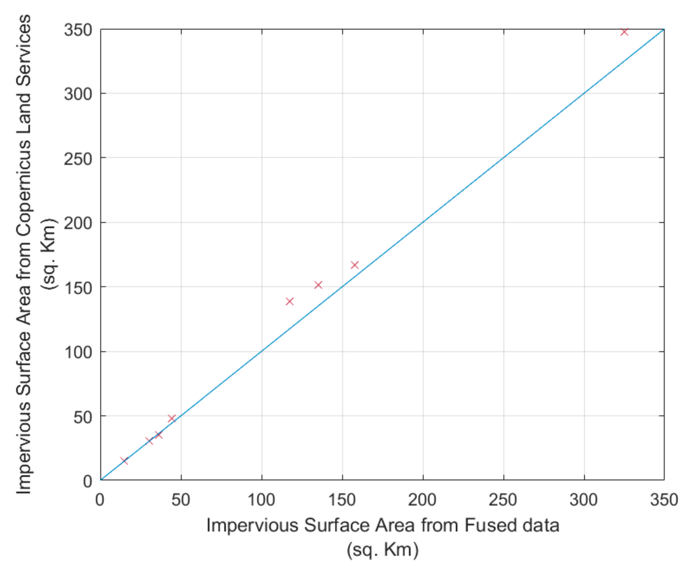
lists the IS areas of the cities in 2016 from fused and global datasets. For further assessment of land cover maps, quantitative validation with CLS was performed. In Figure 4, the IS area from CLS is given on the y-axis, and the result from the current study is plotted on the x-axis. The minimum impervious area estimated was 14.8 km2 in the smallest city Khanewal and the maximum estimated impervious area was 324.9 km2 in the largest city Rawalpindi–Islamabad. The correlation of the estimated impervious area by the RF models and the CLS data showed a strong linear relationship with an R-squared value of 0.99. The RMSD calculated between the estimation and the CLS data was 12.8 km2 which is 11.8% of the average of the estimated areas. From the plots, an underestimation of the IS was seen compared to the global data, as the slope of the point data was 1.0789, with an intercept of 0.36 km2. The average underestimation was 9.05 km2. The Pearson correlation test was conducted with a 95% confidence limit. Thus, based on the accuracies of the classified maps, strong linearity to independent datasets, and an analysis from the spectrum plots, IS area was quantified and urban expansion rates were computed from fused datasets only.
3.3. Test of Statistical Significance
Although, from Table 7, the improvement in OA and kappa coefficients were not significant in many cities, McNemar test results highlight that the classification of built-up pixels by two different RF models: trained with fused data and trained with optical data are statistically significant. The Chi square value obtained from the 2 × 2 confusion matrices of Rawalpindi–Islamabad, Multan, Faisalabad, Gujranwala, Bahawalpur, Sahiwal, Sheikhupura and Khanewal are given in Table 9. The Chi-square values are larger than or equal to 3.84 and p-values are less than 0.05 for all cities at 95% confidence limit. The result confirms the better performance of fused dataset over optical alone.
3.4. Impervious Surface Area and Cities’ Expansion Rates
Table 10 shows the IS areas of all nine cities from the fused data of 2016 and 2020 and corresponding cumulative growth of the cities in the past four years. From the Table, it is seen that the urbanized surface of Rawalpindi–Islamabad grew from 324.9 km2 in 2016 to 358.1 km2 in 2020. The total growth of the city is 10.2%, with an annual rate of 2.5%. It has the highest growth in terms of km2 and the 2nd highest growth rate in terms of percentage among the cities considered. RI is also the largest in the list in terms of area as well as population. Since Rawalpindi and Islamabad share the same border, they are jointly known as a twin city. They have a combined population of more than 3 million as of the 2017 census. The smallest city in the list, Khanewal, had urbanized surface growth from 14.6 km2 to 14.9 km2 with the lowest expansion rate. Additionally, the cumulative growth of Multan was 6.3%, Faisalabad was 9.7% Gujranwala was 8.1%, Bahawalpur was 11.8%, Sahiwal was 8.3%, and Sheikhupura was 9.3%. Overall, IS expansion was seen in all nine cities studied.
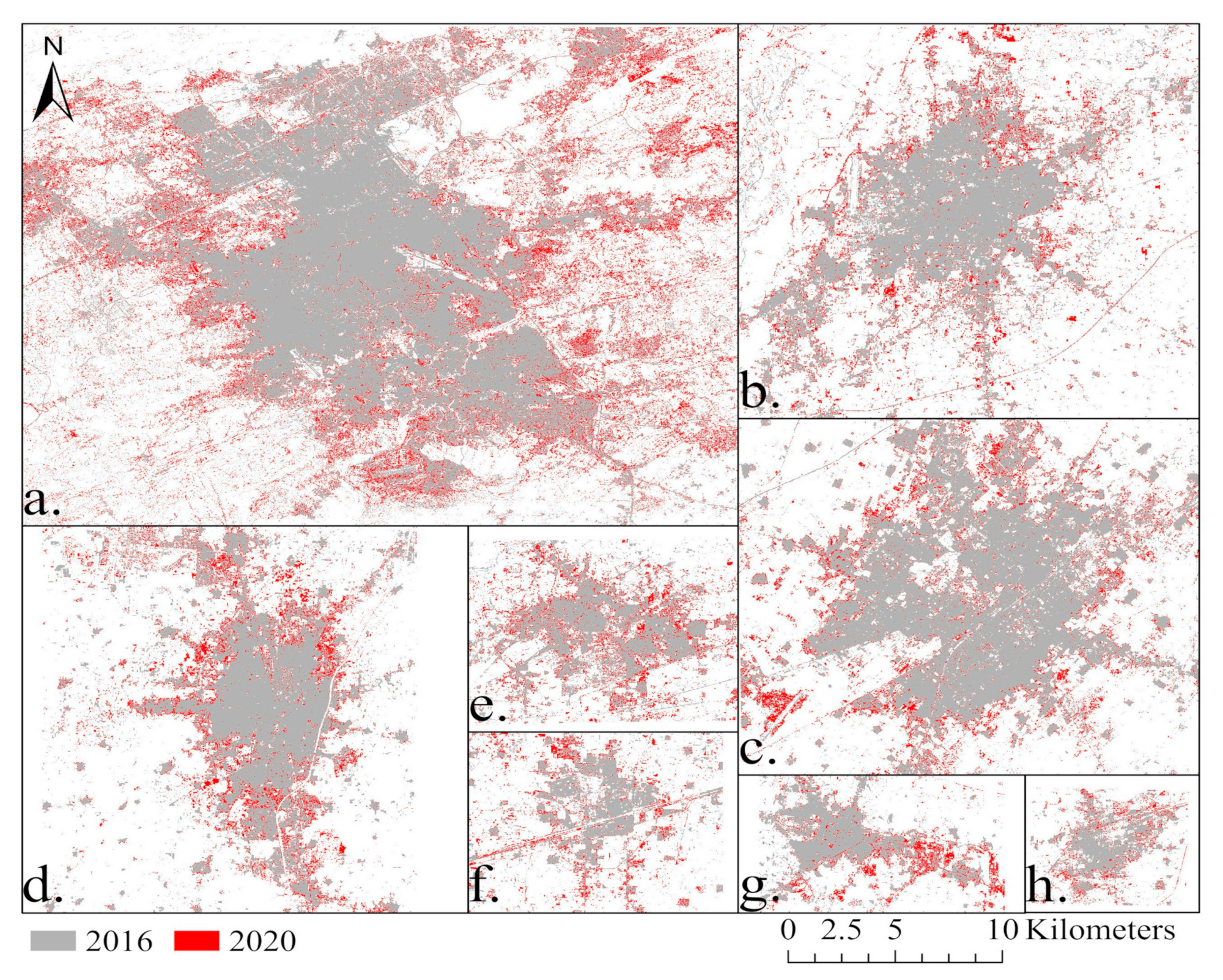
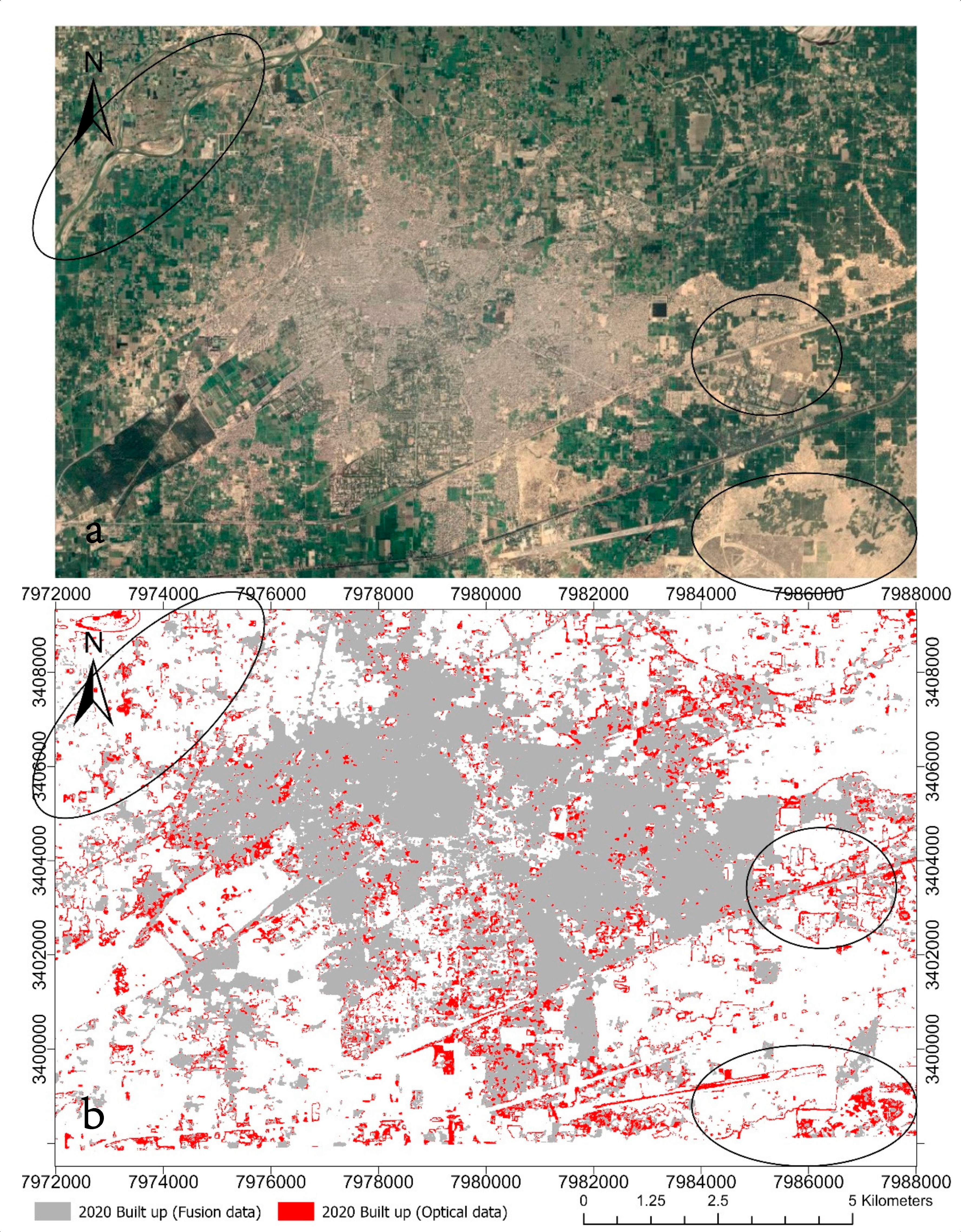
Figure 5 shows the IS expansion from 2016 to 2020 in the studied cities. The 2016 binary maps were overlaid on top of 2020 maps to identify growth patterns in these cities. The area in red is the IS added in the cities in the last four years. As seen in the figure, expansion took place mostly on the cities’ outskirts. There are some infill growths as well. Increases in IS within the areas surrounded by urban surfaces in 2016 are seen in all cities. The north of Multan (Figure 5b), east of Sheikhupura (Figure 5g), and northwest of Sahiwal (Figure 5f) also had significant growth. Since the temporal gap between the analyses of urban expansion was just four years in our study, a thorough review of the growth pattern is challenging. In summary the most predominant type of urban growths were infill growth and edge expansion. In the former development of new built-up surface is surrounded by preexisting built up surface [84]. And in the latter newly developed built-up surface spreads out from the edge of an existing built-up surface [84] also known as edge development [85]. Infill is common to places with preexisting urban services such as water, road, and sewers according to [84].
4. Discussion
It is apparent from the results in Table 7 that in all cities either in one or both time periods, the OA and kappa coefficients of the classified maps from fused datasets show improvement. There is a 2 to 9% increase in OA and a 3 to 12 % increase in kappa coefficient. Such instances emphasize the potentiality of S-1 data to add values to the cities’ impervious surfaces mapping relative to S-2 data alone.
The low resolution (100 m) Proba-V images used by the global dataset tended to overestimate the IS in most of the cities (refer Table 8), as the pixels were likely to mix the coexisting heterogeneous covers. In [26,27,86,87,88] the authors also argue on the inadequacy of coarse spatial resolution in representing spatial disparity within cities. From the HRI, many city locations were identified with a mixture of tree cover, grassland, water canal, buildings, and other open spaces. Different land covers in such proximity require high resolution images for clear discrimination. Thus, in comparison to global datasets, the results from fused data underestimated the values ranging from 0.5% to 15%.
Authors from [89] used the McNemar test in their study to test the statistical significance in the difference of classification result from maximum likelihood classification (MLC) and Iterative Self-Organizing Data Analysis Technique and texture analysis (Iso-Tex) classification. Similar to this study, [89] also emphasizes on extraction of built-up cover to map impervious surfaces. They have utilized SAR images and derived texture bands (energy, mean and variance) from Sentinel-1. According to [90], heterogenous urban areas have distinct spectral signature on SAR images. [89] concluded the potentiality of texture information in discriminating built-up areas from other land covers such as green areas, bare soil, and water bodies in urban areas. They found the most significant difference on variance texture band for VV based on the highest mean percentage difference on spectral signature between urban and non-urban areas. Significant contribution of variance texture band was also identified in this study through the spectrum plots.
From the spectral signature plots, valuable information added by the radar bands in the land cover classification is identified. In the sigma dB backscattering band and the variance texture derived from radar image, built up cover had the highest value, which could be important information for the RF classifiers. Such a distinct feature is helpful for the classifier in differentiating different land covers. This might have improved the overall accuracy and kappa coefficient of classified maps from the fused dataset. One of the constraints of optical images is limited spectral resolution, which causes different building roofs, roads, and parking lots to appear as different colors. Similarly, high spectral variation within the same land cover type and low spectral variation between different land cover types may occur in urban areas. Therefore, sole reliance on optical bands for land cover classification is not recommended. This makes the automatic extraction of impervious surfaces challenging [91]. Therefore, [92,93,94,95,96] suggest texture as one of the measures to reduce the impact of spectral variation within the same land cover (as cited in [70]). With free access S-1 datasets, calculation of texture measures is possible with low computational cost, unlike in the past.
Figure 6 shows land cover maps of Rawalpindi–Islamabad from optical and fused data, respectively. They are the northernmost cities considered in this study. Unlike all other cities with flat topography, a part of the Siwalik Range surrounds Rawalpindi and neighboring Islamabad to the north. The encircled region in Figure 6a depicts that the map from optical data misclassified vegetation into water. According to [97,98], topographic shadows of irregular mountains create a major obstacle in accurate land cover classification while using optical images. Such shadows are often misclassified as water as both have very low reflectance [99]. Therefore, shadow removal techniques were applied during classification [97,98]. Shadows commonly occur in high resolution optical images in the form of dark features, reducing the spectral values of shaded objects affecting the land cover classification. One of the sources of shadow in urban areas are tall buildings [100]. Thus, built up surfaces in such areas are likely to be misclassified as water. In their study [100] performs a hierarchical classification method to first extract shadow and non-shadow areas and divide the latter into parking lots and non-parking lots to finally classify buildings and roads. They use band indices such as brightness, normalized difference water index (NDWI), and Ration G, through thresholding and vector data, to discriminate shadows. A study in [97] used DEM data and various topographic correction methods, such as improved cosine correction, C-correction, Minnaert correction, statistical empirical corrections, and a variable empirical coefficient algorithm to reduce relief effects in forest cover classification of a complex mountainous topography. In contrast Figure 6b shows that misclassified water pixels were significantly reduced by the fused dataset. This demonstrates the usefulness of radar bands to eliminate shadow effects without any correction algorithm. Unlike the optical image, radar images consider the geometry of the object backscattering the signal. Also surface roughness and internal structure of the surface can be retrieved. Therefore, inclusion of derived texture measures from the radar band can reduce the shadow effects without any complex topographic correction or complex shadow removal techniques.
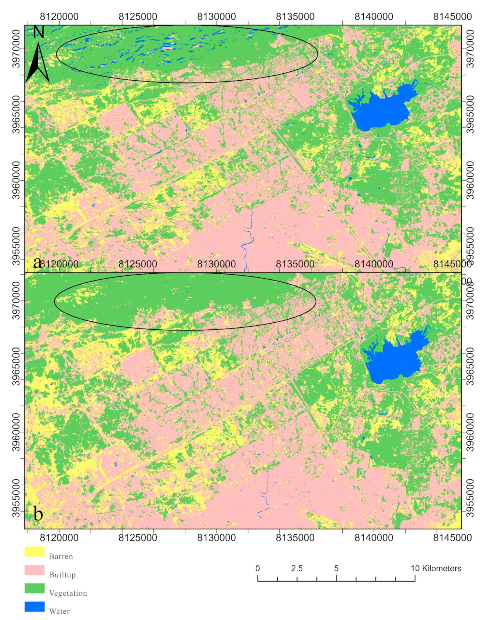
Most of the cities considered in this study are surrounded by cultivation and other vegetation cover. In contrast, Bahawalpur has significant barren cover to its south and east that can also be seen in Figure 7a. The 2020 optical data overestimated Bahawalpur’s impervious surface area by over 20%. Therefore, the city’s impervious surface map from fused data was overlaid on the impervious surface map from optical data for further examination. In Figure 7b it is seen that considerable barren pixels were misclassified as built-up to the south and east, as well as on the riverbanks. Misclassification of barren surface into built up was also observed in other cities lying on the riverbank (Multan and Rawalpindi). The impervious surfaces overestimation from optical data alone in other cities ranged from 1.5% in Sahiwal to 7.1% in Multan, for 2020. A similar case was also observed in a study conducted by [101] where river sand class was misclassified into built-up class. The built-up area extraction from spectral or spatial indexes or spectral alone data does not address the confusion between built-up and other land cover types as it emphasizes a single class [102]. Due to heterogeneous spectral characteristics of urban areas, spectral confusion is created with other land cover classes. For instance, similar spectral signatures of barren land and asphalt concrete results in misclassification of barren into built-up and vice versa during land cover classification. Therefore, texture measures are widely used in built-up area extraction [103,104,105,106,107,108]. Each texture measure obtained from the radar band provides unique spatial information to discriminate between land cover types [102] and can complement reflectance information from optical images.
IS expansion in these cities occurred at a cost of replacing natural surfaces, such as agricultural land, open spaces, and tree cover with built-up surfaces. Increasing such surfaces surges the wastewater and stormwater effluents. If such effluent is directed to streams without proper treatment, both humans and aquatic lives are at risk [109,110]. Authors in [111] performed water quality modeling of the Ravi River in their study. Drainage of various urban areas of Sheikhupura, Faisalabad, and Sahiwal districts ultimately carry the untreated effluent into the river [112,113]. They identified a distinct difference between the water quality upstream of the river and at downstream locations in vicinity to urban settlements. The latter resulted in high concentrations of total dissolved solids (TDS), ammonia, and other toxic compounds [111]. Like the Ravi, the Chenab River also faced adverse contamination with cadmium and lead, as identified by [114]. Their results revealed rapid urbanization as one of the major sources of metal pollution. Urban heat island (UHI) effects are another consequence [115,116]. For instance, [117] identified a 1.52 °C average warming effect in Islamabad from 1993 to 2018, due to the city’s increased IS. Thus, knowledge of IS spatial distribution in cities can aid in addressing the urban climate and environmental pollution issues.
5. Methodology Transfer and Limitation
Fusion of S-1 and S-2 data as a single, stacked product requires both images to have same spatial resolution, coordinate reference system, and geometric alignment. However, to replicate the process in tropical regions would be challenging for impervious surfaces mapping, with S-2 being data constantly contaminated with cloud covers [45,64]. The temporal gap between images must not be large to avoid biases in the classification. Besides, availability of Sentinel data, starting in 2014–2015, prevents the user from long term assessment of impervious surfaces expansion. For a larger study area, the method can be computationally time consuming. The technique would mainly benefit urban areas with open spaces within the settlement due to higher spatial resolution of Sentinel data [26,27,84,85,86] despite the urban density.
6. Conclusions
In this study S-1 combined with S-2 were used to quantify the IS of nine Pakistani cities (Rawalpindi–Islamabad, Multan, Faisalabad, Gujranwala, Bahawalpur, Sahiwal, Sheikhupura, and Khanewal) in 2016 and 2020. It also estimated the rates of expansion in those cities. An RF classifier was used for land cover classification defined by four classes: barren, built-up, vegetation, and water. The maps were reclassified into binary maps to emphasize the IS. The results from optical and combined data were analyzed and values added by S-1 were interpreted with the support of land cover maps.
Results show that the IS expansion took place in all cities under consideration. Rawalpindi–Islamabad had the highest growth among the cities considered, with the rate of 2.5%, while Khanewal had the least growth, with a rate of 0.5%. The annual expansion rates of the remaining cities ranged from 1% to 2.25%. From CM there was a 2% to 9% increase in OA and a 3% to 12 % increase in kappa coefficient of the classified maps. Spectrum plots showed built up surfaces had the highest values in backscattering and variance texture bands. This could have contributed to improving map accuracies. Besides, in several optical bands, the signatures of barren soil were in the vicinity of the built-up surface. This likely resulted in the overestimation of IS from optical data. The maximum overestimation was seen in the city with significant barren cover on the periphery, i.e., Bahawalpur. The overestimation was more than 20%. However, S-1 was able to remove the misclassified topography shadows into water in the land cover maps of Rawalpindi. Such phenomena are common in places with irregular topography, according to past studies. Estimation of IS in cities surrounded with irregular topography and significant barren surfaces can be improved by using fused radar and optical dataset. Thus, this study was able to develop a cost and labor effective methodology to combine radar and optical data to improve impervious surface mapping at a city scale. This will aid in updating information on impervious surfaces, as well as present and future trends of a city’s expansion.
Author Contributions
All three authors contributed equally to conceptualization of the research. B.S. prepared the methodology which included curating data, training the classifier and validating the classified maps. Substantial technical help was provided by H.S. for software operation while both H.S. and S.A. contributed equally to formal analysis and investigation of the result. Original draft was prepared by B.S. while the writing was reviewed and edited by H.S. and S.A. Manuscript was finalized under the supervision of S.A. and H.S. All authors have read and agreed to the published version of the manuscript.
Funding
This research received no external funding.
Data Availability Statement
The data that support the finding of this study are available from the corresponding author upon the reasonable request. Due to privacy concern the link to the drive where the data are deposited is not provided publicly.
Acknowledgments
The publication fees for this article were supported by the UNLV University Libraries Open Article Fund. The authors would like to acknowledge the technological support provided by the Office of Information Technology (OIT) at University of Nevada, Las Vegas.
Conflicts of Interest
The authors declare no conflict of interest.
References
- United Nations. United Nations Expert Group Meeting on Population Distribution, Urbanization, Internal Migration and Development. United Nations Population Division. 2008. Available online: https://sustainabledevelopment.un.org/content/documents/2529P01_UNPopDiv.pdf (accessed on 1 February 2021).
- Angel, S.; Blei, A.M.; Civco, D.L.; Parent, J. Atlas of Urban Expansion; Lincoln Institute of Land Policy: Cambridge, MA, USA, 2012; p. 397. [Google Scholar]
- Berry, B.J. Urbanization. In Urban Ecology; Springer: Boston, MA, USA, 2008; pp. 25–48. [Google Scholar]
- Imbe, M.; Ohta, T.; Takano, N. Quantitative assessment of improvements in hydrological water cycle in urbanized river basins. Water Sci. Technol. 1997, 36, 219–222. [Google Scholar] [CrossRef]
- Nascimento, N.O.; Ellis, J.B.; Baptista, M.B.; Deutsch, J.C. Using detention basins: Operational experience and lessons. Urban Water 1999, 1, 113–124. [Google Scholar] [CrossRef]
- Wickham, J.D.; O’Neill, R.V.; Riitters, K.H.; Smith, E.R.; Wade, T.G.; Jones, K.B. Geographic targeting of increases in nutrient export due to future urbanization. Ecol. Appl. 2002, 12, 93–106. [Google Scholar] [CrossRef]
- Jones, J.A.; Swanson, F.J.; Wemple, B.C.; Snyder, K.U. Effects of roads on hydrology, geomorphology, and disturbance patches in stream networks. Conserv. Biol. 2000, 14, 76–85. [Google Scholar] [CrossRef]
- Gao, F.; De Colstoun, E.B.; Ma, R.; Weng, Q.; Masek, J.G.; Chen, J.; Pan, Y.; Song, C. Mapping impervious surface expansion using medium-resolution satellite image time series: A case study in the Yangtze River Delta, China. Int. J. Remote Sens. 2012, 33, 7609–7628. [Google Scholar] [CrossRef]
- Arnold, C.L., Jr.; Gibbons, C.J. Impervious surface coverage: The emergence of a key environmental indicator. J. Am. Plan. Assoc. 1996, 62, 243–258. [Google Scholar] [CrossRef]
- Thakali, R.; Kalra, A.; Ahmad, S. Understanding the Effects of Climate Change on Urban Stormwater Infrastructures in the Las Vegas Valley. Hydrology 2016, 3, 34. [Google Scholar] [CrossRef] [Green Version]
- Thakali, R.; Kalra, A.; Ahmad, S.; Qaiser, K. Management of an Urban Stormwater System Using Projected Future Scenarios of Climate Models: A Watershed-Based Modeling Approach. Open Water J. 2018, 5, 1–17. [Google Scholar]
- Forsee, W.; Ahmad, S. Evaluating Urban Stormwater Infrastructure Design in Response to Projected Climate Change. ASCE J. Hydrol. Eng. 2011, 16, 865–873. [Google Scholar] [CrossRef]
- Rahaman, M.M.; Thakur, B.; Kalra, A.; Ahmad, S. Modeling of GRACE-Derived Groundwater Information in the Colorado River Basin. Hydrology 2019, 6, 19. [Google Scholar] [CrossRef] [Green Version]
- Mistry, G.; Stephen, H.; Ahmad, S. Impact of Precipitation and Agricultural Productivity on Groundwater Storage in Rahim Yar Khan District, Pakistan. In Proceedings of the World Environmental and Water Resources Congress, Pittsburg, PA, USA, 19–23 May 2019; pp. 104–117. [Google Scholar]
- Bukhary, S.; Batista, J.; Ahmad, S. Analyzing Land and Water Requirements for Solar Deployment in the Southwestern United States. Renew. Sustain. Energy Rev. 2018, 82, 3288–3305. [Google Scholar] [CrossRef]
- Chen, C.; Kalra, A.; Ahmad, S. A Conceptualized Groundwater Flow Model Development for Integration with Surface Hydrology Model. In Proceedings of the World Environmental and Water Resources Congress, Sacramento, CA, USA, 21–25 May 2017; pp. 175–187. [Google Scholar] [CrossRef] [Green Version]
- Klein, R. Urbanization and stream quality impairment. Am. Water Resour. Assoc. Water Resour. Bull. 1979, 15, 948–963. [Google Scholar] [CrossRef]
- Harbor, J.M. A practical method for estimating the impact of land-use change on surface runoff, groundwater recharge and wetland hydrology. J. Am. Plan. Assoc. 1994, 60, 95–108. [Google Scholar] [CrossRef]
- Pappas, E.A.; Smith, D.R.; Huang, C.; Shuster, W.D.; Bonta, J.V. Impervious surface impacts to runoff and sediment discharge under laboratory rainfall simulation. Catena 2008, 72, 146–152. [Google Scholar] [CrossRef]
- Schueler, T.R.; Fraley-McNeal, L.; Cappiella, K. Is impervious cover still important? Review of recent research. J. Hydrol. Eng. 2009, 14, 309–315. [Google Scholar] [CrossRef] [Green Version]
- Hurd, J.D.; Civco, D.L. Temporal characterization of impervious surfaces for the State of Connecticut. In Proceedings of the ASPRS Annual Conference, Denver, CO, USA, 23–28 May 2004. [Google Scholar]
- Bhatta, B. Analysis of Urban Growth and Sprawl from Remote Sensing Data; Springer Science & Business Media: Berlin, Germany, 2010. [Google Scholar]
- Zhou, Q.; Mikkelsen, P.S.; Halsnæs, K.; Arnbjerg-Nielsen, K. Framework for economic pluvial flood risk assessment considering climate change effects and adaptation benefits. J. Hydrol. 2012, 414, 539–549. [Google Scholar] [CrossRef]
- Slonecker, E.T.; Jennings, D.B.; Garofalo, D. Remote sensing of impervious surfaces: A review. Remote Sens. Rev. 2001, 20, 227–255. [Google Scholar] [CrossRef]
- Townshend, J.; Justice, C.; Li, W.; Gurney, C.; McManus, J. Global land cover classification by remote sensing: Present capabilities and future possibilities. Remote Sens. Environ. 1991, 35, 243–255. [Google Scholar] [CrossRef]
- Loveland, T.R.; Reed, B.C.; Brown, J.F.; Ohlen, D.O.; Zhu, Z.; Yang, L.W.M.J.; Merchant, J.W. Development of a global land cover characteristics database and IGBP DISCover from 1 km AVHRR data. Int. J. Remote Sens. 2000, 21, 1303–1330. [Google Scholar] [CrossRef]
- Friedl, M.A.; McIver, D.K.; Hodges, J.C.; Zhang, X.Y.; Muchoney, D.; Strahler, A.H.; Woodcock, C.; Gopal, S.; Schneider, A.; Cooper, A.; et al. Global land cover mapping from MODIS: Algorithms and early results. Remote Sens. Environ. 2002, 83, 287–302. [Google Scholar] [CrossRef]
- Mayaux, P.; Bartholomé, E.; Fritz, S.; Belward, A. A new land-cover map of Africa for the year 2000. J. Biogeogr. 2004, 31, 861–877. [Google Scholar] [CrossRef]
- Bicheron, P.; Defourny, P.; Brockmann, C.; Schouten, L.; Vancutsem, C.; Huc, M.; Bontemps, S.; Leroy, M.; Achard, F.; Herold, M.; et al. Globcover: Products Description and Validation Report. 2008. Available online: https://www.researchgate.net/publication/260137807_GLOBCOVER_products_description_and_validation_report (accessed on 20 February 2021).
- Hansen, M.C.; Potapov, P.V.; Moore, R.; Hancher, M.; Turubanova, S.A.; Tyukavina, A.; Thau, D.; Stehman, S.V.; Goetz, S.J.; Loveland, T.R.; et al. High-resolution global maps of 21st-century forest cover change. Science 2013, 342, 850–853. [Google Scholar] [CrossRef] [PubMed] [Green Version]
- Poudel, U.; Stephen, H.; Ahmad, S. Evaluating Irrigation Performance and Water Productivity Using EEFlux ET and NDVI. Sustainability 2021, 13, 7967. [Google Scholar] [CrossRef]
- Joshi, N.; Baumann, M.; Ehammer, A.; Fensholt, R.; Grogan, K.; Hostert, P.; Jepsen, M.R.; Kuemmerie, T.; Meyfroidt, P.; Mitchard, E.T.A.; et al. A review of the application of optical and radar remote sensing data fusion to land use mapping and monitoring. Remote Sens. 2016, 8, 70. [Google Scholar] [CrossRef] [Green Version]
- Pohl, C.; Van Genderen, J.L. Review article multisensor image fusion in remote sensing: Concepts, methods and applications. Int. J. Remote Sens. 1998, 19, 823–854. [Google Scholar] [CrossRef] [Green Version]
- Stefanski, J.; Kuemmerle, T.; Chaskovskyy, O.; Griffiths, P.; Havryluk, V.; Knorn, J.; Korol, N.; Sieber, A.; Waske, B. Mapping land management regimes in western Ukraine using optical and SAR data. Remote Sens. 2014, 6, 5279–5305. [Google Scholar] [CrossRef] [Green Version]
- Brisco, B.; Brown, R.J. Multidate SAR/TM synergism for crop classification in western Canada. Photogramm. Eng. Remote Sens. 1995, 61, 1009–1014. [Google Scholar]
- Chust, G.; Ducrot, D.; Pretus, J.L. Land cover discrimination potential of radar multitemporal series and optical multispectral images in a Mediterranean cultural landscape. Int. J. Remote Sens. 2004, 25, 3513–3528. [Google Scholar] [CrossRef]
- Huang, H.; Legarsky, J.; Othman, M. Land-cover classification using Radarsat and Landsat imagery for St. Louis 2007, Missouri. Photogramm. Eng. Remote Sens. 2007, 73, 37–43. [Google Scholar] [CrossRef] [Green Version]
- Attema, E.; Davidson, M.; Floury, N.; Levrini, G.; Rosich, B.; Rommen, B.; Snoeij, P. Sentinel-1 ESA’s new European radar observatory. In Proceedings of the 7th European Conference on Synthetic Aperture Radar, Friedrichshafen, Germany, 2–5 June 2008; pp. 1–4. [Google Scholar]
- Richards, J.A.; Jia, X. The interpretation of digital image data. In Remote Sensing Digital Image Analysis; Springer: Heidelberg/Berlin, Germany, 1999; pp. 75–88. [Google Scholar]
- Gislason, P.O.; Benediktsson, J.A.; Sveinsson, J.R. Random forests for land cover classification. Pattern Recognit. Lett. 2006, 27, 294–300. [Google Scholar] [CrossRef]
- Steinhausen, M.J.; Wagner, P.D.; Narasimhan, B.; Waske, B. Combining Sentinel-1 and Sentinel-2 data for improved land use and land cover mapping of monsoon regions. Int. J. Appl. Earth Obs. Geoinf. 2018, 73, 595–604. [Google Scholar] [CrossRef]
- Denize, J.; Hubert-Moy, L.; Betbeder, J.; Corgne, S.; Baudry, J.; Pottier, E. Evaluation of using sentinel-1 and-2 time-series to identify winter land use in agricultural landscapes. Remote Sens. 2019, 11, 37. [Google Scholar] [CrossRef] [Green Version]
- Van Tricht, K.; Gobin, A.; Gilliams, S.; Piccard, I. Synergistic use of radar Sentinel-1 and optical Sentinel-2 imagery for crop mapping: A case study for Belgium. Remote Sens. 2018, 10, 1642. [Google Scholar] [CrossRef] [Green Version]
- Hedayati, P.; Bargiel, D. Fusion of Sentinel-1 and Sentinel-2 images for classification of agricultural areas using a novel classification approach. In Proceedings of the IGARSS 2018–2018 IEEE International Geoscience and Remote Sensing Symposium, Valencia, Spain, 22–27 July 2018; pp. 6643–6646. [Google Scholar]
- Lu, L.; Tao, Y.; Di, L. Object-based plastic-mulched landcover extraction using integrated Sentinel-1 and Sentinel-2 data. Remote Sens. 2018, 10, 1820. [Google Scholar] [CrossRef] [Green Version]
- Erinjery, J.J.; Singh, M.; Kent, R. Mapping and assessment of vegetation types in the tropical rainforests of the Western Ghats using multispectral Sentinel-2 and SAR Sentinel-1 satellite imagery. Remote Sens. Environ. 2018, 216, 345–354. [Google Scholar] [CrossRef]
- Whyte, A.; Ferentinos, K.P.; Petropoulos, G.P. A new synergistic approach for monitoring wetlands using Sentinels-1 and 2 data with object-based machine learning algorithms. Environ. Model. Softw. 2018, 104, 40–54. [Google Scholar] [CrossRef] [Green Version]
- Iannelli, G.C.; Gamba, P. Jointly exploiting Sentinel-1 and Sentinel-2 for urban mapping. In Proceedings of the IGARSS 2018–2018 IEEE International Geoscience and Remote Sensing Symposium, Valencia, Spain, 22–27 July 2018; pp. 8209–8212. [Google Scholar]
- Gao, Q.; Zribi, M.; Escorihuela, M.J.; Baghdadi, N. Synergetic use of Sentinel-1 and Sentinel-2 data for soil moisture mapping at 100 m resolution. Sensors 2017, 17, 1966. [Google Scholar]
- Tavus, B.; Kocaman, S.; Nefeslioglu, H.A.; Gokceoglu, C. A fusion approach for flood mapping using Sentinel-1 and Sentinel-2 datasets. Int. Arch. Photogramm. Remote Sens. Spat. Inf. Sci. 2020, 43, 641–648. [Google Scholar] [CrossRef]
- Manakos, I.; Kordelas, G.A.; Marini, K. Fusion of Sentinel-1 data with Sentinel-2 products to overcome non-favourable atmospheric conditions for the delineation of inundation maps. Eur. J. Remote Sens. 2020, 53 (Suppl. S2), 53–66. [Google Scholar]
- Kpienbaareh, D.; Sun, X.; Wang, J.; Luginaah, I.; Bezner Kerr, R.; Lupafya, E.; Dakishoni, L. Crop type and land cover mapping in northern Malawi using the integration of sentinel-1, sentinel-2, and planetscope satellite data. Remote Sens. 2021, 13, 700. [Google Scholar] [CrossRef]
- Heckel, K.; Urban, M.; Schratz, P.; Mahecha, M.D.; Schmullius, C. Predicting forest cover in distinct ecosystems: The potential of multi-source Sentinel-1 and-2 data fusion. Remote Sens. 2020, 12, 302. [Google Scholar] [CrossRef] [Green Version]
- Hong, D.; Gao, L.; Yokoya, N.; Yao, J.; Chanussot, J.; Du, Q.; Zhang, B. More diverse means better: Multimodal deep learning meets remote-sensing imagery classification. IEEE Trans. Geosci. Remote Sens. 2020, 59, 4340–4354. [Google Scholar]
- Tavares, P.A.; Beltrão, N.E.S.; Guimarães, U.S.; Teodoro, A.C. Integration of sentinel-1 and sentinel-2 for classification and LULC mapping in the urban area of Belém, eastern Brazilian Amazon. Sensors 2019, 19, 1140. [Google Scholar] [CrossRef] [PubMed] [Green Version]
- Corbane, C.; Faure, J.F.; Baghdadi, N.; Villeneuve, N.; Petit, M. Rapid urban mapping using SAR/optical imagery synergy. Sensors 2008, 8, 7125–7143. [Google Scholar] [CrossRef] [PubMed]
- Gamba, P.; Dell’Acqua, F.; Dasarathy, B.V. Urban remote sensing using multiple data sets: Past, present, and future. Inf. Fusion 2005, 6, 319–326. [Google Scholar] [CrossRef]
- McNemar, Q. Note on the sampling error of the difference between correlated proportions or percentages. Psychometrika 1947, 12, 153–157. [Google Scholar] [CrossRef]
- Mukhtar, U.; Zhangbao, Z.; Beihai, T.; Naseer, M.A.U.R.; Razzaq, A.; Hina, T. Implications of decreasing farm size on urbanization: A case study of Punjab Pakistan. J. Soc. Sci. Stud. 2018, 5, 71–86. [Google Scholar] [CrossRef] [Green Version]
- Filipponi, F. Sentinel-1 GRD preprocessing workflow. In Proceedings of the 3rd International Electronic Conference on Remote Sensing, In the Internet Environment, 22 May–5 June 2019; Volume 18, p. 11. Available online: https://sciforum.net/conference/ecrs-3 (accessed on 1 June 2021).
- Haralick, R.M.; Shanmugam, K.; Dinstein, I.H. Textural features for image classification. IEEE Trans. Syst. Man Cybern. 1973, SMC-3, 610–621. [Google Scholar] [CrossRef] [Green Version]
- Jenicka, S.; Suruliandi, A. A textural approach for land cover classification of remotely sensed images. CSI Trans. ICT 2014, 2, 1–9. [Google Scholar] [CrossRef] [Green Version]
- Abdel-Hamid, A.; Dubovyk, O.; El-Magd, A.; Menz, G. Mapping mangroves extend on the Red Sea coastline in Egypt using polarimetric SAR and high resolution optical remote sensing data. Sustainability 2018, 10, 646. [Google Scholar] [CrossRef] [Green Version]
- Hall-Beyer, M. Practical guidelines for choosing GLCM textures to use in landscape classification tasks over a range of moderate spatial scales. Int. J. Remote Sens. 2017, 38, 1312–1338. [Google Scholar] [CrossRef]
- Clerici, N.; Valbuena Calderón, C.A.; Posada, J.M. Fusion of Sentinel-1A and Sentinel-2A data for land cover mapping: A case study in the lower Magdalena region, Colombia. J. Maps 2017, 13, 718–726. [Google Scholar] [CrossRef] [Green Version]
- Numbisi, F.N.; Van Coillie, F.; De Wulf, R. Multi-date Sentinel 1 SAR image textures discriminate perennial agroforests in a tropical forest-savanna transition landscape. Int. Arch. Photogramm. Remote Sens. Spat. Inf. Sci. 2018, 42, 339–346. [Google Scholar] [CrossRef] [Green Version]
- Main-Knorn, M.; Pflug, B.; Louis, J.; Debaecker, V.; Müller-Wilm, U.; Gascon, F. Sen2Cor for sentinel-2. In Image and Signal Processing for Remote Sensing XXIII; International Society for Optics and Photonics: Bellingham, WA, USA, 2017; Volume 10427, p. 1042704. [Google Scholar]
- Kuc, G.; Chormański, J. Sentinel-2 imagery for mapping and monitoring imperviousness in urban areas. Int. Arch. Photogramm. Remote Sens. Spat. Inf. Sci. 2019, 42(1/W2), 43–47. [Google Scholar] [CrossRef] [Green Version]
- Ho, T.K. Random decision forests. In Proceedings of the 3rd International Conference on Document Analysis and Recognition, Montreal, QC, Canada, 14–16 August 1995; Volume 1, pp. 278–282. [Google Scholar]
- Ho, T.K. The random subspace method for constructing decision forests. IEEE Trans. Pattern Anal. Mach. Intell. 1998, 20, 832–844. [Google Scholar]
- Huang, W.; DeVries, B.; Huang, C.; Lang, M.W.; Jones, J.W.; Creed, I.F.; Carroll, M.L. Automated extraction of surface water extent from Sentinel-1 data. Remote Sens. 2018, 10, 797. [Google Scholar] [CrossRef] [Green Version]
- Pham-Duc, B.; Prigent, C.; Aires, F. Surface water monitoring within Cambodia and the Vietnamese Mekong Delta over a year, with Sentinel-1 SAR observations. Water 2017, 9, 366. [Google Scholar] [CrossRef] [Green Version]
- Skakun, S. A neural network approach to flood mapping using satellite imagery. Comput. Inform. 2012, 29, 1013–1024. [Google Scholar]
- Breiman, L. Random Forests. Mach. Learn. 2001, 45, 5–32. [Google Scholar] [CrossRef] [Green Version]
- Thanh Noi, P.; Kappas, M. Comparison of random forest, k-nearest neighbor, and support vector machine classifiers for land cover classification using Sentinel-2 imagery. Sensors 2018, 18, 18. [Google Scholar] [CrossRef] [Green Version]
- Foody, G. Thematic map comparison: Evaluating the statistical significance of differences in classification accuracy. Photogramm. Eng. Remote Sens. 2004, 70, 627–633. [Google Scholar] [CrossRef]
- Hawass, N.E. Comparing the sensitivities and specificities of two diagnostic procedures performed on the same group of patients. Br. J. Radiol. 1997, 70, 360–366. [Google Scholar] [CrossRef]
- Mallinis, G.; Galidaki, G.; Gitas, I. A comparative analysis of EO-1 Hyperion, Quickbird and Landsat TM imagery for fuel type mapping of a typical Mediterranean landscape. Remote Sens. 2014, 6, 1684–1704. [Google Scholar] [CrossRef] [Green Version]
- Abdel-Rahman, E.M.; Mutanga, O.; Adam, E.; Ismail, R. Detecting Sirex noctilio grey-attacked and lightning-struck pine trees using airborne hyperspectral data, random forest and support vector machines classifiers. ISPRS J. Photogramm. Remote Sens. 2014, 88, 48–59. [Google Scholar] [CrossRef]
- Omer, G.; Mutanga, O.; Abdel-Rahman, E.M.; Adam, E. Exploring the utility of the additional WorldView-2 bands and support vector machines in mapping land use/land cover in a fragmented ecosystem, South Africa. S. Afr. J. Geomat. 2015, 4, 414–433. [Google Scholar] [CrossRef] [Green Version]
- Belgiu, M.; Drăguţ, L. Random forest in remote sensing: A review of applications and future directions. ISPRS J. Photogramm. Remote Sens. 2016, 114, 24–31. [Google Scholar] [CrossRef]
- McHugh, M.L. Interrater reliability: The kappa statistic. Biochem. Med. 2012, 22, 276–282. [Google Scholar] [CrossRef]
- Van Vliet, J.; Bregt, A.K.; Hagen-Zanker, A. Revisiting Kappa to account for change in the accuracy assessment of land-use change models. Ecol. Model. 2011, 222, 1367–1375. [Google Scholar] [CrossRef]
- Wilson, E.H.; Hurd, J.D.; Civco, D.L.; Prisloe, M.P.; Arnold, C. Development of a geospatial model to quantify, describe and map urban growth. Remote Sens. Environ. 2003, 86, 275–285. [Google Scholar] [CrossRef]
- Forman, R.T. Land Mosaics: The Ecology of Landscapes and Regions; Cambridge University Press: Cambridge, UK, 1995. [Google Scholar]
- Hansen, M.C.; DeFries, R.S.; Townshend, J.R.; Sohlberg, R. Global land cover classification at 1 km spatial resolution using a classification tree approach. Int. J. Remote Sens. 2000, 21, 1331–1364. [Google Scholar] [CrossRef]
- Potere, D.; Schneider, A.; Angel, S.; Civco, D.L. Mapping urban areas on a global scale: Which of the eight maps now available is more accurate? Int. J. Remote Sens. 2009, 30, 6531–6558. [Google Scholar] [CrossRef]
- Small, C.; Pozzi, F.; Elvidge, C.D. Spatial analysis of global urban extent from DMSP-OLS night lights. Remote Sens. Environ. 2005, 96, 277–291. [Google Scholar] [CrossRef]
- Holobâcă, I.H.; Ivan, K.; Alexe, M. Extracting built-up areas from Sentinel-1 imagery using land-cover classification and texture analysis. Int. J. Remote Sens. 2019, 40, 8054–8069. [Google Scholar] [CrossRef]
- Esch, T.; Roth, A. Semi-automated classification of urban areas by means of high resolution radar data. In Proceedings of the ISPRS 2004 Congress, Istanbul, Turkey, 12–23 July 2004; pp. 478–482. [Google Scholar]
- Lu, D.; Hetrick, S.; Moran, E. Impervious surface mapping with Quickbird imagery. Int. J. Remote Sens. 2011, 32, 2519–2533. [Google Scholar] [CrossRef] [Green Version]
- Shaban, M.A.; Dikshit, O. Improvement of classification in urban areas by the use of textural features: The case study of Lucknow city, Uttar Pradesh. Int. J. Remote Sens. 2001, 22, 565–593. [Google Scholar] [CrossRef]
- Zhang, Q.; Wang, J.; Gong, P.; Shi, P. Study of urban spatial patterns from SPOT panchromatic imagery using textural analysis. Int. J. Remote Sens. 2003, 24, 4137–4160. [Google Scholar] [CrossRef]
- Puissant, A.; Hirsch, J.; Weber, C. The utility of texture analysis to improve per-pixel classification for high to very high spatial resolution imagery. Int. J. Remote Sens. 2005, 26, 733–745. [Google Scholar] [CrossRef]
- Agüera, F.; Aguilar, F.J.; Aguilar, M.A. Using texture analysis to improve per-pixel classification of very high resolution images for mapping plastic greenhouses. ISPRS J. Photogramm. Remote Sens. 2008, 63, 635–646. [Google Scholar] [CrossRef]
- Pacifici, F.; Chini, M.; Emery, W.J. A neural network approach using multi-scale textural metrics from very high-resolution panchromatic imagery for urban land-use classification. Remote Sens. Environ. 2009, 113, 1276–1292. [Google Scholar] [CrossRef]
- Pimple, U.; Sitthi, A.; Simonetti, D.; Pungkul, S.; Leadprathom, K.; Chidthaisong, A. Topographic correction of Landsat TM-5 and Landsat OLI-8 imagery to improve the performance of forest classification in the mountainous terrain of Northeast Thailand. Sustainability 2017, 9, 258. [Google Scholar] [CrossRef] [Green Version]
- Katagi, J.; Nasahara, K.N.; Kobayashi, K.; Dotsu, M.; Tadono, T. Reduction of misclassification caused by mountain shadow in a high resolution land use and land cover map using multi-temporal optical images. J. Remote Sens. Soc. Jpn. 2018, 38, 30–34. [Google Scholar]
- Ji, L.; Gong, P.; Geng, X.; Zhao, Y. Improving the accuracy of the water surface cover type in the 30 m FROM-GLC product. Remote Sens. 2015, 7, 13507–13527. [Google Scholar] [CrossRef] [Green Version]
- Salehi, B.; Zhang, Y.; Zhong, M.; Dey, V. Object-based classification of urban areas using VHR imagery and height points ancillary data. Remote Sens. 2012, 4, 2256–2276. [Google Scholar] [CrossRef] [Green Version]
- Thakkar, A.K.; Desai, V.R.; Patel, A.; Potdar, M.B. Post-classification corrections in improving the classification of Land Use/Land Cover of arid region using RS and GIS: The case of Arjuni watershed, Gujarat, India. Egypt. J. Remote Sens. Space Sci. 2017, 20, 79–89. [Google Scholar] [CrossRef] [Green Version]
- Zhang, J.; Li, P.; Wang, J. Urban built-up area extraction from Landsat TM/ETM+ images using spectral information and multivariate texture. Remote Sens. 2014, 6, 7339–7359. [Google Scholar] [CrossRef] [Green Version]
- Guindon, B.; Zhang, Y.; Dillabaugh, C. Landsat urban mapping based on a combined spectral–spatial methodology. Remote Sens. Environ. 2004, 92, 218–232. [Google Scholar] [CrossRef]
- Pesaresi, M.; Gerhardinger, A.; Kayitakire, F. A robust built-up area presence index by anisotropic rotation-invariant textural measure. IEEE J. Sel. Top. Appl. Earth Obs. Remote Sens. 2008, 1, 180–192. [Google Scholar] [CrossRef]
- Pesaresi, M.; Gerhardinger, A. Improved textural built-up presence index for automatic recognition of human settlements in arid regions with scattered vegetation. IEEE J. Sel. Top. Appl. Earth Obs. Remote Sens. 2010, 4, 16–26. [Google Scholar] [CrossRef]
- Karathanassi, V.; Iossifidis, C.H.; Rokos, D. A texture-based classification method for classifying built areas according to their density. Int. J. Remote Sens. 2000, 21, 1807–1823. [Google Scholar] [CrossRef]
- Stefanov, W.L.; Ramsey, M.S.; Christensen, P.R. Monitoring urban land cover change: An expert system approach to land cover classification of semiarid to arid urban centers. Remote Sens. Environ. 2001, 77, 173–185. [Google Scholar] [CrossRef]
- Dekker, R.J. Texture analysis and classification of ERS SAR images for map updating of urban areas in the Netherlands. IEEE Trans. Geosci. Remote Sens. 2003, 41, 1950–1958. [Google Scholar] [CrossRef]
- Jalilov, S.M.; Kefi, M.; Kumar, P.; Masago, Y.; Mishra, B.K. Sustainable urban water management: Application for integrated assessment in Southeast Asia. Sustainability 2018, 10, 122. [Google Scholar] [CrossRef] [Green Version]
- UN Water. UN-Water Annual Report 2008. Available online: http://www.unwater.org/downloads/annualreport2008.pdf (accessed on 5 April 2021).
- Iqbal, M.M.; Shoaib, M.; Agwanda, P.; Lee, J.L. Modeling approach for water-quality management to control pollution concentration: A case study of Ravi River, Punjab, Pakistan. Water 2018, 10, 1068. [Google Scholar] [CrossRef] [Green Version]
- Mahfooz, Y.; Yasar, A.; Tabinda, A.B.; Sohail, M.T.; Siddiqua, A.; Mahmood, S. Quantification of the River Ravi pollution load and oxidation pond treatment to improve the drain water quality. Desalin Water Treat 2017, 85, 132–137. [Google Scholar] [CrossRef] [Green Version]
- Haider, H.; Ali, W. Evaluation of water quality management alternatives to control dissolved oxygen and un-ionized ammonia for Ravi River in Pakistan. Environ. Model. Assess. 2013, 18, 451–469. [Google Scholar] [CrossRef]
- Hanif, N.; Eqani, S.A.M.A.S.; Ali, S.M.; Cincinelli, A.; Ali, N.; Katsoyiannis, I.A.; Tanveer, Z.I.; Bokhari, H. Geo-accumulation and enrichment of trace metals in sediments and their associated risks in the Chenab River, Pakistan. J. Geochem. Explor. 2016, 165, 62–70. [Google Scholar] [CrossRef]
- Saher, R.; Stephen, H.; Ahmad, S. Understanding the summertime warming in canyon and non-canyon surfaces. Urban Clim. 2021, 38, 100916. [Google Scholar] [CrossRef]
- Saher, R.; Stephen, H.; Ahmad, S. Urban evapotranspiration of Green Spaces in Arid Regions through Two Established Ap-proaches: A Review of Key Drivers, Advancements, Limitations, and Potential Opportunities. Urban Water J. 2021, 18, 115–127. [Google Scholar] [CrossRef]
- Sadiq Khan, M.; Ullah, S.; Sun, T.; Rehman, A.U.; Chen, L. Land-Use/Land-Cover Changes and Its Contribution to Urban Heat Island: A Case Study of Islamabad, Pakistan. Sustainability 2020, 12, 3861. [Google Scholar] [CrossRef]
Figure 1.
Location map of the study areas. True color composite images from Sentinel 2. (Left to right in upper row: Rawalpindi–Islamabad, Multan, Faisalabad, and Gujranwala, left to right in lower row: Bahawalpur, Sahiwal, Sheikhupura, and Khanewal).
Figure 1.
Location map of the study areas. True color composite images from Sentinel 2. (Left to right in upper row: Rawalpindi–Islamabad, Multan, Faisalabad, and Gujranwala, left to right in lower row: Bahawalpur, Sahiwal, Sheikhupura, and Khanewal).

Figure 2.
Detailed methodology flowchart for fusion of S-1 and S-2 data and land cover classification utilizing random forest.
Figure 2.
Detailed methodology flowchart for fusion of S-1 and S-2 data and land cover classification utilizing random forest.

Figure 3.
Flowchart for quantification of expansion of the cities from classified maps obtained from fused dataset.
Figure 3.
Flowchart for quantification of expansion of the cities from classified maps obtained from fused dataset.

Figure 4.
Correlation plot of impervious surface area from Copernicus Global Land Service (y-axis) and this study (x-axis).
Figure 4.
Correlation plot of impervious surface area from Copernicus Global Land Service (y-axis) and this study (x-axis).

Figure 5.
Impervious surface expansion (2016–2020) in (a). Rawalpindi–Islamabad, (b). Multan, (c). Faisalabad, (d). Gujranwala, (e). Bahawalpur, (f). Sahiwal, (g). Sheikhupura, and (h). Khanewal.
Figure 5.
Impervious surface expansion (2016–2020) in (a). Rawalpindi–Islamabad, (b). Multan, (c). Faisalabad, (d). Gujranwala, (e). Bahawalpur, (f). Sahiwal, (g). Sheikhupura, and (h). Khanewal.

Figure 6.
Land cover maps of Rawalpindi from (a) optical data and (b) fusion data demonstrating misclassified hill topography into water. Misclassifications are in figure (a).
Figure 6.
Land cover maps of Rawalpindi from (a) optical data and (b) fusion data demonstrating misclassified hill topography into water. Misclassifications are in figure (a).

Figure 7.
(a) The above figure is a true-color composite image from Google Earth Pro, for reference. (b) The lower figure is a barren surface around Bahawalpur that is misclassified as built-up by optical data.
Figure 7.
(a) The above figure is a true-color composite image from Google Earth Pro, for reference. (b) The lower figure is a barren surface around Bahawalpur that is misclassified as built-up by optical data.


Table 1.
Datasets used in the study with specifications.
| Data | Purpose | Source | Spatial Resolution | Temporal Resolution | Sensor |
|---|---|---|---|---|---|
| S-1A | classification and fusion | Copernicus Open Access Hub | 10 m | 6 days | SAR |
| S-2A | classification and fusion | Copernicus Open Access Hub | 10 m, 20 m, 60 m | 5 days | MSI |
| DEM | terrain correction | USGS | 1 arc-sec | - | SRTM |
| high resolution imagery | pixel based validation & comparative analysis | Google Earth Pro | 15 m–15 cm | - | satellite images, aerial photos, and GIS data |
| global land cover maps | quantitative validation | Copernicus Land Service | 100 m | 1 year | Proba-V |
Table 2.
Coordinates of cities, used to define their extent.
| SH 1 | FA 1 | RI 1 | KH 1 | MT 1 | SHK 1 | GN 1 | BH 1 | |
|---|---|---|---|---|---|---|---|---|
| oN | 30.727 | 31.585 | 33.797 | 30.342 | 30.32 | 31.76 | 32.285 | 29.45 |
| oE | 73.176 | 73.327 | 73.383 | 71.986 | 71.66 | 74.09 | 74.275 | 71.78 |
1 SH-Sahiwal, FA-Faisalabad, RI-Rawalpindi–Islamabad, KH-Khanewal, MT-Multan, SHK-Sheikhupura, GN-Gujranwala, BH-Bahawalpur.
Table 3.
Land cover classification scheme used in random forest Classifier.
| S.no. | Land Cover Type | Remarks |
|---|---|---|
| 1 | water | All water bodies including river, canal, small ponds and treatment plants |
| 2 | bare soil | Open spaces including fallow land, areas cleared out for construction |
| 3 | vegetation | Grassland, trees, and crops. |
| 4 | built-up | Cluster of houses, commercial areas, road, pathways, parking lots, and runways. |
Table 4.
Acquisition dates of radar and optical images from 2016 and 2020 for various cities.
| 2016 | 2020 | |||
| City | Sentinel 1 | Sentinel 2 | Sentinel 1 | Sentinel 2 |
| Sahiwal | 21 February | 1 February | 12 February | 10 February |
| Faisalabad | 5 February | 1 February | 8 February | 1 March |
| Rawalpindi-Islamabad | 16 February | 1 February | 1 February | 25 January |
| Khanewal | 21 February | 1 February | 12 February | 10 February |
| Multan | 21 February | 1 February | 1 February | 10 February |
| Sheikhupura | 31 March | 29 March | 8 February | 7 February |
| Gujranwala | 31 March | 29 March | 20 February | 7 February |
| Bahawalpur | 21 February | 1 February | 2 February | 4 February |
Table 5.
Spectral bands of Sentinel-2A sensors and their wavelength and spatial resolution.
| Band Names (S-2A) | Central Wavelength (μm) | Spatial Resolution (m) |
|---|---|---|
| B1-Coastal Aerosol | 0.443 | 60 |
| B2-Blue | 0.492 | 10 |
| B3-Green | 0.559 | 10 |
| B4-Red | 0.664 | 10 |
| B5-Red Edge | 0.704 | 20 |
| B6-Red Edge | 0.74 | 20 |
| B7-Red Edge | 0.782 | 20 |
| B8-NIR | 0.832 | 10 |
| B8A-Narrow NIR | 0.864 | 20 |
| B9-Water Vapor | 0.945 | 60 |
| B10-SWIR Cirrus | 1.373 | 60 |
| B11-SWIR | 1.613 | 20 |
| B12-SWIR | 2.219 | 20 |
Table 6.
Total number of training and validation samples for land cover map classification and accuracy assessment.
Table 6.
Total number of training and validation samples for land cover map classification and accuracy assessment.
| City | RI | MT | FA | GN | BH | SH | SHK | KH |
|---|---|---|---|---|---|---|---|---|
| Training | 22,000 | 43,000 | 17,000 | 38,000 | 21,000 | 15,000 | 15,000 | 10,000 |
| Validation | 20,000 | 27,000 | 15,000 | 21,000 | 15,000 | 9000 | 11,000 | 8000 |
RI, Rawalpindi–Islamabad; MT, Multan; FA, Faisalabad; GN, Gujranwala; BH, Bahawalpur; SH, Sahiwal; SHK, Sheikhupura; KH, Khanewal.
Table 7.
Accuracy assessment of classified maps from optical and fused dataset: a comparative table.
Table 7.
Accuracy assessment of classified maps from optical and fused dataset: a comparative table.
| 2016 | 2020 | |||||||
|---|---|---|---|---|---|---|---|---|
| Optical | Fusion | Optical | Fusion | |||||
| OA (%) | Kappa | OA (%) | Kappa | OA (%) | Kappa | OA (%) | Kappa | |
| Rawalpindi–Islamabad | 88 | 0.84 | 90 | 0.85 | 79 | 0.71 | 88 | 0.83 |
| Multan | 93.8 | 0.9 | 95.8 | 0.94 | 95.5 | 0.92 | 97 | 0.94 |
| Faisalabad | 94.1 | 0.9 | 98.6 | 0.97 | 93.7 | 0.89 | 95 | 0.91 |
| Gujranwala | 95.2 | 0.93 | 96.6 | 0.95 | 95.9 | 0.91 | 97.5 | 0.94 |
| Bahawalpur | 95.8 | 0.92 | 96.5 | 0.94 | 94.4 | 0.92 | 97 | 0.96 |
| Sahiwal | 94.2 | 0.88 | 97.1 | 0.94 | 97.2 | 0.95 | 97.5 | 0.96 |
| Sheikhupura | 95.9 | 0.93 | 97.1 | 0.95 | 95 | 0.9 | 95.3 | 0.91 |
| Khanewal | 95.5 | 0.92 | 96.6 | 0.94 | 85.9 | 0.75 | 88.1 | 0.8 |
Table 8.
Comparison of 2016 Impervious surface areas of cities from fused and global datasets.
| Impervious Surface Area | 2016 | |
|---|---|---|
| Fused | CLS | |
| Rawalpindi–Islamabad | 324.9 km2 | 347.8 km2 |
| Multan | 158 km2 | 167 km2 |
| Faisalabad | 135 km2 | 151.32 km2 |
| Gujranwala | 117.6 km2 | 138.4 km2 |
| Bahawalpur | 44.45 km2 | 48.06 km2 |
| Sahiwal | 36.1 km2 | 35.5 km2 |
| Sheikhupura | 30.2 km2 | 30.37 km2 |
| Khanewal | 14.6 km2 | 14.8 km2 |
Table 9.
Result of McNemar test.
| City | ꭓ2-Value |
|---|---|
| Rawalpindi–Islamabad | 16.92 |
| Multan | 25.22 |
| Faisalabad | 16.83 |
| Gujranwala | 56.01 |
| Bahawalpur | 9.67 |
| Sahiwal | 169.75 |
| Sheikhupura | 137.9 |
| Khanewal | 73.67 |
Table 10.
Expansion of impervious surface area of cities in 2016 and 2020.
| RI | MT | FA | GN | BH | SH | SHK | KH | |
|---|---|---|---|---|---|---|---|---|
| Built-up cover (km2) 2016 | 324.9 | 158 | 135 | 117.6 | 44.45 | 36.1 | 30.2 | 14.6 |
| Built-up cover (km2) 2020 | 358.1 | 168 | 148 | 127.1 | 49.6 | 39 | 33 | 14.9 |
| Cumulative growth (km2) | 33.2 | 10 | 13 | 9.5 | 5.2 | 2.9 | 2.8 | 0.3 |
| Growth Rate (km2/year) | 8.3 | 2.5 | 3.25 | 2.4 | 1.3 | 0.8 | 0.7 | 0.1 |
| Cumulative growth (%) | 10.2 | 6.3 | 9.7 | 8.1 | 11.8 | 8.3 | 9.3 | 2.1 |
| Growth Rate (%/year) | 2.5 | 1.6 | 2.4 | 2 | 2.9 | 2.1 | 2.3 | 0.5 |
RI, Rawalpindi–Islamabad; MT, Multan; FA, Faisalabad; GN, Gujranwala; BH, Bahawalpur; SH, Sahiwal; SHK, Sheikhupura; KH, Khanewal.
Publisher’s Note: MDPI stays neutral with regard to jurisdictional claims in published maps and institutional affiliations. |
© 2021 by the authors. Licensee MDPI, Basel, Switzerland. This article is an open access article distributed under the terms and conditions of the Creative Commons Attribution (CC BY) license (https://creativecommons.org/licenses/by/4.0/).
Share and Cite
MDPI and ACS Style
Shrestha, B.; Stephen, H.; Ahmad, S. Impervious Surfaces Mapping at City Scale by Fusion of Radar and Optical Data through a Random Forest Classifier. Remote Sens. 2021, 13, 3040. https://0-doi-org.brum.beds.ac.uk/10.3390/rs13153040
AMA Style
Shrestha B, Stephen H, Ahmad S. Impervious Surfaces Mapping at City Scale by Fusion of Radar and Optical Data through a Random Forest Classifier. Remote Sensing. 2021; 13(15):3040. https://0-doi-org.brum.beds.ac.uk/10.3390/rs13153040
Chicago/Turabian StyleShrestha, Binita, Haroon Stephen, and Sajjad Ahmad. 2021. "Impervious Surfaces Mapping at City Scale by Fusion of Radar and Optical Data through a Random Forest Classifier" Remote Sensing 13, no. 15: 3040. https://0-doi-org.brum.beds.ac.uk/10.3390/rs13153040
Note that from the first issue of 2016, this journal uses article numbers instead of page numbers. See further details here.