Effect of Error in SO₂ Slant Column Density on the Accuracy of SO₂ Transport Flow Rate Estimates Based on GEMS Synthetic Radiances

Abstract

This study investigates the uncertainties associated with estimates of the long-range transport SO₂ (LRT-SO₂) flow rate calculated hourly using Geostationary Environment Monitoring Spectrometer (GEMS) synthetic radiances. These radiances were simulated over the Korean Peninsula and the surrounding regions using inputs from the GEOS-Chem model for January, April, July, and October 2016. The LRT-SO₂ calculation method, which requires SO₂ vertical column densities, wind data, and planetary boundary layer information, was used to quantify the effects of the SO₂ slant column density (SCD) retrieval error and uncertainties in wind data on the accuracy of the LRT-SO₂ estimates. The effects were estimated for simulations of three anthropogenic and three volcanic SO₂ transport events. When there were no errors in the GEMS SO₂ SCD and wind data, the average true LRT-SO₂ flow rates (standard deviation) and those calculated for these events were 1.17 ($\pm$ 0.44) and 1.21 ($\pm$0.44) Mg/h, respectively. However, the averages of the true LRT-SO₂ flow rates and those calculated for the three anthropogenic (volcanic) SO₂ events were 0.61 (1.17) and 0.64 (1.20) Mg/h, respectively, in the presence of GEMS SO₂ SCD errors. In the presence of both errors in the GEMS SO₂ SCD and wind data, the averages of the true LRT-SO₂ flow rates and those calculated for the three anthropogenic (volcanic) SO₂ events were 0.61 (1.17) and 0.61 (1.04) Mg/h, respectively. This corresponds to differences of 2.1% to 23.1% between the simulated and true mean LRT-SO₂ flow rates. The mean correlation coefficient (R), intercept, and slope between the true and simulated LRT-SO₂ flow rates were 0.51, 0.43, and 0.45 for the six simulated events, respectively. This study demonstrates that SO₂ SCD accuracy is an important factor in improving estimates of LRT-SO₂ flow rates.

1. Introduction

The rapid increase in population and economic development across East Asia has led to high atmospheric sulfur dioxide (SO₂) concentrations in the region, although the trend has been decreasing in recent years [1,2,3,4,5,6]. Most of the SO₂ in the atmosphere is emitted from anthropogenic sources such as fossil fuel combustion, although some is also emitted from natural sources such as volcanoes [7,8,9]. These SO₂ emissions can, either directly or indirectly, adversely affect human health and the environment [9]. The significant effects of atmospheric SO₂ on human health include cardiopulmonary disease, pulmonary edema, eye irritation, asthma attacks, and an increase in mortality rate [10,11,12]. Examples of adverse environmental effects include acid deposition [13,14,15,16,17], photochemical smog [18,19,20], and heavy haze [21,22,23,24,25]. Chemical reactions transform SO₂ into sulfate and sulfuric acid [26]. SO₂ and various sulfuric aerosols are also known to affect radiative forcing by acting as cloud condensation nuclei and scattering solar radiation, thereby having a cooling effect on the atmosphere [27,28,29,30]. SO₂ has a lifetime of 1 to 2 days and can be transported over long distances from hotspots or its source areas to downwind locations [31,32]. The transported SO₂ may affect the chemical composition of the atmosphere in the receptor area as a result of enhanced SO₂ loading and sulfuric aerosols. To establish an effective SO₂ reduction strategy in a receptor area, it is necessary to quantify the impact of the long-range transport of SO₂ (LRT-SO₂) amounts in the receptor area.

Satellite observations provide regional and global coverage over short time intervals of one to several days, and recent studies [33,34,35] have investigated emission trends and LRT-SO₂ using such data. One such study [35] of LRT-SO₂ was conducted using data obtained from the Ozone Monitoring Instrument (OMI), which is a UV–Vis hyperspectral sensor onboard the low Earth orbit Aura satellite. Other studies [36,37,38,39] have focused on the detection of LRT-SO₂ emitted from volcanic eruptions. The LRT-SO₂ emitted from the Asian continent has been observed using OMI [33,34]. Lee et al. [40] used data from the Scanning Imaging Absorption Spectrometer for Atmospheric Chartography (SCIAMACHY) to detect LRT-SO₂ from Asia to the Korean Peninsula and validated this approach through a comparison with Multi-Axis Differential Optical Absorption Spectroscopy (MAX-DOAS) data and in situ measurements. Donkelaar et al. [41] estimated the LRT-SO₂ contribution from East Asia and North America using data from Chemical Transport Models (CTMs) and from aircraft and satellites, i.e., MODIS and the Multi-angle Imaging SpectroRadiometer (MISR). Li et al. [33] reported LRT-SO₂ from northern China based on OMI data and HTSPLIT backward trajectory calculation. In addition, Hsu et al. [34] reported LRT-SO₂ from China and the Pacific Ocean, mainly using OMI data, and utilized the Cloud-Aerosol Lidar and Infrared Pathfinder Satellite Observations (CALIPSO) data for aerosol layer information, which is used to estimate the SO₂ plume layer height. Another study [35] also reported an episode of high SO₂ concentrations over northern India as a result of LRT-SO₂ from Africa using OMI and HYSPLIT backward trajectory analysis data, and utilized the CALIPSO data to retrieve the vertical distribution of aerosol layers.

All of these studies [33,34,35,40,41] reported LRT-SO₂ detection in various regions, and some of them [33,34] reported satellite-based LRT-SO₂ observation. Other studies [35,40,41] have investigated the effect of LRT-SO₂ on local air quality. For better understanding the contribution of LRT-SO₂ to changes in SO₂ amounts in receptor regions, it is important to quantify the flow rate of LRT-SO₂, which is calculated from the amount of SO₂ transferred from source areas to receptor areas.

Park et al. [42] calculated, for the first time, the flow rates of SO₂ transported from Asia to the Korean Peninsula, Japan, and the northwest Pacific Ocean using their own LRT-SO₂ flow rate calculation method based on OMI SO₂ vertical column density (VCD) data [43,44], HYSPLIT simulations [45], and planetary boundary layer (PBL) height information [46]. Park et al. [42] used daily OMI SO₂ data so that the LRT-SO₂ flow rate at a receptor area could be obtained with a daily temporal and spatial resolution. If SO₂ VCD data can be obtained at a higher temporal resolution than daily ones, a better understanding of the continuous movement of the SO₂ plume and its flow into receptor areas can be developed. The geostationary environment monitoring spectrometer (GEMS), launched in February 2020, was developed to monitor diurnal variations in air pollutants caused by time-dependent emissions, photochemistry, and meteorological variability [47]. GEMS is the first hyperspectral UV–Vis sensor onboard a geostationary Earth orbit satellite, and it is capable of providing hourly SO₂ VCD information all over Asia, from India to Japan in a west-to-east direction, and from Indonesia to northern China in a south-to-north direction. We used an LRT-SO₂ flow rate calculation algorithm that had been introduced in a previous study [42]. In the present study, the LRT-SO₂ flow rate calculation algorithm used hourly SO₂ VCDs as input data for hourly calculation of SO₂ flow rate. However, it is important to understand the uncertainties associated with these SO₂ flow rate estimates.

The aim of this study is to quantify the contribution of the GEMS SO₂ slant column density (SCD) retrieval errors and wind data uncertainties to the errors associated with estimates of LRT-SO₂ flow rate. We used the LRT-SO₂ flow rate algorithm [42] to calculate the LRT-SO₂ flow rates for both anthropogenic and volcanic SO₂ emissions based on the synthetic GEMS radiances over the Korean Peninsula. The GEMS synthetic radiances were generated using a Radiative Transfer Model (RTM) based on the linearized pseudo-spherical scalar and vector discrete ordinate radiative transfer (VLIDORT v2.6 [48]) code, with inputs of trace gases and aerosol data from the GEOS-Chem simulation [49]. Section 2 describes how we calculated the contributions from errors associated with the GEMS SO₂ SCDs and wind data to the errors in the LRT-SO₂ flow rate estimates. Section 2 also provides detailed descriptions of the GEOS-Chem input data and the conditions used for the simulations and those of VLIDORT. Section 3 shows the effects of the GEMS SO₂ SCD retrieval errors and wind data uncertainties on the LRT-SO₂ flow rate errors over the Korean Peninsula, as calculated for several anthropogenic and volcanic SO₂ transport events.

2. Data and Methods

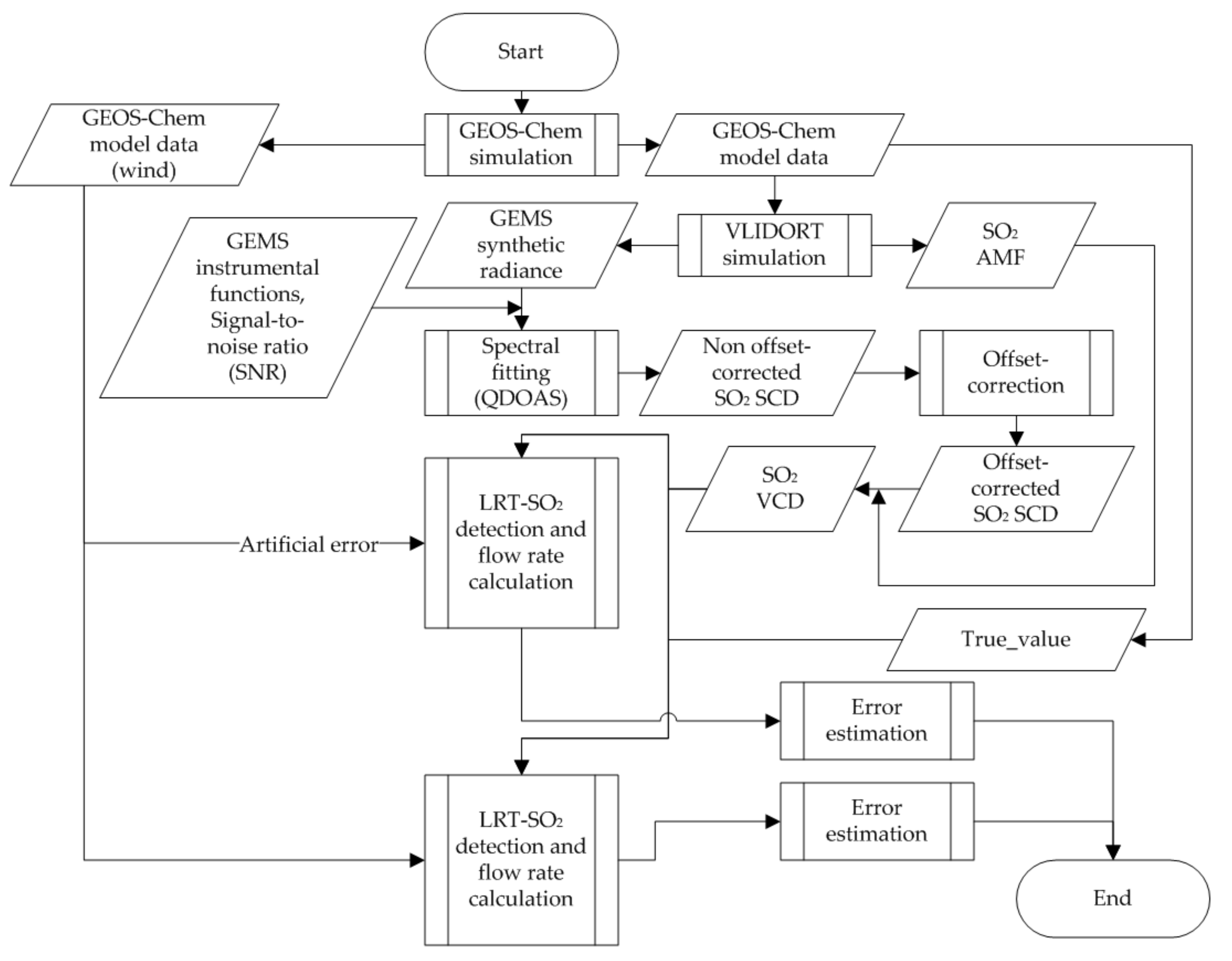
Figure 1 shows each step of the present study. We generated the GEMS synthetic radiances using the RTM (VLIDORT v2.6 [48]) and GEOS-Chem model [49] data. The SO₂ air mass factor (AMF) was also calculated with the RTM simulation. The SO₂ SCD retrieved from these GEMS synthetic radiances and the calculated (modeled) SO₂ AMF were used to retrieve the SO₂ VCDs. Thus, we focus on the SO₂ SCD retrieval error in this present study. AMF is another source of uncertainty in SO₂ VCD retrieval using the DOAS method [50]. The effect of AMF uncertainty was not accounted for in this study but will be considered in a separate study. To estimate the effect of GEMS SO₂ AMF uncertainties on the calculation of LRT-SO₂ flow rate, we first need to quantify the uncertainty of GEMS SO₂ AMF. To quantify the uncertainty of GEMS SO₂ AMF, the uncertainties and errors in the input data (most of which are GEMS L2 products), such as aerosol optical properties, aerosol layer height, cloud fraction, cloud pressure, surface reflectance, ozone column, and SO₂ vertical profile, which are used to calculate the GEMS SO₂ AMF, should be estimated. However, uncertainties and errors of the input data, most of which are GEMS L2 products, have not been evaluated. Therefore, the effect of GEMS SO₂ AMF uncertainty on the calculation of LRT-SO₂ flow rate can be investigated in a separate study once the uncertainties and errors of GEMS L2 products, which are used to calculate GEMS SO₂ AMF are quantified. That is, we considered that the SO₂ SCD relative error was equal to the SO₂ VCD relative error. We calculated the SO₂ VCD error from the difference between the retrieved and true SO₂ VCDs. The GEMS synthetic radiances were convoluted with GEMS instrumental functions [47,51]. The SO₂ SCDs were retrieved from these GEMS synthetic radiances. Thus, differences between true SO₂ SCDs and retrieved SO₂ SCDs can occur owing to the effects of GEMS instrumental functions and noise, and SCD error caused by the performance of SO₂ retrieval. The details of the SO₂ SCD retrieval method are described in Section 2.4. Here, the true SO₂ SCD and AMF were calculated directly from the RTM simulation. Having retrieved the SO₂ VCDs from the synthetic radiances and quantified the error, we used the SO₂ VCDs to detect the LRT-SO₂ event and to calculate the flow rate of the SO₂. Finally, the uncertainty associated with the LRT-SO₂ flow rate was estimated based on the validation datasets using the GEOS-Chem data. The method used to calculate the uncertainty of the LRT-SO₂ flow rate is described in Section 2.4.

2.1. GEOS-Chem

We used a 3-D global CTM GEOS-Chem [49] (www.geos-chem.org, accessed on 3 August 2021) to provide hourly trace gases (SO₂, HCHO, NO₂, and O₃) and aerosol concentrations to RTM simulations for generating the GEMS synthetic radiances. The GEOS-Chem output was also used in the validation of flow rate calculation as the true value. GEOS-Chem version 12.3.0 driven by the Goddard Earth Observation System-Forward Processing (GEOS-FP) assimilated meteorological fields at 0.25° × 0.3125° horizontal resolution and 47 vertical layers (from surface to ~0.01 hPa) were used. Nested simulations over a custom defined domain (110°E–140°E, 20°N–50°N) were conducted using boundary conditions from a GEOS-Chem global simulation at 2° × 2.5° resolution. For anthropogenic emissions inventory, we used version KORUSv2 [52] developed by Konkuk University to support the Korea–United States Air Quality (KORUS-AQ) campaign [53]. For other settings, including natural emissions and model chemistry, we refer the reader to Lee et al. [54].

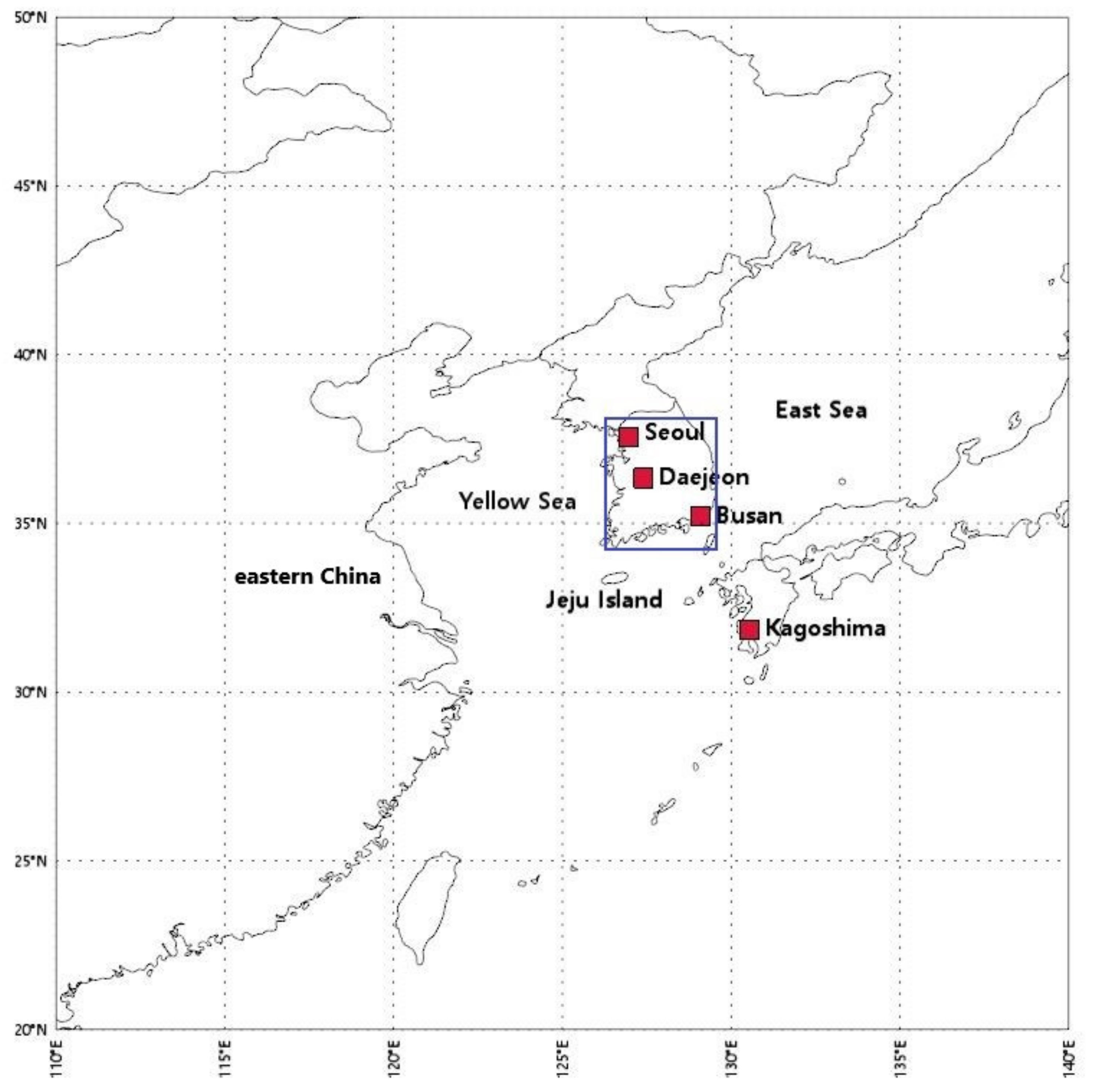
To calculate the true LRT-SO₂ flow rate, we performed the GEOS-Chem simulation twice: with and without anthropogenic and natural emissions over the blue rectangle in Figure 2. This blue rectangle defines the receptor area where the LRT-SO₂ flow rate was estimated. The output from the simulation with full emissions was used as input to calculate the flow rate of SO₂. The output from the simulation without emissions over the blue rectangle was used to calculate the true LRT-SO₂ flow rate. We then estimated the errors associated with the calculated SO₂ flow rate. We quantified the SO₂ flow rate errors via a comparison between the true LRT-SO₂ flow rate and the calculated LRT-SO₂ flow rate.

2.2. OMI Level 2 SO₂

We used the OMI Level 2 (L2) SO₂ data from the domain area shown in Figure 2 to define the SO₂ column contributed by regional emissions (i.e., the background SO₂ amount). The OMI sensor is onboard the Earth Observing System (EOS)/Aura satellite, which was launched on 15 July 2004 and flies in a sun-synchronous polar orbit with an equator-crossing time of around 13:45 local time (LT) in the ascending node at an altitude of 705 km altitude [43]. We used the OMI L2 SO₂ column data, which were produced from an updated algorithm in 2015. These OMI data are archived at NASA’s Goddard Earth Sciences Data and Information Services Center (GES DISC). They consist of daily global L2 gridded (L2G) SO₂ data from the OMI, having a spectral resolution of 0.45 nm in the UV band and a spatial resolution of 13 × 24 km (along track × cross track) at nadir [43].

2.3. HYSPLIT Backward Trajectory Model

We defined an LRT-SO₂ event at a receptor pixel when the contribution of LRT-SO₂ from the source areas was considered to have changed the atmospheric SO₂ level in the receptor pixel. We used the HYSPLIT backward trajectory model (version 4.9), developed by the National Oceanic and Atmospheric Administration, Air Resources Laboratory (NOAA/ARL) [45], to identify the travel route of the air mass. We used the National Centers for Environmental Prediction/National Center for Atmospheric Research (NCEP/NCAR) reanalysis meteorological data for the HYSPLIT backward trajectory simulation. Air mass backward trajectories from each receptor site were calculated every 0.1 km above ground level (agl) for each event. Stohl [55] reported that HYSPLIT simulated trajectory endpoints have uncertainties of ~20% of the travel distance. However, another study [56] reported that these uncertainties could exceed 20% in the first few time steps. Given a short average transport time of 2 days in the present study, we set the random errors of wind data to range from −15% to +15% for estimating the effect of wind data uncertainty on LRT-SO₂ flow rate calculation.

2.4. Method

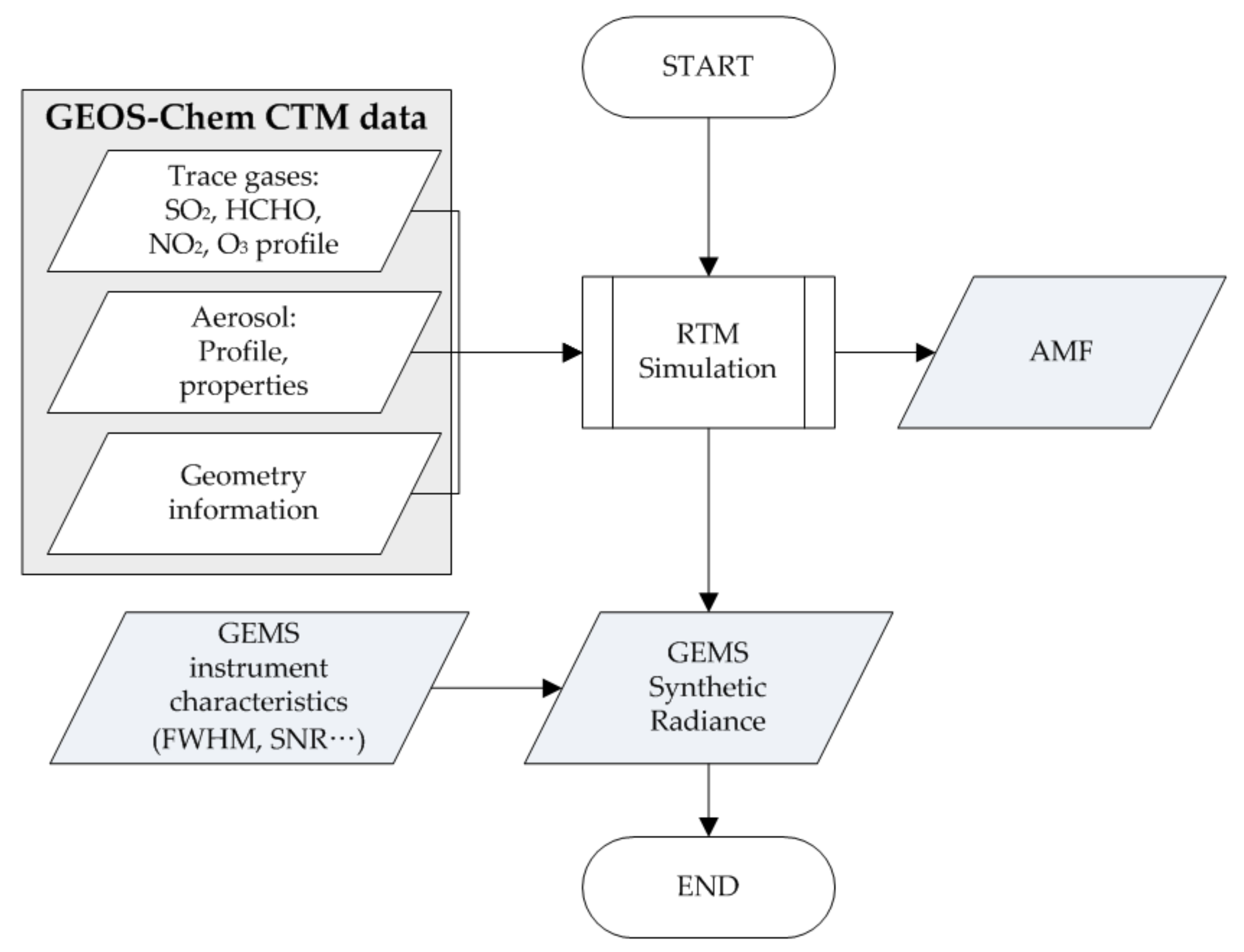
To quantify the uncertainties associated with the retrieval of the SO₂ flow rate, the SO₂ VCD was retrieved from the generated synthetic radiance by entering simple, known SO₂ in the CTM, and the flow rate was then calculated using the retrieved SO₂ VCD and known wind information. Figure 3 shows a flowchart of synthetic radiance generation using RTM (VLIDORT, v2.6) with inputs from the GEOS-Chem model, which was simulated with full emissions (see Section 2.1). The vertical profiles of trace gases, aerosol, pressure, and temperature data were obtained from GEOS-Chem. We also used the aerosol properties (aerosol peak height, single-scattering albedo, and aerosol type) and geometry information obtained from the GEOS-Chem. In the present study, we carried out instrument modeling according to the Observing System Simulation Experiment (OSSE) [50,51,57,58]. First, synthetic radiances were generated using VLIDORT from 310 to 326 nm with a 0.2 nm sampling resolution. Second, the generated synthetic radiances were convoluted with GEMS instrumental functions. Noise was added to the convoluted synthetic radiances to satisfy a signal-to-noise ratio (SNR) of 1440 according to Equation (1). The operational GEMS SO₂ retrieval algorithm present its product over either 2 × 2 or 4 × 4 pixels. However, an SNR of 1440 (4 × 4 pixels) was used in this present study because the GEOS-Chem model [49], which assimilated meteorological fields at 0.25° × 0.3125° (the spatial resolution of the assimilated field is approximately the same as 4 × 4 GEMS pixels) was used for the calculation of SO₂ flow rate. In this study, noise was added using the following equation [51,57,58]:

$${\mathrm{SNR}}_{\mathrm{i}}\left(\mathsf{\lambda }\right)={\mathrm{SNR}}_{\mathrm{a}}\times \sqrt{\frac{{\mathrm{I}}_{\mathrm{i}}\left(\mathsf{\lambda }\right)}{{\mathrm{I}}_{\mathrm{a}}}}$$

(1)

where ${\mathrm{SNR}}_{\mathrm{i}}\left(\mathsf{\lambda }\right)$ and ${\mathrm{I}}_{\mathrm{i}}\left(\mathsf{\lambda }\right)$ are the ith SNR and radiance at wavelength $\mathsf{\lambda }$, respectively; ${\mathrm{I}}_{\mathrm{a}}$ is the average value of all synthetic radiances from 310 to 326 nm; and ${\mathrm{SNR}}_{\mathrm{a}}$ is its corresponding SNR.

We adopted the GEMS SO₂ operational algorithm to retrieve SO₂ SCDs in this present study because this study aimed to determine whether it is possible to calculate the SO₂ flow rate over the GEMS measurement domain using the GEMS SO₂ products. The GEMS SO₂ operational algorithm [47,59], which requires SO₂ retrieval over a whole GEMS measurement domain within 30 min, is a combined algorithm of Principal Component Analysis (PCA) [44] and multi-window DOAS [60]. Currently, PCA is the operational SO₂ retrieval algorithm in the OMI and the Ozone Mapping and Profiler Suite (OMPS) [61]. Multi-window DOAS was used as the operational SO₂ retrieval algorithm in TROPOMI [60]. However, PCA cannot be used for GEMS synthetic radiances in the present study because PCs, which are extracted from synthetic radiances, tend to be influenced by the SO₂ absorption effect. Once PCs influenced by the SO₂ absorption effect are used to retrieve SO₂ SCDs, the SO₂ SCDs cannot be retrieved from the synthetic radiances using the SO₂ contaminated PCs and SO₂ absorption cross-section. Therefore, in the present study, we used the multi-window DOAS method, which is used partly as the GEMS SO₂ operational algorithm, to quantify SO₂ SCD retrieval error.

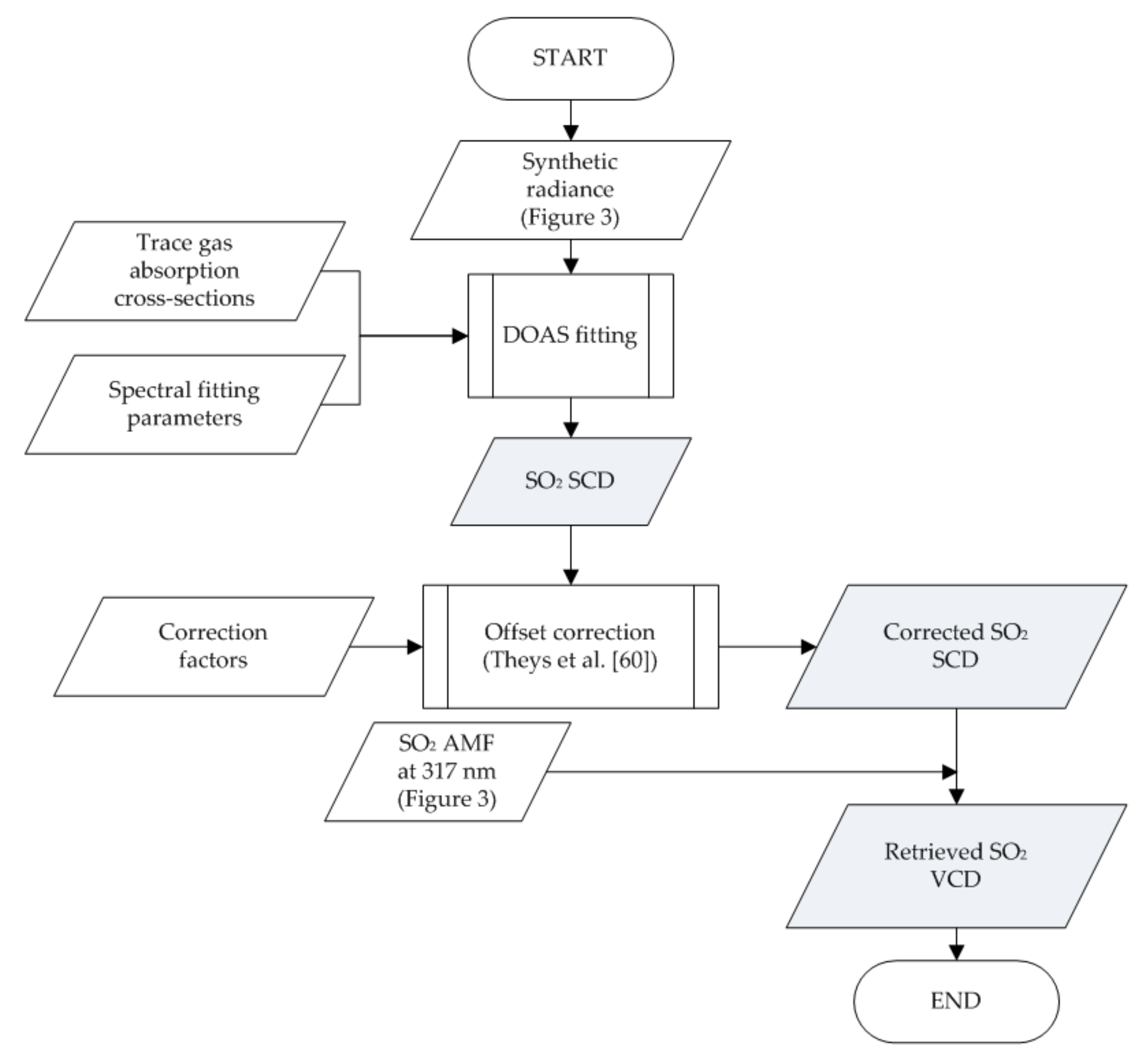
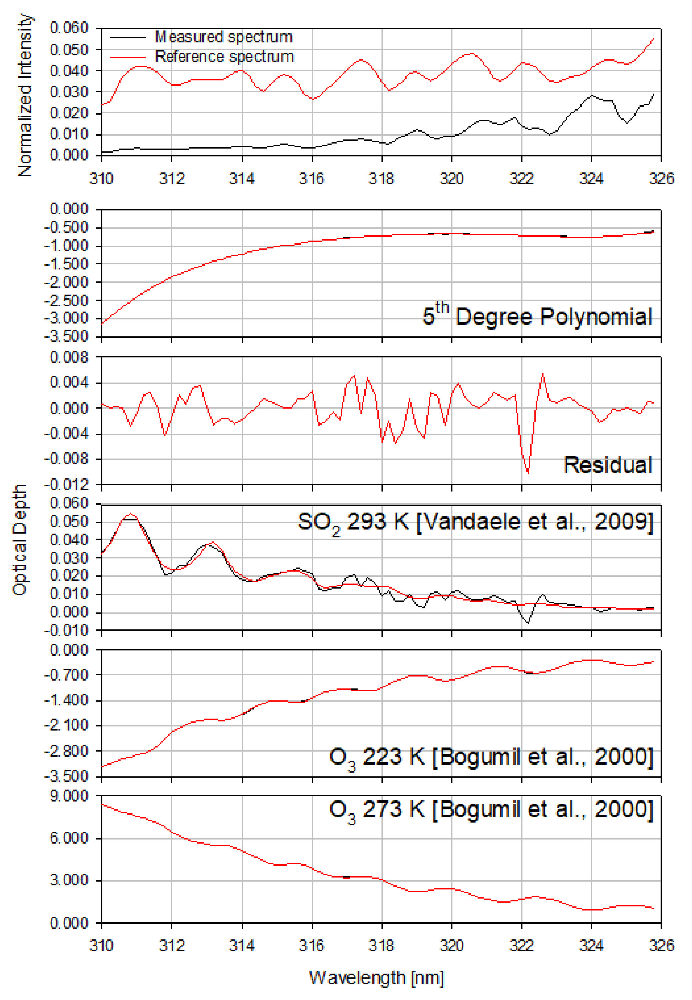
We used SO₂ VCDs retrieved from the synthetic radiances to determine the pixels affected by LRT-SO₂ and to calculate the LRT-SO₂ flow rate. Figure 4 summarizes the SO₂ VCD retrieval from the synthetic radiances. In general, we used the DOAS technique [62] to retrieve the SO₂ SCD, which is the total amount of SO₂ integrated over the light path length, which is affected by absorption and scattering in the atmosphere and reflected by the surface between the sun and a satellite sensor. The optical density fitting was carried out over the wavelength range (310–326 nm) using the QDOAS software [63]. This spectral interval, which includes a strong SO₂ absorption band that peaks between about 310 and 313 nm, was found to have the smallest spectral fitting residual (optical density of residual = 0.021). We used the SO₂ and O₃ cross-sections to retrieve the SO₂ SCD. In addition, we used the same cross sections to generate the synthetic radiance as were used to retrieve the SO₂ SCD. The SO₂ absorption cross-section is from Vandaele et al. [64]. The O₃ (223 K and 293 K) absorption cross-sections are from Bogumil et al. [65]. We used a fifth-order polynomial to account for Rayleigh and Mie scattering. All absorption cross-sections were convolved using the GEMS slit function. The SO₂ and O₃ spectra were I_o-corrected using the QDOAS software. Figure 5 shows an example of DOAS spectral fitting for SO₂ SCD retrieval in the Kagoshima volcanic area, Japan at 06:00 (UTC) 09 April 2016.

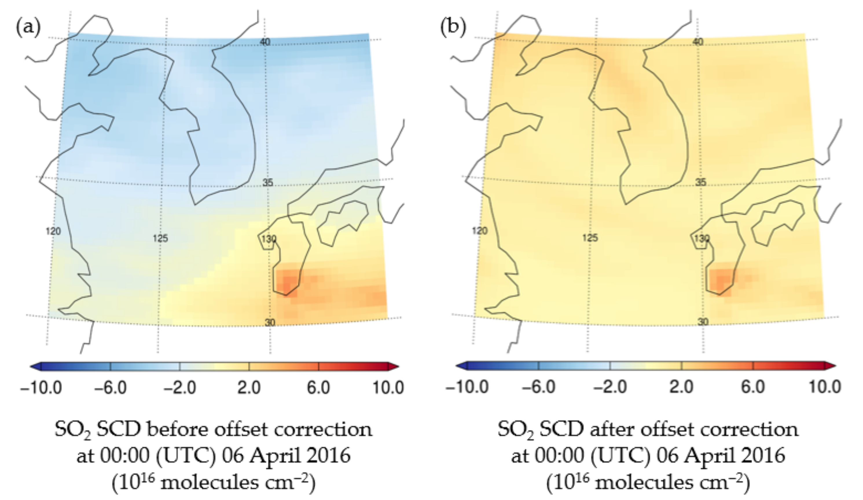
The retrieved SO₂ SCDs were offset-corrected [60]. Figure 6 shows examples of the SO₂ SCD distributions at 00:00 (UTC) 06 April 2016 over the receptor area. Figure 6a,b shows the SO₂ SCDs before and after the offset correction, respectively. The biases shown in Figure 10 can be attributed to the ozone effect, which is a well-known, common problem with most algorithms that retrieve SO₂ SCDs from UV sensors onboard satellites [57]. As shown in Figure 6, the SO₂ SCD before ozone correction (the so-called “offset correction”) is much smaller than the SO₂ SCD after offset correction. Therefore, the SO₂ SCDs contained a negative bias owing to this ozone effect. The negative biases of the SO₂ SCDs due to the ozone effect can be partly reduced after the offset correction. Thus, the negative biases presented in Figure 10 are part of the SO₂ SCD retrieval error due to the ozone effect. However, the magnitude of these biases can vary depending on the SO₂ retrieval algorithm used.

The AMF was calculated using the VLIDORT RTM, and the same inputs were used to simulate the synthetic radiances. The AMFs were used to convert the offset-corrected SO₂ SCDs into SO₂ VCDs (AMF = SCD/VCD). The AMF was calculated at 317 nm, which is the center of the fitting window. The error of the retrieved SO₂ VCD also contained an uncertainty, as a 2% difference was calculated between SO₂ AMF at 317 and 318 nm. Differences between true SO₂ VCDs and retrieved SO₂ VCDs can be attributed mainly to the SO₂ SCD retrieval error and partly to the uncertainty of AMF caused by the GEMS SO₂ AMF calculated at a center wavelength. The scattering weight, ${\mathsf{\omega }}^{\prime }\left(\mathrm{z}\right)$, and the shape factor, ${{\mathrm{S}}^{\prime }}_{\mathrm{z}}$(z), in each layer can be expresses as the AMF, as follows [66]:

$$\mathrm{AMF}={\mathrm{AMF}}_{\mathrm{G}}{{\displaystyle \int }}_0^{\infty }{\mathsf{\omega }}^{\prime }\left(\mathrm{z}\right){{\mathrm{S}}^{\prime }}_{\mathrm{z}}\left(\mathrm{z}\right)\mathrm{dz}$$

(2)

where ${\mathrm{AMF}}_{\mathrm{G}}$ is the geometric AMF. A detailed description of VLIDORT and the AMF calculations can be found in Spurr and Christi [48].

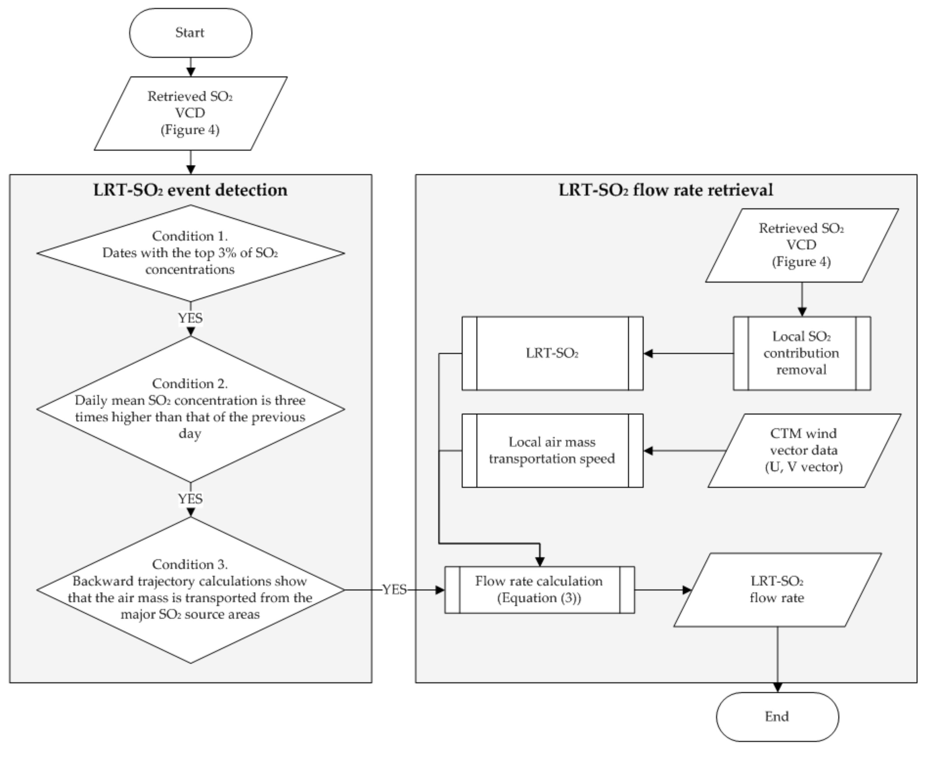
Figure 7 shows the methods used to determine the LRT-SO₂ events and to calculate the SO₂ flow rate. First, we categorized the LRT-SO₂ events as periods when SO₂ levels in a pixel were increased by LRT-SO₂ from continental Asia or volcanic areas. Three conditions (left grey rectangle in Figure 7) were used to categorize the pixel with the LRT-SO₂ event. A detailed description of these conditions can be found in Park et al. [42]. For this study, we used the SO₂ column densities obtained from the CTM simulation for condition 1, whereas surface SO₂ concentrations from in situ measurements were used by Park et al. [42]. Second, we calculated the flow rate of the LRT-SO₂ over the pixel with the LRT-SO₂ event, as shown in Figure 7 (grey rectangle on the right-hand side).

$$\begin{gathered} {\mathrm{SO}}_2 \mathrm{flow} \mathrm{rate}=\mathrm{LRT}\text{-}{\mathrm{SO}}_2 \mathrm{column} \left(\mathsf{\alpha }\right) \times \mathrm{average}\mathrm{transportation}\mathrm{speed}\mathrm{of}\mathrm{the} \\ \mathrm{air}\mathrm{mass} \left(\mathsf{\beta }\right)\times \mathrm{GEOS}\text{-}\mathrm{Chem}\mathrm{grid}\mathrm{length} \end{gathered}$$

(3)

The LRT-SO₂ flow rate was calculated using Equation (3), where $\mathsf{\alpha }$ and $\mathsf{\beta }$ denote the LRT-SO₂ column and the average transportation speed of the air mass, respectively. To calculate the LRT-SO₂ column amount ($\mathsf{\alpha }$), the contribution from local SO₂ emissions needs to be quantitatively estimated. A previous study used in situ ground measurements to quantify SO₂ from local contributions [42] because continuously monitored SO₂ data are useful in quantifying the locally contributed SO₂. However, in the present study, we used the SO₂ VCD obtained from the OMI L2 SO₂ data to quantify SO₂ amount from local sources as in situ ground measurement data are not available for all pixels where the LRT-SO₂ flow rate needs to be calculated. The local SO₂ VCD was calculated by averaging the OMI SO₂ column data that were available for the 15 days before and after each event date, excluding the data measured on the event date. We excluded the data measured on the event date because it is possible that calculated local SO₂ VCD is overestimated owing to the LRT-SO₂ on the event date. We calculated LRT-SO₂ column based on Equation (4) as follows:

$$\mathsf{\alpha }={\mathrm{SO}}_2\mathrm{VCD}-{\mathrm{SO}}_2{\mathrm{VCD}}_{\mathrm{local}}$$

(4)

where $\mathsf{\alpha }$ is the LRT-SO₂ column (i.e., the SO₂ column at each synthetic radiance pixel due to LRT-SO₂), and SO₂VCD and SO₂VCD_local represent the SO₂ VCD measured for each pixel and SO₂ VCD from local contributions, respectively. The mean value of $\mathsf{\alpha }$ (1.3 × 10¹⁶ molecules cm⁻²) was much larger than 2.5 × 10¹⁵ molecules cm⁻², which is the sum of the mean SO₂VCD_local and the standard deviation of SO₂VCD_local (4.0 × 10¹⁴ molecules cm⁻²). This present study used Equation (4) to estimate LRT-SO₂, as suggested by a previous study [42]. However, Equation (4) may underestimate the LRT-SO₂ column when LRT-SO₂ is affected by the local SO₂ column and may overestimate the LRT-SO₂ column when the local SO₂ column is underestimated compared with a real local SO₂ column.

We also calculated the local air mass transportation speed ($\mathsf{\beta }$) by averaging the local transportation speeds of the air masses. Air mass transportation speeds were calculated from the U and V vectors used for the GEOS-Chem simulation. We calculated the air mass transport speed for cases of volcanic and anthropogenic emission. We calculated the air mass transport speed for volcanic emission case using the U and V vectors of the air masses that originated from surface to ~0.01 hPa. On the other hand, we calculated the air mass transport speed using the U and V vectors of the air masses that originated within the PBL in the source area and were transported to the receptor area because the anthropogenic SO₂ is assumed to be located mostly within the PBL in the source areas [67,68]. We used the PBL data that were simulated by GEOS-Chem. We also used the OMI L2 SO₂ data to define the SO₂ source areas. The areas with high SO₂ emissions reported in previous studies [1,69,70] and the areas with a high SO₂ column in the OMI L2 SO₂ data were coincident, and these areas were defined as the source areas. A more detailed description of this procedure can be found in Park et al. [42].

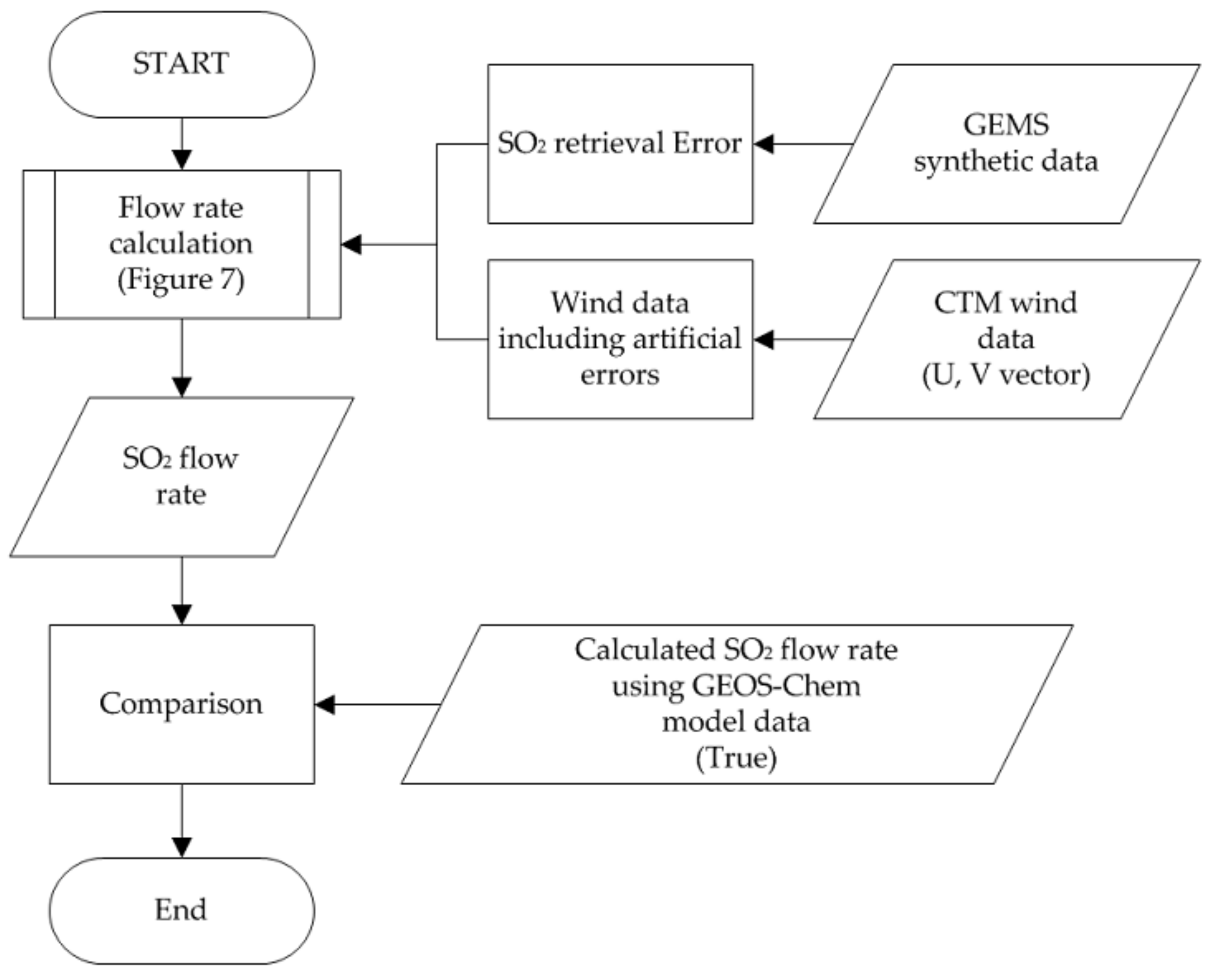
We investigated the uncertainties in the LRT-SO₂ flow rate under the SNR of 1440 condition and for various wind data with random errors ranging from −15% to +15% (Figure 8). The absolute percentage difference (APD) between the LRT-SO₂ flow rate and the true LRT-SO₂ flow rate was calculated as follows:

$$\mathrm{APD}=\frac{\left({\mathrm{True} \mathrm{flow} \mathrm{rate} \mathrm{of} \mathrm{SO}}_2-{ \mathrm{Retreived} \mathrm{flow} \mathrm{rate} \mathrm{of} \mathrm{SO}}_2\right)}{{\mathrm{True} \mathrm{flow} \mathrm{rate} \mathrm{of} \mathrm{SO}}_2}\times 100$$

(5)

where the true flow rate of SO₂ is calculated as the LRT flow rate of SO₂ based on GEOS-Chem SO₂ profile data. In addition, the retrieved flow rate of SO₂ is calculated as the LRT flow rate of SO₂ based on SO₂ VCDs, which are retrieved as shown in Figure 4.

3. Results

Table 1. SO₂ long-range transportation events.

Event No.	Date	Emission Source
1	06–14 April 2016	Anthropogenic and volcanic sources
2	17–25 April 2016	Volcanic source
3	25–30 April 2016	Volcanic source
4	03–11 July 2016	Volcanic source
5	17–25 July 2016	Anthropogenic and volcanic sources
6	20–30 October 2016	Anthropogenic and volcanic sources

lists the LRT-SO₂ events and the event dates determined using the three conditions shown in Figure 7. All events in Table 1 represent high-SO₂ events when LRT-SO₂ reaches the Korean Peninsula or the sea around the Korean Peninsula (e.g., the Yellow Sea, East Sea, or South Sea). In addition, all events in Table 1 were affected by either a combination of anthropogenic emissions and volcanic eruptions, or just volcanic SO₂ emissions. Mount Shindake, which is located in Japan (Kagoshima), erupted on 29 May 2015 and has continued to erupt since then. Events 1, 5, and 6 were additionally affected by anthropogenic sources because SO₂ emitted from the Asian continent was transported to the Korean Peninsula by the trade winds.

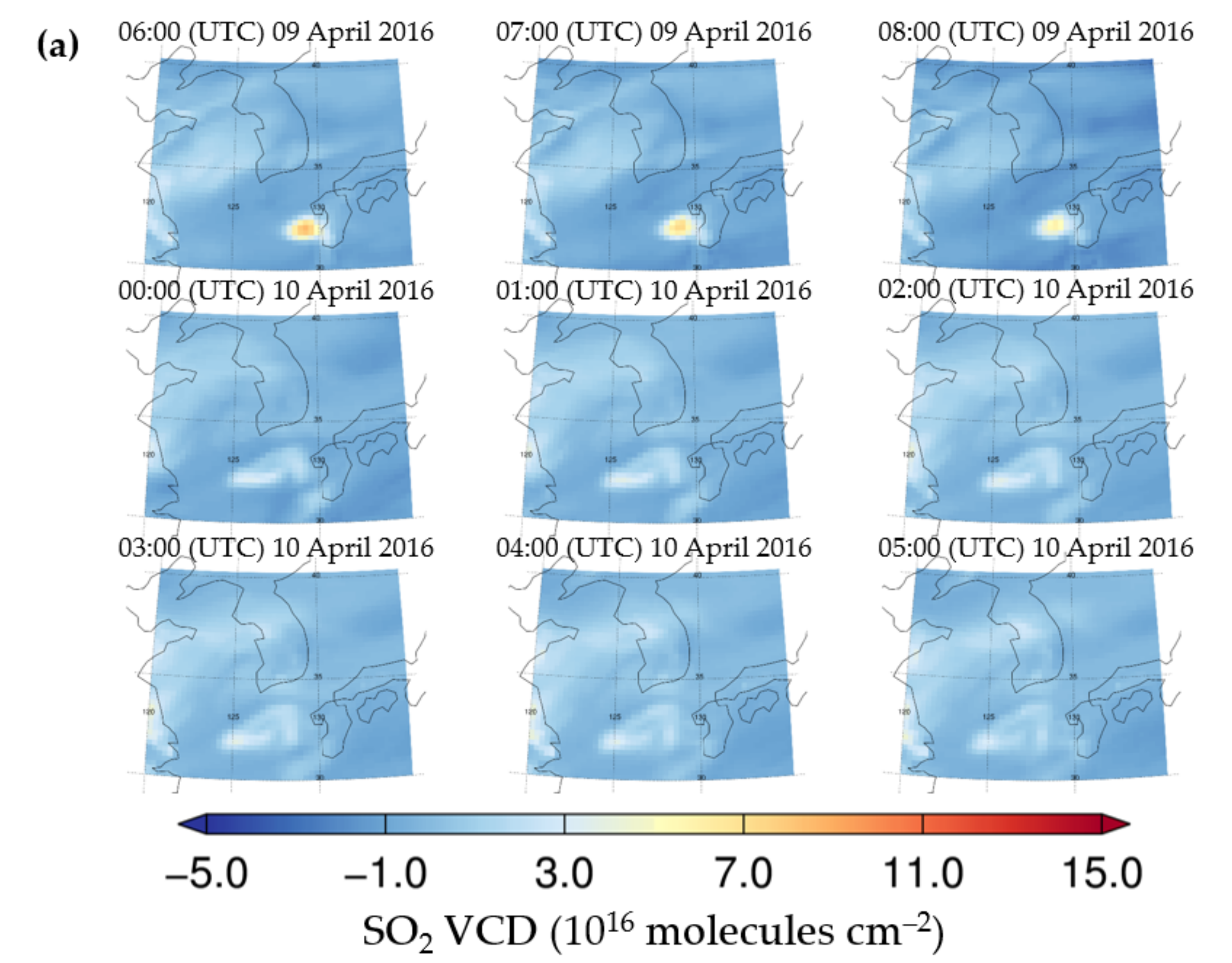
Once the GEMS synthetic radiances were produced for the event dates in Table 1 (Figure 3), the SO₂ VCDs were retrieved from these radiances according to the DOAS technique described in Figure 4. Then, the LRT-SO₂ flow rate over the Korean Peninsula was calculated based on the algorithms (shown in Figure 7) with the inputs of the retrieved SO₂ VCDs and wind data that were used to run GEOS-Chem. Figure 9a shows the SO₂ VCD retrieved from the GEMS synthetic radiance (SO₂ VCD_Retrieved) on 09–10 April 2016, and Figure 9b shows the SO₂ VCD simulated from the GEOS-Chem (SO₂ VCD_True) on the same date. Figure 9 shows examples of SO₂ VCD_Retrieved and SO₂ VCD_True for event 1 in Table 1. Figure 9 shows high SO₂ VCDs over eastern China and Kagoshima in Japan.

Figure 9 shows how the volcanic SO₂ plume from Kagoshima was transported to the southern part of the Korean Peninsula. The maximum (average) SO₂ VCD_Retrieved and SO₂ VCD_True values over the southern part of the Korean Peninsula were 0.2 (0.2) and 1.2 (1.1) × 10¹⁶ molecules cm⁻², respectively, before the volcanic SO₂ plume arrived. However, the maximum (average) SO₂ VCD_Retrieved and SO₂ VCD_True values over the southern part of the Korean Peninsula were 6.2 (4.1) and 14.1 (11.4) × 10¹⁶ molecules cm⁻², respectively, after the arrival of the volcanic SO₂ plume. In addition, LRT-SO₂ from Asia to the Korean Peninsula was well-detected. In terms of anthropogenic SO₂ effects, the maximum (average) SO₂ VCD_Retrieved and SO₂ VCD_True over the Korean Peninsula (near Seoul) were 0.2 (0.1) and 2.4 (2.1) × 10¹⁶ molecules cm⁻², respectively, before the anthropogenic SO₂ plume was transported from eastern China. However, the maximum (average) SO₂ VCD_Retrieved and SO₂ VCD_True for Seoul were 2.1 (1.9) and 5.3 (4.6) × 10¹⁶ molecules cm⁻², respectively, when the anthropogenic SO₂ plume arrived from eastern China.

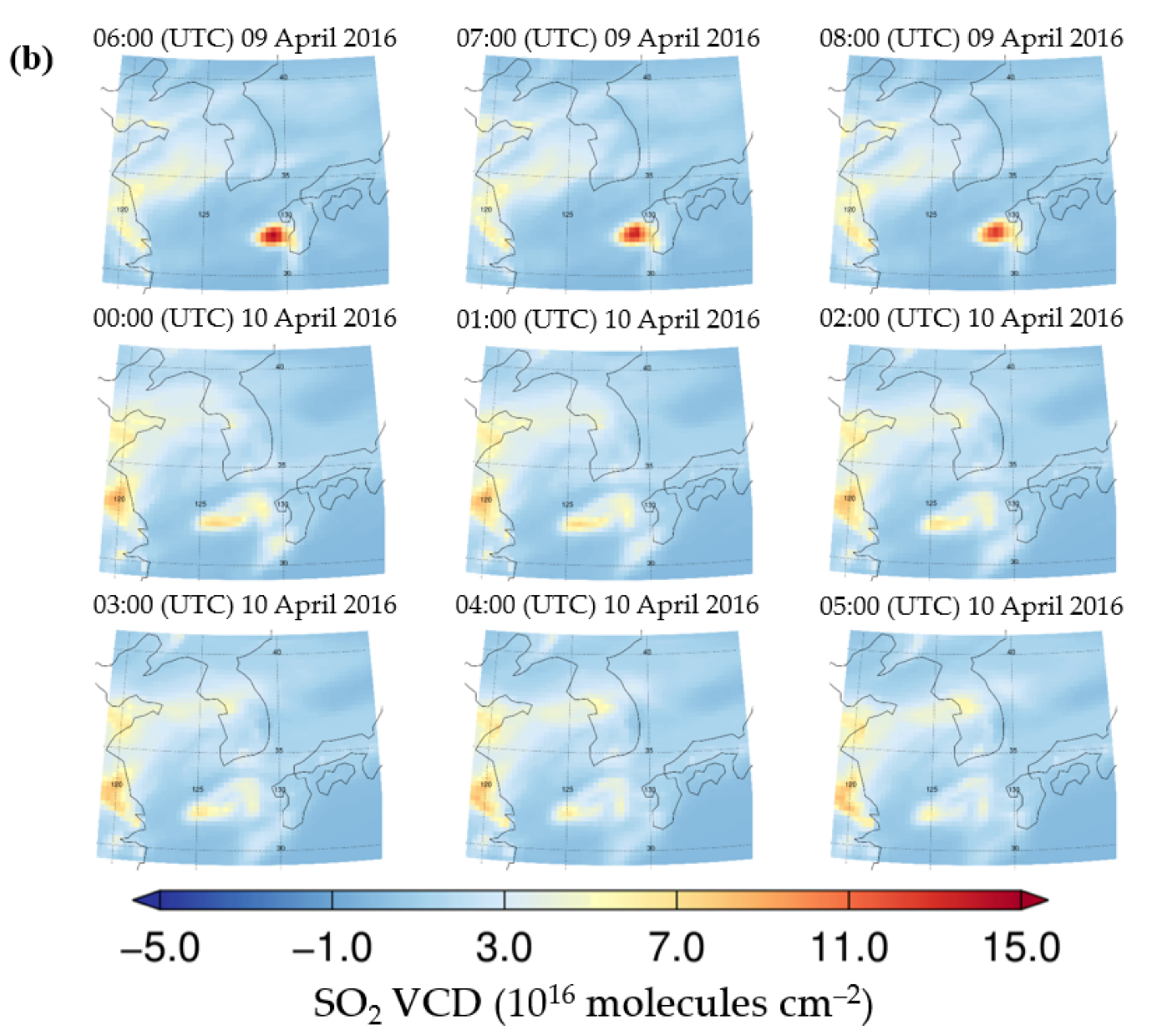
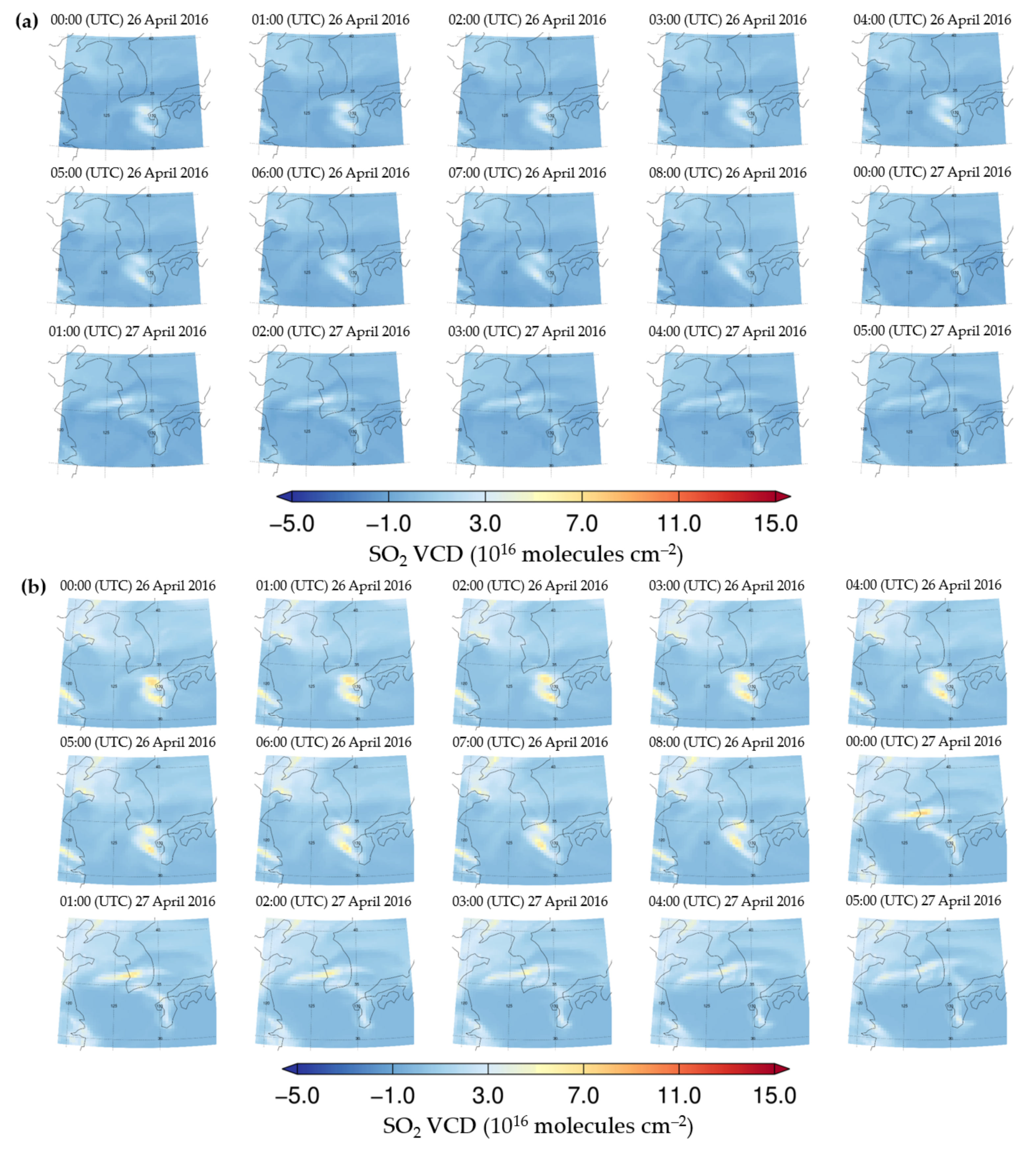
Figure 10 shows the SO₂ VCD_Retrieved and SO₂ VCD_True from event 3 in Table 1. High-SO₂ VCDs occurred over eastern China and Kagoshima in Japan, and a volcanic SO₂ plume from Kagoshima was transported across several cities in Korea (Busan, Daejeon, and Seoul). Before the volcanic SO₂ plume reached these cities, the maximum (average) SO₂ VCD_Retrieved and SO₂ VCD_True levels were −0.2 (−0.6) and 0.4 (0.1) × 10¹⁶ molecules cm⁻² over Busan, −0.4 (−0.5) and 1.1 (0.6) × 10¹⁶ molecules cm⁻² in Daejeon, and −0.7 (−0.9) and 2.1 (1.3) × 10¹⁶ molecules cm⁻² in Seoul. The maximum (average) SO₂ VCD_Retrieved and SO₂ VCD_True values were 3.2 (2.7) and 6.5 (5.9) × 10¹⁶ molecules cm⁻² over Busan, 4.1 (3.8) and 6.8 (6.1) × 10¹⁶ molecules cm⁻² over Daejeon, and 2.8 (2.5) and 3.9 (3.4) × 10¹⁶ molecules cm⁻² over Seoul after the volcanic SO₂ plume reached them.

The spatial distribution of SO₂ VCD_Retrieved agrees well with that of the true SO₂ VCDs in Figure 9 and Figure 10. However, the value of SO₂ VCD_Retrieved tends to underestimate SO₂ VCD_True. It should be remembered that the SO₂ VCD error represents the SO₂ SCD retrieval error in this study. The SO₂ SCD retrieval error is the difference between the true and retrieved SO₂ SCD values (see Section 2 for a more detailed explanation). 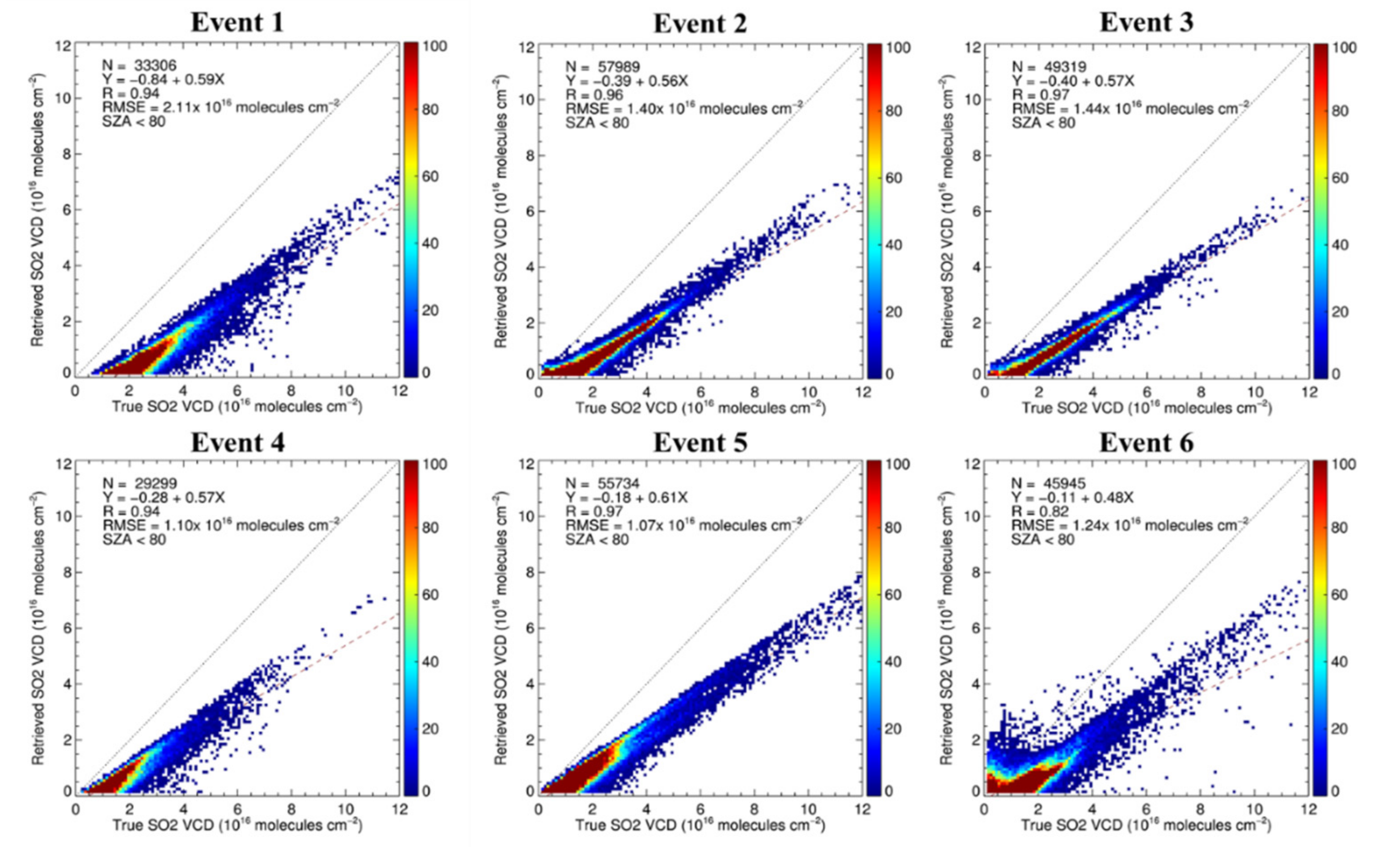To investigate the uncertainty of the flow rate of LRT-SO₂, which is calculated using SO₂ VCD_Retrieved, the accuracy of the SO₂ VCD_Retrieved obtained in this study needs to be quantified. To understand the accuracy of SO₂ VCD_Retrieved, we compared the true SO₂ VCD values with those retrieved for all events in Figure 11. For the comparisons, we selected pixels with (1) a range of VCDs from 5.0 × 10¹⁴ to 1.2 × 10¹⁷ molecules cm⁻², (2) a DOAS fitting residual < $\pm$0.001, (3) an SCD error < 20%, and (4) a solar zenith angle < 70°. The scatter plots (Figure 11) show the correlation between the retrieved SO₂ VCD_Retrieved and SO₂ VCD_True. On all of these plots, the dashed red line and dotted black line represent the regression line and 1:1 line, respectively. The colors and color bar in Figure 11 indicate the data number for the values.

Table 2. Correlation between SO₂ VCD_True and SO₂ VCD_Retrieved.

Event No.	R	Slope	Intercept	$\mathbf{RMSE} (\times {10}^{16}\mathbf{Molecules}{\mathrm{cm}}^{-2})$
1	0.94	0.59	−0.84	2.11
2	0.96	0.56	−0.39	1.40
3	0.97	0.57	−0.40	1.44
4	0.94	0.57	−0.28	1.10
5	0.97	0.61	−0.18	1.07
6	0.82	0.48	–0.11	1.24

lists the correlation coefficient (R), slope, intercept, and root mean square error (RMSE) between true SO₂ VCDs and those retrieved for each event.

Figure 11 and Table 2 show the correlation between the SO₂ VCD_Retrieved and SO₂ VCD_True. The correlation coefficient (R) varies from 0.82 to 0.97, and the slope varies from 0.48 to 0.61. The RMSE values range from 1.10 to 2.11 × 10¹⁶ molecules cm⁻², which equates to a retrieval uncertainty of about 40% to 80% of the retrieved SO₂ column densities. In particular, for event 6, the correlation coefficient and slope show poor agreement between the SO₂ VCD_Retrieved and SO₂ VCD_True, which is associated with the low magnitude of SO₂ VCD in comparison with those for other events. The average SO₂ VCD_True values range from 2.1 to 3.2 × 10¹⁶ molecules cm⁻² for events 1 through 5, but the value is 1.8 × 10¹⁶ molecules cm⁻² for event 6, which implies that lower SO₂ VCD_True values lead to an increase in the percentage uncertainty associated with the retrieved SO₂ VCD.

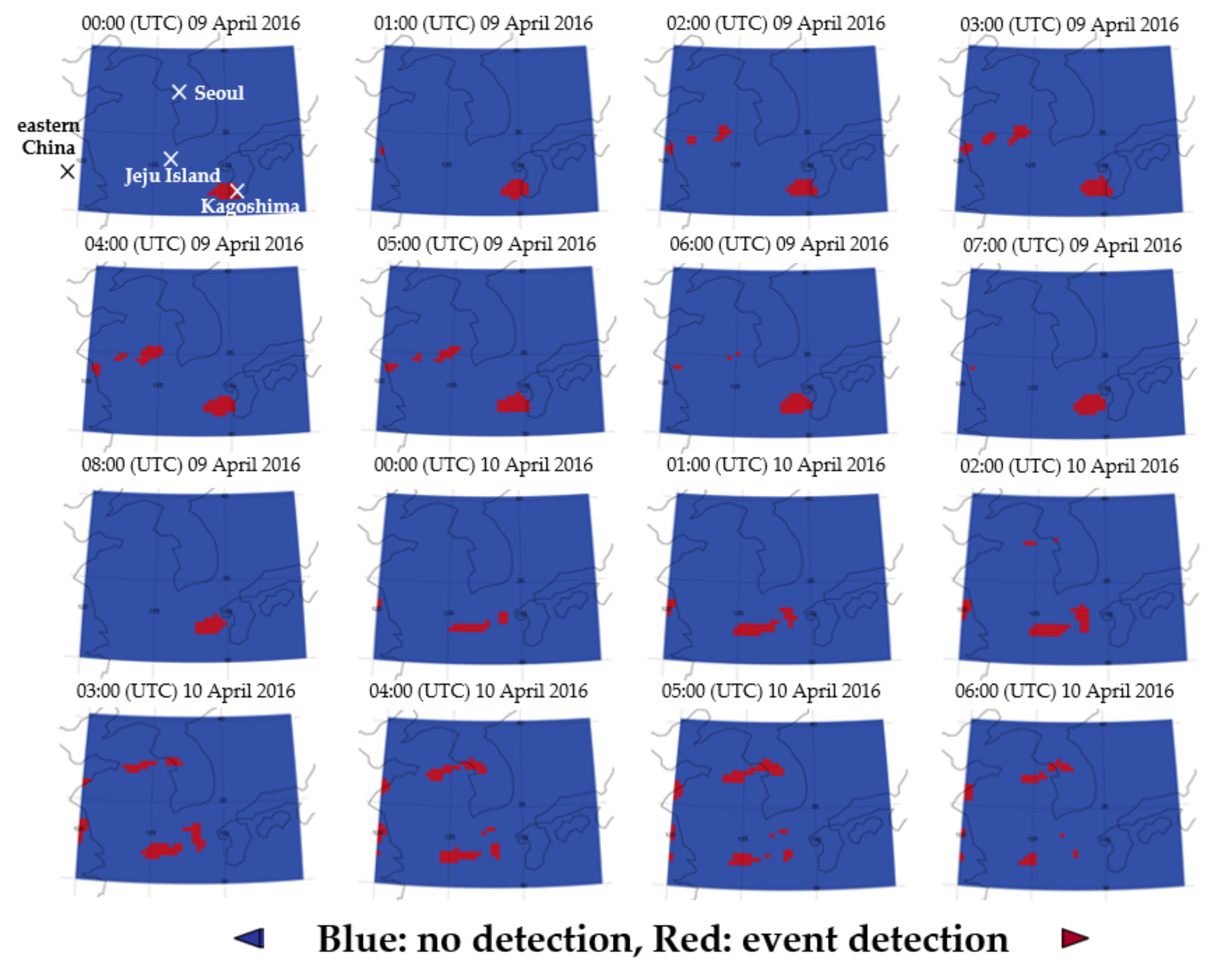
Once SO₂ VCDs were obtained from the GEMS synthetic radiances and their error was calculated (Figure 11 and Table 2), the SO₂ VCDs were used to detect the LRT-SO₂ events and to calculate the flow rate of the SO₂. Figure 12 shows the detection of the LRT-SO₂ plume for the period 09–10 April 2016. The red shading represents the pixels that were affected by LRT-SO₂ according to the method described in Figure 7, and the blue shading indicates those not affected by LRT-SO₂. The three conditions outlined in Figure 7 were applied to determine the pixels affected by LRT-SO₂ for event 1 (9–10 April 2016) using the retrieved SO₂ VCDs. The red pixels show northward movement of the SO₂ plume that originated from the Kagoshima volcanic area in Japan. The LRT-SO₂ was found over Kagoshima at 00:00 (UTC) on 9 April 2016 and near Jeju Island at 03:00 (UTC) on 10 April 2016. In addition to the volcanic SO₂ transport during event 1, SO₂ transport from eastern China was also found over the Yellow Ocean between 01:00 and 06:00 (UTC) on 9 April 2016 and over the middle of the Korean Peninsula between 02:00 and 06:00 (UTC) on 10 April 2016, as shown in Figure 12.

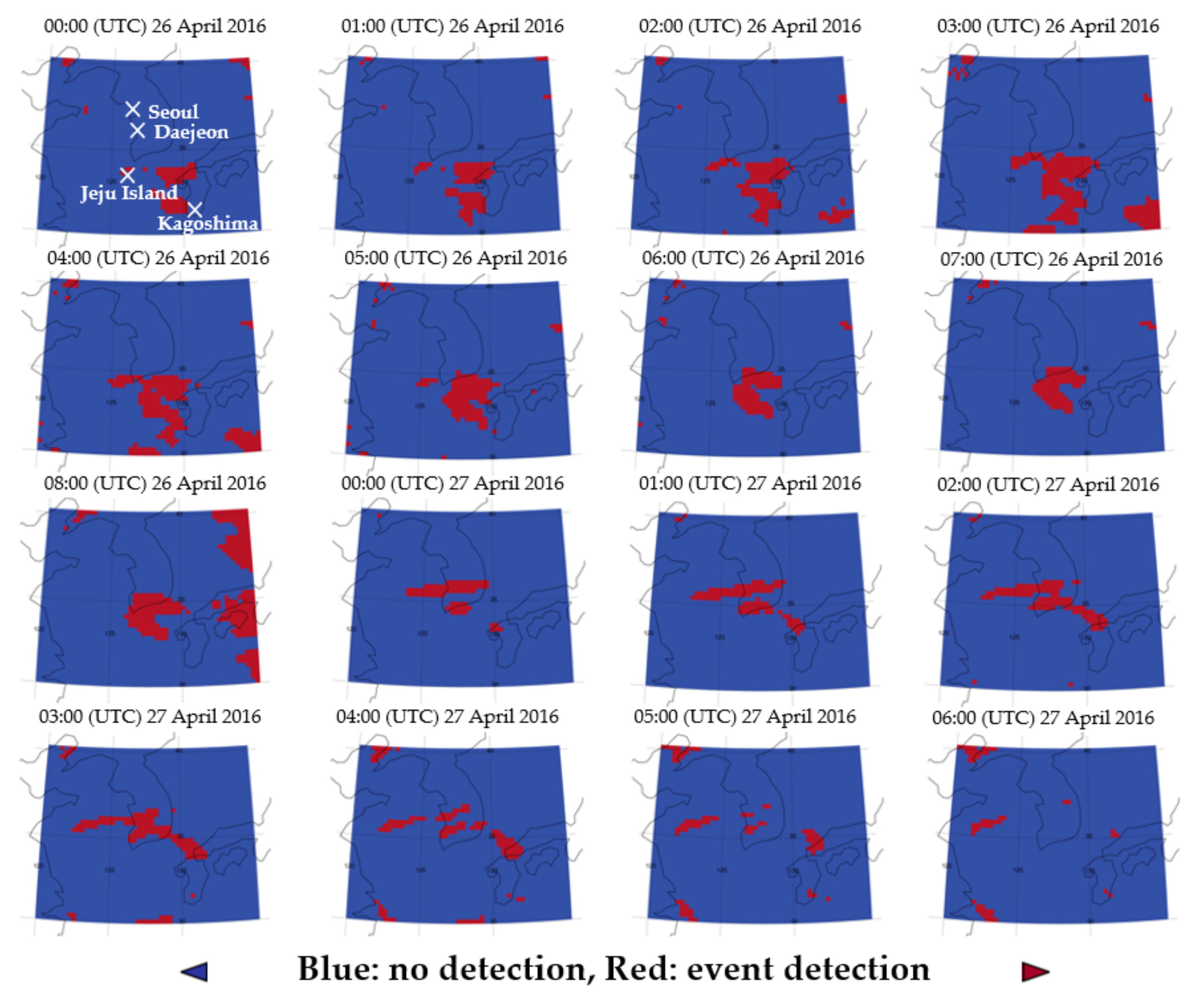
Figure 13 shows the pixels affected by LRT-SO₂ throughout event 3. The pixels affected by transported volcanic SO₂ were also determined by the method described in Figure 7. Volcanic SO₂ plumes emitted from Kagoshima reached the southern part of the Korean Peninsula at 05:00 (UTC) on 26 April 2016. Volcanic SO₂ plumes were present over the Korean Peninsula from 05:00 (UTC) on 26 April 2016 to 04:00 (UTC) on 27 April 2016. The volcanic SO₂ VCD_Retrieved value was 7.2 × 10¹⁶ molecules cm⁻² over Kagoshima (the volcanic SO₂ source area) at 05:00 (UTC) on 26 April 2016 when the plume began to affect the Korean Peninsula. The volcanic SO₂ VCD_Retrieved was 5.3 × 10¹⁶ molecules cm⁻² over Daejeon at 04:00 (UTC) on 27 April 2016.

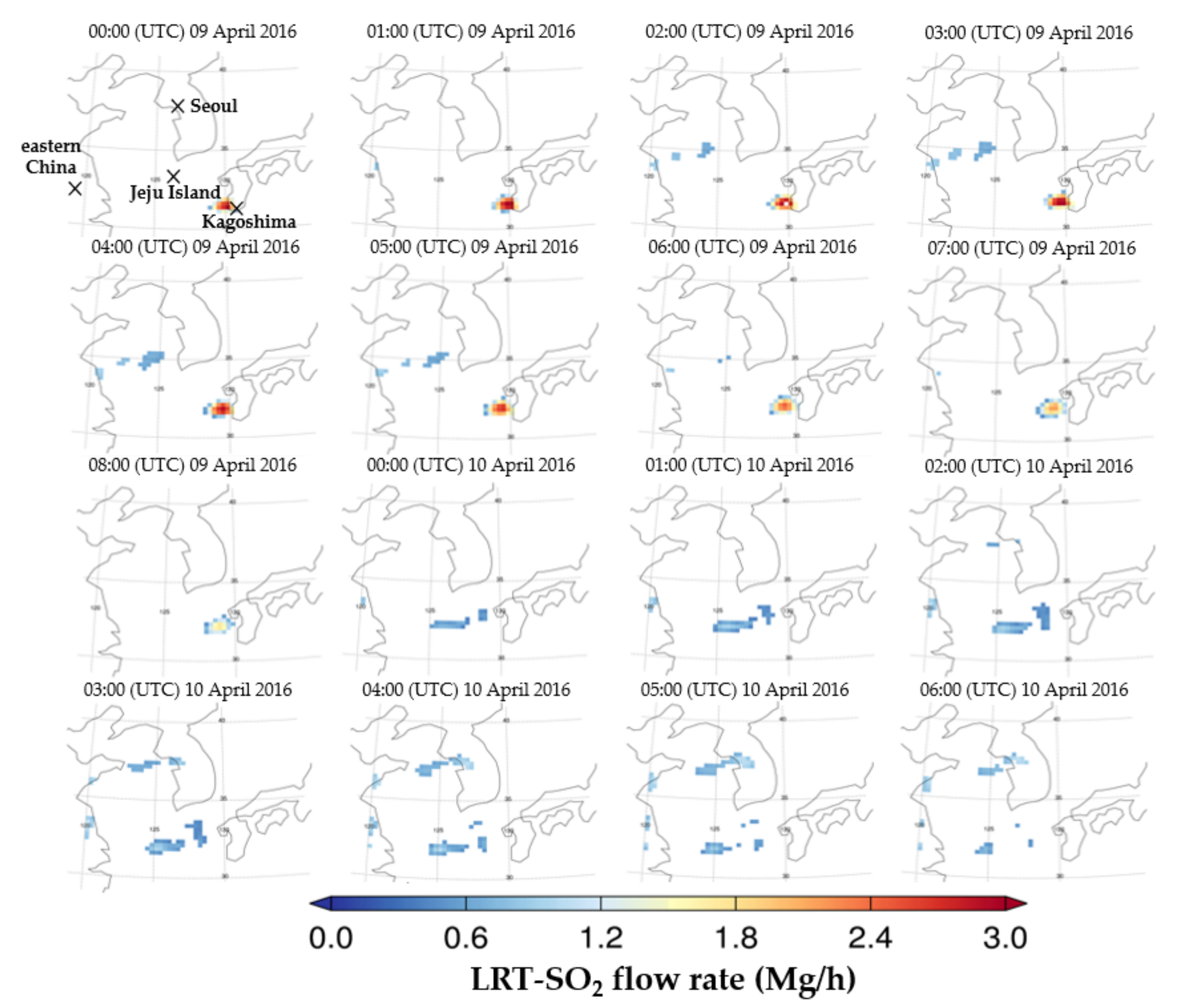
The LRT-SO₂ flow rates were calculated using Equation (3) and the method described in Figure 7. Figure 14 shows the SO₂ flow rates calculated for the pixels that were determined to be affected by LRT-SO₂ during event 1 (Figure 12). As shown in Figure 12 and Figure 14, the transported SO₂ plumes were well-captured and observed to move from the Kagoshima volcanic area in Japan to the South Ocean of the Korean Peninsula and from industrial areas of eastern China to west of the Korean Peninsula. In the case of the LRT-SO₂ from the Kagoshima volcanic area, the average, maximum, and minimum values of the SO₂ flow rate over the southern part of the Korean Peninsula (near Jeju Island) were calculated to be 1.4, 2.1, and 1.1 Mg/h, respectively. For the SO₂ transported from industrial areas of eastern China, the corresponding values over the Yellow Sea were 0.32, 0.51, and 0.38 Mg/h, respectively. To evaluate the accuracy of these calculated SO₂ flow rates, we compared our SO₂ flow rate estimates with the true SO₂ flow rates. The true SO₂ flow rate was calculated using the method described in Section 2 and Figure 7. For the volcanic SO₂ plume, the average of the calculated SO₂ flow rate (true flow rate) over the southern Korean Peninsula (near Jeju Island) was 1.1 (2.3) Mg/h whereas it was 0.8 (1.8) Mg/h over the Yellow Ocean for the anthropogenic SO₂ plume from eastern China. The difference between the average calculated SO₂ flow rates and the true rates was 3.1 and 1.2 Mg/h for the volcanic and anthropogenic SO₂ plumes, respectively.

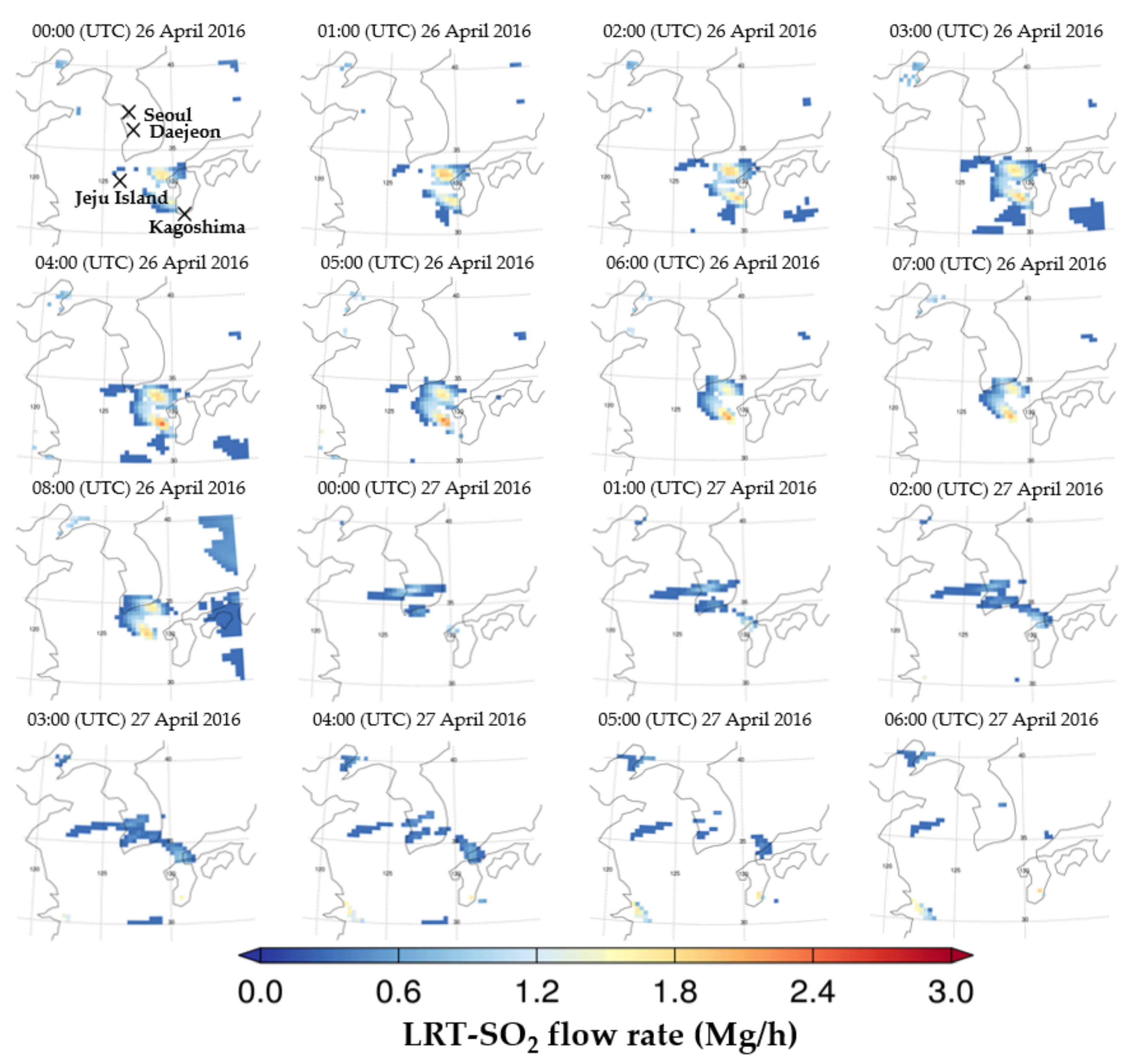
Figure 15 shows the SO₂ flow rates calculated for the pixels that were determined to be affected by the LRT-SO₂ during event 3 (Figure 13). We found a general decrease in LRT-SO₂ flow rates with distance from the volcanic SO₂ source region. The calculated LRT-SO₂ flow rates (true flow rate) for pixels defined as being affected by long-range transportation was 2.3 (3.7) Mg/h over the Kagoshima region (03:00 (UTC) 26 April 2016), 1.1 (2.8) Mg/h over Jeju (07:00 (UTC) 26 April 2016), and 0.8 (2.1) Mg/h over Daejeon (01:00 (UTC) 27 April 2016). In the case of Daejeon, SO₂ VCD_Retrieved increased from 0.3 × 10¹⁶ molecules cm⁻² on 26 April 2016 (01:00 UTC), which was before the SO₂ LRT event, to 2.1 × 10¹⁶ molecules cm⁻² on 27 April 2016 (01:00 UTC), when the Kagoshima volcanic SO₂ had just arrived.

The maximum, minimum, and average LRT-SO₂ flow rates during event 3 were 1.89, 0.13, and 0.94 Mg/h, respectively, whereas those for the true SO₂ flow rates were 4.43, 0.14, and 0.96 Mg/h, respectively. The differences between the two sets of values were caused mostly by the SO₂ SCD retrieval error associated with the DOAS spectral fitting method. However, uncertainties in the SO₂ flow rate calculation are also created by uncertainties in the wind data, SO₂ AMF, and SO₂ SCD. The uncertainties in the SO₂ flow rate calculations were evaluated by accounting for uncertainties in the wind data and SO₂ SCD and are discussed in the next section.

Error Estimation

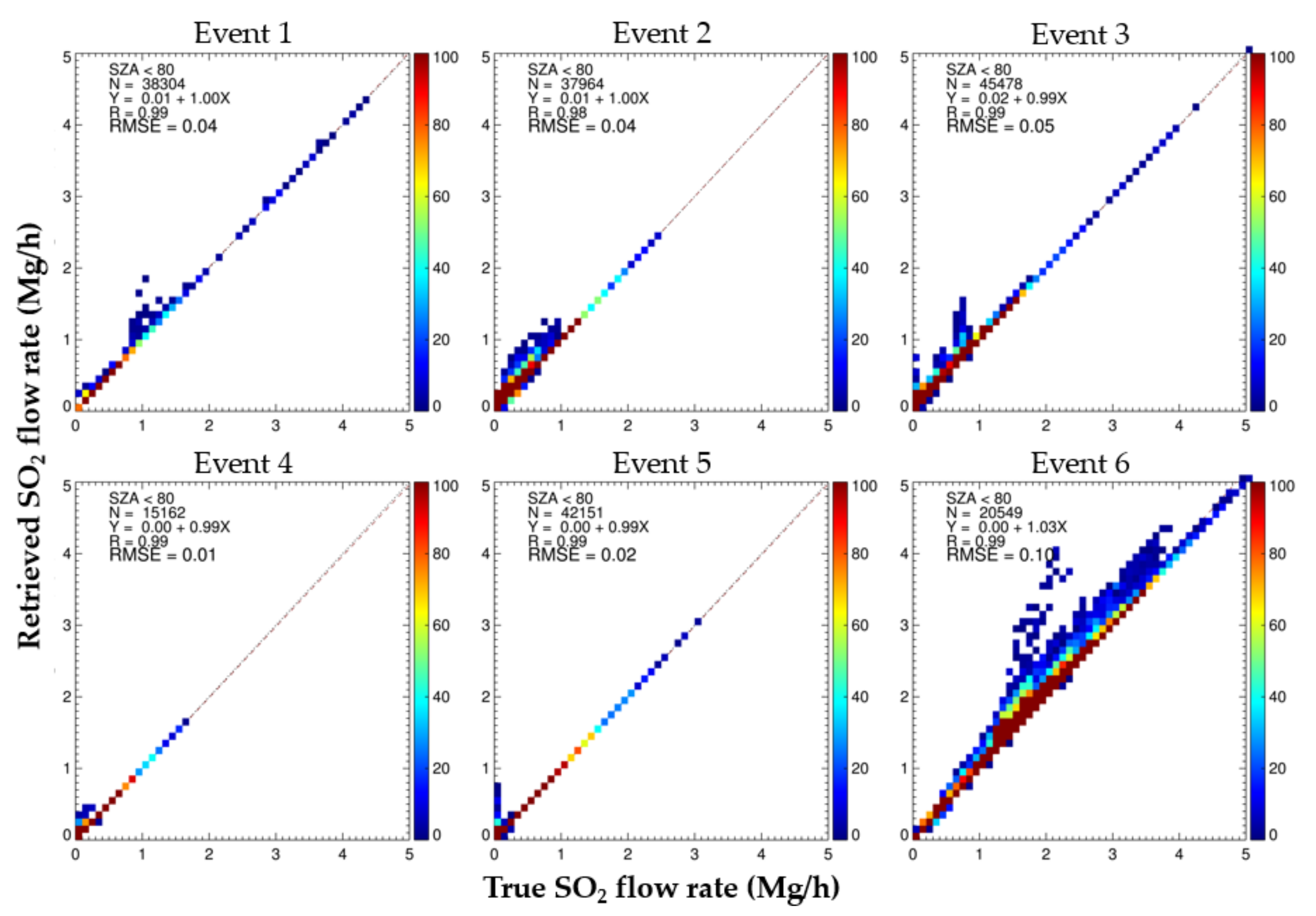
We compared our calculated SO₂ flow rates with those of the true ones to estimate the magnitude of the errors associated with the calculated values. The true SO₂ flow rates were calculated using the method shown in Figure 8, with inputs of true wind data and true SO₂ column density. The true SO₂ column densities do not contain a retrieval error or the contribution of the SO₂ emissions from the receptor areas because they were simulated using the GEOS-Chem SO₂ column with the SO₂ emission off in the receptor region on the Korean Peninsula. We evaluated the accuracy of the LRT-SO₂ flow rates calculated under the conditions of the true SO₂ VCDs and wind data. The correlation coefficient, slope, and intercept between the calculated flow rates and the true values ranged from 0.98 to 0.99, from 0.99 to 1.03, and from 0.00 to 0.02 Mg/h, respectively (Figure 16). The SO₂ emissions from the Korean Peninsula contributed 0.01–0.10 Mg/h of the RMSE in the SO₂ flow rate calculation (

Table 3. Statistical analysis of the true SO₂ flow rates and those calculated under the presence of no errors in the SO₂ retrieval and no uncertainty in wind data.

No Error Condition
Event No.	R	Slope	Intercept	RMSE (Mg/h)	Average Flow Rate (Standard Deviation)
					True	Retrieved
1	0.99	1.00	0.01	0.04	1.29 ($\pm$0.79)	1.34 ($\pm$0.82)
2	0.98	1.00	0.01	0.04	0.73 ($\pm$0.48)	0.84 ($\pm$0.45)
3	0.99	0.99	0.02	0.05	0.96 ($\pm$0.46)	0.96 ($\pm$0.45)
4	0.99	0.99	0.00	0.01	0.13 ($\pm$0.12)	0.14 ($\pm$0.12)
5	0.99	0.99	0.00	0.02	0.38 ($\pm$0.36)	0.38 ($\pm$0.35)
6	0.99	1.03	0.00	0.10	3.58 ($\pm$0.48)	3.58 ($\pm$0.48)

). For all events except event 2, we obtained a difference of less than 8% between the true SO₂ flow rate and those calculated under the conditions of no errors in the SO₂ retrieval and wind data. These small differences can be attributed to uncertainties in the SO₂ flow rate calculation method, such as uncertainty in the local SO₂ column removal (Figure 7 and Equation (4)).

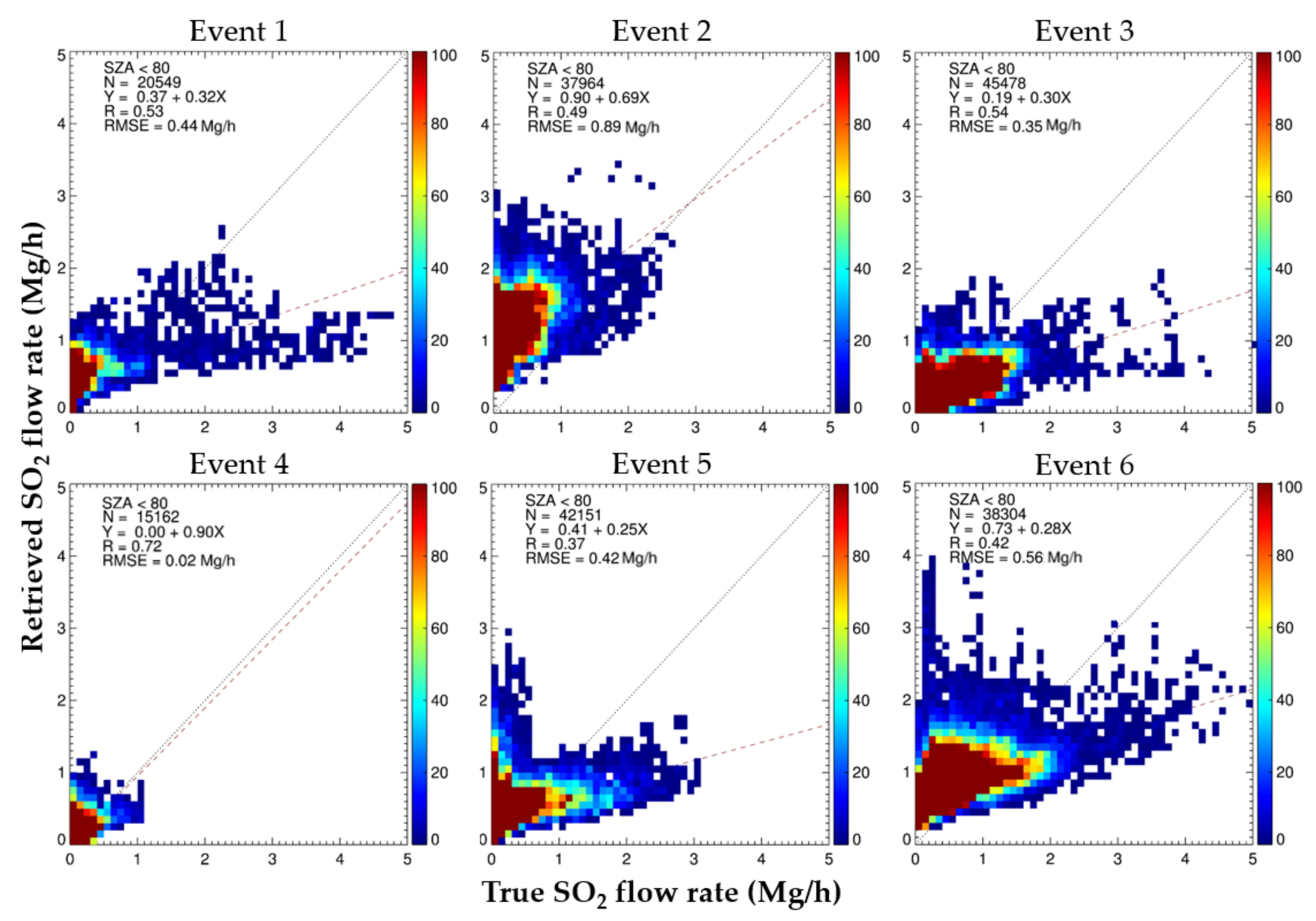
We investigated the uncertainties in LRT-SO₂ flow rate retrieval associated with both the GEMS SO₂ L2 data and the wind data. The calculated SO₂ flow rates in Figure 17 were obtained using the true wind data, which were used as the inputs for the GEOS-Chem simulation, as well as the SO₂ column densities retrieved from the GEMS synthetic radiances, and these account for the SNR of 1440 for the SO₂ spectral fitting wavelength range. The SO₂ flow rates were calculated for a solar zenith angle of less than 70°. The calculated SO₂ flow rates in Figure 17 contain GEMS retrieval errors only. Figure 17 shows the correlation between the true SO₂ flow rates and those calculated under the conditions of the GEMS SO₂ retrieval error but with no errors in wind data for all events in Table 1. The slope and intercept between the true and calculated SO₂ flow rates range from 0.23 to 0.63 and from 0.09 to 0.82 Mg/h, respectively. As shown in Figure 17, the RMSE for all events ranges from 0.14 to 0.79 Mg/h and the minimum and maximum R values are 0.37 and 0.72, respectively. These statistics of the SO₂ flow rate calculation are mostly due to errors in the SO₂ SCD retrieval from GEMS.

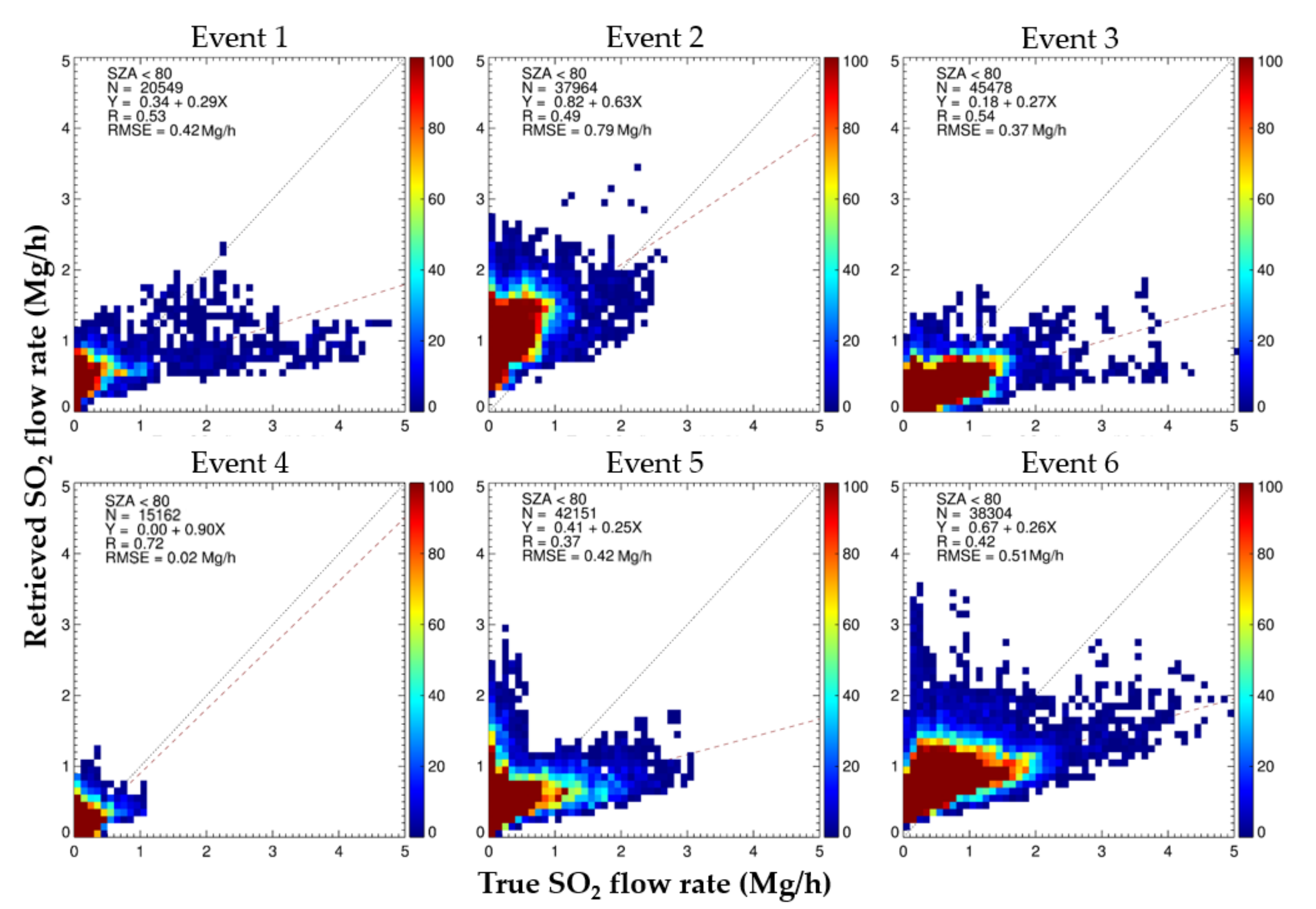
Figure 18 shows the correlation between the true SO₂ flow rates and those calculated in the presence of uncertainties in both wind data and SO₂ VCD retrievals for all events in Table 1. To evaluate the effects of wind data uncertainty in addition to that associated with the SO₂ VCD retrievals from the GEMS synthetic radiances, we calculated the SO₂ flow rates using the wind data used in the GEOS-Chem simulations but with random errors added that ranged from −15% to 15%, following Stohl [55]. When the uncertainties in both the SO₂ VCD retrieval and wind data were present, the errors in the SO₂ flow rates were much larger than those generated from only the SO₂ VCD retrieval error. The average true SO₂ flow rates (standard deviation) and those calculated in the presence of both the SO₂ VCD retrieval error and wind data uncertainty were 1.17 ($\pm$0.44) and 1.04 ($\pm$0.70) Mg/h, respectively. As shown in Figure 18, the RMSE for all events ranges from 0.02 to 0.79 Mg/h. The minimum and maximum R values between the true SO₂ flow rates and those calculated were 0.37 and 0.72, respectively.

Table 4. Statistical analysis of the true SO₂ flow rates and those calculated under the presence of the SO₂ retrieval error from the GEMS synthetic radiances and no uncertainty in wind data.

GEMS Instrument Characteristics + SNR Of 1440
Event No.	R	Slope	Intercept	RMSE (Mg/h)	Average Flow Rate (Standard Deviation)
					True	Retrieved
1	0.53	0.29	0.34	0.42	1.29 ($\pm$0.79)	0.98 ($\pm$0.91)
2	0.49	0.63	0.82	0.79	0.73 ($\pm$0.48)	0.62 ($\pm$0.56)
3	0.54	0.27	0.18	0.37	0.96 ($\pm$0.46)	0.72 ($\pm$0.57)
4	0.72	0.90	0.00	0.02	0.13 ($\pm$0.12)	0.11 ($\pm$0.13)
5	0.37	0.23	0.38	0.39	0.38 ($\pm$0.36)	0.29 ($\pm$0.41)
6	0.42	0.26	0.67	0.51	3.58 ($\pm$0.48)	2.99 ($\pm$0.95)

lists the R values, slope, intercept, and RMSE between the true LRT-SO₂ flow rate and calculated LRT-SO₂ flow rates in the presence of the GEMS SO₂ retrieval error and no uncertainty in wind data, whereas

Table 5. LRT-SO₂ flow rate uncertainties under the conditions of errors in both wind data and GEMS SO₂ retrieval.

GEMS Instrument Characteristics + SNR of 1440 + Meteorological Data Error
Event No.	R	Slope	Intercept	RMSE (Mg/H)	Average Flow Rate (Standard Deviation)
					True	Retrieved
1	0.53	0.32	0.37	0.44	1.29 ($\pm$0.79)	1.14 ($\pm$0.81)
2	0.49	0.69	0.90	0.89	0.73 ($\pm$0.48)	0.79 ($\pm$0.66)
3	0.54	0.30	0.19	0.35	0.96 ($\pm$0.46)	0.94 ($\pm$0.65)
4	0.72	0.90	0.00	0.02	0.13 ($\pm$0.12)	0.10 ($\pm$0.15)
5	0.37	0.25	0.41	0.42	0.38 ($\pm$0.36)	0.31 ($\pm$0.40)
6	0.42	0.28	0.73	0.56	3.58 ($\pm$0.48)	3.00 ($\pm$1.55)

shows the values in the presence of both the GEMS SO₂ retrieval error and uncertainty in the wind data. The R values in Figure 17 are similar to those in Figure 18. The correlation coefficients between the true and calculated SO₂ flow rates range from 0.37 to 0.72 in Figure 17 and from 0.37 to 0.72 in Figure 18. The differences in the slope, intercept, and RMSE values shown in Table 4 and Table 5 range from 0.0% to 11.1%, from 0.0% to 9.7%, and from 5.4% to 12.6%, respectively. In particular, when comparing Table 4 and Table 5, there is a large difference in the SO₂ flow rate calculation errors of event 2. The large SO₂ flow rate error for event 2 in Table 5 is due to the uncertainty ($\pm$15%) of the calculated transport speed. When LRT-SO₂ flow rate was calculated in the condition of an SNR of 1440 without wind data uncertainties, the RMSE and standard deviation ranged from 0.02 to 0.79 Mg h⁻¹ and ±0.13 to ±0.95 Mg h⁻¹, respectively, as shown in Figure 17 and Table 4. However, the LRT-SO₂ flow rate was calculated in the presence of both an SNR of 1440 and wind data uncertainties, with RMSE and standard deviation ranging from 0.02 to 0.89 Mg h⁻¹ and from ±0.15 to ±1.55 Mg h⁻¹, respectively, as shown in Figure 18 and Table 5. RMSE and standard deviation tended to slightly increase in the presence of an SNR of 1440 and wind data uncertainties compared with those in the presence of only an SNR of 1440. In this study, errors related to AMF were not accounted for in the GEMS SO₂ retrieval error. According to a previous study [50], the SO₂ AMF errors caused by uncertainties in aerosol properties and surface reflectance were calculated as being between 46% and 173.4%. We calculated the SO₂ flow rate error based on the SNR of 1440. However, spatial pixel-binning is required to enhance the SNR and to reduce the GEMS SO₂ retrieval error and the SO₂ flow rate calculation error.

4. Discussion

SO₂ is one of the less-reactive atmospheric gas species compared with other reactive trace gases, such as NO_x, OH, O₃, and HCHO, and it can last in the atmosphere for several days [31,32]. Thus, SO₂ is transported on the regional and global scales. Several studies [33,34,35] investigated LRT-SO₂. Hsu et al. [34] reported that the SO₂ plume emitted from anthropogenic sources in eastern China is transported to eastern Pacific Ocean. Li et al. [33] also showed that the SO₂ plume emitted from China is transported to northwestern Pacific Ocean. Both Li et al. [33] and Hsu et al. [34] used OMI SO₂ data to observe LRT-SO₂.

The transport of SO₂ emission from Dalaffilla volcano has also been well-detected and reported in a previous study [35] using the OMI SO₂ data. These studies used the satellite SO₂ data only for the detection of SO₂ plume transport. Park et al. [42] proposed a method to estimate LRT-SO₂ values using the daily OMI SO₂ column, in situ data, and the HYSPLIT model. This previous study contributed to flow rate estimates and the assessment of their uncertainties from source areas over northeast Asia and the northwestern Pacific at several receptor locations. Subsequently, the GEMS instrument was launched in February 2020, and it is now theoretically possible to estimate the hourly SO₂ flow rate. However, it is important to understand the effects of GEMS SO₂ SCD retrieval errors on these LRT-SO₂ flow rate estimates. In particular, UV hyperspectral sensors, including GEMS, are known to have poor sensitivity to surface SO₂ levels because of the strong interference by ozone absorption and the SNR over the spectral fitting window for surface SO₂ retrieval. In this study, we attempted to estimate the LRT-SO₂ flow rate based on the synthetic GEMS radiances for several anthropogenic and volcanic SO₂ events over the Korean Peninsula and surrounding areas. Errors in the LRT-SO₂ flow rate estimates were quantified and related to errors in the GEMS SO₂ SCD retrieval and wind data uncertainty for those events. Although uncertainties associated with the AMF calculations were not accounted for in this study, our simulations showed that the accuracy of the LRT-SO₂ flow rate estimates depends primarily on the GEMS SO₂ SCD retrieval errors, which are partly associated with the SNR of 1440 over the 310–326 nm band. The RMSE and standard deviation between the true LRT-SO₂ flow rate and calculated LRT-SO₂ flow rates are found to be increased slightly due to the wind data uncertainty. Thus, a larger SO₂ SCD retrieval error leads to a larger uncertainty in the LRT-SO₂ flow rate estimates. In the present study, the multi-window DOAS algorithm [59,60], which is used partly as the GEMS SO₂ operational algorithm [59], was used to quantify the SO₂ SCD retrieval error. However, there are still chances to reduce the SO₂ SCD retrieval error using other SO₂ retrieval algorithms although the GEMS operational algorithm requires fast retrieval within 30 min. Spatial pixel-binning can increase the GEMS radiance SNR, although it decreases the spatial resolution. An increased SNR can reduce the SO₂ SCD retrieval error, which eventually leads to an increase in SO₂ flow rate estimates.

5. Conclusions

We calculated LRT-SO₂ flow rates using hourly synthetic GEMS measurements over Northeast Asia. We retrieved the SO₂ VCD from the GEMS synthetic radiances using the multi-window DOAS algorithm. The SO₂ VCDs retrieved and the true SO₂ VCDs show ranges from −1.1 to 6.2 and from 0.4 to 14.1 × 10¹⁶ molecules cm⁻². In addition, the mean values of the SO₂ VCDs retrieved and the true SO₂ VCDs were calculated as 1.7 and 3.1 × 10¹⁶ molecules cm⁻², respectively. The retrieved SO₂ VCDs were compared with the true SO₂ VCDs calculated from the SO₂ vertical profile used as the input data of the GEOS-Chem simulation. This comparison showed a high correlation coefficient (from 0.82 to 0.97).

The LRT-SO₂ flow rates were calculated for three synthetic anthropogenic and three volcanic SO₂ transport events. We investigated the effects of the GEMS SO₂ retrieval error and meteorological data uncertainties on the LRT-SO₂ flow rate calculation error. When there is only the GEMS SO₂ retrieval error, which did not include the SO₂ AMF error in this study, the R value, intercept, slope, and RMSE between the calculated and true SO₂ flow rates ranged from 0.37 to 0.72, from 0.23 to 0.90 Mg/h, from 0.00 to 0.82, and from 0.02 to 0.79 Mg/h, respectively. In the presence of both the GEMS SO₂ VCD retrieval error and wind data uncertainty, the corresponding values ranged from 0.37 to 0.72, from 0.25 to 0.90 Mg/h, from 0.00 to 0.90, and from 0.02 to 0.89 Mg/h, respectively.

When only an SNR of 1440 was accounted in LRT-SO₂ flow rate calculation, the RMSE and standard deviation were calculated ranges from 0.02 to 0.79 Mg/h and from $\pm$0.13 to $\pm$0.95 Mg/h, respectively. However, when both an SNR of 1440 and wind data uncertainties were accounted for in the LRT-SO₂ flow rate calculation, RMSE and standard deviation were calculated, ranging from 0.02 to 0.89 Mg/h and from $\pm$0.15 to $\pm$1.55 Mg/h, respectively.

In addition to the effects of SO₂ SCD error and wind data uncertainty, the effect of AMF uncertainty on the SO₂ flow rate estimates needs to be calculated. The SO₂ AMF errors caused by uncertainties in aerosol properties and surface reflectance were calculated to be between 46% and 173.4%. Future studies should consider the effect of the temporal and spatial pixel-binning level on the GEMS SO₂ retrieval error as well as on the SO₂ flow rate calculation errors.