
Semantic Segmentation of Tree-Canopy in Urban Environment with Pixel-Wise Deep Learning

 , ,
, ,  , , , ,
  ,
,  ,
,  , , and
Abstract
: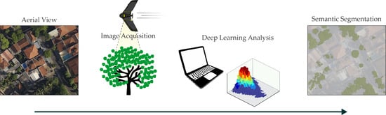
1. Introduction
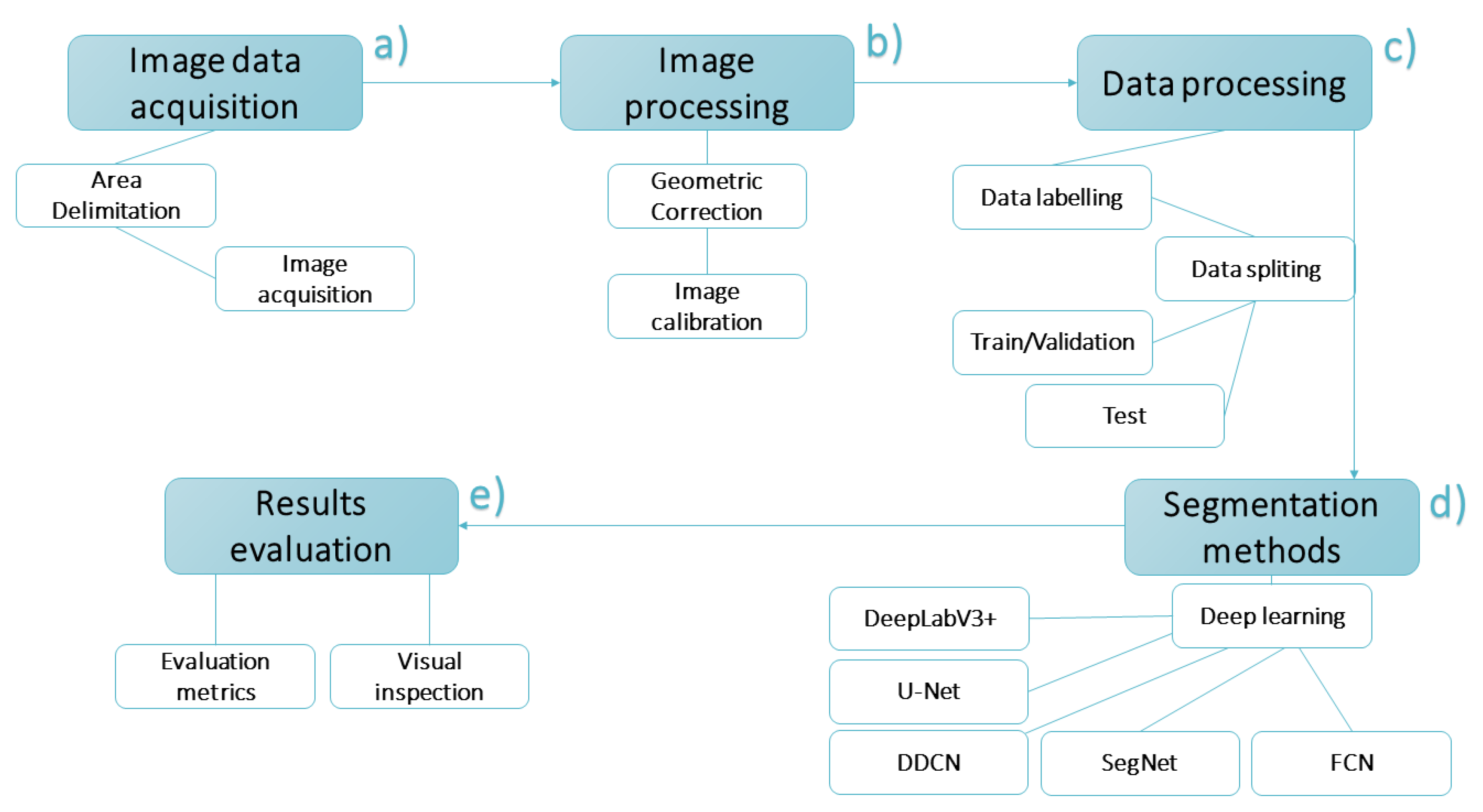
2. Materials and Methods
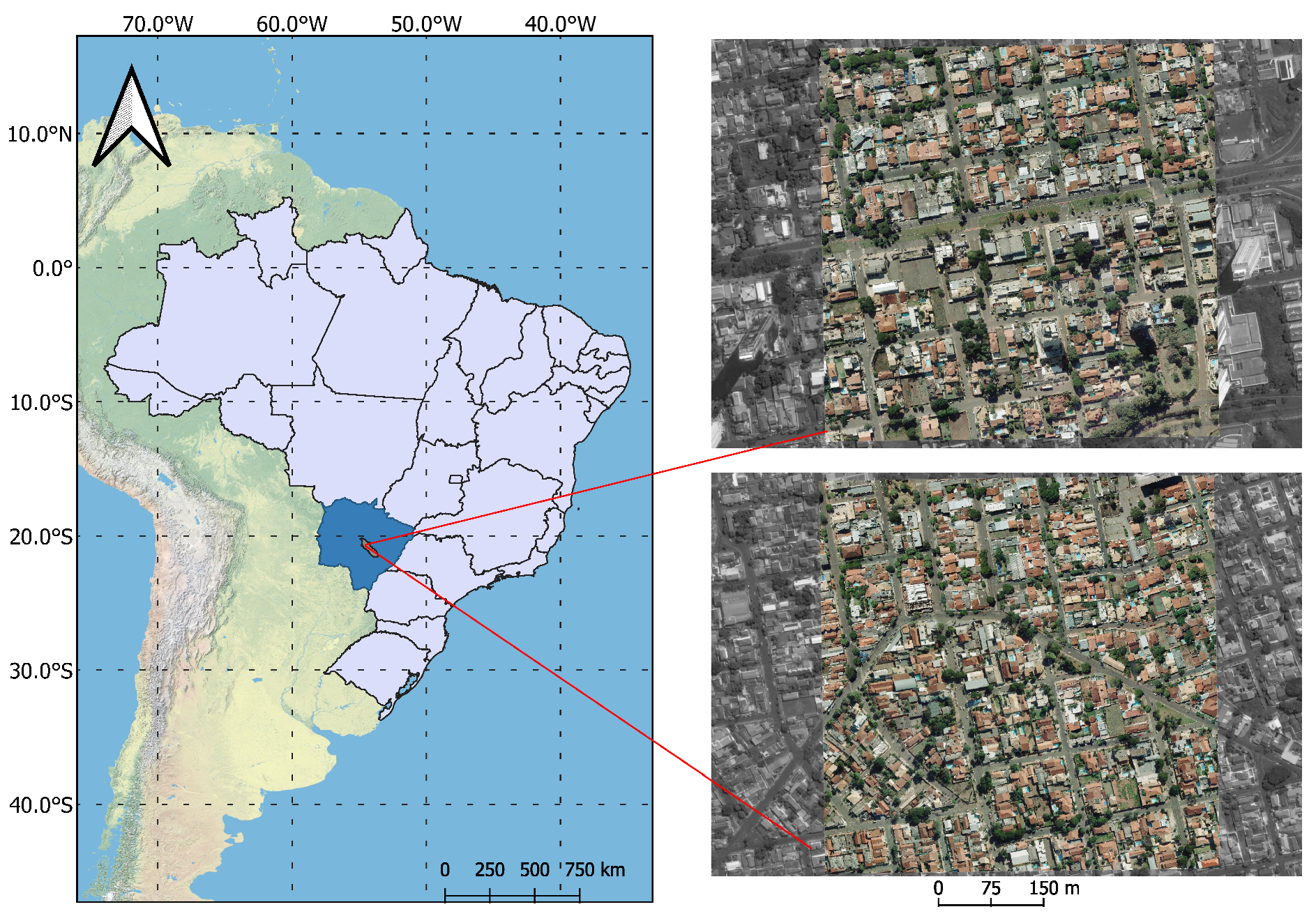
2.1. Data Acquisition and Image Processing
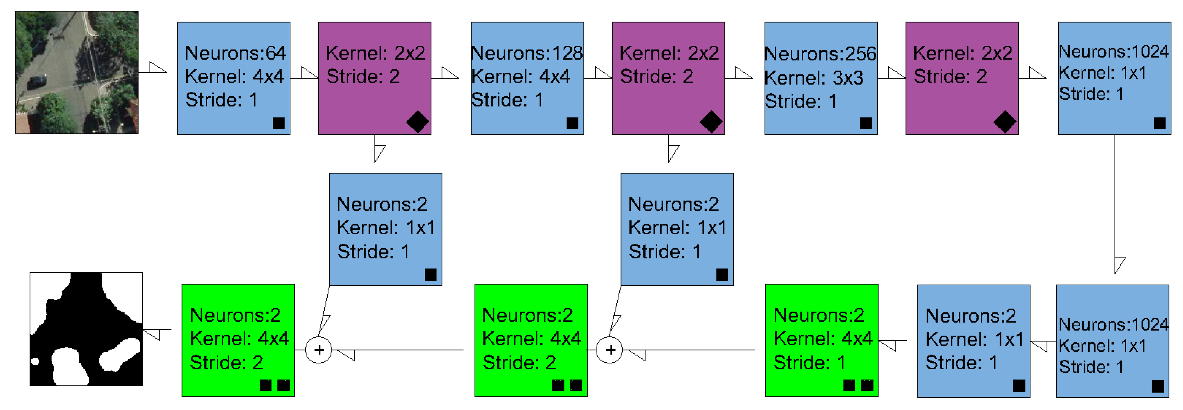
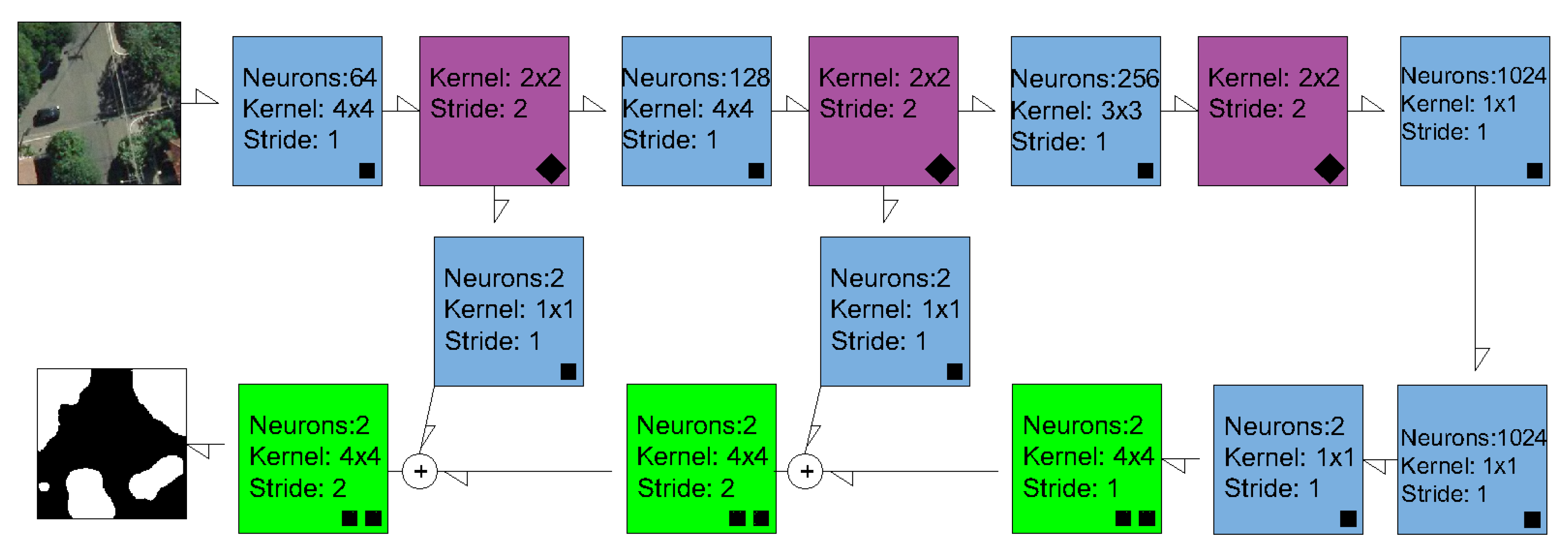
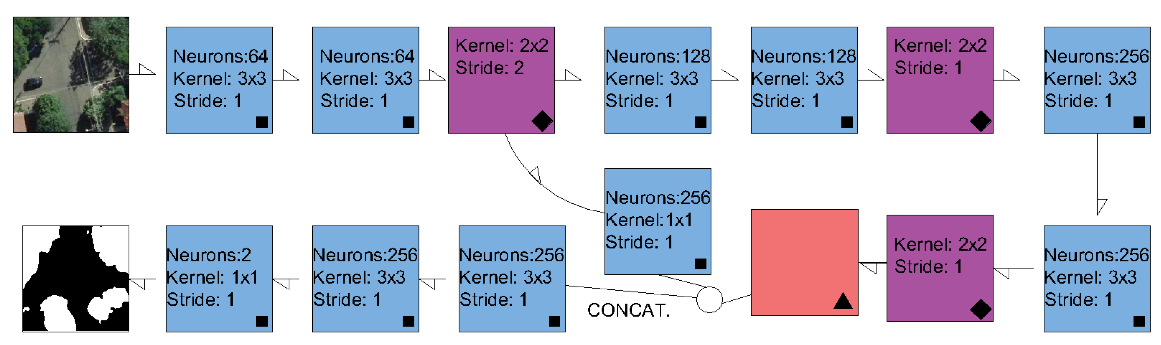
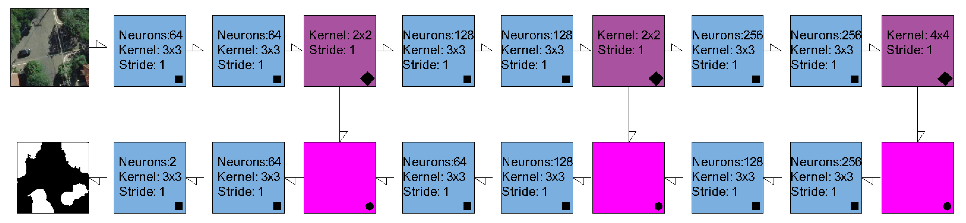
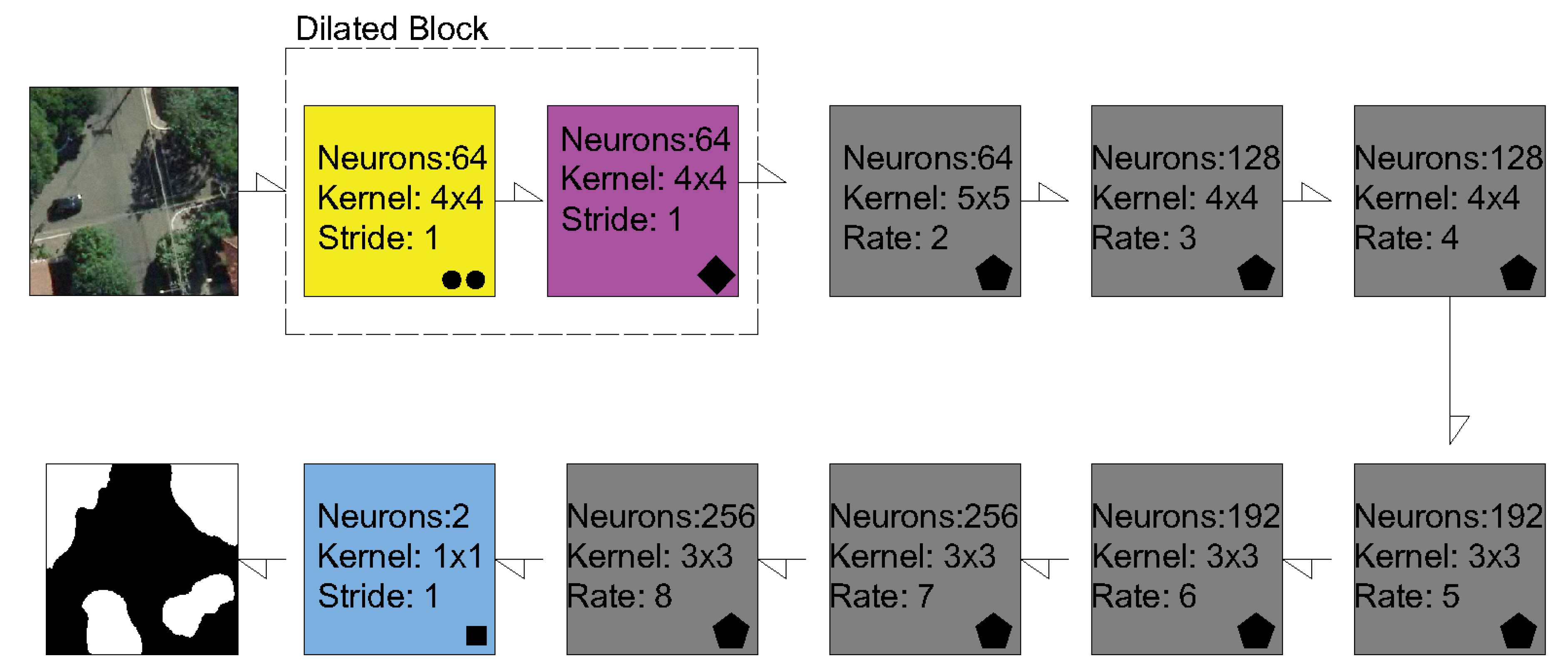
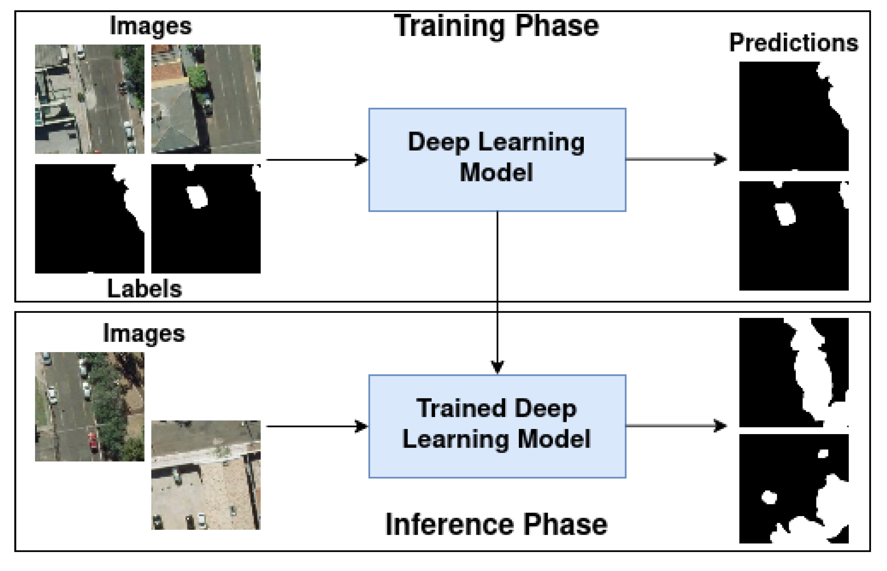
2.2. Semantic Segmentation Methods and Experimental Setup
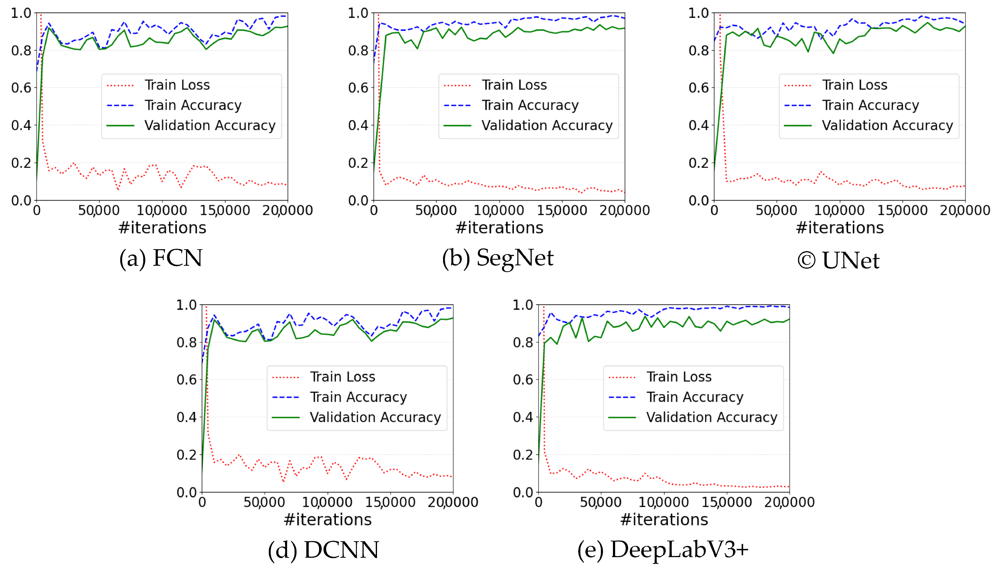
2.2.1. Experimental details
2.2.2. Evaluation Metrics
3. Results
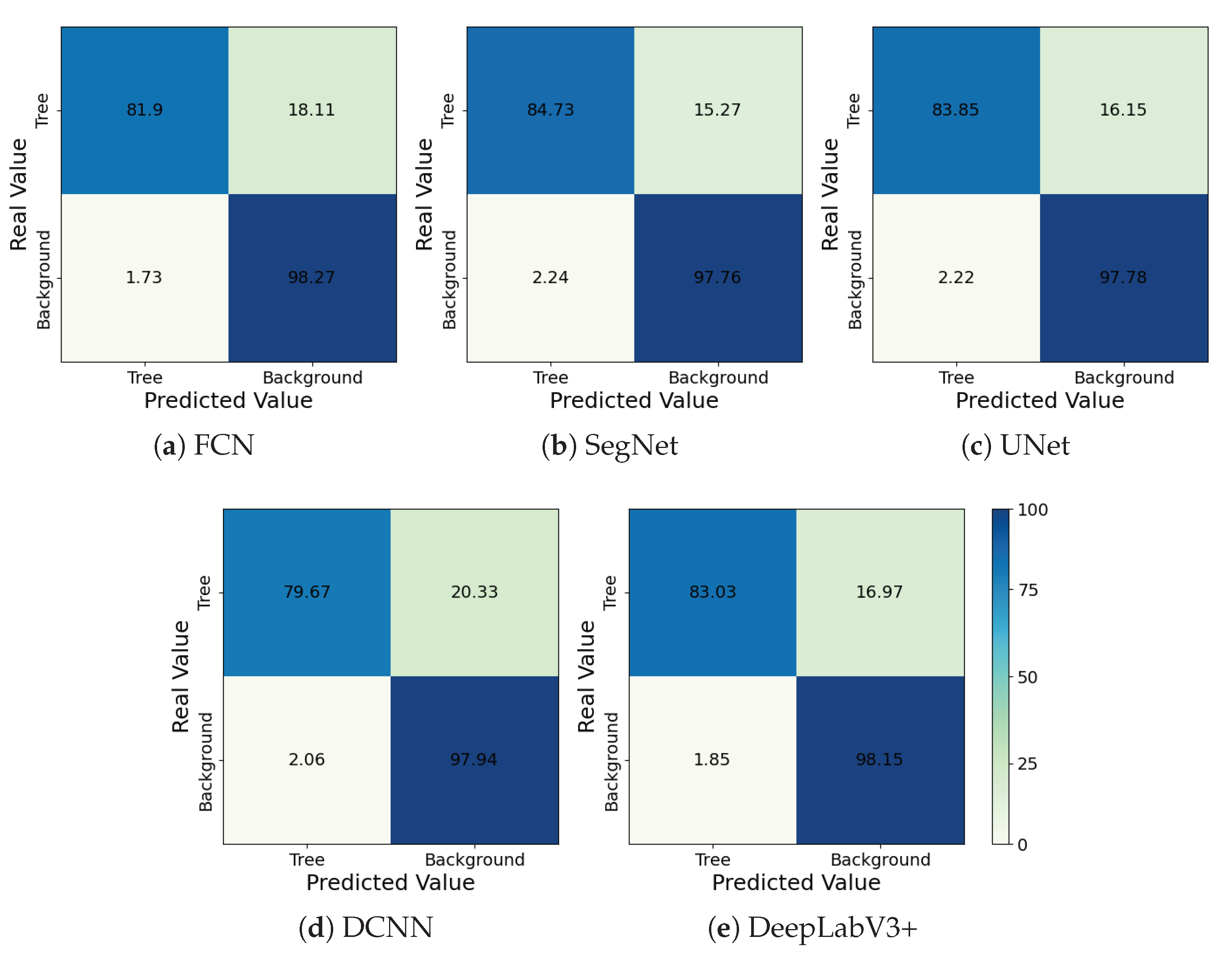
3.1. Performance Evaluation
3.2. Computational Complexity
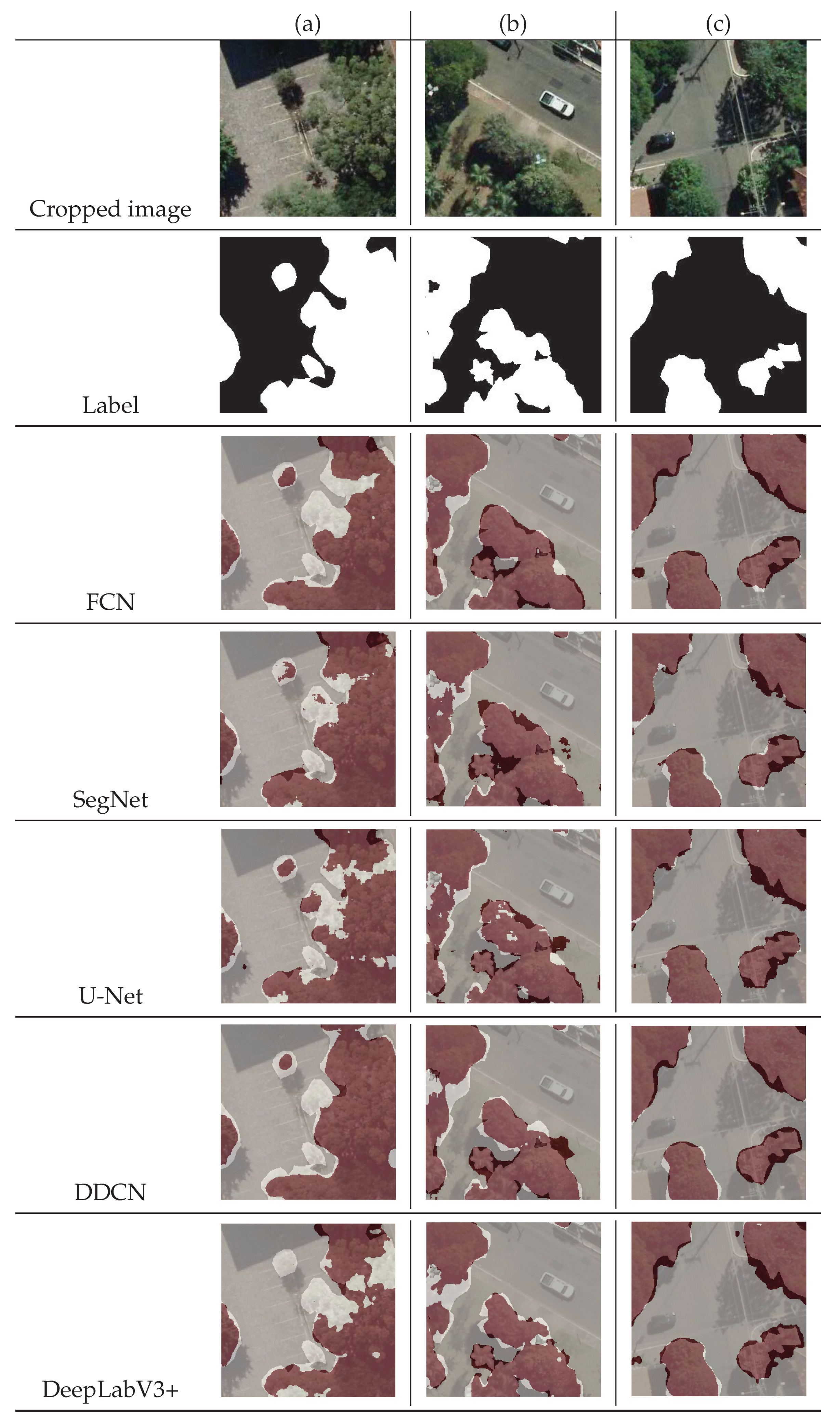
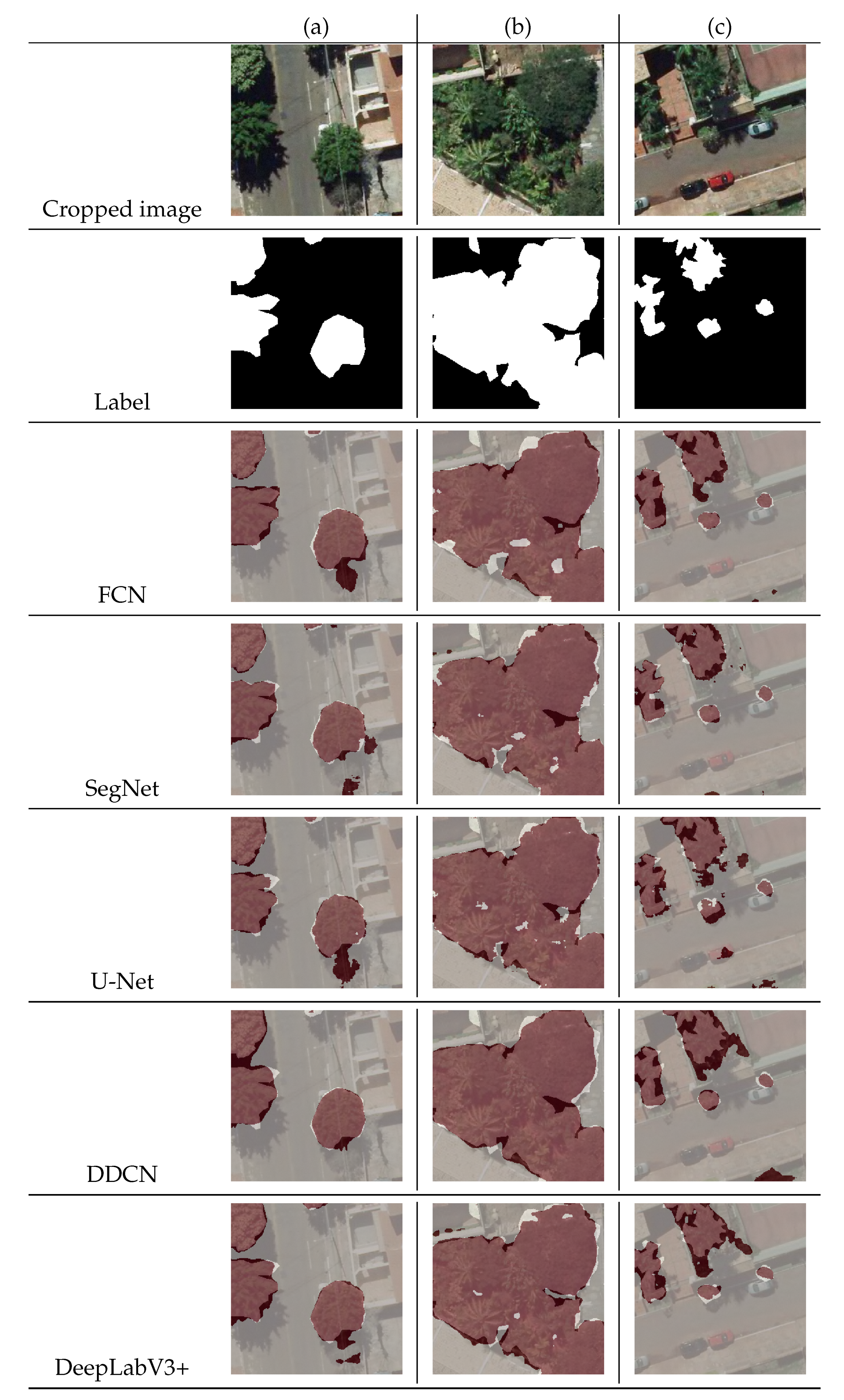
3.3. Visual Analysis
4. Discussion
5. Conclusions
Author Contributions
Funding
Data Availability Statement
Acknowledgments
Conflicts of Interest
References
- World Urbanization Prospects—Population Division—United Nations. 2018. Available online: https://population.un.org/wup/Publications/Files/WUP2018-Highlights.pdf (accessed on 16 July 2021).
- La Rosa, D.; Wiesmann, D. Land cover and impervious surface extraction using parametric and non-parametric algorithms from the open-source software R: An application to sustainable urban planning in Sicily. GIScience Remote Sens. 2013. [Google Scholar] [CrossRef]
- Jennings, V.L.L.; Yun, J. Advancing Sustainability through Urban Green Space: Cultural Ecosystem Services, Equity, and Social Determinants of Health. Int. J. Environ. Res. Public Health 2016, 13, 196. [Google Scholar] [CrossRef] [PubMed] [Green Version]
- Arantes, B.L.; Castro, N.R.; Gilio, L.; Polizel, J.L.; da Silva Filho, D.F. Urban forest and per capita income in the mega-city of Sao Paulo, Brazil: A spatial pattern analysis. Cities 2021, 111, 103099. [Google Scholar] [CrossRef]
- Jim, C.; Chen, W.Y. Ecosystem services and valuation of urban forests in China. Cities 2009, 26, 187–194. [Google Scholar] [CrossRef]
- Chen, W.Y.; Wang, D.T. Urban forest development in China: Natural endowment or socioeconomic product. Cities 2013, 35, 62–68. [Google Scholar] [CrossRef]
- Baró, F.; Chaparro, L.; Gómez-Baggethun, E.; Langemeyer, J.; Nowak, D.J.; Terradas, J. Contribution of ecosystem services to air quality and climate change mitigation policies: The case of urban forests in Barcelona, Spain. Ambio 2014. [Google Scholar] [CrossRef] [Green Version]
- McHugh, N.; Edmondson, J.L.; Gaston, K.J.; Leake, J.R.; O’Sullivan, O.S. Modelling short-rotation coppice and tree planting for urban carbon management—A citywide analysis. J. Appl. Ecol. 2015. [Google Scholar] [CrossRef]
- Kardan, O.; Gozdyra, P.; Misic, B.; Moola, F.; Palmer, L.J.; Paus, T.; Berman, M.G. Neighborhood greenspace and health in a large urban center. Sci. Rep. 2015. [Google Scholar] [CrossRef] [PubMed] [Green Version]
- Feng, Q.; Liu, J.; Gong, J. UAV Remote sensing for urban vegetation mapping using random forest and texture analysis. Remote Sens. 2015, 7, 1074–1094. [Google Scholar] [CrossRef] [Green Version]
- Alonzo, M.; McFadden, J.P.; Nowak, D.J.; Roberts, D.A. Mapping urban forest structure and function using hyperspectral imagery and lidar data. Urban For. Urban Green. 2016, 17, 135–147. [Google Scholar] [CrossRef] [Green Version]
- Liisa, T.; Stephan, P.; Klaus, S.; de Vries, S. Benefits and Uses of Urban Forests and Trees; Springer: Berlin/Heidelberg, Germany, 2005; pp. 81–114. [Google Scholar] [CrossRef]
- Song, X.P.; Hansen, M.; Stehman, S.; Potapov, P.; Tyukavina, A.; Vermote, E.; Townshend, J. Global land change from 1982 to 2016. Nature 2018, 639–643. [Google Scholar] [CrossRef] [PubMed]
- McGrane, S.J. GImpacts of urbanisation on hydrological and water quality dynamics, and urban water management: A review. Hydrol. Sci. J. 2015, 61, 2295–2311. [Google Scholar] [CrossRef]
- Schneider, A.; Friedl, M.A.; Potere, D. Mapping global urban areas using MODIS 500-m data: New methods and datasets based on ‘urban ecoregions’. Remote Sens. Environ. 2010, 114, 1733–1746. [Google Scholar] [CrossRef]
- Fassnacht, F.; Latifi, H.; Stereńczak, K.; Modzelewska, A.; Lefsky, M.; Waser, L.T.; Straub, C.; Ghosh, A. Review of studies on tree species classification from remotely sensed data. Remote Sens. Environ. 2016, 186, 64–87. [Google Scholar] [CrossRef]
- Onishi, M.; Ise, T. Automatic classification of trees using a UAV onboard camera and deep learning. arXiv 2018, arXiv:1804.10390. [Google Scholar]
- Jensen, R.R.; Hardin, P.J.; Bekker, M.; Farnes, D.S.; Lulla, V.; Hardin, A. Modeling urban leaf area index with AISA+ hyperspectral data. Appl. Geogr. 2009, 29, 320–332. [Google Scholar] [CrossRef]
- Lausch, A.; Erasmi, S.; King, D.J.; Magdon, P.; Heurich, M. Understanding forest health with Remote sensing-Part II-A review of approaches and data models. Remote Sens. 2017, 9, 129. [Google Scholar] [CrossRef] [Green Version]
- Colomina, I.; Molina, P. Unmanned aerial systems for photogrammetry and remote sensing: A review. ISPRS J. Photogramm. Remote Sens. 2014. [Google Scholar] [CrossRef] [Green Version]
- White, J.C.; Coops, N.C.; Wulder, M.A.; Vastaranta, M.; Hilker, T.; Tompalski, P. Remote Sensing Technologies for Enhancing Forest Inventories: A Review. Can. J. Remote Sens. 2016, 42, 619–641. [Google Scholar] [CrossRef] [Green Version]
- Adão, T.; Hruška, J.; Pádua, L.; Bessa, J.; Peres, E.; Morais, R.; Sousa, J.J. Hyperspectral imaging: A review on UAV-based sensors, data processing and applications for agriculture and forestry. Remote Sens. 2017, 9, 1110. [Google Scholar] [CrossRef] [Green Version]
- Arfaoui, A. Unmanned Aerial Vehicle: Review of Onboard Sensors, Application Fields, Open Problems and Research Issues; Technical Report; 2017; Available online: https://www.researchgate.net/publication/315076314_Unmanned_Aerial_Vehicle_Review_of_Onboard_Sensors_Application_Fields_Open_Problems_and_Research_Issues (accessed on 16 July 2021).
- Shojanoori, R.; Shafri, H.Z. Review on the use of remote sensing for urban forest monitoring. Arboric. Urban For. 2016, 42, 400–417. [Google Scholar]
- Alonzo, M.; Bookhagen, B.; Roberts, D. Urban tree species mapping using hyperspectral and LiDAR data fusion. Remote Sens. Environ. 2014, 148, 70–83. [Google Scholar] [CrossRef]
- Osco, L.P.; Ramos, A.P.M.; Pereira, D.R.; Moriya, É.A.S.; Imai, N.N.; Matsubara, E.T.; Estrabis, N.; de Souza, M.; Junior, J.M.; Gonçalves, W.N.; et al. Predicting canopy nitrogen content in citrus-trees using random forest algorithm associated to spectral vegetation indices from UAV-imagery. Remote Sens. 2019, 11, 2925. [Google Scholar] [CrossRef] [Green Version]
- Osco, L.P.; de Arruda, M.S.; Marcato Junior, J.; da Silva, N.B.; Ramos, A.P.M.; Moryia, É.A.S.; Imai, N.N.; Pereira, D.R.; Creste, J.E.; Matsubara, E.T.; et al. A convolutional neural network approach for counting and geolocating citrus-trees in UAV multispectral imagery. ISPRS J. Photogramm. Remote Sens. 2020. [Google Scholar] [CrossRef]
- Martins, J.; Junior, J.M.; Menezes, G.; Pistori, H.; Sant’Ana, D.; Goncalves, W. Image Segmentation and Classification with SLIC Superpixel and Convolutional Neural Network in Forest Context. In Proceedings of the IGARSS 2019—2019 IEEE International Geoscience and Remote Sensing Symposium, Yokohama, Japan, 28 July–2 August 2019; pp. 6543–6546. [Google Scholar] [CrossRef]
- dos Santos Ferreira, A.; Matte Freitas, D.; Gonçalves da Silva, G.; Pistori, H.; Theophilo Folhes, M. Weed detection in soybean crops using ConvNets. Comput. Electron. Agric. 2017, 143, 314–324. [Google Scholar] [CrossRef]
- Torres, D.L.; Feitosa, R.Q.; Happ, P.N.; La Rosa, L.E.C.; Junior, J.M.; Martins, J.; Bressan, P.O.; Gonçalves, W.N.; Liesenberg, V. Applying fully convolutional architectures for semantic segmentation of a single tree species in urban environment on high resolution UAV optical imagery. Sensors 2020, 20, 563. [Google Scholar] [CrossRef] [Green Version]
- Zhang, Q.; Xu, J.; Xu, L.; Guo, H. Deep Convolutional Neural Networks for Forest Fire Detection. In Proceedings of the 2016 International Forum on Management, Education and Information Technology Application, Guangzhou, China, 30–31 January 2016; pp. 568–575. [Google Scholar] [CrossRef] [Green Version]
- Bazi, Y.; Melgani, F. Convolutional SVM Networks for Object Detection in UAV Imagery. IEEE Trans. Geosci. Remote Sens. 2018, 56, 3107–3118. [Google Scholar] [CrossRef]
- Zhao, X.; Yuan, Y.; Song, M.; Ding, Y.; Lin, F.; Liang, D. Use of Unmanned Aerial Vehicle Imagery and Deep Learning UNet to Extract Rice Lodging. Sensors 2019, 19, 3859. [Google Scholar] [CrossRef] [Green Version]
- Ganesh, P.; Volle, K.; Burks, T.F.; Mehta, S.S. Deep Orange: Mask R-CNN based Orange Detection and Segmentation. IFAC-PapersOnLine 2019. [Google Scholar] [CrossRef]
- Nogueira, K.; Dalla Mura, M.; Chanussot, J.; Schwartz, W.R.; Dos Santos, J.A. Dynamic multicontext segmentation of remote sensing images based on convolutional networks. IEEE Trans. Geosci. Remote Sens. 2019. [Google Scholar] [CrossRef] [Green Version]
- Zamboni, P.; Junior, J.M.; Silva, J.d.A.; Miyoshi, G.T.; Matsubara, E.T.; Nogueira, K.; Gonçalves, W.N. Benchmarking Anchor-Based and Anchor-Free State-of-the-Art Deep Learning Methods for Individual Tree Detection in RGB High-Resolution Images. Remote Sens. 2021, 13, 2482. [Google Scholar] [CrossRef]
- Pestana, L.; Alves, F.; Sartori, Â. Espécies arbóreas da arborização urbana do centro do município de campo grande, mato grosso do sul, brasil. Rev. Soc. Bras. Arborização Urbana 2019, 6, 1–21. [Google Scholar] [CrossRef]
- Ososkov, G.; Goncharov, P. Shallow and deep learning for image classification. Opt. Mem. Neural Netw. 2017, 26, 221–248. [Google Scholar] [CrossRef]
- Walsh, J.; O’ Mahony, N.; Campbell, S.; Carvalho, A.; Krpalkova, L.; Velasco-Hernandez, G.; Harapanahalli, S.; Riordan, D. Deep Learning vs. Traditional Computer Vision. Tradit. Comput. Vis. 2019. [Google Scholar] [CrossRef] [Green Version]
- Liu, X.; Faes, L.; Kale, A.U.; Wagner, S.K.; Fu, D.J.; Bruynseels, A.; Mahendiran, T.; Moraes, G.; Shamdas, M.; Kern, C.; et al. A comparison of deep learning performance against health-care professionals in detecting diseases from medical imaging: A systematic review and meta-analysis. Lancet Digit. Health 2019, 1, e271–e297. [Google Scholar] [CrossRef]
- Bui, D.T.; Tsangaratos, P.; Nguyen, V.T.; Liem, N.V.; Trinh, P.T. Comparing the prediction performance of a Deep Learning Neural Network model with conventional machine learning models in landslide susceptibility assessment. CATENA 2020, 188, 104426. [Google Scholar] [CrossRef]
- Sujatha, R.; Chatterjee, J.M.; Jhanjhi, N.; Brohi, S.N. Performance of deep learning vs machine learning in plant leaf disease detection. Microprocess. Microsyst. 2021, 80, 103615. [Google Scholar] [CrossRef]
- Osco, L.P.; Nogueira, K.; Ramos, A.P.M.; Pinheiro, M.M.F.; Furuya, D.E.G.; Gonçalves, W.N.; de Castro Jorge, L.A.; Junior, J.M.; dos Santos, J.A. Semantic segmentation of citrus-orchard using deep neural networks and multispectral UAV-based imagery. Precis. Agric. 2021. [Google Scholar] [CrossRef]
- Long, J.; Shelhamer, E.; Darrell, T. Fully Convolutional Networks for Semantic Segmentation. In Proceedings of the IEEE Conference on Computer Vision and Pattern Recognition, Boston, MA, USA, 7–12 June 2015. [Google Scholar] [CrossRef] [Green Version]
- Ronneberger, O.; Fischer, P.; Brox, T. U-Net: Convolutional Networks for Biomedical. In Proceedings of the International Conference on Medical Image Computing and Computer-Assisted Intervention, Munich, Germany, 5–9 October 2015. [Google Scholar] [CrossRef] [Green Version]
- Badrinarayanan, V.; Kendall, A.; Cipolla, R. SegNet: A Deep Convolutional Encoder-Decoder Architecture for Image Segmentation. IEEE Trans. Pattern Anal. Mach. Intell. 2017, 39, 2481–2495. [Google Scholar] [CrossRef]
- Simonyan, K.; Zisserman, A. Very Deep Convolutional Networks for Large-Scale Image Recognition. arXiv 2014, arXiv:1409.1556. [Google Scholar]
- Chen, L.C.; Papandreou, G.; Kokkinos, I.; Murphy, K.; Yuille, A.L. DeepLab: Semantic Image Segmentation with Deep Convolutional Nets, Atrous Convolution, and Fully Connected CRFs. IEEE Trans. Pattern Anal. Mach. Intell. 2018. [Google Scholar] [CrossRef] [PubMed]
- Chen, S.W.; Shivakumar, S.S.; Dcunha, S.; Das, J.; Okon, E.; Qu, C.; Taylor, C.J.; Kumar, V. Counting Apples and Oranges with Deep Learning: A Data-Driven Approach. IEEE Robot. Autom. Lett. 2017. [Google Scholar] [CrossRef]
- Volpi, M.; Tuia, D. Dense Semantic Labeling of Subdecimeter Resolution Images with Convolutional Neural Networks. IEEE Trans. Geosci. Remote Sens. 2017, 55, 881–893. [Google Scholar] [CrossRef] [Green Version]
- Abadi, M.; Agarwal, A.; Barham, P.; Brevdo, E.; Chen, Z.; Citro, C.; Corrado, G.S.; Davis, A.; Dean, J.; Devin, M.; et al. TensorFlow: Large-Scale Machine Learning on Heterogeneous Systems. 2015. Available online: tensorflow.org (accessed on 16 July 2021).
- Cohen, J. A Coefficient of Agreement for Nominal Scales. Educ. Psychol. Meas. 1960, 20, 37–46. [Google Scholar] [CrossRef]
- Wu, Z.; Gao, Y.; Li, L.; Xue, J.; Li, Y. Semantic segmentation of high-resolution remote sensing images using fully convolutional network with adaptive threshold. Connect. Sci. 2019. [Google Scholar] [CrossRef]
- Berman, M.; Triki, A.R.; Blaschko, M.B. The Lovasz-Softmax Loss: A Tractable Surrogate for the Optimization of the Intersection-Over-Union Measure in Neural Networks. In Proceedings of the IEEE Computer Society Conference on Computer Vision and Pattern Recognition, Salt Lake City, UT, USA, 18–23 June 2018. [Google Scholar] [CrossRef] [Green Version]
- LeCun, Y.; Bengio, Y.; Hinton, G. Deep Learning. Nature 2015, 521, 436–444. [Google Scholar] [CrossRef] [PubMed]
- Goodfellow, I.; Bengio, Y.; Courville, A. Deep Learning; MIT Press: Cambridge, MA, USA, 2016; Available online: http://www.deeplearningbook.org (accessed on 16 July 2021).
- Madawy, K.E.; Rashed, H.; Sallab, A.E.; Nasr, O.; Kamel, H.; Yogamani, S. Rgb and lidar fusion based 3d semantic segmentation for autonomous driving. arXiv 2019, arXiv:1906.00208. [Google Scholar]
- Zhao, X.; Sun, P.; Xu, Z.; Min, H.; Yu, H. Fusion of 3D LIDAR and Camera Data for Object Detection in Autonomous Vehicle Applications. IEEE Sens. J. 2020, 20, 4901–4913. [Google Scholar] [CrossRef] [Green Version]
- Zheng, G.; Moskal, L.M. Retrieving Leaf Area Index (LAI) Using Remote Sensing: Theories, Methods and Sensors. Sensors 2009, 9, 2719–2745. [Google Scholar] [CrossRef] [PubMed] [Green Version]


| Set | Network | Pix. Acc. | Av. Acc. | F1-Score | Kappa | IoU |
|---|---|---|---|---|---|---|
| Test. | FCN | 0.9614 | 0.9008 | 0.9123 | 0.8247 | 0.7342 |
| SegNet | 0.9607 | 0.9125 | 0.9130 | 0.8260 | 0.7370 | |
| U-Net | 0.9597 | 0.9082 | 0.9104 | 0.8208 | 0.7301 | |
| DDCN | 0.9556 | 0.8880 | 0.8991 | 0.7983 | 0.7001 | |
| DeepLabV3+ | 0.9618 | 0.9059 | 0.9140 | 0.8280 | 0.7389 |
| Method | FCN | U-Net | SegNet | DeepLabV3+ | DDCN |
|---|---|---|---|---|---|
| Number of Parameters (in millions) | 3.83 | 1.86 | 2.32 | 5.16 | 2.08 |
| Training Time (GPU hours) | 485 | 450 | 472 | 486 | 500 |
| Inference Time (GPU min.) | 1.4 | 1 | 1.1 | 1.4 | 5.1 |
| Inference Time (CPU min.) | 1.9 | 1.3 | 1.5 | 1.9 | 6.2 |
| Inference Time (GPU min./ha) | 0.042 | 0.030 | 0.033 | 0.042 | 0.153 |
| Inference Time (CPU min./ha) | 0.057 | 0.039 | 0.045 | 0.057 | 0.186 |
Publisher’s Note: MDPI stays neutral with regard to jurisdictional claims in published maps and institutional affiliations. |
© 2021 by the authors. Licensee MDPI, Basel, Switzerland. This article is an open access article distributed under the terms and conditions of the Creative Commons Attribution (CC BY) license (https://creativecommons.org/licenses/by/4.0/).
Share and Cite
Martins, J.A.C.; Nogueira, K.; Osco, L.P.; Gomes, F.D.G.; Furuya, D.E.G.; Gonçalves, W.N.; Sant’Ana, D.A.; Ramos, A.P.M.; Liesenberg, V.; dos Santos, J.A.; et al. Semantic Segmentation of Tree-Canopy in Urban Environment with Pixel-Wise Deep Learning. Remote Sens. 2021, 13, 3054. https://0-doi-org.brum.beds.ac.uk/10.3390/rs13163054
Martins JAC, Nogueira K, Osco LP, Gomes FDG, Furuya DEG, Gonçalves WN, Sant’Ana DA, Ramos APM, Liesenberg V, dos Santos JA, et al. Semantic Segmentation of Tree-Canopy in Urban Environment with Pixel-Wise Deep Learning. Remote Sensing. 2021; 13(16):3054. https://0-doi-org.brum.beds.ac.uk/10.3390/rs13163054
Chicago/Turabian StyleMartins, José Augusto Correa, Keiller Nogueira, Lucas Prado Osco, Felipe David Georges Gomes, Danielle Elis Garcia Furuya, Wesley Nunes Gonçalves, Diego André Sant’Ana, Ana Paula Marques Ramos, Veraldo Liesenberg, Jefersson Alex dos Santos, and et al. 2021. "Semantic Segmentation of Tree-Canopy in Urban Environment with Pixel-Wise Deep Learning" Remote Sensing 13, no. 16: 3054. https://0-doi-org.brum.beds.ac.uk/10.3390/rs13163054