Technical Note

A New Method for Automated Measurement of Sand Dune Migration Based on Multi-Temporal LiDAR-Derived Digital Elevation Models

1
Department of Geography and the Environment, University of North Texas, Denton, TX 76203, USA
2
School of Earth Sciences, Yunnan University, Kunming 650500, China
3
Beijing Advanced Innovation Center for Imaging Theory and Technology, Capital Normal University, 105 West Third Ring North Road, Haidian District, Beijing 100048, China
4
MNR Key Laboratory of Sanjiang Metallogeny and Resource Exploration & Utilization, Kunming 650500, China
*
Author to whom correspondence should be addressed.
Remote Sens. 2021, 13(16), 3084; https://0-doi-org.brum.beds.ac.uk/10.3390/rs13163084
Submission received: 30 June 2021 / Revised: 30 July 2021 / Accepted: 3 August 2021 / Published: 6 August 2021
(This article belongs to the Special Issue Advances of Remote Sensing in Environmental Geoscience)

Abstract

:
While remote sensing methods have long been used for coastal and desert sand dune studies, few methods have been developed for the automated measurement of dune migration in large dune fields. To overcome a major limitation of an existing method named “pairs of source and target points (PSTP)”, this paper proposes a toe line tracking (TLT) method for the automated measurement of dune migration rate and direction using multi-temporal digital elevation models (DEM) derived from light detection and ranging (LiDAR) data. Based on a few simple parameters, the TLT method automatically extracts the base level of a dune field and toe lines of individual dunes. The toe line polygons derived from two DEMs are processed using logical operators and other spatial analysis methods implemented in the Python programming language in a geographic information system. By generating thousands of random sampling points along source toe lines, dune migration distances and directions are calculated and saved with the sampling point feature class. The application of the TLT method was demonstrated using multi-temporal LiDAR-derived DEMs for a 9 km by 2.4 km area in the White Sands Dune Field in New Mexico (USA). Dune migration distances and directions for three periods (24 January 2009–26 September 2009, 26 September 2009–6 June 2010, and 24 January 2009–6 January 2010) were calculated. Sensitivity analyses were carried out using different window sizes and toe heights. The results suggest that both PSTP and TLT produce similar sand dune migration rates and directions, but TLT is a more generic method that works for dunes with or without slipfaces that reach the angle of repose.

Graphical Abstract

1. Introduction

Understanding how sand dunes form and change on Earth and some other planets (such as Mars, Venus, and Titan) has long been a research topic in Earth and planetary surface processes [1,2,3,4,5,6,7,8]. While studies in the 1970s and 1980s mainly focused on individual sand dunes, the advances in data collection and analysis enable studying dunes as complex systems [9], including numerous field studies around the world [10,11,12,13,14,15], quantitative/numerical models [16,17,18,19,20,21], and remote sensing methods [22,23,24,25,26,27,28,29,30,31,32,33,34,35]. These studies have led to a better understanding of sand dunes.
While remote sensing methods have been used for studies of coastal and desert sand dunes for decades, the objectivity of visual image interpretation and manual measurement methods has been questioned [36]. In addition, visual image interpretation and manual measurement can be very labor-intensive and time-consuming for large dune fields. In comparison with traditional medium- and low-resolution remote sensing methods, light detection and ranging (LiDAR) has provided unprecedented high-resolution and high-accuracy digital elevation models (DEM) for sand dune studies, from coastal dunes [37,38,39] to desert dunes [40,41,42,43,44]. However, it appears that traditional manual delineation and measurement of sand dune features is still a common practice, and that the unique capability of LiDAR in providing three-dimensional information on topographic details is not fully utilized. As reviewed by Hugenholtz et al. [45], the progress in spatial analysis methods for characterizing dune field patterns has been limited. A review of LiDAR data for change detection in Earth sciences can be found in Okyay et al. [46].
To facilitate the investigation of large dune fields using LiDAR data, Dong [44] developed a new approach, pairs of source and target points (PSTP), for the automated measurement of sand dune migration rates and directions in a geographic information system (GIS). Using LiDAR data collected for a 2.4 km by 9 km area in the White Sands Dune Field (WSDF) in New Mexico, USA on 24 January 2009 and 6 June 2010, Dong [44] demonstrated that sand dune migration rates and directions in large dune fields can be automatically detected and measured using multi-temporal LiDAR-derived DEMs at thousands of locations in minutes. A PSTP software tool was also developed by Xia and Dong [47] for the automated measurement of sand dune migration rates and directions.
A major limitation of the PSTP method developed by Dong [44] is that it requires obvious dune slipfaces that reach the angle of repose (30° to 34°) in both DEMs. This requirement can be difficult to meet if one or both DEMs are created from data collected when sand dune slipfaces do not reach the angle of repose due to seasonal winds. In fact, few slipfaces reached the angle of repose in the DEM derived from LiDAR collected in WSDF on 26 September 2009 due to the influence of reverse winds or crosswinds. Figure 1 shows three west–east profiles of a dune in WSDF extracted from LiDAR-derived DEMs of 24 January 2009; 26 September 2009; and 6 June 2010. As can be seen in Figure 1, the September 26, 2009 profile has a reversed crestline compared with the 24 January 2009 profile, and a leeward slope of about 28°, less than the angle of repose (about 34°) shown by the slipfaces in the other two profiles. It should be noted that the 26 September 2009 profile still shows a net migration of the dune following the prevailing wind direction. However, the PSTP method is unable to measure the migration from 24 January 2009 to 26 September 2009, or from 26 September 2009 to 6 June 2010 due to the lack of slipfaces that reach the angle of repose in the 26 September 2009 profile. The reversed crestline of 26 September 2009 also suggests that crestline positions are not reliable for measuring sand dune migration in this case.
To overcome the above major limitation of the PSTP method, this paper proposes a new method called toe line tracking (TLT) for the automated measurement of sand dune migration distance and direction using multi-temporal DEMs derived from LiDAR data in a study area in the White Sands Dune Field (WSDF) in New Mexico, USA. Compared with the PSTP method which relies on the angle of repose for sand dune, the new method aims to extract toe lines of sand dunes based on several simple parameters, and conduct automated measurement of dune migration rates and directions through random sampling and spatial analysis in geographic information systems (GIS). The study area, data, methods, results, discussion, and conclusions are presented in the following sections.

2. Study Area and Data
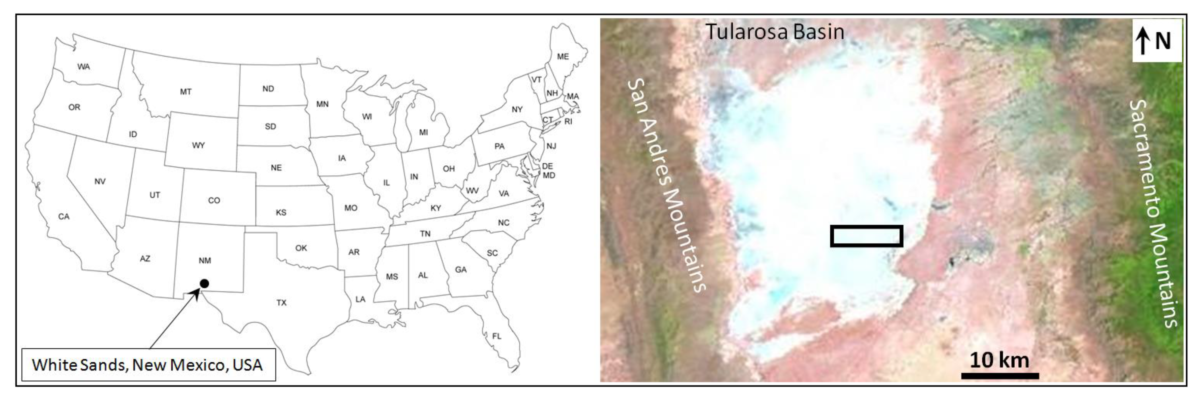
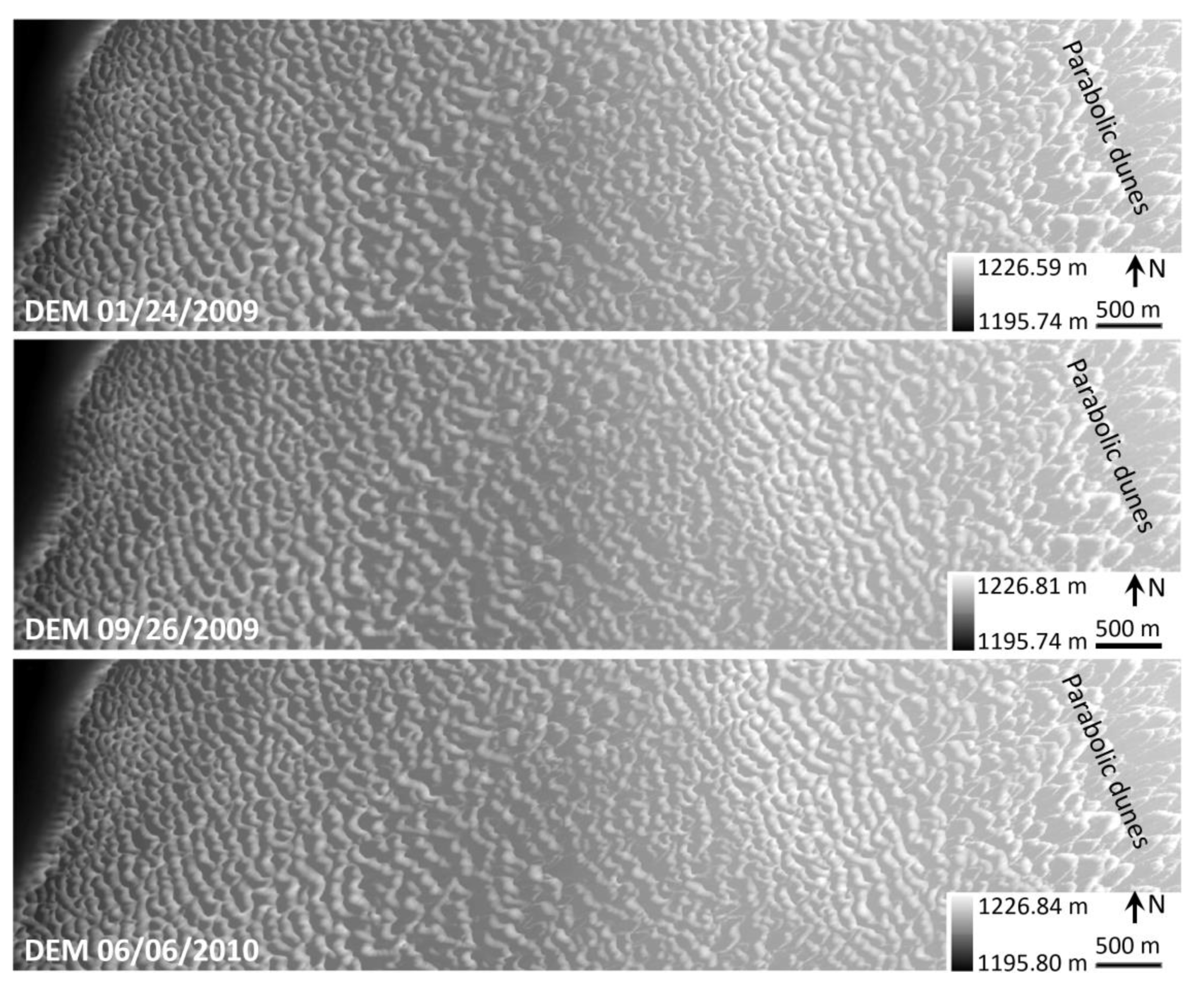
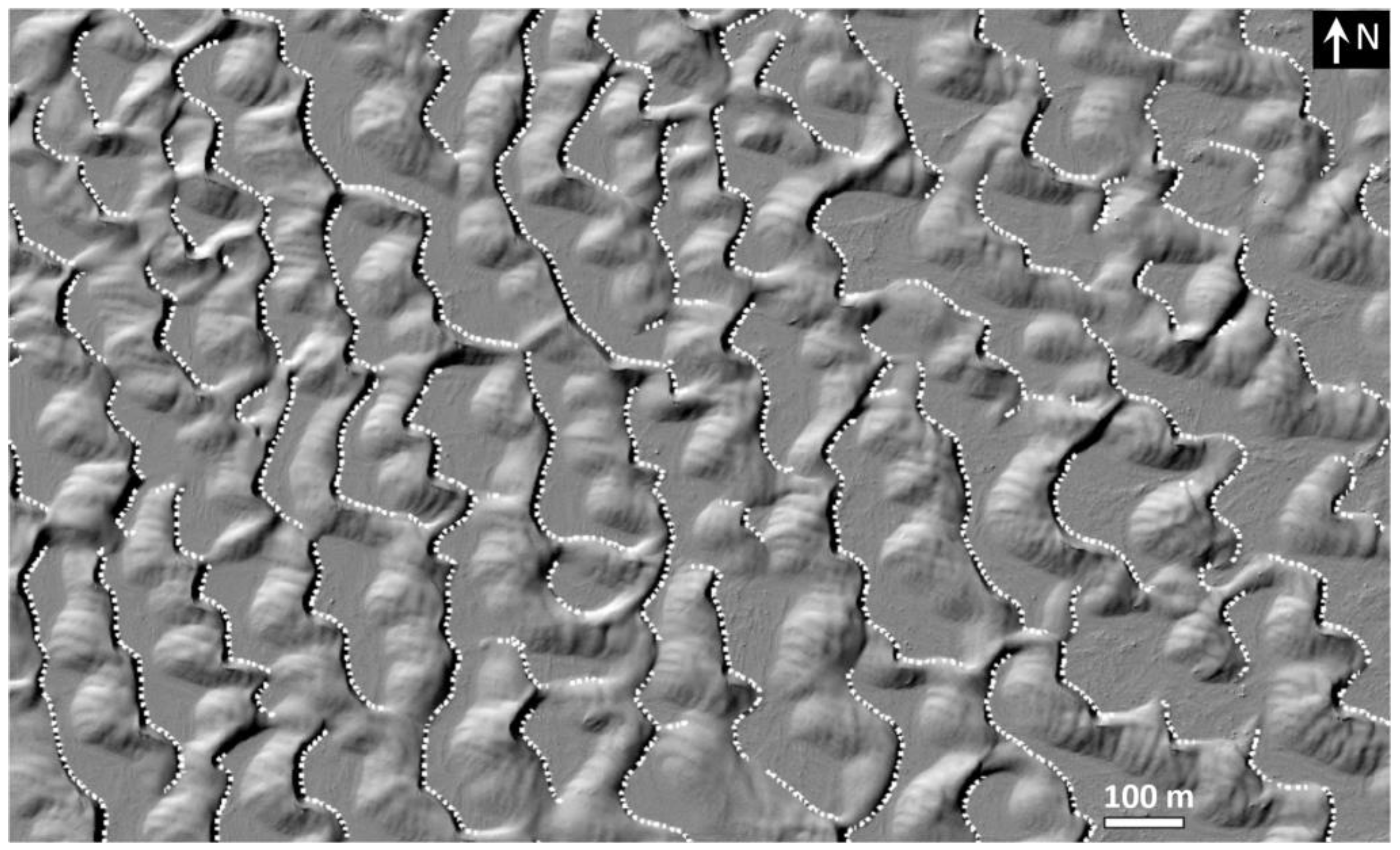
2.1. Study Area

A study area of 9 × 2.4 km in the White Sands Dune Field (WSDF) in New Mexico, USA is selected. WSDF is a gypsum dune field with an area of about 500 km2 in the Tularosa Basin between the San Andres Mountains and the Sacramento Mountains (Figure 2). The deflation of evaporite beds of Lake Otero and other playa lakes in the basin is the major sediment source of WSDF [48]. The selected study area has three types of dunes—barchans, transverse, and parabolic—with up to 15 m in height. The general trend of the crestlines is NNW (345°), and the average spacing of the crestlines is 136 m (Ewing et al. 2006). The dominant winds from the SW–W are strongest during the winter–spring, while winds from the N–NW occur during the fall-winter, and winds from the S–SE occur during the spring–summer [48]. WSDF has been well documented in numerous studies [41,42,48,49,50,51].

2.2. Data

LiDAR point clouds acquired on 24 January 2009; 26 September 2009; and 6 June 2010 in the study area were downloaded from the OpenTopography Facility (www.OpenTopography.org, accessed on 2 March 2015) at the San Diego Supercomputer Center. LiDAR data acquisition and processing was completed by the National Center for Airborne Laser Mapping (NCALM—http://www.ncalm.org (accessed date 2 August 2021)). The point densities of the three datasets are 4.19 points/m2, 5.63 points/m2, and 4.62 points/m2, respectively. The horizontal coordinate system is NAD83 UTM Zone 13N, and the vertical coordinate system is NAVD88. The vertical accuracy of the datasets are less than 0.35 m. Figure 3 shows the digital elevation models (DEM) created from the multi-temporal LiDAR point clouds using Inverse Distance Weighted (IDW) interpolation with a cell size of 1 × 1 m. The IDW interpolation method was selected because (1) the LiDAR point densities are high enough for a cell size of 1 × 1 m; and (2) the results in this paper will be compared with the results from Dong [44] which was based on IDW interpolation of LiDAR points.

3. Methods

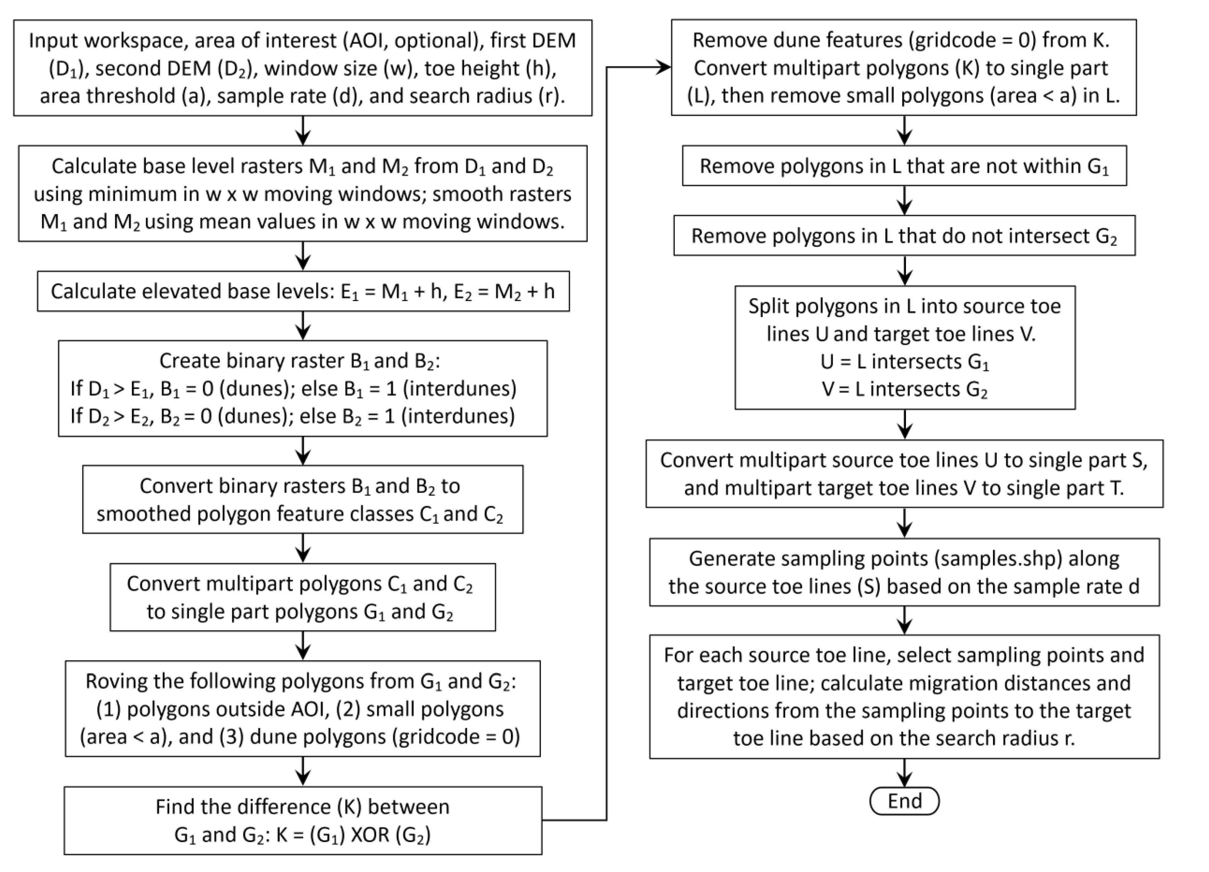
3.1. Methodology Flowchart

The methodology flowchart for toe line tracking (TLT) is shown in Figure 4. The process is implemented using the Python programming language and ArcPy for ArcGIS 10.7 with ArcGIS Desktop Advanced License. The user input parameters include workspace (folder for output files), area of interest (AOI, optional), first DEM (D1), second DEM (D2), window size (w), toe height (h), area threshold (a), sample rate (d), and search radius (r). With these initial parameters, the whole process in the flowchart is executed automatically. The flowchart can be implemented in other GIS packages. More details of the major steps in the flowchart are explained in the following sections.

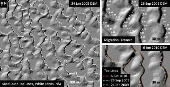
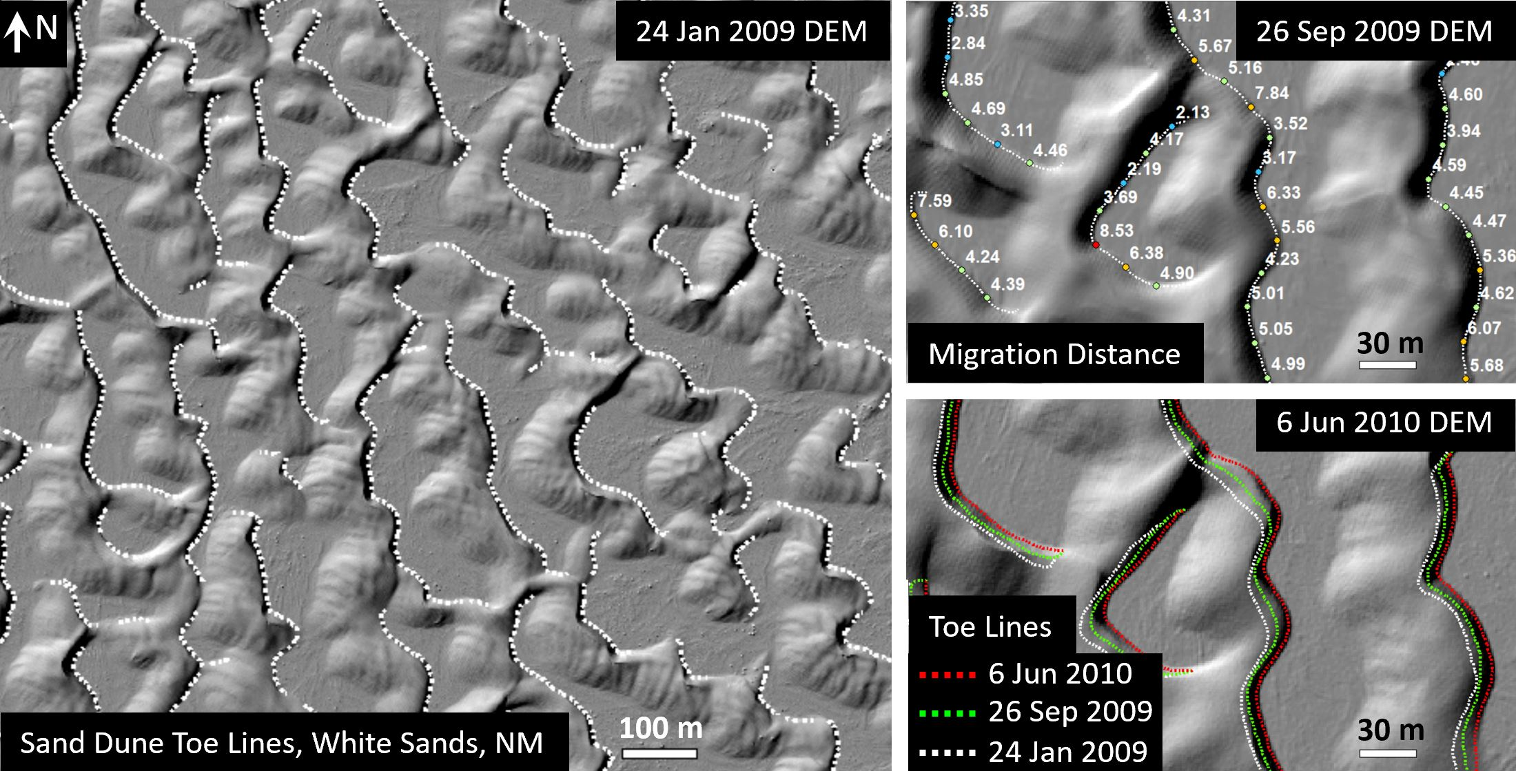
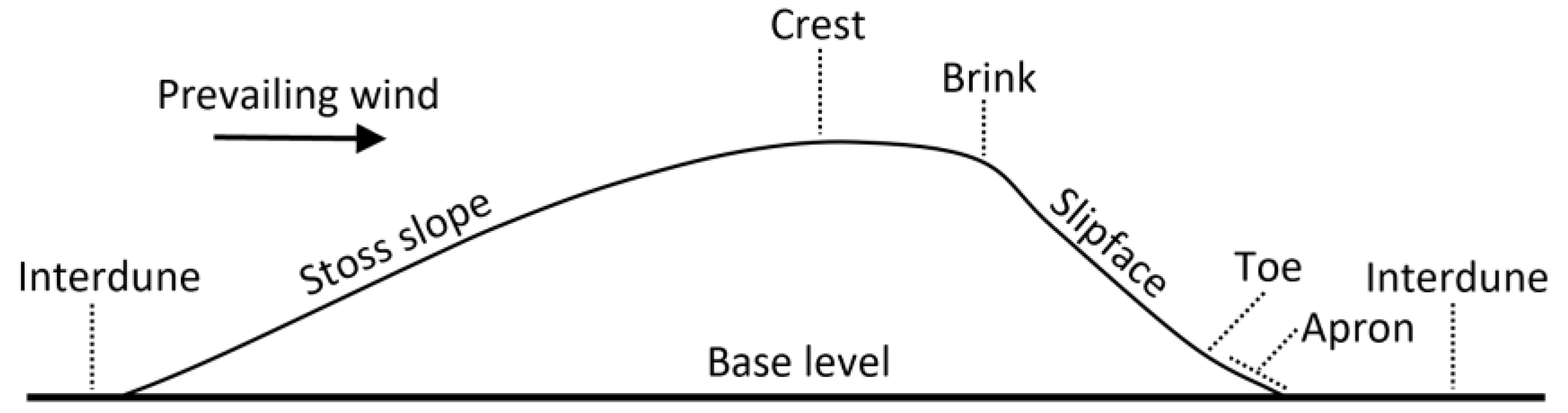
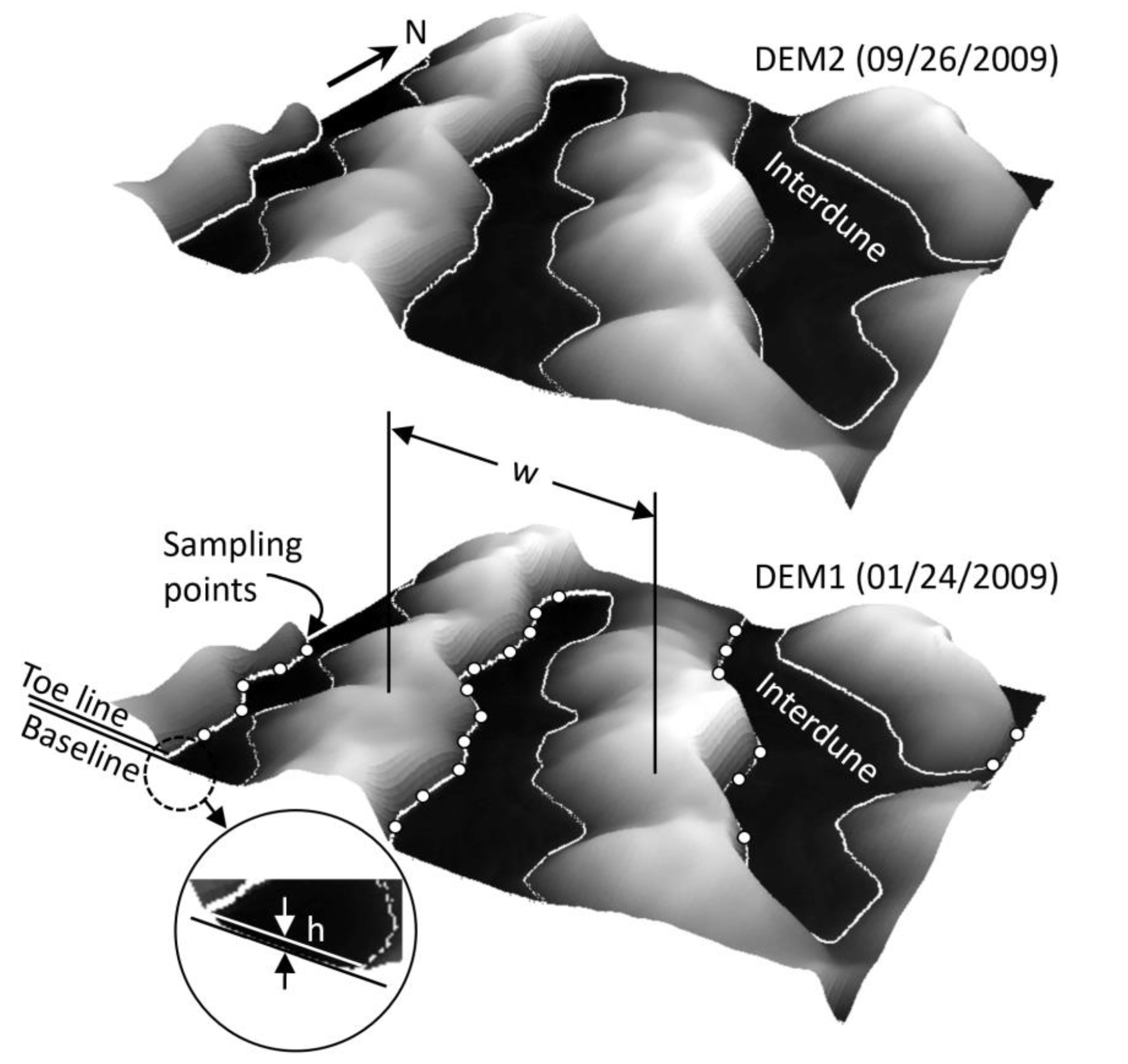
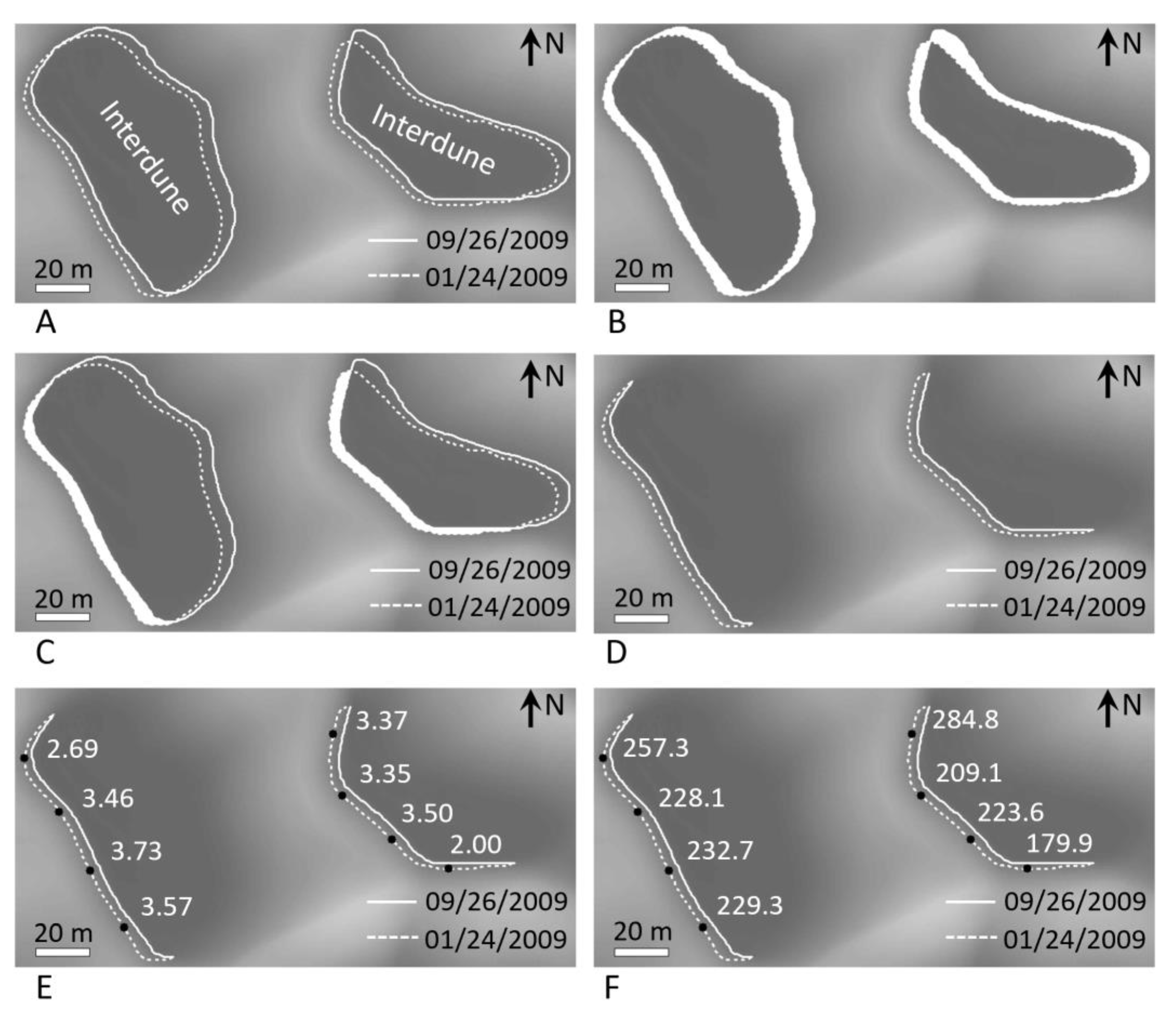
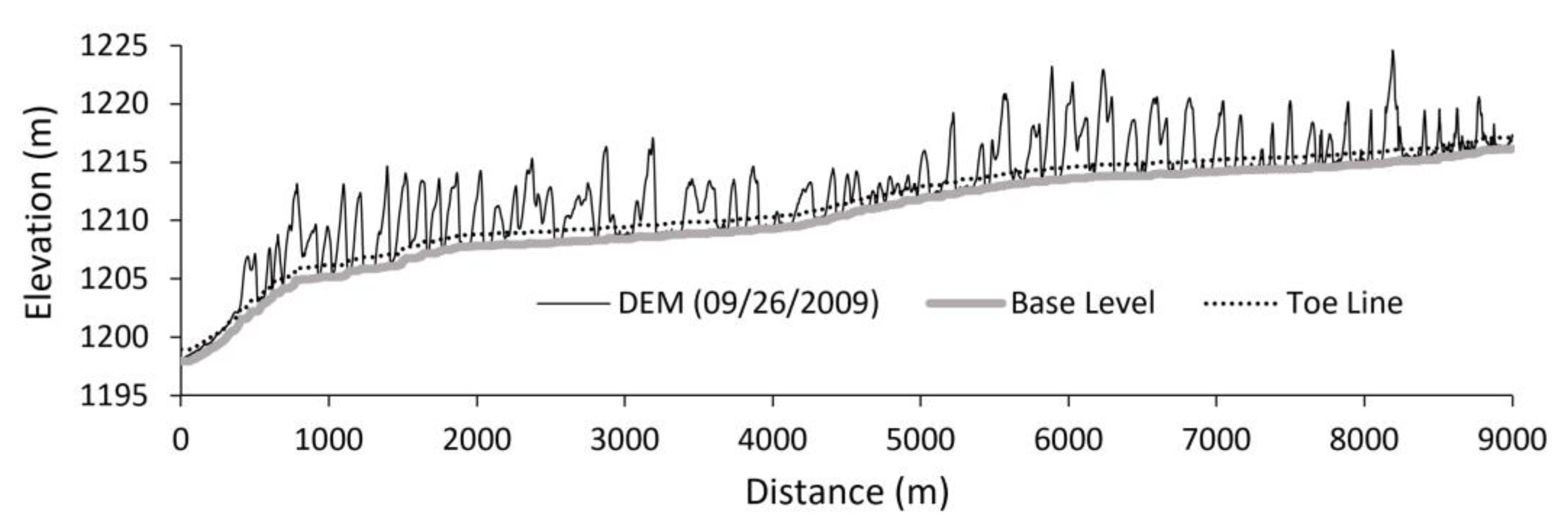
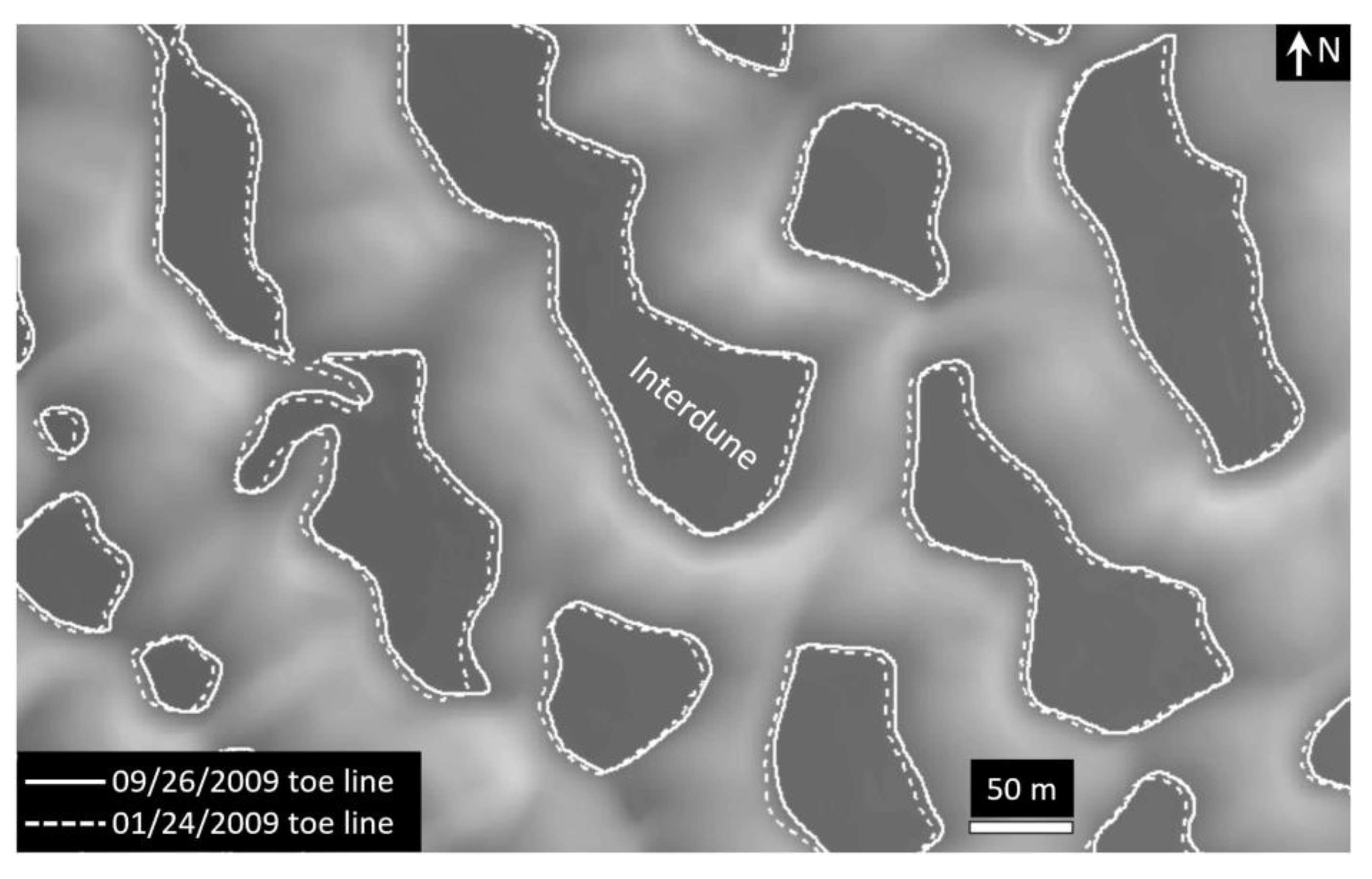
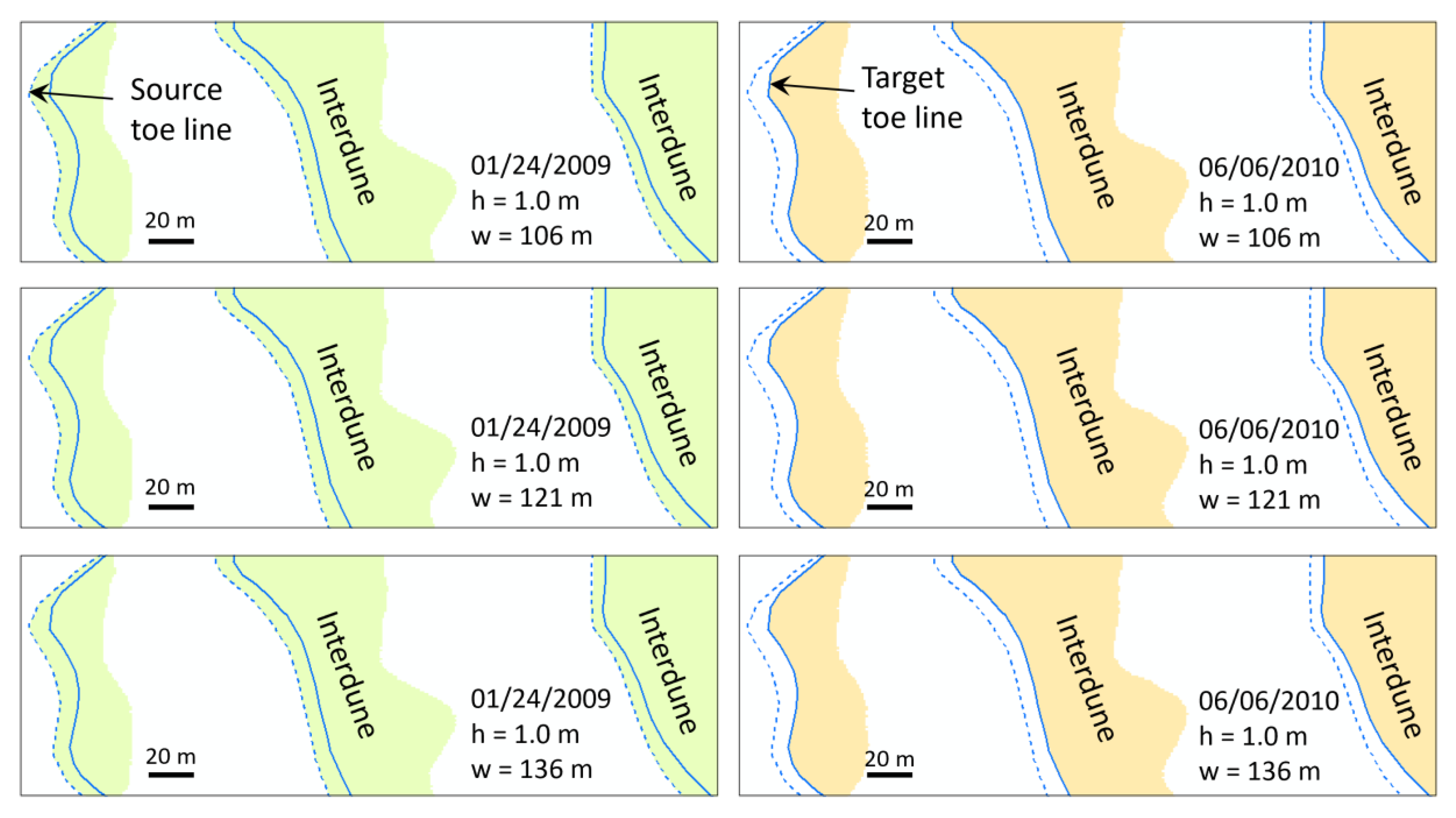
3.2. Extraction of Base Level and Toe Lines

As shown in Figure 1, reverse winds or crosswinds can modify the dune shape, and slipfaces may not be detected in DEMs using the angle of repose. The reverse winds or crosswinds can also cause sand to accumulate at the base of the dune, creating a concave-up apron (Figure 5). The point between the apron surface and the slipface (which may be modified by wind) is the toe, the area between dunes is the interdune, and the base level is a surface created from local minimum elevations of interdunes (Figure 5). For multi-temporal sand dune DEMs with or without slipfaces, the distance between two toes should provide a better approximation for the migration distance, because the dune crestline and the upper part of the leeward slope are more likely to change under reverse winds or crosswinds, while defining an identifiable point on the concave-up apron surface can be difficult. Therefore, a method is developed to extract the base level and toe lines based on the elevation of interdunes.
For an input DEM D(x, y) for sand dunes, the base level raster M(x, y) can be calculated using the minimum elevation in a w by w square window that moves across D(x, y). The user-specified window size w is determined by measuring the approximate distance between two dune crestlines (Figure 6). This is to ensure that, for any location in D(x, y), a minimum elevation in a neighboring interdune area can be used as output in M(x, y). An elevated base level raster E(x, y) is obtained by adding a constant toe height (h) to M(x, y)
E(x, y) = M(x, y) + h
The toe height h is a user-specified constant which may vary with different dune areas. However, it is not necessary to know the exact toe height in a specific dune field. It is estimated that a default h value of 1 m should work for many sand dunes. Discussion on the sensitivity of the toe height h can be found in the discussion section. Like the window size w, h can be determined by examining the 3D dune profiles.
The elevated base level raster E(x, y) can be converted to a binary raster B(x, y) showing dunes (0’s) and interdunes (1’s) by comparison with D(x, y)
B ( x , y ) = { 0 ,     D ( x , y ) > E ( x , y ) 1 ,     D ( x , y ) E ( x , y )
As shown in the flowchart (Figure 4), the binary raster B(x, y) is then converted to polygon features, and the polygons are smoothed and converted from multipart to single part to represent the toe lines. Sampling points can be generated on toe lines for the automated measurement of dune migration distance and direction (Figure 6), which is explained in the next section.

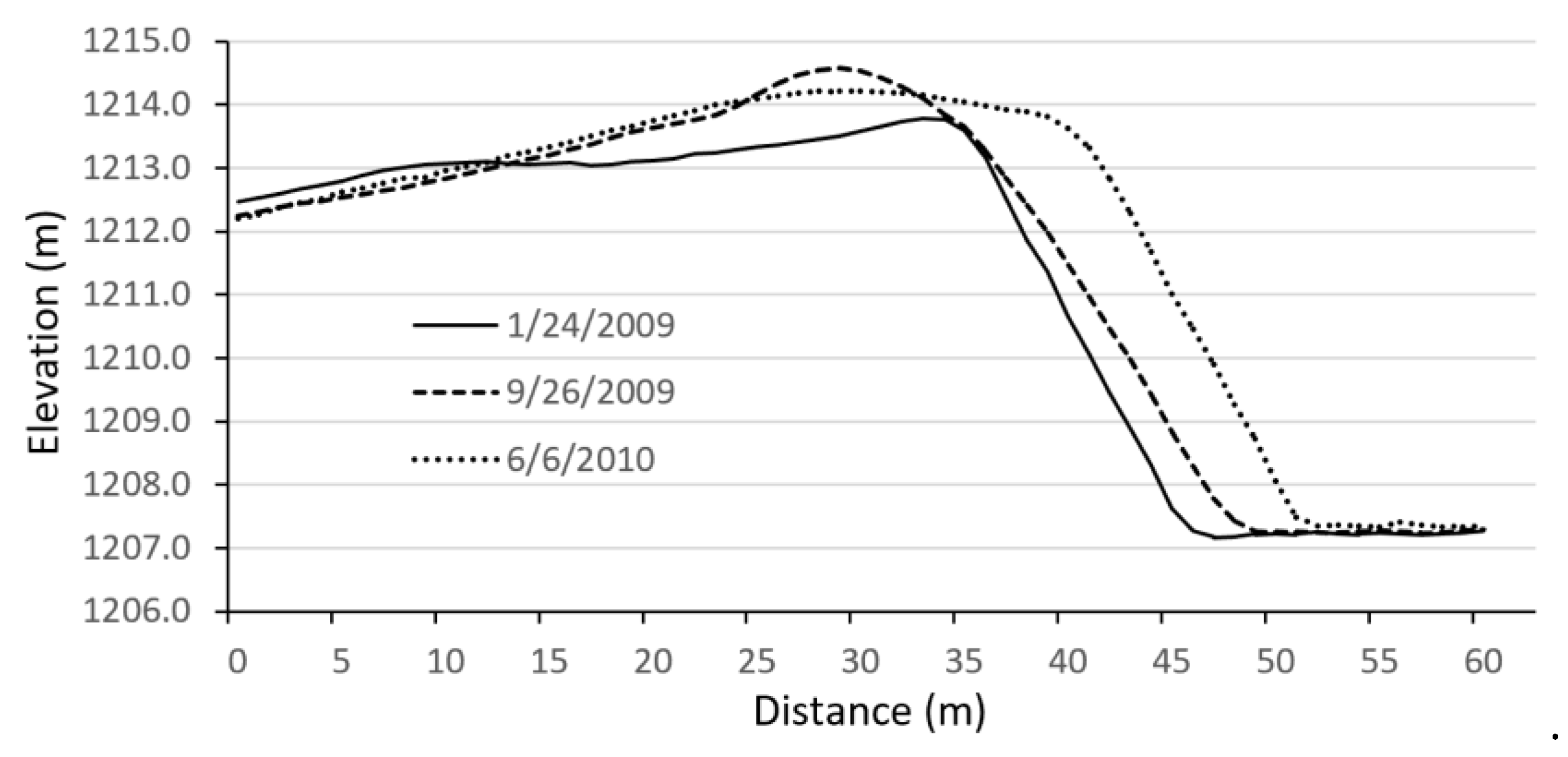
3.3. Calculation of Migration Distance and Direction

Once the toe line polygon feature classes G1 and G2 are created from two DEMs (Figure 7A), two logical operators, “AND” and “XOR”, and spatial relationships between the polygons can be used to derive source toe lines from the first DEM, and target toe lines from the second DEM. “XOR” is an exclusive “or” (or and only or) operator to produce the difference between the two polygons, while “AND” produces the intersection between the two polygons. The difference polygons K (white areas in Figure 7B) are created using
K = (G1) XOR (G2)
The multipart polygon feature class K is then converted to a single part polygon feature class L. The following three types of polygons are then removed from L: (1) small polygons with an area less than the area threshold a; (2) polygons that are not within G1; and (3) polygons that do not intersect G2. It is necessary to remove polygons that do not intersect G2, because Equation (3) may produce polygons that are part of G1 but do not intersect any polygon in G2, which may result in incorrect measurements of dune migration distance and direction. The white areas in Figure 7C show polygons in L.
The source toe lines U from the first DEM and the target toe lines V from the second DEM are created from the intersection of the polygon feature class L and the toe line polygon feature classes G1 and G2
U = (L) AND (G1)
V = (L) AND (G2)
The final source toe lines S (dashed lines in Figure 7D) and target toe lines T (solid lines in Figure 7D) are created by converting multipart lines in U and V to single part lines, respectively. Sampling points are generated on polylines in S based on the sample rate d. The distance from each sampling point to the nearest point on the target line is found using the search radius r. In the study by Yao et al. (2007), migration directions were perpendicular to the dune ridges. Similarly, migration directions in this study were calculated from the sampling points to the nearest points on the target lines. The directions are converted to the range of 0° (north) to 360°. If no nearest point is found, the distance value will be—1. Figure 7E,F show sample dune migration distances (meters) and directions (degrees) automatically calculated for sampling points on source lines. Since the number of days between the two DEMs is known, the migration distances can be further converted to migration rates (meters per year).

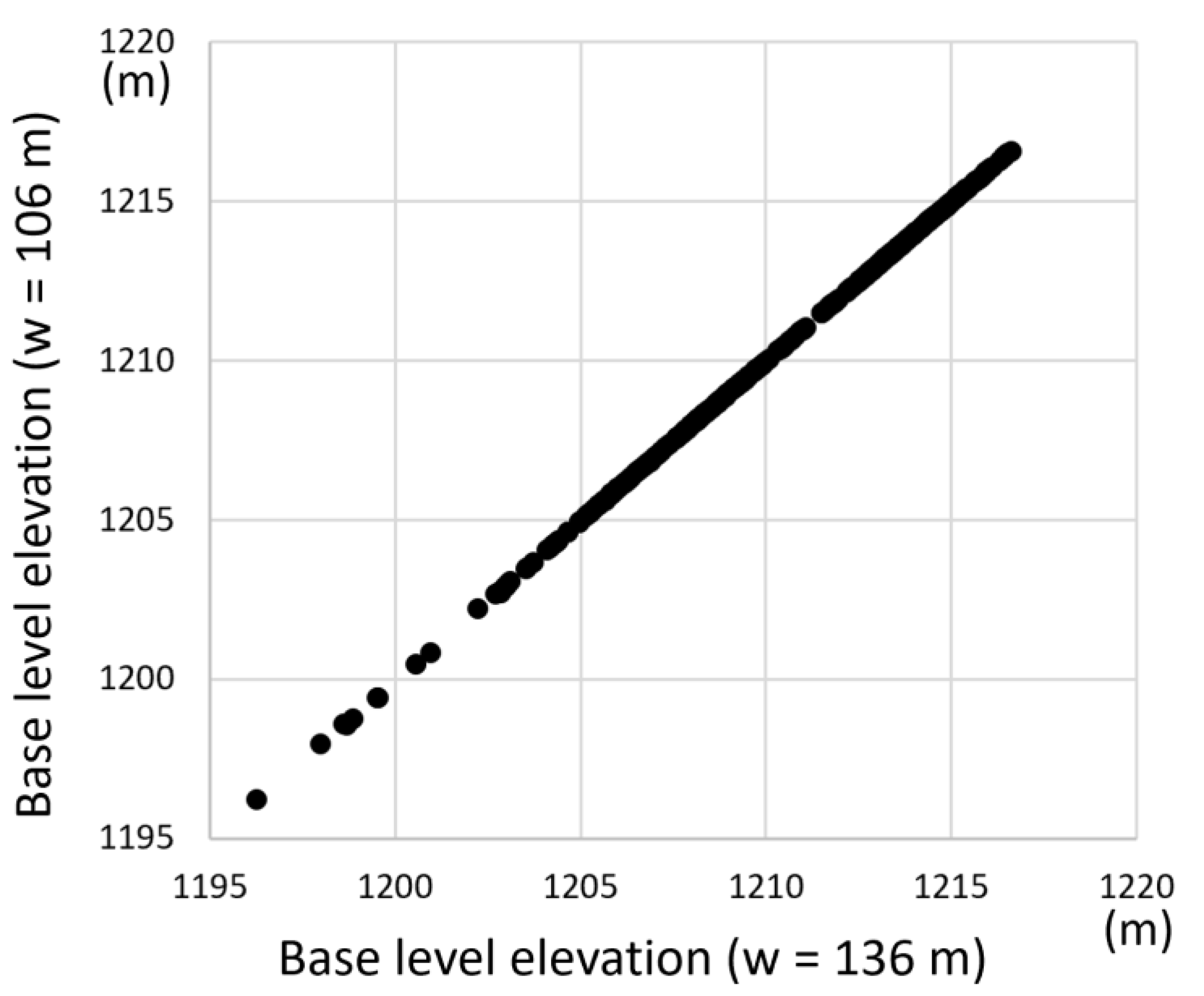
3.4. Sensitivity Analysis

Among the five user-defined parameters in the proposed method (namely window size, w; toe height, h; area threshold, a; sample rate, d; and search radius, r), the last three parameters are based on extracted toe lines, and therefore do not have major impact on the output. Three different window sizes (w) and three different toe heights (h) are tested for sensitivity analysis, and the details are presented in 5.1.

4. Results

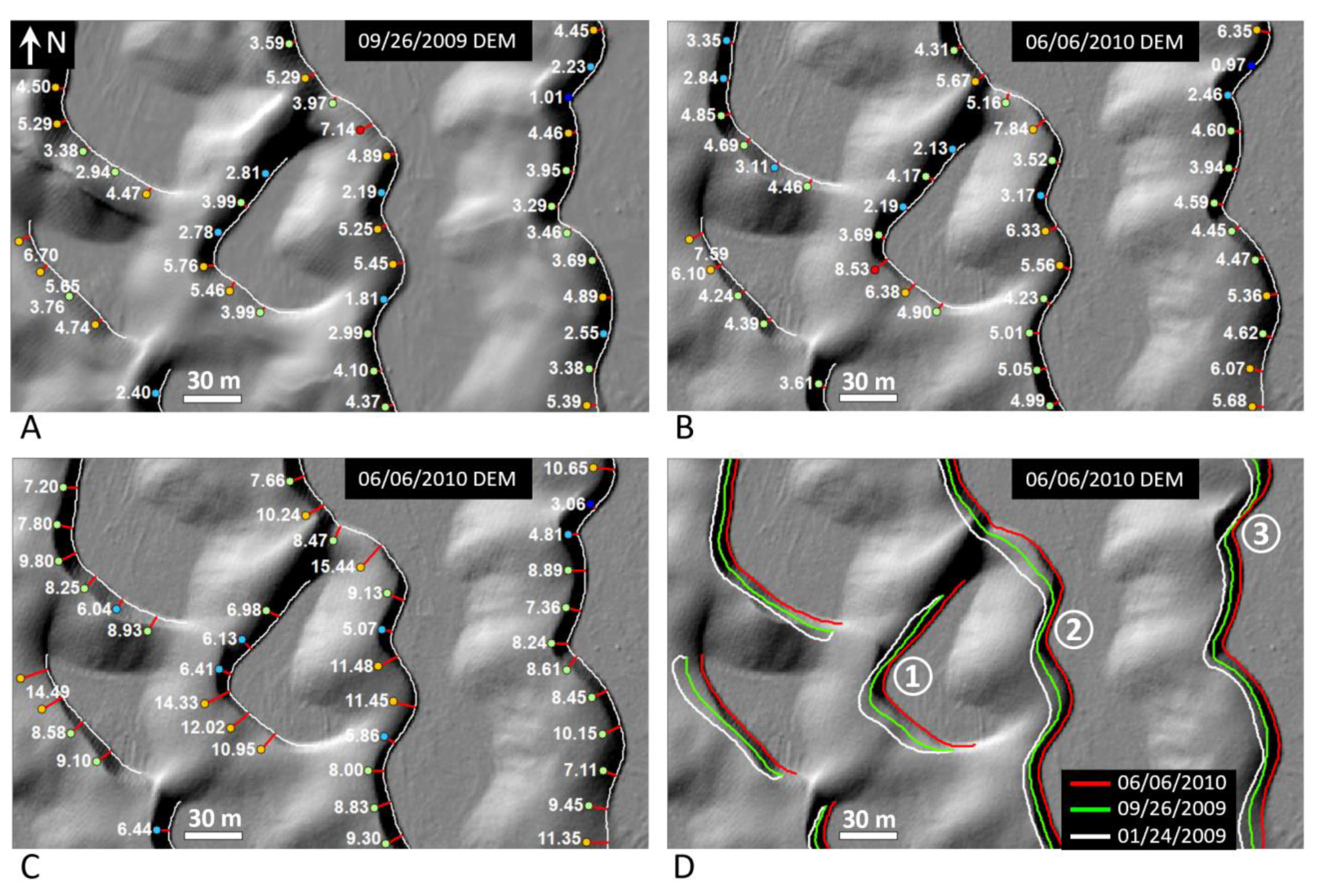
4.1. Base Level and Toe Lines

Figure 8 shows the profiles for the 26 September 2009 DEM, base level, and toe lines. The base level is obtained using a window size of 121 m by 121 m (w = 121), and the toe height is 1 m (h = 1). It can be seen that the base level matches the interdune areas very well. Figure 9 shows sample toe lines of 24 January 2009 and 26 September 2009 in the study area with a backdrop of the 26 September 2009 DEM. Figure 10 shows sample source lines derived from toe lines of 24 January 2009 with a backdrop of hillshaded DEM of 24 January 2009.

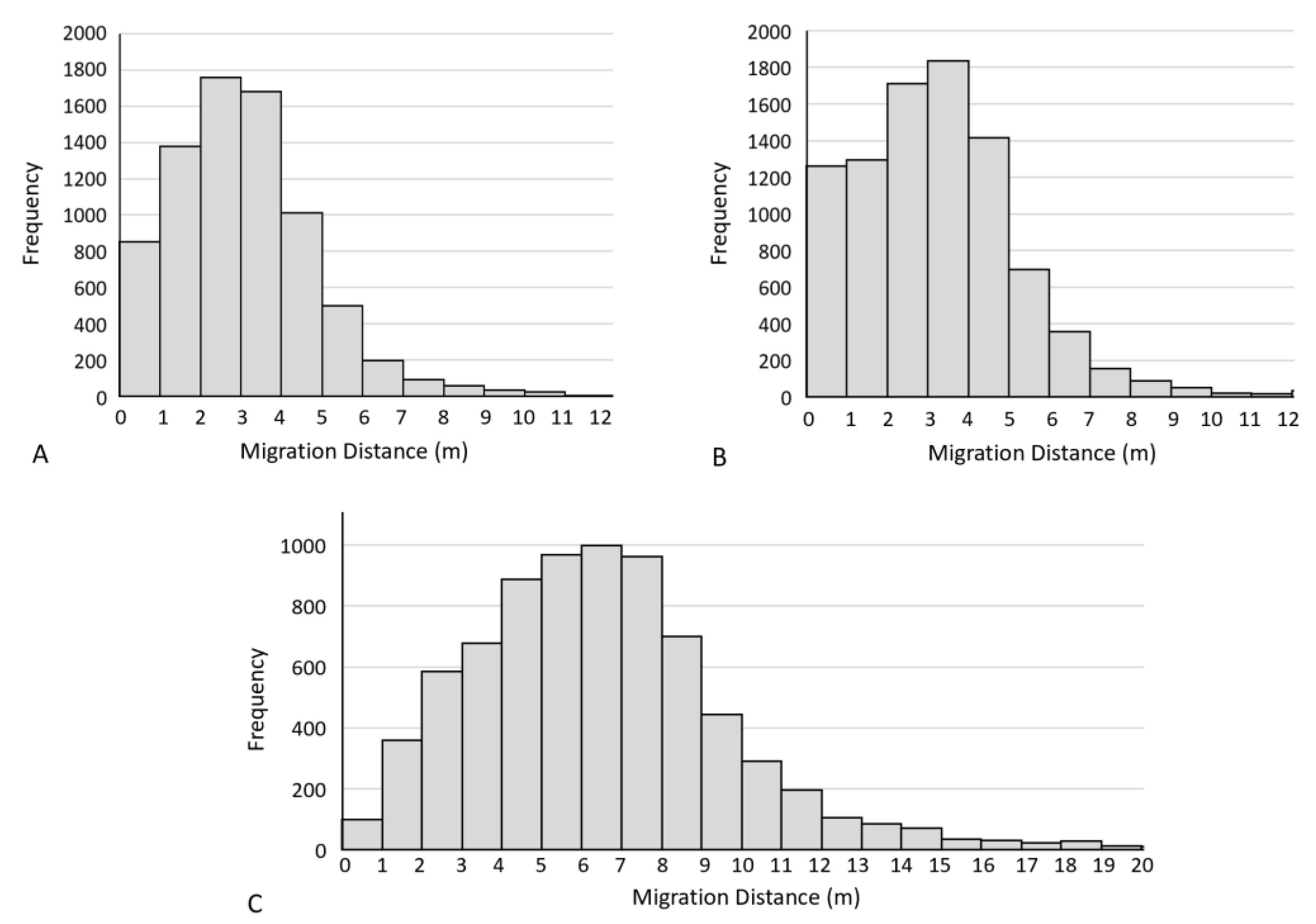
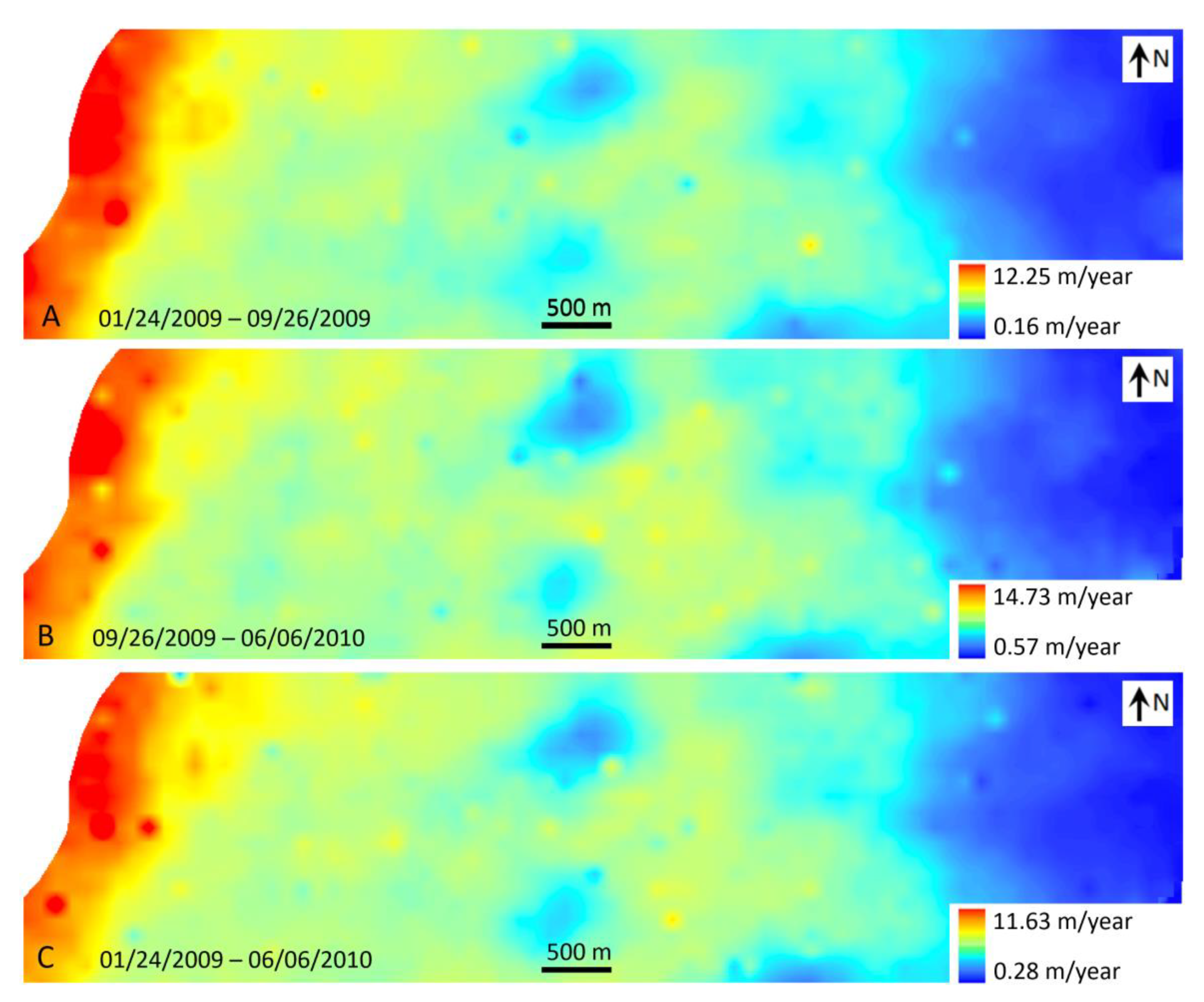
4.2. Migration Distance/Rate

The window size (w) can be estimated by measuring distances between adjacent dune ridges. Usually, the mean value of several measurements can be used as window size. The window size is a rough estimate, and does not have to be very accurate (see 5.1 for more discussion on this). Using the basic measurement tools such as distance measurement and profile generation in ArcGIS 10.7, the following parameters were estimated and employed for calculating dune migration distance and direction: w = 121 m, h = 1 m, a = 20 m2, d = 20 m, and r = 30 m. Figure 11 is a sample area showing the dune migration distances and directions from 24 January 2009 to 26 September 2009 (Figure 11A), 26 September 2009 to 6 June 2010 (Figure 11B), and 24 January 2009 to 6 June 2010 (Figure 11C). Figure 11D shows the toe line change from 24 January 2009 to 26 September 2009 to 6 June 2010. Similar to Figure 9 and Figure 10, it can be seen that the toe lines match the dune landforms very well.
To better analyze the dune migration distances, histograms are created for the migration distances for three periods: 24 January 2009 to 26 September 2009 (Figure 12A), 26 September 2009 to 6 June 2010 (Figure 12B), and 24 January 2009 to 6 June 2010 (Figure 12C). It can be seen that a majority of the migration distances are less than 6 m from 24 January 2009 to 26 September 2009, and 26 September 2009 to 6 June 2010. Since there were 498 days from 24 January 2009 to 6 June 2010, the migration distances from 24 January 2009 to 6 June 2010 (498 days) can be converted to migration rates (m/year) by multiplying the migration distance by 0.7329 (i.e., 365/498) for each sampling point. The results suggest that a majority of the sampling points have a migration rate between 3.0 m/year and 8 m/year in the study area, very similar to the results calculated from the slipfaces of 24 January 2009 and 6 June 2010 using the PSTP method [44].
The migration distances in Figure 11 can be further converted to continuous rasters for migration rates using spatial interpolation. Figure 13 is a raster map showing the dune migration rates in three periods: 24 January 2009 to 26 September 2009, 26 September 2009 to 6 June 2010, and 24 January 2009 to 6 June 2010. The rasters were created using Kriging interpolation of the migration rates for the sampling points in the study area, with a search radius of 300 m and an output cell size of 120 m. The results are very similar to the raster for migration rates created by Dong [44]: high migration rates mainly concentrate on the upwind, western edge of the dune field, whereas low migrations rates occur in the vegetated parabolic dune area which is relative stable in the east part of the study area. It seems that there are no significant changes in the spatial patterns of dune migration rates in the above three periods, although some locations may show slightly higher migration rates in the period of 26 September 2009 to 6 June 2010 compared with the other two periods. Of particular interest is the two areas with relatively low migration rates in the central part of the study area, which needs further investigation.

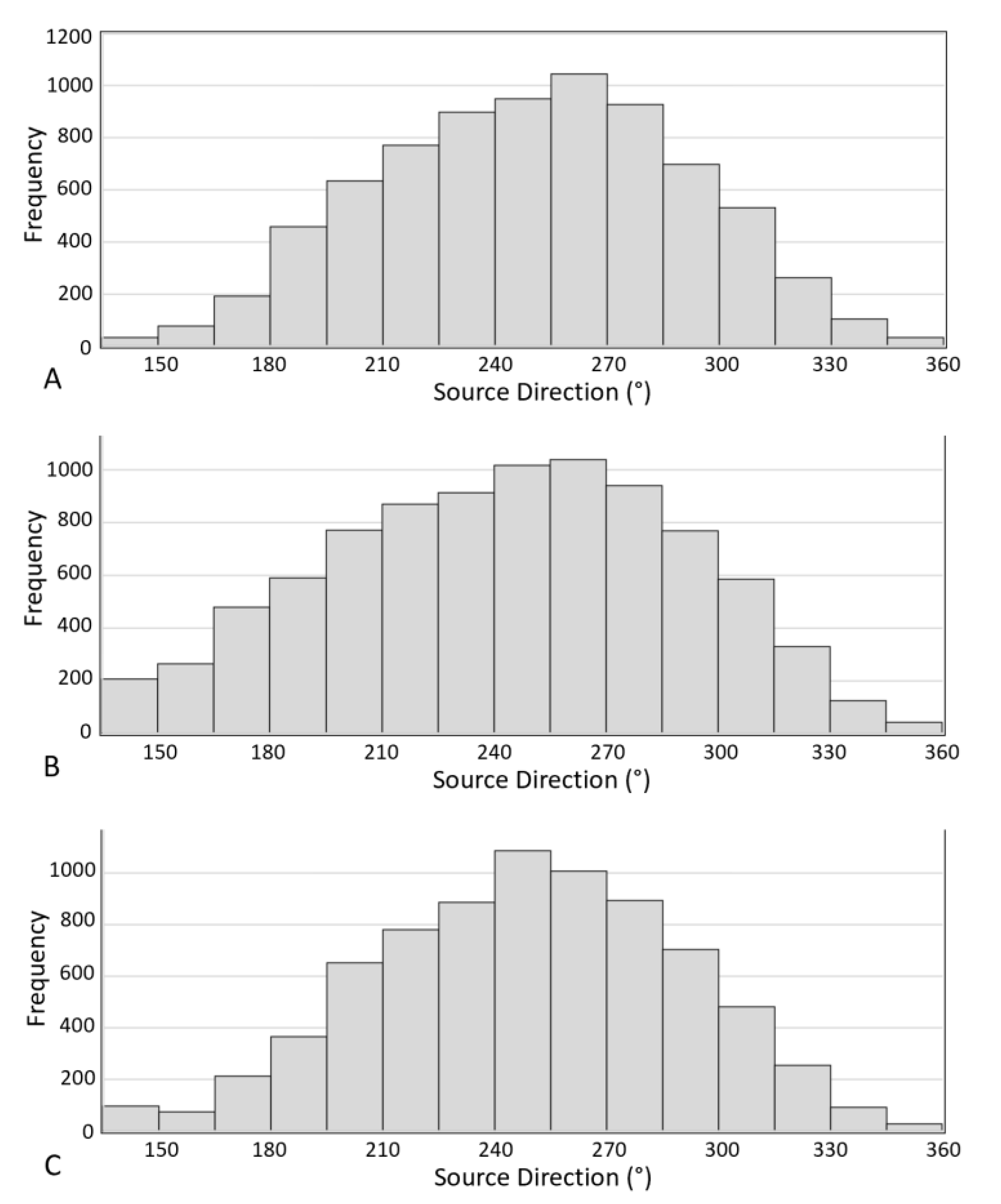
4.3. Migration Direction

Figure 14 shows the histograms of the source directions (from the source lines to the target lines), where 0° is the north. It can be seen that the migration of the toe lines is mainly from SW-W to SE-E.
The mean migration directions were calculated for three time periods: (1) 24 January 2009–26 September 2009 (7613 vectors); (2) 26 September 2009–6 June 2010 (8944 vectors); and (3) 24 January 2009–6 June 2010 (7613 vectors), with an output value of N71° E, N65° E, and N70° E, respectively. The mean migration direction of 26 September 2009 to 6 June 2010 was slightly to the north compared with that of the other two periods, suggesting that the regional wind regime changed in the second time period (26 September 2009 to 6 June 2010). However, it should be noted these mean migration directions are calculated from the migration directions of the toe lines, and do not represent the mean wind direction. In fact, reverse winds can change the dune crestlines but do not change the toe lines in the reverse direction in most cases (also see Figure 1). The relationship between the dune migration direction and the wind directions can be more complex. For example, the narrow intervals between the toe lines at ①, ②, and ③ in Figure 11D could be caused by wind flows not perpendicular to the migration direction, as discussed in Tsoar et al. [52].

5. Discussion

5.1. Sensitivity Analysis

As explained in 3.1, there are five user-defined parameters in the proposed method: window size (w), toe height (h), area threshold (a), sample rate (d), and search radius (r). The last three parameters do not have major impact on the output because they are based on the extracted toe lines. However, window size (w) and toe height (h) may affect the binary rasters (B1 and B2 in Figure 4) that control the output toe lines. The results in previous sections were obtained using w = 121 m and h = 1.0 m. For sensitivity analysis, four additional experiments were carried out for the two DEMs for 24 January 2009 and 6 June 2010: (1) w = 106 m, (2) w = 136 m, (3) h = 0.5 m, and (4) h = 1.5 m, while the other parameters remain the same (a = 20 m2, d = 20 m, and r = 30 m).
Figure 15 shows interdune areas derived from the 24 January 2009 and 6 June 2010 DEMs using the TLT method, with h = 1.0 m and w = 106 m, 121 m, and 136 m. The source toe lines (dashed lines) and target toe lines (solid lines) obtained using w = 121 m are also shown as reference. When the window size w changes from 106 m to 121 m to 136 m. It can be seen that identical toe lines can be obtained using the TLT method. There are only minor changes in the raster cells along the borders of interdune areas, which are smoothed during raster to polygon conversion. Such results are not surprising, because the base level rasters are obtained by calculating the minimum elevations in the w × w windows, following by calculating the mean values in the w × w windows. As a result, different window sizes, such as 106 × 106, 121 × 121, and 136 × 136, may produce very close base level rasters. To show the similarities between the base levels generated using different window sizes, 384 random points were generated in the study area to extract elevations from the three base level rasters. Figure 16 shows the scatter diagram between the base level rasters obtained using w = 106 m and 136 m, respectively. It can be seen that the two base level rasters are almost identical. The results suggest that an estimated average distance between sand dune ridges can be used as the window size, and that average distance does not have to be very accurate.
Figure 17 shows the source toe lines and target toe lines using 1.0 m and 1.5 m as the toe height (h), with interdune areas of h = 0.5 m as the background. It can be seen that the extracted toe lines are very close when h = 0.5, 1.0, and 1.5 m. The similarities in output toe lines can be explained using basic trigonometry: suppose the leeward slope is 30°, when the toe height h increases from 1.0 m to 1.5 m, the horizontal shift of the toe line is 0.5/tan(30°) = 0.87 m. Since the DEM cell size is 1 m, minor horizontal shifts (less than 1 m) in the toe line can results in the same polyline after raster to polygon conversion and polygon smoothing.
To get a better picture of the toe line variations with different toe heights in the whole study area, the following two tests were conducted: (1) A total of 2670 random sampling points were generated on source toe lines (h = 1.0 m), and a radius of 3 m around each sampling point was used to search the nearest point on the source toe lines (h = 1.5 m) and measure the distance (DIST1). (2) Similarly, a total of 2297 random sampling points were generated on target toe lines (h = 1.0 m) to measure the distances (DIST2) from each point the nearest target toe lines (h = 1.5 m). In other words, random points were generated to measure distances between the two dashed lines (DIST1) and between the two solid lines (DIST2) in Figure 16 over the whole study area. The results are summarized in Table 1.
Table 1 shows that almost 90% of toe line points are within 2 m when toe height changes from 1.0 m to 1.5 m, while a majority of them (>60%) are within 1 m. It should be noted that such displacements in toe lines caused by toe height change do not necessarily mean changes in migration distances, because both the source toe line and the target toe line usually change in the same direction as shown in Figure 17, maintaining a relatively stable distance. The results suggest that the toe height (h) change does not significantly affect the dune migration measurements, as long as h is not very low (close to the vertical accuracy of LiDAR data) and not very high (for example, less than 1.5 m so that small dunes can also be measured). A toe height of 1 m should work for measurement of many dune fields.

5.2. Limitations

Like the PSTP method, the application of the TLT method can be affected by dune form, dune interaction, dune migration rate, and data acquisition interval. The TLT method can be used for barchan, barchanoid ridge, transverse dunes, and even linear dunes, but cannot be directly applied to star dunes where the complex wind regime creates multiple slopes. Depending on the migration rates of a dune field, the TLT method may not be suitable for measuring dune migration distance and direction if two datasets are acquired with a substantial time interval (e.g., several years) for a fast-moving dune field, because dune interaction during migration may involve complex changes in dune shape. It is hoped that terrestrial (stationary or mobile) and unmanned aerial vehicle (UAV) LiDAR systems can provide new options for monitoring sand dune changes.

6. Conclusions

Automated or semi-automated change detection of large dune fields is a challenging problem. After reviewing the limitation of the existing PSTP method for measuring sand dune migration rate and migration direction, this paper introduced a toe line tracking (TLT) method and implemented the new method using the Python programming language for automated measurement of dune migration distance and direction based on multi-temporal LiDAR-derived DEMs. Using a few simple parameters, the TLT method automatically extracts the base level of a dune field and toe lines of individual dunes. The toe line polygons derived from two DEMs are processed using logical operators and other spatial analysis methods in a geographic information system, and source toe lines and target toe lines are extracted from the toe line polygons.
The application of the TLT method was demonstrated using multi-temporal LiDAR-derived DEMs for a 9 × 2.4 km area in the White Sands Dune Field in New Mexico (USA). By generating over 7000 random sampling points along source toe lines, dune migration distances and directions are calculated and analyzed. Dune migration distances and directions for three periods (24 January 2009 to 26 September 2009, 26 September 2009 to 6 June 2010, and 24 January 2009 to 6 June 2010) were calculated. The migration distances can be further converted into migration rates. The dune migration rates for the study area obtained from the TLT method for the periods of 24 January 2009 to 26 September 2009, 26 September 2009 to 6 June 2010, and 24 January 2009 to 6 June 2010 show very similar spatial patterns. Sensitivity analyses were carried out using different window sizes (106, 121, and 136 m) and toe heights (0.5, 1.0, and 1.5 m). The results suggest that the TLT method is relatively insensitive to changes in window size. Although a toe height of 0.5 m (which is close to the vertical accuracy of LiDAR data, 0.35 m, in this study) does not work well in some areas due to elevation variations near the interdune surfaces and presence of shrubs, a toe height between 1.0 to 1.5 m can produce very close outputs, as shown in statistics from thousands of sampling points. The results show that TLT is a more generic method than PSTP in that it works for dunes with or without slipfaces that reach the angle of repose, and can be used for effective measurement of dune migration distance/rate and direction in large dune fields.

Author Contributions

Conceptualization, P.D. and J.X.; Methodology, P.D., J.X., and R.Z.; Software, P.D.; Validation, R.Z., Z.Z., S.T., and J.X.; Writing—original draft preparation, P.D.; Writing—review and editing, P.D., J.X., R.Z., Z.Z., and S.T.; Project administration, J.X. and P.D. All authors have read and agreed to the published version of the manuscript.

Funding

J.X.’s research was funded by (National Natural Science Foundation of China) grant number (42061038).

Institutional Review Board Statement

Not applicable.

Informed Consent Statement

Not applicable.

Data Availability Statement

The LiDAR datasets are downloaded from the official website of OpenTopography: https://opentopography.org/ (accessed on 2 March 2015).

Conflicts of Interest

The authors declare no conflict of interest.

References

  1. Bagnold, R.A. The Physics of Blown Sand and Desert Dunes; Chapman and Hall: London, UK, 1941; p. 265. [Google Scholar]
  2. Wasson, R.; Hyde, R. Factors determining desert dune type. Nature 1983, 304, 337–339. [Google Scholar] [CrossRef]
  3. Lancaster, N. Geomorphology of Desert Dunes; Routledge: London, UK, 1995; p. 312. [Google Scholar]
  4. Fenton, L.K. Dune migration and slip face advancement in the Rabe Crater dune field, Mars. Geophys. Res. Lett. 2006, 33, L20201. [Google Scholar] [CrossRef]
  5. Hugenholtz, C.H.; Wolfe, S.A.; Moorman, B.J. Sand-water flows on cold-climate eolian dunes: Environmental analogs for the eolian rock record and Martian sand dunes. J. Sediment. Res. 2007, 77, 1–8. [Google Scholar] [CrossRef]
  6. Rubin, D.; Hesp, P.A. Multiple origins of linear dunes on Earth and Titan. Nat. Geosci. 2009, 2, 653–658. [Google Scholar] [CrossRef]
  7. Bourke, M.C.; Lancaster, N.; Fenton, L.K.; Parteli, E.J.R.; Zimbelman, J.R.; Radebaugh, J. Extraterrestrial dunes: An introduction to the special issue on planetary dune systems. Geomorphology 2010, 121, 1–14. [Google Scholar] [CrossRef]
  8. Bridges, N.T.; Ayoub, F.; Avouac, J.-P.; Leprince, S.; Lucas, A.; Mattson, S. Earth-like sand fluxes on Mars. Nature 2012, 485, 339–342. [Google Scholar] [CrossRef] [PubMed] [Green Version]
  9. Livingstone, I.; Wiggs, G.F.S.; Weaver, C.M. Geomorphology of desert sand dunes: A review of recent progress. Earth Sci. Rev. 2007, 80, 239–257. [Google Scholar] [CrossRef]
  10. Rubin, D.M. Lateral migration of linear dunes in the Strzelecki Desert, Australia. Earth Surf. Process. Landf. 1990, 15, 11–14. [Google Scholar] [CrossRef]
  11. Ha, S.; Dong, G.; Wang, G. Morphodynamic study of reticulate dunes at southeastern fringe of the Tengger Desert. Sci. China 1999, 42, 207–215. [Google Scholar] [CrossRef]
  12. Dong, Z.; Wang, X.; Chen, G. Monitoring sand dune advance in the Taklimakan Desert. Geomorphology 2000, 35, 219–231. [Google Scholar] [CrossRef]
  13. Dong, Z.; Wang, T.; Wang, X. Geomorphology of the megadunes in the Badain Jaran Desert. Geomorphology 2004, 60, 191–203. [Google Scholar] [CrossRef]
  14. Elbelrhiti, H.; Claudin, P.; Andreotti, B. Field evidence for surface-wave-induced instability of sand dunes. Nature 2005, 437, 720–723. [Google Scholar] [CrossRef]
  15. Ewing, R.C.; Kocurek, G. Aeolian dune-field pattern boundary conditions. Geomorphology 2010, 114, 175–187. [Google Scholar] [CrossRef]
  16. Narteau, C.; Zhang, D.; Rozier, O.; Claudin, P. Setting the length and timescales of a cellular automaton dune model from the analysis of superimposed bed forms. J. Geophys. Res. 2009, 114, F03006. [Google Scholar]
  17. Zhang, D.; Narteau, C.; Rozier, O. Morphodynamics of barchan and transverse dunes using a cellular automaton model. J. Geophys. Res. 2010, 115, F03041. [Google Scholar] [CrossRef]
  18. Barrio-Parra, F.; Rodríguez-Santalla, I. A free cellular model of dune dynamics: Application to El Fangar spit dune system (Ebro Delta, Spain). Comput. Geosci. 2014, 62, 187–197. [Google Scholar] [CrossRef]
  19. Alhajraf, S. Computational fluid dynamic modeling of drifting particles at porous fences. Environ. Model. Softw. 2004, 19, 163–170. [Google Scholar] [CrossRef]
  20. Hersen, P. On the crescentic shape of barchans dunes. Eur. Phys. J. B 2004, 37, 507–514. [Google Scholar] [CrossRef] [Green Version]
  21. Araújo, A.D.; Parteli, E.J.R.; Pöschel, T.; Andrade, J.S.; Herrmann, H.J. Numerical modeling of the wind flow over a transverse dune. Sci. Rep. 2013, 3, 2858. [Google Scholar] [CrossRef] [PubMed] [Green Version]
  22. Gay, S.P. Observations regarding the movement of barchan sand dunes in the Nazca to Tanaca area of southern Peru. Geomorphology 1999, 27, 279–293. [Google Scholar]
  23. Jimenez, J.A.; Maia, L.P.; Serra, J.; Morias, J. Aeolian dune migration along the Ceara coast, north-eastern Brazil. Sedimentology 1999, 46, 689–701. [Google Scholar] [CrossRef]
  24. Bailey, S.D.; Bristow, C.S. Migration of parabolic dunes at Abberffraw, Anglesey, north Wales. Geomorphology 2004, 59, 165–174. [Google Scholar] [CrossRef]
  25. Levin, N.; Ben-Dor, E.; Karnieli, A. Topographic information of sand dunes as extracted from shading effects using Landsat images. Remote. Sens. Environ. 2004, 90, 190–209. [Google Scholar] [CrossRef]
  26. Leprince, S.; Barbot, S.; Ayoub, F.; Avouac, J. Automatic and precise orthorectification, coregistration, and subpixel correlation of satellite images, application to ground deformation measurements. IEEE Trans. Geosci. Remote Sens. 2007, 45, 1529–1558. [Google Scholar] [CrossRef] [Green Version]
  27. Yao, Z.Y.; Wang, T.; Han, Z.W.; Zhang, W.M.; Zhao, A.G. Migration of sand dunes on the northern Alxa Plateau, Inner Mongolia, China. J. Arid Environ. 2007, 70, 80–93. [Google Scholar] [CrossRef]
  28. Vermeesch, P.; Drake, N. Remotely sensed dune celerity and sand flux measurements of the world’s fastest barchans (Bodélé, Chad). Geophys. Res. Lett. 2008, 35, L24404. [Google Scholar] [CrossRef] [Green Version]
  29. Necsoiu, M.; Leprince, S.; Hooper, D.M.; Dinwiddie, C.L.; McGinnis, R.N.; Walter, G.R. Monitoring migration rates of an active subarctic dune field using optical imagery. Remote Sens. Environ. 2009, 113, 2441–2447. [Google Scholar] [CrossRef]
  30. Mohamed, I.N.L.; Verstraeten, G. Analyzing dune dynamics at the dune-field scale based on multi-temporal analysis of Landsat-TM images. Remote Sens. Environ. 2012, 119, 105–117. [Google Scholar] [CrossRef]
  31. Mitasova, H.; Hardin, E.; Starek, M.J.; Harmon, R.S.; Overton, M.F. Landscape dynamics from LiDAR data time series. In Geomorphometry; Hengl, T., Evans, I.S., Wilson, J.P., Gould, M., Eds.; Geomorphometry.org: Redlands, CA, USA, 2011; pp. 3–6. [Google Scholar]
  32. Solazzo, D.; Sankey, J.B.; Sankey, T.T.; Munson, S.M. Mapping and measuring aeolian sand dunes with photogrammetry and LiDAR from unmanned aerial vehicles (UAV) and multispectral satellite imagery on the Paria Plateau, AZ, USA. Geomorphology 2018, 319, 174–185. [Google Scholar] [CrossRef]
  33. Grohmann, C.H.; Garcia, G.P.B.; Affonoso, A.A.; Albuquerque, R.W. Dune migration and volume change from airborne LiDAR, terrestrial LiDAR and Structure from Motion-Multi View Stereo. Comput. Geosci. 2020, 143, 1–13. [Google Scholar] [CrossRef]
  34. Ding, C.; Zhang, L.; Liao, M.; Feng, G.; Dong, J.; Ao, M.; Yu, Y. Quantifying the spatio-temporal patterns of dune migration near Minqin Oasis in northwestern China with time series of Landsat-8 and Sentinel-2 observations. Remote Sens. Environ. 2020, 236, 1–24. [Google Scholar] [CrossRef]
  35. Ali, E.; Xu, W.; Ding, X. Improved optical image matching time series inversion approach for monitoring dune migration in North Sinai Sand Sea: Algorithm procedure, application, and validation. ISPRS J. Photogramm. Remote Sens. 2020, 164, 106–124. [Google Scholar] [CrossRef]
  36. Goudie, A. Geomorphological Techniques, 2nd ed.; Routledge: London, UK, 1994; p. 570. [Google Scholar]
  37. Woolard, J.W.; Colby, J.D. Spatial characterization, resolution, and volumetric change of coastal dunes using airborne LIDAR: Cape Hatteras, North Carolina. Geomorphology 2002, 48, 269–287. [Google Scholar] [CrossRef] [Green Version]
  38. Hardin, E.; Mitasova, H.; Tateosian, L.G.; Overton, M. GIS-Based Analysis of Coastal Lidar Time-Series, Springer Briefs in Computer Science. Available online: https://0-link-springer-com.brum.beds.ac.uk/book/10.1007/978-1-4939-1835-5 (accessed on 28 June 2021).
  39. Saye, S.E.; van der Wal, D.; Pye, K.; Blott, S.J. Beach–dune morphological relationships and erosion/accretion: An investigation at five sites in England and Wales using LIDAR data. Geomorphology 2005, 72, 128–155. [Google Scholar] [CrossRef]
  40. Reitz, M.D.; Jerolmack, D.J.; Ewing, R.C.; Martin, R.L. Barchan-parabolic dune pattern transition from vegetation stability threshold. Geophys. Res. Lett. 2010, 37, L19402. [Google Scholar] [CrossRef] [Green Version]
  41. Ewing, R.C.; Kocurek, G.A. Aeolian dune interactions and dune-field pattern formation: White Sands Dune Field, New Mexico. Sedimentology 2010, 57, 1199–1219. [Google Scholar] [CrossRef]
  42. Baitis, E.; Kocurek, G.; Smith, V.; Mohrig, D.; Ewing, R.C.; Peyret, A.-P.B. Definition and origin of the dune-field pattern at White Sands, New Mexico. Aeolian Res. 2014, 15, 269–287. [Google Scholar] [CrossRef]
  43. Ewing, R.C.; McDonald, G.D.; Hayes, A.G. Multi-spatial analysis of aeolian dune-field patterns. Geomorphology 2015, 240, 44–53. [Google Scholar] [CrossRef]
  44. Dong, P. Automated measurement of sand dune migration using multi-temporal LiDAR data and GIS. Int. J. Remote Sens. 2015, 36, 5526–5547. [Google Scholar] [CrossRef]
  45. Hugenholtz, C.H.; Levin, N.; Barchyn, T.E.; Baddock, M. Remote sensing and spatial analysis of aeolian sand dunes: A review and outlook. Earth Sci. Rev. 2012, 111, 319–334. [Google Scholar] [CrossRef]
  46. Okyay, U.; Telling, J.; Glennie, C.L.; Dietrich, W.E. Airborne lidar change detection: An overview of Earth sciences applications. Earth Sci. Rev. 2019, 198, 1–25. [Google Scholar] [CrossRef]
  47. Xia, J.; Dong, P. A GIS add-in for automated measurement of sand dune migration using LiDAR-derived multi-temporal and high-resolution digital elevation models. Geosphere 2016, 12, 1316–1322. [Google Scholar] [CrossRef]
  48. Kocurek, G.; Carr, M.; Ewing, R.; Havholm, K.G.; Nagar, Y.C.; Singhvi, A.K. White Sands Dune Field, New Mexico: Age, dune dynamics and recent accumulations. Sediment. Geol. 2007, 197, 313–331. [Google Scholar] [CrossRef]
  49. McKee, E. Structures of dunes at White Sands National Monument, New Mexico (and a comparison with structures of dunes from other selected areas). Sedimentology 1966, 7, 1–69. [Google Scholar] [CrossRef]
  50. Langford, R.P. The Holocene history of the White Sands dune field and influences on eolian deflation and playa lakes. Quat. Int. 2003, 104, 31–39. [Google Scholar] [CrossRef]
  51. Ewing, R.C.; Kocurek, G.; Lake, L.W. Pattern analysis of dune-field parameters. Earth Surf. Process. Landf. 2006, 31, 1176–1191. [Google Scholar] [CrossRef]
  52. Tsoar, H.; Blumberg, D.G.; Stoler, Y. Elongation and migration of sand dunes. Geomorphology 2004, 57, 293–302. [Google Scholar] [CrossRef]
Figure 1. Three west–east profiles of a dune in WSDF extracted from LiDAR-derived DEMs of 24 January 2009; 26 September 2009; and 6 June 2010.
Remotesensing 13 03084 g001
Figure 2. Location of study area shown as a point (left) and a black rectangle (right) over a Landsat TM image acquired on 14 June 2010 and displayed as color composite of bands 5(R), 4(G), and 3(B) (from Dong [44]).
Remotesensing 13 03084 g002
Figure 3. Multi-temporal LiDAR-derived DEMs of the study area (2.4 × 9 km) in White Sands, New Mexico, USA.
Remotesensing 13 03084 g003
Figure 4. Flowchart for the toe line tracking (TLT) method.
Remotesensing 13 03084 g004
Figure 5. Some elements of a barchan dune.
Remotesensing 13 03084 g005
Figure 6. Window size (w) and toe height (h) in a DEM for dunes.
Remotesensing 13 03084 g006
Figure 7. Major steps for calculating dune migration distance and directions. (A) Toe line polygons extracted from 24 January 2009 and 26 September 2009 DEMs. (B) Differences (white areas) between toe line polygons. (C) Differences (white areas) that are within the 24 January 2009 toe line polygons. (D) Source toe lines (24 January 2019) and target toe lines (26 September 2009) derived from toe line polygons. (E) Dune migration distances (meters) automatically calculated for sampling points on source lines. (F) Source direction from 0 (north) to 360° automatically calculated from sampling points on source lines to nearest points on target lines. The background is the 26 September 2009 DEM.
Remotesensing 13 03084 g007
Figure 8. West-east central profiles for the DEM (26 September 2009), base level, and toe lines. The base level was obtained using a window size of 121 m by 121 m, and the toe height is 1 m.
Remotesensing 13 03084 g008
Figure 9. Sample toe lines of 24 January 2009 and 26 September 2009 in the study area with a backdrop of the 26 September DEM.
Remotesensing 13 03084 g009
Figure 10. Sample source toe lines (dashed) derived from toe lines of 24 January 2009 with a backdrop of hillshaded DEM of 24 January 2009.
Remotesensing 13 03084 g010
Figure 11. Sample area showing the dune migration distances (in meters) and directions from 24 January 2009 to 26 September 2009 (A); 26 September 2009 to 6 June 2010 (B); and 24 January 2009 to 6 June 2010 (C). The toe line changes are shown in (D). The backdrops are shaded DEMs. The point colors represent different levels of dune migration distance on that map.
Remotesensing 13 03084 g011
Figure 12. Histograms for dune migration distances. (A) 24 January 2009 to 26 September 2009; (B) 26 September 2009 to 6 June 2010; and (C) 24 January 2009 to 6 June 2010.
Remotesensing 13 03084 g012
Figure 13. Raster maps created using Kriging interpolation (search radius: 300 m, cell size: 120 m) to show the spatial distribution of dune migration rates from (A) 24 January 2009 to 26 September 2009; (B) 26 September 2009 to 6 June 2010; and (C) 24 January 2009 to 6 June 2010.
Remotesensing 13 03084 g013
Figure 14. Histograms of the source directions (from the source lines to the target lines), where 0° is the north. (A) 24 January 2009 to 26 September 2009 (7613 vectors); (B) 26 September 2009 to 6 June 2010 (8944 vectors); and (C) 24 January 2009 to 6 June 2010 (7613 vectors).
Remotesensing 13 03084 g014
Figure 15. Interdune areas derived from the 24 January 2009 and 6 June 2010 DEMs using the TLT method, with h = 1.0 m and w = 106 m, 121 m, and 136 m, respectively. The source toe lines (dashed lines) and target toe lines (solid lines) obtained using w = 121 m are also shown as reference.
Remotesensing 13 03084 g015
Figure 16. Scatter diagram between base level elevations obtained using w = 106 m and 136 m.
Remotesensing 13 03084 g016
Figure 17. Source toe lines and target toe lines obtained using different toe heights.
Remotesensing 13 03084 g017
Table 1. Statistics of distances between source toe lines (DIST1) and between target toe lines (DIST2).
Mean
Distance (m)
Standard
Deviation (m)
No. of Distances within 1.0 mNo. of Distances within 2.0 m
DIST11.110.58851612/2670 (60.4%)2379/2670 (89.1%)
DIST21.100.59091439/2297 (62.6%)2048/2297 (89.2%)
Publisher’s Note: MDPI stays neutral with regard to jurisdictional claims in published maps and institutional affiliations.

