
Soil Salinity Inversion in Coastal Corn Planting Areas by the Satellite-UAV-Ground Integration Approach

1
College of Information Science and Engineering, Shandong Agricultural University, Tai’an 271018, China
2
National Engineering Laboratory for Efficient Utilization of Soil and Fertilizer Resources, College of Resources and Environment, Shandong Agricultural University, Tai’an 271018, China
3
The Key Laboratory for Quality Improvement of Agricultural Products of Zhejiang Province, College of Advanced Agricultural Sciences, Zhejiang A&F University, Lin’an, Hangzhou 311300, China
*
Author to whom correspondence should be addressed.
Remote Sens. 2021, 13(16), 3100; https://0-doi-org.brum.beds.ac.uk/10.3390/rs13163100
Submission received: 30 June 2021
/
Revised: 1 August 2021
/
Accepted: 3 August 2021
/
Published: 5 August 2021
(This article belongs to the Special Issue Remote Sensing for Cropping Systems and Bare Soils Monitoring and Optimization)
Abstract
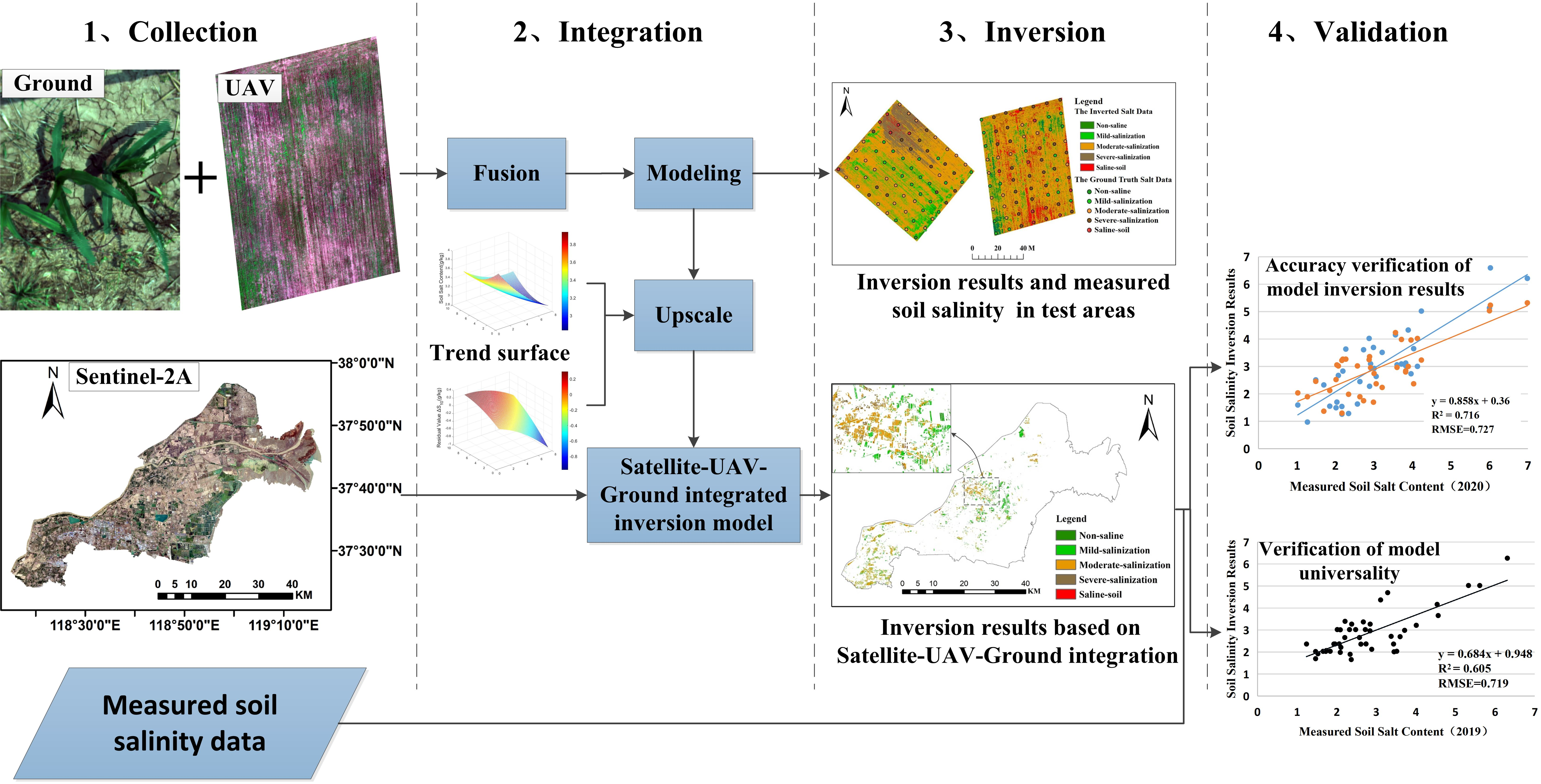
:Soil salinization is a significant factor affecting corn growth in coastal areas. How to use multi-source remote sensing data to achieve the target of rapid, efficient and accurate soil salinity monitoring in a large area is worth further study. In this research, using Kenli District of the Yellow River Delta as study area, the inversion of soil salinity in a corn planting area was carried out based on the integration of ground imaging hyperspectral, unmanned aerial vehicles (UAV) multispectral and Sentinel-2A satellite multispectral images. The UAV and ground images were fused, and the partial least squares inversion model was constructed by the fused UAV image. Then, inversion model was scaled up to the satellite by the TsHARP method, and finally, the accuracy of the satellite-UAV-ground inversion model and results was verified. The results show that the band fusion of UAV and ground images effectively enrich the spectral information of the UAV image. The accuracy of the inversion model constructed based on the fused UAV images was improved. The inversion results of soil salinity based on the integration of satellite-UAV-ground were highly consistent with the measured soil salinity (R2 = 0.716 and RMSE = 0.727), and the inversion model had excellent universal applicability. This research integrated the advantages of multi-source data to establish a unified satellite-UAV-ground model, which improved the ability of large-scale remote sensing data to finely indicate soil salinity.

1. Introduction
Globally, declining soil quality poses a significant challenge to improving agricultural productivity, economic growth and a healthy environment [1,2]. In coastal areas, soil salinity and alkalinity are major soil limiting factors for agricultural and land degradation [3]. Soil salinization not only reduces soil quality and land productivity, leading to a decline in crop yield, but also threatens ecological security and sustainable land use [4,5,6]. With the change of natural environment and the disturbance of human behavior, regional salinization becomes more and more serious, which affects the sustainable development of agriculture coastal areas to a great extent [7]. It is of great significance for agricultural production and sustainable development to accurately extract the soil salinization status and grasp its spatial distribution law in the main crop corn planting area of coastal areas.
To improve the accuracy and efficiency of obtaining regional soil salinization spatial distribution information is a prerequisite for rational management and utilization of salinized soil [8]. The traditional method of obtaining soil salinity information in the corn planting area is mainly through field survey sampling and laboratory testing, which is time consuming and laborious. Remote sensing technology has become a frequently used method for the quantitative analysis of soil salinization information because of its advantages of fast, large-scale, and non-destructive acquisition of ground feature information [9]. At present, ground, UAV and satellite remote sensing technologies provide a powerful means for monitoring the salt content of surface soils and have been widely used in the monitoring of farmland soil salinization [10,11,12,13]. Mohammad et al. [14] implemented the monitoring of soil salinity in a large area of Qom County, Qom Province, Iran, based on Sentinel-2A data. Wei et al. [15] took advantage of UAV equipped with Micro-MCA multispectral sensors to obtain images and realized the estimation of soil salinity in a small area of Hetao Irrigation District. Wang et al. [16] utilized a portable spectrometer ASD to obtain soil hyperspectral to construct a soil salinity inversion model in Baidunzi Basin, China, and achieved high model accuracy. However, most satellite images have low spatial resolution, so it is hard to achieve high precision real-time monitoring; UAV technology can obtain images with high temporal and spatial resolution, but the observation range is small, and it is unable to realize large scale monitoring; hyperspectral data can build high precision inversion models, but point information is incapable of monitoring soil salinity in a continuous spatial range. Therefore, due to the mutual constraints between the spatial resolution, spectral resolution and imaging width of the sensor, it is difficult for a single sensor to meet the requirements of large-scale, high precision and rapid soil salinity monitoring simultaneously [17]. Making full use of the complementary advantages of multi-source remote sensing data to carry out satellite-UAV-ground integrated inversion is an possible way to improve the accuracy of remote sensing inversion of regional soil salinity [18,19,20].
At present, Satellite-UAV-ground multi-source optical remote sensing data fusion has been applied to regional soil salinity inversion [21,22,23,24,25]. Solmaz et al. [26] constructed an inversion model through Landsat 8 and ASTER image fusion to obtain the spatial distribution of soil salinity in the Balikhli-Chay watershed, which improved the accuracy of soil salinity monitoring in the watershed. However, by the affection of inconsistency of sensor bands and satellite data acquisition time, the accuracy of soil salinity inversion after data fusion still needed to be improved. Zhang et al. [27] took advantage of band correction coefficients to normalize the reflectivity of satellite images based on the correlation between UAV and satellite image reflectivity, which improved the accuracy of soil salinity inversion, but the relationship between UAV and satellite image band spectrum information is nonlinear, and it was unable to accurately express the relationship between the two using only normalized coefficients. Sun et al. [28] used the measured soil hyperspectral data and Landsat-8 OLI multispectral data fusion to improve the retrieval accuracy of soil salt, and analyzed the differences of salt remote sensing in different seasons. Jia et al. [29] built a soil salinization estimation model based on the fusion of ASD hyperspectral and Landsat-8 OLI images, which expanded hyperspectral data from isolated point information to pixel and regional scale; however, due to the large spectral differences, it was difficult to effectively establish the corresponding relationship between the two samples, limiting the improvement of the inversion accuracy. In conclusion, the satellite-UAV-ground integration of regional soil salinity inversion is subject to the following limitations at present. First of all, the discrete hyperspectral observation data cannot accurately match the continuous spatial scale of UAV and satellite data; second, the simple linear method is used to fuse remote sensing data of different scales, and the accuracy of the inversion model built therefrom is limited; third, until now most of the inversion research based on satellite-UAV-ground multi-source remote sensing data fusion is based on the data fusion of two platforms, and the research of soil salinity inversion systems based on the integration of remote sensing data of three platforms still needs further exploration.
The overall objective of this research is to to explore the nonlinear fusion method of ground imaging hyperspectral and UAV multi-spectral images, build a soil salinity inversion model based on the fused UAV images, and then to try to construct a high accuracy inversion model based on satellite image through the upscaling method, so as to realize satellite-UAV-ground integrated soil salinity monitoring in a coastal corn planting area.
2. Materials and Methods
2.1. Study Area
The study area is located in Kenli District, which is located at the estuary of the Yellow River Delta, China (37°24′–38°10′N, 118°15′–119°19′E) (Figure 1). The area has a warm temperate continental monsoon climate with four distinct seasons [30]. The terrain in the area is typical of the delta landform, with a slight fan shape from southwest to northeast. The soil is developed on the alluvium of the Yellow River, with sandy loam in the majority; due to the lateral infiltration of the Yellow River and the jacking and impregnation of sea water, the land is irrigated backward, and the phenomenon of secondary salinization of the soil is more serious [31]. At present, there is still a large amount of unused saline-alkali wasteland, which has huge development and utilization potential. The main crops are winter wheat, corn, rice and cotton, with extensive management and low yield. Corn planting areas are mainly distributed in the southwest and in the middle, and the soil salinization variation is obvious, which is an ideal area for this research.
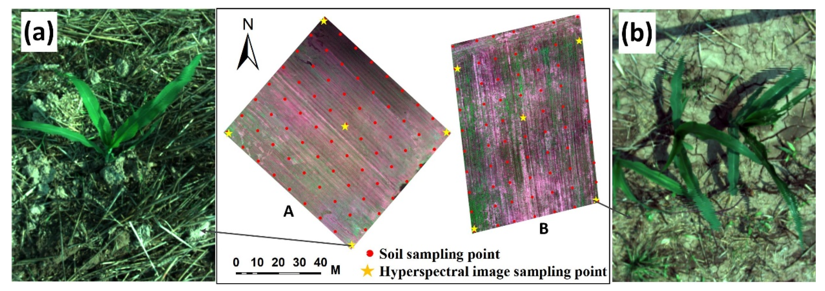
Based on the investigation of Kenli District, two test areas, A and B (Figure 1), were selected to carry out field measurement of soil salinity, ground imaging hyperspectral measurement and UAV flight test. Test area A was a rectangular area of 70 m× 80 m, and test area B was a rectangular area of 60 m × 90 m. Through investigation, the planting time, tillage methods, and fertilization conditions in the test areas A and B were basically the same, the growth of corn in the test areas was significantly different, and the soil salt content was distributed in all grades, which was typical and representative.
2.2. Data Acquisition and Processing
2.2.1. Ground Data Acquisition and Preprocessing
Field investigation in the study area was carried out on 14–15 July 2020, corn seedling stage. In order to ensure the uniform distribution of the points, 3 sample points were pre-arranged in every 5 km × 5 km grid in the study area, and finally 37 soil sample points in the corn planting area were collected for regional inversion verification. A ground card was placed every 10 m on the peripheral boundary of test area A and B respectively, and a 10 m× 10 m sample grid was formed after connecting with the measuring rope. Taking the grid intersection as the sampling point, a total of 142 sample points were collected, including 72 in test area A and 70 in test area B. The 6 outliers in the sampling points were eliminated, and the remaining 136 samples were used for the construction and verification of the corn soil salinity inversion model.
An EC110 portable salinity meter (Spectrum Technologies, Inc., Aurora, CO, USA) equipped with a 2225FST series probe (conductivity temperature correction had been completed) was used to measure the electrical conductivity of the soil surface 10 cm of the corn plant at each sample point, and the average value of multi-point measurement was taken as the EC value of each sample point, in dS/m. According to the previous research results of the laboratory, the formula SS = 2.18 × EC + 0.727 was applied to convert the measured EC data into the soil salt content (SS), in g/kg [32].
Hyperspectral images were obtained from a SOC710VP portable hyperspectral imager with a spectral range of 400–1000 nm, spectral resolution of 4.68 nm, 128 bands, and the lens type was C-Mount [33]. The hyperspectral image acquisition time was 11:00–15:00, the weather was clear and cloudless, and the wind was light. The SOC710VP was placed on a tripod, and the lens height was 1.6 m. Ten hyperspectral images were collected in the four corners and the center of the two test areas, as shown in Figure 2a,b. At the same time, the gray plate images were collected for correction. The ground range of the acquired images was 60 cm × 80 cm, and the images were processed to realize reflectance conversion.
2.2.2. UAV Data Collection and Preprocessing
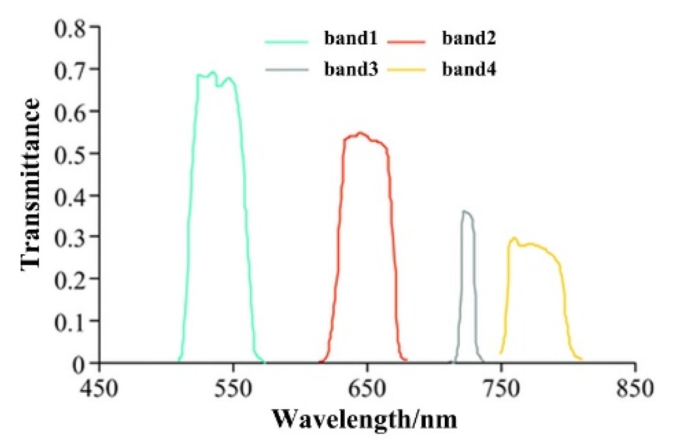
From 11:00–15:00 on 14–15 July 2020, the DJI Matrice 600 Pro six-rotor UAV (SZ DJI Technology Co., Ltd. Shenzhen, Guangdong Province, China) was equipped with a Sequoia multispectral camera (Parrot Sequoia, Parrot Inc., Paris, France) to obtain UAV images. The camera can receive a total of 4 bands of information, which are green light (G), red light (R), red edge (RE) and near infrared (NIR). Its spectral response function was shown in Figure 3. The Sequoia multi-spectral camera was fixed on the UAV gimbal, and the Sunshine sensor which measured the solar irradiance was mounted on the top of the UAV, and the radiation correction data were used to correct the image during the flight [34].
The Sequoia multispectral camera and radiation sensor were calibrated, and the ground standard whiteboard image was collected before the UAV took off. The flying height was 50 m, the flying speed was 5 m/s, and the image acquisition interval was 1.5 s. After the data were collected, they were imported into Pix4D Mapper software (Pix4D, Prilly, Switzerland) for splicing, radiation correction and other processing to obtain the high resolution ortho-reflection image of the test area, with a spatial resolution of 5 cm. In order to eliminate the random error caused by the reflectance of a single point, a 5 × 5 pixels-size image was taken with the sampling point as the center, and the average reflectance of the image was taken as the reflectance data of the sampling point.
2.2.3. Sentinel-2A Data Acquisition and Preprocessing
The Sentinel-2 satellite comprises two small satellites, A and B, with a revisit period of 5 days. The main payload is an MSI multispectral imager, covering the 0.4–2.4 μm spectral range, including 10 m (4 bands) and 20 m (6 bands), 60 m (3 bands) ground resolution [28]. The Sentinel-2A product was downloaded from the ESA Copernicus data sharing website (https://scihub.copernicus.eu/, accessed on 16 December 2020). Considering the acquisition time of ground and UAV data and the quality of the image, the Sentinel-2A Level-1C multispectral image on 15 July 2020 was selected for modeling and inversion of soil salinity, and images on 14 August 2020 and 18 October 2020 were selected for extraction of the corn planting areas.
Radiometric calibration, atmospheric correction and resampling of L1C data were carried out to generate images with a spatial resolution of 10 m, and the Sentinel-2A true color image of the study area was obtained by stitching and clipping (Figure 1). Four bands, B3, B4, B6 and B7, of Sentinel-2A image were selected which harmonized with the UAV image bands. The central wavelengths are 560 nm, 665 nm, 740 nm and 783 nm respectively, and the band widths are 45 nm, 38 nm, 18 nm and 28 nm respectively.
2.3. UAV-Ground Data Fusion
The mapping relationship between the coincidence area of the UAV and the ground image was established by utilizing the ground hyperspectrum and UAV pixel reflectivity of the homonymy points in the coincident area to solve the reconstruction of the spectral information of the non-coincident area. The fusion of high-fidelity space and spectral information of images with different widths was realized, so as to enrich the spectral information of the UAV image [35]. The spatial resolution of the ground hyperspectral image was resampled to 5 cm, which was the same as the spatial resolution of the UAV image. According to the spectral response function of the Sequoia sensor, the hyperspectral data were fitted into UAV band data by convolution operation. The calculation formula is shown in Equation (1) [36]:
where is the simulated UAV band reflectivity, is the UAV spectral response function, and are the upper and lower limits of the band, respectively, and is the ground hyperspectral data.
The relationship between ground hyperspectral and UAV image spectrum was non-linear [37], so the quadratic polynomial model was used to train the mapping relationship of the coincident area and expand the spectral information of the non-coincidence area, to realize the construction of a UAV image with rich spectral information and high spatial resolution. The quadratic polynomial model adopted is shown in Equation (2):
where a and b are spectral index conversion coefficients, c is the conversion residual, SU is the reflectance of unfused UAV image, and S′U is the reflectance of fused UAV image.
The reflectivity of pixels with homonymous points on the UAV and ground images were analyzed by fitting degree, and the consistency of spectral information between UAV band unfused and fused and the ground hyperspectrum was explored. The closer the fit degree was to 1, the higher the consistency between the two. The mathematical expression of the degree of fit (R2) is shown in Equation (3) [38]:
where is the reflectance of a certain point in the ground hyperspectrum, is the average reflectance of the sample points, and is the reflectance of the homonymous point in the UAV image. i = l, 2, …, n.
2.4. Construction of Soil Salinity Inversion Model Based on Fused UAV Images
2.4.1. Screening of UAV Image Vegetation Index
The vegetation index can show the characteristics of vegetation and effectively reflect the growth and health of vegetation [39]. When the degree of soil salinization becomes greater, the visible light reflectance of the vegetation increases, and the near-infrared reflectance decreases [40]. In this research, various vegetation indices related to red light and near-infrared were selected, mainly including normalized difference vegetation index (NDVI), normalized difference red edge index (NDRE), optimized soil adjusted vegetation index (OSAVI), difference vegetation index (DVI), normalized green difference vegetation index (GNDVI), and green-red vegetation index (GRVI).
The 6 vegetation indexes were calculated by the fused UAV band spectrum, and the formulas are shown in Table 1. The correlation coefficient between each vegetation index and soil salinity was calculated, and the variance inflation factor (VIF) between vegetation indexes was calculated by the formula VIF = 1/(1 − r × r) (r was the correlation coefficient between vegetation indexes) [41], excluding the low correlation or VIF > 10, which was the parameter that cannot be diagnosed by collinearity. The sensitive vegetation indexes were selected for soil salinity modeling.
2.4.2. Construction and Verification of Inversion Model
The salt contents of 136 samples were sorted from small to large, and the modeling set and validation set were sampled in a ratio of 2:1 to ensure that the construction model samples and the validation samples were evenly distributed. A total of 91 samples were selected for modeling and 45 samples were used for validation. Taking the sensitive vegetation indexes as the model input variable, the corn soil salinity inversion model was constructed by the PLS method [43], which was implemented in Matlab 2016B. The accuracy of model modeling and verification were evaluated by the coefficient of determination (R2) and root mean square error (RMSE). R2 measured the fitting degree of the model, and RMSE reflected the deviation between measured value and predicted value. The closer R2 was to 1, the smaller the RMSE, which means the higher the accuracy of the model, the better the effect.
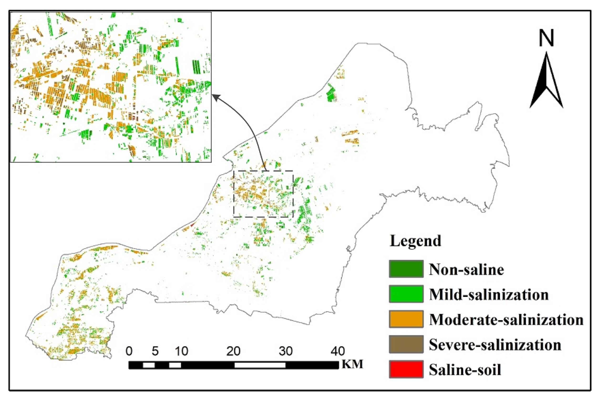
The degree of soil salinization is divided into 5 grades according to soil salinity and relevant criteria [44], non-salinization (<1 g/kg), mild salinization (1–2 g/kg), and moderate salinization (2–4 g/kg), severe salinization (4–6 g/kg) and saline soil (>6 g/kg), and the distribution map of soil salinity grade will be obtained.
2.5. Satellite-UAV Upscale Conversion of Soil Salinity Inversion Model
2.5.1. Information Extraction of the Corn Planting Area
The planting area of corn in the study area was extracted by the time series features composed of the NDVI of the Sentinel-2A images on 14 August 2020 and 18 October 2020. Based on the investigation and analysis of the vegetation types in the study area, the middle of August was the vigorous growth period of the vegetation, which was the best time to distinguish vegetation from non-vegetation, and October was the season when the corn had been harvested and the rice and cotton were mature, so the corn field was straw or bare land, showing lower NDVI vegetation characteristics. From August to October, the decrease in NDVI of corn crops was the largest, while the decrease in NDVI of other crops was less; the NDVI of forest and other green land remained basically unchanged. Therefore, through NDVI time series feature changes, combined with the training sample data, the following decision rules were established:
where NDVI8.14 was the NDVI image of Kenli District on 14 August 2020; NDVI10.18 was the NDVI image of 18 October 2020; and the corn planting area in the study area was obtained by masking.
2.5.2. Upscale Transformation of Inversion Model
The TsHARP method is often used for downscaling conversion of land surface temperature in remote sensing [45]. The method assumes that the relationship between surface temperature and NDVI remains unchanged at each scale, and the scale conversion of land surface temperature is realized by introducing NDVI to construct trend surface. This research improved the TsHARP method and introduced the PLS model constructed by NDVI, DVI and GRVI as the trend surface to achieve the upscaling conversion of the soil salinity inversion model.
Firstly, the relationship between soil salinity and trend surface factor at UAV scale was established:
S0.05 = F0.05 (B0.05)
S0.05—The soil salt content inverted by the trend surface transfer function at the UAV scale;
B0.05—Trend surface factors at the UAV scale, namely vegetation index NDVI, DVI and GRVI;
F0.05—Trend surface inversion function, which was also applicable to the inversion between soil salinity and trend surface factors upscaled to the 10 m spatial resolution of the Sentinel-2A satellite.
Considering that the trend surface may be affected by factors such as soil moisture content, it was difficult for the trend surface factor to fully reflect the distribution of soil salinity, which was reflected in the conversion residual ΔS0.05 on the UAV scale:
where S is the measured value of soil salinity.
ΔS0.05 = S − S0.05
Due to the error caused by the variation of soil spatial scale, the soil salt content S10 after scale conversion should be constituted of the soil salt content, which was calculated by applying the trend surface established on the UAV scale to the Sentinel-2A data, and ΔS10, which was the conversion residual of the UAV scale ΔS0.05 interpolated to the residual on the satellite scale. The calculation formula was S10 = F0.05 (B10) +ΔS10, and the satellite scale soil salinity inversion model was obtained.
2.5.3. Satellite-UAV-Ground Soil Salinity Inversion and Accuracy Verification
The satellite scale soil salinity inversion model was applied to Sentinel-2A image, and the distribution map of soil salinity in the corn planting area in Kenli District was obtained and compared with the measured values of soil salinity. At the same time, the results of satellite-UAV-ground integrated inversion were compared with the results of soil salinity inversion based on the PLS model built by the direct fusion of UAV and satellite. The R2 and RMSE of soil sampling points’ data and inversion results of two methods were calculated, respectively, and comparative analysis and quantitative evaluation were carried out.
In addition, in order to verify the universality of the model, the satellite-UAV-ground integrated inversion model was applied to the Sentinel-2A image of the Kenli corn planting area on 19 July 2019, and the spatial distribution of soil salinity was obtained. The measured soil salinity in the corn planting area and the inverted soil salinity were compared and verified.
3. Results and Analysis
3.1. Results of UAV-Ground Data Fusion
Table 2 presents the quadratic polynomial fusion model of four bands based on ground hyperspectral images and UAV multispectral images, as well as the fitting degree of the unfused and fused UAV image with the hyperspectral pixel of the homonymy points. The UAV and the hyperspectral bands have a high degree of fit, all greater than 0.6. The fitting degree of the four bands after fusion was significantly improved compared with unfusion, and the fitting degree of green, red, red-edge and near-red bands and hyperspectral bands were improved by 0.132, 0.096, 0.111 and 0.187, respectively. Therefore, the fusion of UAV and ground band can enrich the spectral information of the UAV image effectively.
3.2. Correlation between UAV Vegetation Index and Soil Salinity
Table 3 shows the correlation coefficient between vegetation index of fused UAV image and measured soil salinity. In the correlation coefficient matrix, vegetation index and soil salinity all had high correlation; the highest correlation coefficient between NDVI and soil salinity was 0.739, the lowest correlation coefficient between NDRE and soil salinity was 0.440. The VIF values of OSAVI, GNVI and DVI were all higher than 10, showing strong multicollinearity. Therefore, three vegetation indexes, NDVI, DVI and GRVI, were selected as the independent variables to construct the model.
3.3. The Soil Salinity Inversion Model Based on the UAV-ground Fusion Image and the Inversion Result of the Test Area
Table 4 illustrates the PLS model and its accuracy constructed by the three sensitive vegetation indexes of NDVI, DVI and GRVI before and after UAV fusion. The accuracy of the PLS inversion model based on the fused UAV images is better than the inversion model established without fusion. The R2 of the modeling set was improved by 0.104, and the RMSE was reduced by 0.22. The R2 of the verification set was improved by 0.109 and the RMSE decreased by 0.258. As a consequence, the inversion model based on the fused UAV images can improve the prediction ability of soil salinity.
For the salinity of the soil samples, the minimum value was 0.91 g/kg, the maximum value was 7.58 g/kg, and the average value was 4.48 g/kg. Soil samples covered all grades of soil salinization. Soil salinization is common in test areas A and B, and the salinity difference of samples is obvious.
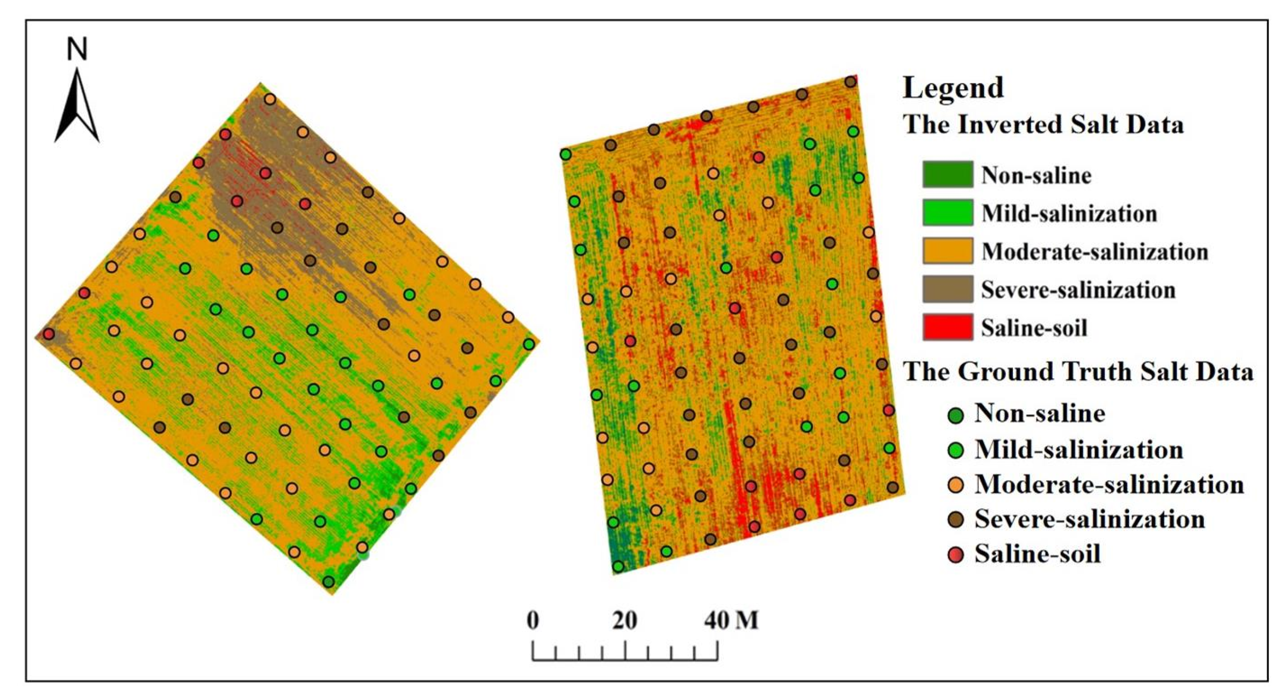
Figure 4 shows the spatial distribution of soil salinity in test areas A and B obtained by inversion of the PLS model constructed based on the fusion of UAV images. Among the 136 samples, the inverted values of 115 samples were consistent with the measured salinity grade on the ground, accounting for 84.5% of the total. The soil salinization in the two test areas were mainly light and moderate salinization, which was basically consistent with the field survey results in the test areas. The result indicates that the soil salinity inversion model based on the fused UAV data can obtain better inversion results and provide more powerful inversion ability.
3.4. Satellite-UAV-Ground Integrated Soil Salinity Upscale Inversion Model
3.4.1. Trend Surface Conversion Function
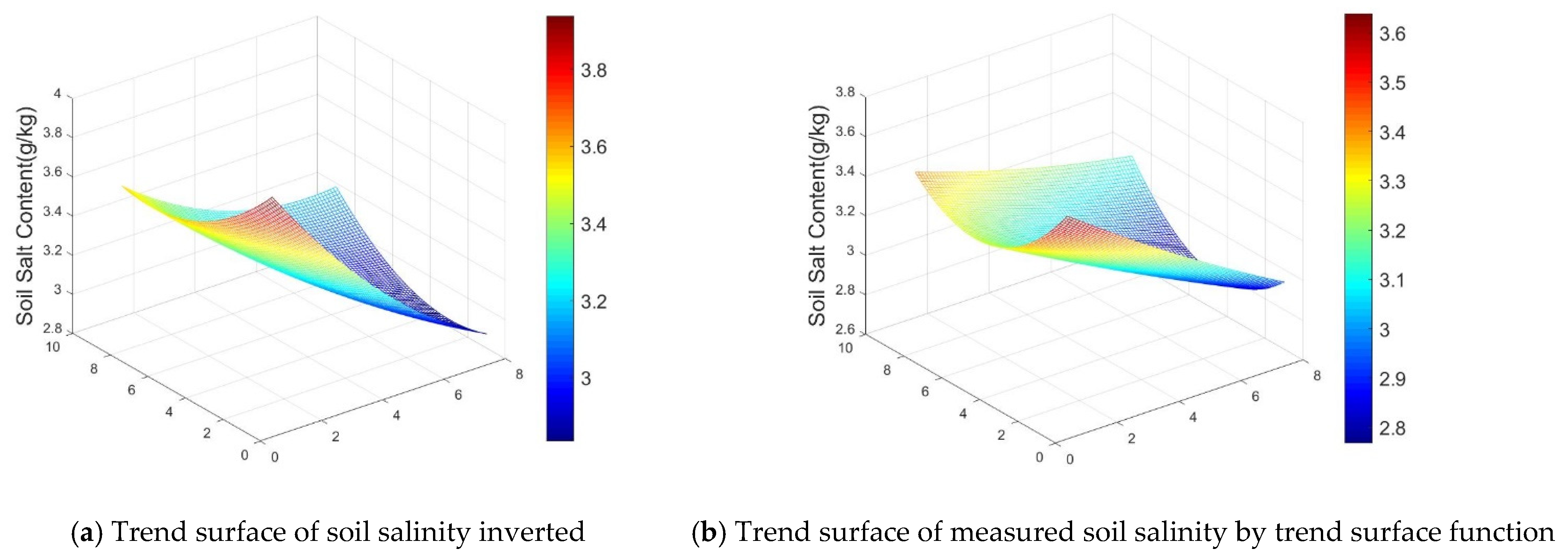
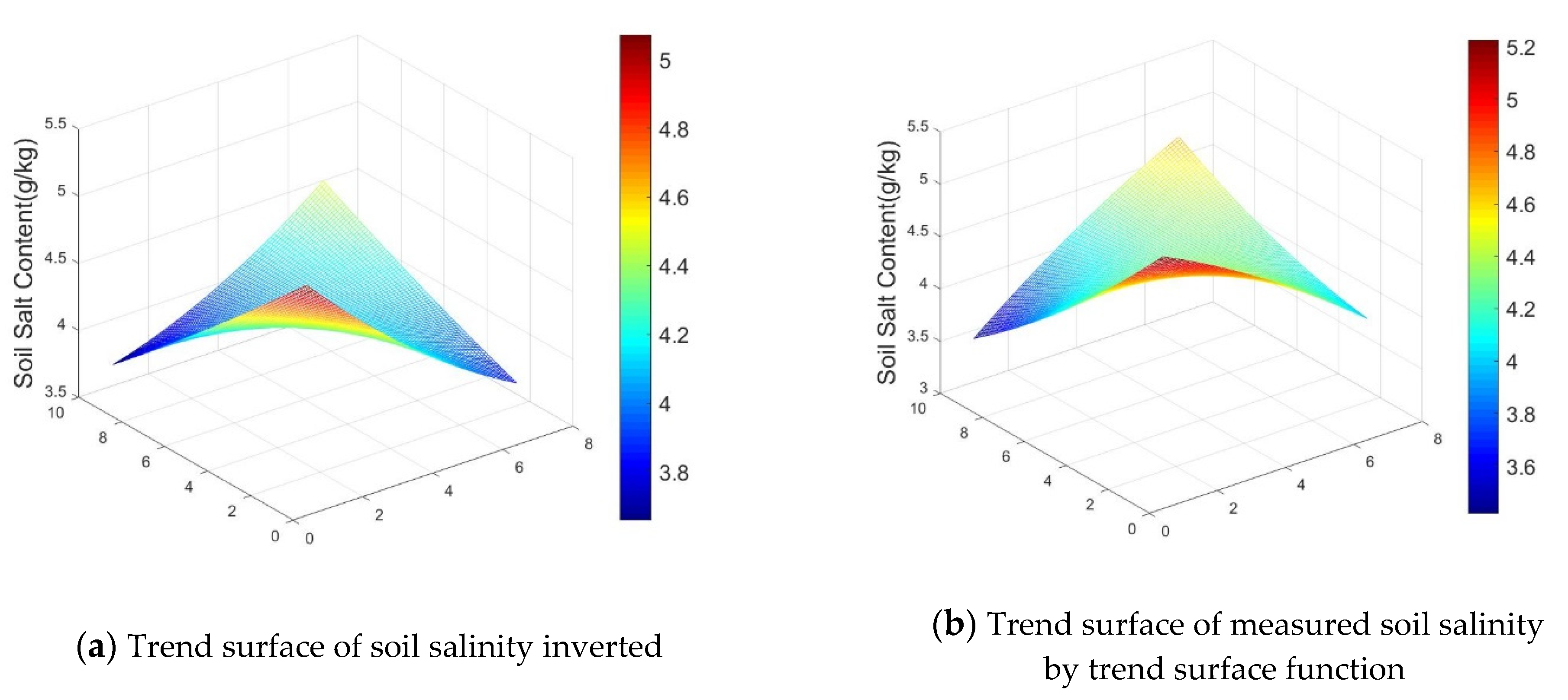
The PLS model based on the fused UAV images was used as the trend surface transformation function, that was F0.05 (B0.05) = 7.375–8.683 × NDVI − 3.083 × DVI + 0.211 × GRVI. Figure 5 and Figure 6 show the comparisons of the secondary trend surfaces of soil salinity obtained from the inversion of trend surface transfer functions and those measured. The results indicate that the spatial distribution trends of soil salinity in the two trend surfaces are basically the same; the trend surface transfer function can well reflect the spatial distribution trend of soil salinity in the study area.
3.4.2. Analysis of Upscale Residual Results
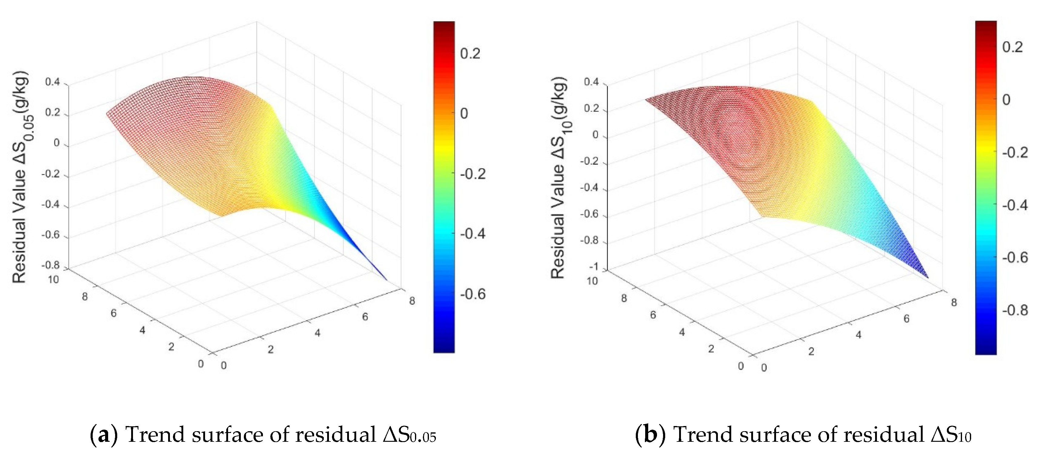
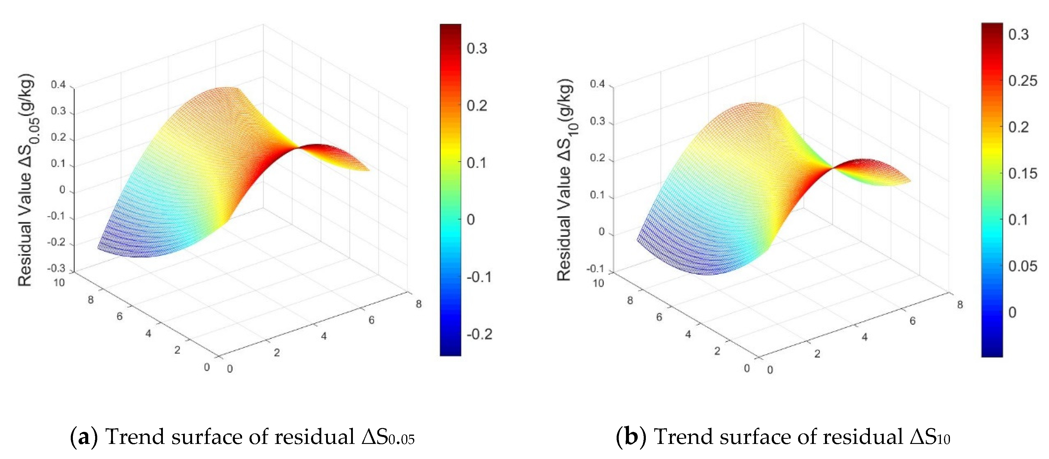
The UAV scale conversion residual ΔS0.05 was interpolated and converted to the satellite scale residual ΔS10. Table 5 shows the descriptive statistical features of residuals ΔS0.05 and ΔS10. There were some differences between residuals ΔS0.05 and ΔS10 of different scales. The maximum and standard deviations of ΔS10 were all less than ΔS0.05, and the minimum and average values were all larger than ΔS0.05; the distribution of ΔS10 was concentrated and the dispersion was low. Figure 7 and Figure 8 demonstrate secondary trend surfaces of test area A and B constructed by UAV residuals ΔS0.05 and Sentinel-2A residuals ΔS10, respectively. The spatial distribution structure of residual ΔS0.05 and ΔS10 trend surface was different, but the trend was basically the same.
Table 6 presents the correlation coefficients between residual ΔS10 and NDVI1, DVI1 and GRVI1 of Sentinel-2A images. The correlation coefficients were all over 0.6, indicating a high correlation. The PLS model established by the above three vegetation indexes and the residual ΔS10 was ΔS10 = −1.161 + 2.347 × NDVI1 − 4.505 × DVI1 − 0.08 × GRVI1.
3.4.3. Satellite-UAV-Ground Integrated Inversion Model
The trend surface transfer function was applied to the inversion of soil salinity at sentinel-2A satellite scale, and F0.05 (B10) = 7.375–8.683 × NDVI1 − 3.083 × DVI1 + 0.211 × GRVI1 was obtained. According to the above residual analysis results, the PLS model of the satellite scale residual ΔS10 was ΔS10 = −1.161 + 2.347 × NDVI1 − 4.505 × DVI1 − 0.08 × GRVI1. Therefore, the satellite scale PLS inversion model of soil salinity was S10 = F0. 05 (B10) + ΔS10 = 6.214–6.336 × NDVI1 − 7.588 × DVI1 + 0.131 × GRVI1; thus, the satellite-UAV-ground integrated soil salinity inversion model was obtained.
3.5. Corn Planting Area and Analysis of the Results of Soil Salinity Inversion
Figure 9 shows the corn planting area extracted by NDVI time series and decision rules. The different colors indicate the inversion results of soil salinity in the corn planting area obtained by using the satellite-UAV-ground integrated inversion model. Table 7 illustrates the area statistics of different soil salinity grades. The result shows that soil salinization was common in the whole corn planting area. The non-salinized soil was less distributed; most areas were mild salinized and moderate salinized soil, accounting for 88.36% of the total area, which are mainly distributed in the relatively high topography of the southwest and central regions. The area of severe salinized and saline soil was small, and it was scattered in the corn planting area. The inversion result was consistent with the actual survey situation in the study area and the distribution trend of soil salinity previously studied [22,28], indicating the validity of the model for accurate inversion of soil salinity.
3.6. Verification of the Accuracy of the Inversion Model
3.6.1. Accuracy Verification of Model Inversion Results
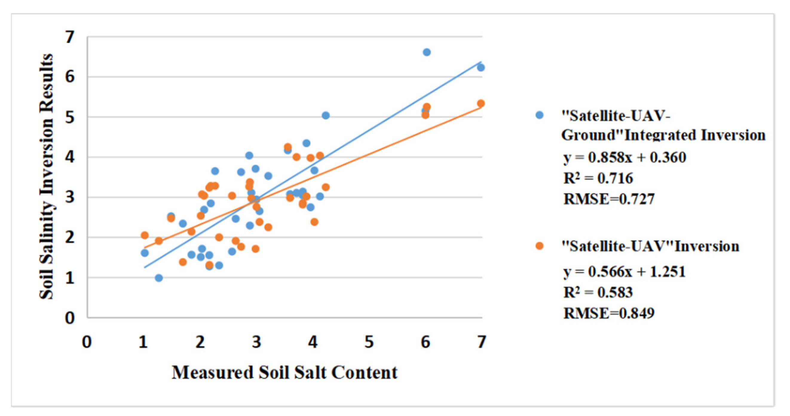
The soil salinity obtained from the satellite-UAV-ground integrated inversion and the satellite-UAV inversion at 37 sampling sites in the Kenli corn planting area were compared with the measured soil salinity to establish the scatter plot—the result is shown in Figure 10. The R2 and RMSE of the satellite-UAV-ground integrated inversion and the measured value were 0.716 and 0.727, respectively, suggesting the inversion results and the measured value were high consistency. Compared with the satellite-UAV inversion, the value of R2 was higher by 0.133 and the value of RMSE was lower by 0.122. Therefore, the consistency between the results of the satellite-UAV-ground integrated inversion and the measured data was higher than that of the satellite-UAV inversion, and the satellite-UAV-ground integrated inversion model had a better accuracy for the large-scale soil salinity inversion.
3.6.2. Verification of Model Universality
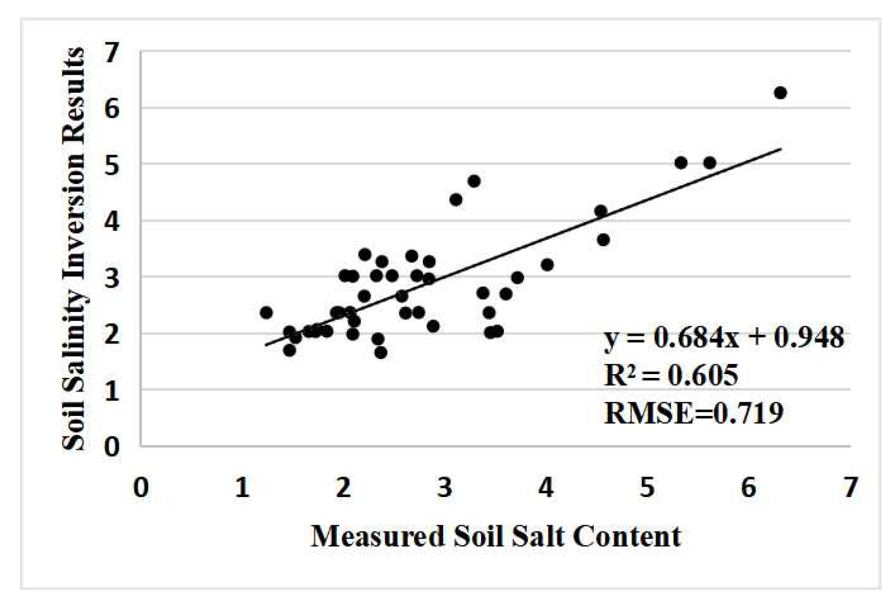
The Sentinel-2A image of the corn planting area on 19 July 2019 and the measured soil salt content at 44 ground points were used to verify the universality of the inversion model of corn soil salinity. Figure 11 is a scatter plot of the inversion results of soil salinity in the corn planting area and the measured soil salinity. The result was R2 = 0.605, RMSE = 0.719, indicating that the inversion result had good coherence to the measured soil salinity, and the model could be used as an inversion model of soil salinity in corn seedlings in coastal areas.
4. Discussion
(1) In coastal soil salinization areas, soil salinity is the main factor affecting the growth of corn and other crops, and other factors such as soil texture, fertility and nutrients, and soil moisture have relatively balanced effects on crop growth. Therefore, the difference of vegetation indexes only considers the influence of soil salinity, and the soil salinity is indirectly inverted through the vegetation index, which has been confirmed by previous studies [46,47,48,49]. The relationship between vegetation index and soil salinity of crops under different environmental conditions and at different times is distinct, so the established satellite-UAV-ground integrated inversion model is more suitable for the inversion of soil salinity in the corn seedling stage in coastal areas. The model was used to invert corn soil salinity at the seedling stage in 2019, and the results confirmed the universal applicability of the model.
(2) Francos et al. found that the traditional field non-imaging spectral data are discrete and easily affected by the soil background [50], while the ground hyperspectral imaging technology has the characteristics of image and spectrum integration, which can accurately determine the spectral information of the corn at the sampling point. The fusion of spectral information of ground hyperspectral and UAV image effectively improves the ability of UAV images to accurately express corn spectral information. Therefore, the accuracy of the soil salt inversion model which was constructed by UAV images fused with hyperspectral imaging data has been significantly improved.
(3) The four bands of the UAV image were fused with the ground hyperspectral image, and the degree of fitting was improved. However, the highest degree of fitting was 0.801, which was still different from the spectral information of the ground hyperspectral image. This is consistent with the results of previous studies [51,52]. Firstly, the divergence, probably due to the quadratic polynomial model used in image fusion, fails to fully explore the internal relationship between the data. The second possibility is the uncertainty of remote sensing data, and the band response functions of different sensors are different. When spectral response function is used for UAV band spectral matching, spectral information will be lost. Therefore, the next step of research should adopt more effective deep-level and high-level feature mining methods, such as deep learning methods [53], and improve the matching accuracy of the spectrum and space of the image to be fused to reduce the influence of radiation and spatial characteristics on the fusion accuracy. The data fusion method in this research has conducted a preliminary study on the fusion of images of different widths and provided a reference for ideas and methodology.
(4) The focus of this research was the exploration of the integration method of satellite, UAV and ground. Therefore, only the PLS inversion model was constructed. By the foundation of the effectiveness of integrated satellite-UAV-ground inversion in this research, the next step will be to integrate multi-dimensional features such as spectral features, spatial textures, and crop parameters to construct higher-precision models such as machine learning [54,55], and to screen the optimal model to further improve the accuracy of the regional soil salinity inversion.
(5) The heterogeneity of the surface space seriously affects the spatial scale conversion. The trend surface analysis method uses the multivariate statistical method to fit the distribution of spatial elements. In this research, the trend surface was used to simulate the spatial change trend of soil salinity, and the residual surface was used to simulate and quantify the spatial variability of the residual. As the scale increases, the variability of the soil salt residual becomes weaker and the standard deviation decreases; this agrees with the multi-scale variation law of soil salinity in the study area [56]. The influence of information loss and variation in the process of spatial scale upscaling is unavoidable [57,58]. The formulation description of scale transformation and the construction of a better continuous model are worthy of exploration.
(6) The satellite-UAV-ground integrated approach proposed in this study improves the monitoring accuracy of regional soil salinization. Compared with the previous satellite-UAV upscale inversion method, the inversion quality of the satellite-UAV-ground integration was better [59,60,61]. Although satellite-UAV upscaling improves the spatial resolution of satellite images, the improvement of inversion accuracy was still limited by the restriction of spectral information. Compared with the traditional scaling up method, the spectral information of the original remote sensing data can be improved, and the spatial structure characteristics can be maintained by introducing the high-resolution spectral information fusion and constructing the trend surface to realize the ascending scale conversion. The integrated satellite-UAV-ground method proposed in this research can be used for large-scale inversion of other surface parameters for reference.
5. Conclusions
In this research, ground-based hyperspectral imaging and UAV were fused to construct an inversion model of corn soil salinity, and the model was scaled up to Sentinel-2A satellite scale; the satellite-UAV-ground integrated inversion of soil salinity in the coastal corn planting area was realized. The main conclusions are as follows:
- (1)
- The fusion of the four bands of the UAV image with the ground hyperspectral improved the degree of fitting with the hyperspectral data. The vegetation indexes based on the UAV band after fusion had a high correlation with soil salinity. According to the correlation coefficient and variance expansion factor, three sensitive vegetation indexes, NDVI, DVI, and GRVI, were selected as independent variables for PLS modeling and R2 = 0.743; thus, the inversion results were coincident with the actual distribution of soil salinity in the test area.
- (2)
- The PLS model S0.05 = 7.375–8.683 × NDVI − 3.083 × DVI + 0.211 × GRVI constructed with the fused UAV images was used as the trend surface conversion function, and the PLS model of the residual ΔS10 was constructed as ΔS10 = −1.161 + 2.347 × NDVI1 − 4.505 × DVI1 − 0.08 × GRVI1. Thus, the Sentinel-2A satellite scale PLS inversion model of soil salinity in the coastal corn planting area of S10 = 6.214–6.336 × NDVI1 − 7.588 × DVI1 + 0.131 × GRVI1 was obtained.
- (3)
- The actual soil salinity in the corn planting area was used to verify the inversion results of satellite-UAV-ground integration and satellite-UAV ascending scale, and the inversion results of satellite-UAV-ground were better than those of satellite-UAV inversion and had high consistency with the actual salt distribution. The Sentinel-2A image of corn growing area on 19 July 2019 was used to verify the universality of the model; the R2 of soil salt inversion and measured soil salt was 0.605, which indicated that the model had an excellent universality.
- (4)
- The distribution of non-salinized soil in the study area was small, and the majority was mild and moderate salinized soil, accounting for 88.36% of the total area, which was concentrated in the southwest and central part of Kenli District, while the distribution of severe salinized soil and salinized soil was small and scattered in the corn planting area.
In this research, we proposed a satellite-UAV-ground integrated soil salinity inversion method in the coastal corn planting area, which provides an effective means for quickly and accurately obtaining soil salinity information in the corn area.
Author Contributions
Conceptualization, G.Q. and G.Z.; methodology, G.Q. and G.Z.; software, P.G.; validation, C.C.; formal analysis, G.Q.; investigation, P.G.; resources, W.Y.; data curation, G.Q. and W.Y.; writing—original draft preparation, G.Q.; writing—review and editing, G.Z. and C.C.; visualization, W.Y.; supervision, P.G.; project administration, C.C.; funding acquisition, W.Y. and G.Z. All authors have read and agreed to the published version of the manuscript.
Funding
This research was funded by National Natural Science Foundation of China (No. 41877003), Major Science and Technology Innovation Project of Shandong Province (No. 2019JZZY010724), Shandong Province “Double First-Class” Award and Subsidy Fund (No. SYL2017XTTD02), Talent Startup Project of Zhejiang A& F University (No. 113-2034020162).
Institutional Review Board Statement
Not applicable.
Informed Consent Statement
Not applicable.
Data Availability Statement
Not applicable.
Conflicts of Interest
The authors declare no conflict of interest.
References
- Hassan, F.; Mohammad, A.; Brandon, H.; Hamid, S.; Asghar, R.; Abolhasan, F.; Thomas, S.; Ruhollah, T. Spatio-temporal dynamic of soil quality in the central Iranian desert modeled with machine learning and digital soil assessment techniques. Ecol. Indic. 2020, 118, 106736. [Google Scholar] [CrossRef]
- Abedi, F.; Amirian-Chakan, A.R.; Faraji, M.; Taghizadeh-Mehrjardi, R.; Kerry, R.; Razmjoue, D.; Scholten, T. Salt dome induced soil salinity in southern Iran–prediction and mapping with averaging machine learning models. Land Degrand. Dev. 2020, 32, 1540–1554. [Google Scholar] [CrossRef]
- Girmay, G.; Singh, B.; Mitiku, H.; Borresen, T.; Lal, R. Carbon stocks in Ethiopian soils in relation to land use and soil management. Land Degrand. Dev. 2008, 19, 351–367. [Google Scholar] [CrossRef]
- Metternicht, G.I.; Zinck, J.A. Remote sensing of soil salinity: Potentials and constraints. Remote Sens. Environ. 2003, 85, 1–20. [Google Scholar] [CrossRef]
- Allbed, A.; Kumar, L.; Aldakheel, Y.Y. Assessing soil salinity using soil salinity and vegetation indices derived from IKONOS high-spatial resolution imageries: Applications in a date palm dominated region. Geoderma 2014, 230, 1–8. [Google Scholar] [CrossRef]
- Xu, X.; Zhao, G.X.; Gao, P.; Cui, K.; Li, T. Inversion of Soil Salinity in Coastal Winter Wheat Growing Area Based on Sentinel Satellite and Unmanned Aerial Vehicle Multi-Spectrum—A Case Study in Kenli District of the Yellow River Delta. Sci. Agric. Sin. 2020, 53, 5005–5016. [Google Scholar]
- Maleki, S.; Karimi, A.; Zeraatpisheh, M.; Poozeshi, R.; Feizi, H. Long-term cultivation effects on soil properties variations in different landforms in an arid region of eastern Iran. Catena 2021, 206, 105465. [Google Scholar] [CrossRef]
- Abbas, A.; Khan, S.; Hussain, N.; Hanjra, M.A.; Akbar, S. Characterizing soil salinity in irrigated agriculture using a remote sensing approach. Phys. Chem. Earth 2013, 55, 43–52. [Google Scholar] [CrossRef]
- Wang, Z.; Zhang, X.; Zhang, F.; Chan, N.; Kung, H.; Liu, S.; Deng, L. Estimation of soil salt content using machine learning techniques based on remote-sensing fractional derivatives, a case study in the Ebinur Lake Wetland National Nature Reserve, Northwest China. Ecol. Indic. 2020, 119, 106869. [Google Scholar] [CrossRef]
- Aldabaa, A.; Weindorf, D.C.; Chakraborty, S.; Sharma, A.; Li, B. Combination of proximal and remote sensing methods for rapid soil salinity quantification. Geoderma 2015, 239, 34–46. [Google Scholar] [CrossRef] [Green Version]
- El Harti, A.; Lhissou, R.; Chokmani, K.; Ouzemou, J.E.; Hassouna, M.; Bachaoui, E.M.; El Ghmari, A. Spatiotemporal monitoring of soil salinization in irrigated Tadla Plain (Morocco) using satellite spectral indices. Int. J. Appl. Earth Obs. 2016, 50, 64–73. [Google Scholar] [CrossRef]
- Zhang, T.T.; Qi, J.G.; Gao, Y.; Ouyang, Z.T.; Zeng, S.L.; Zhao, B. Detecting soil salinity with MODIS time series VI data. Ecol. Indic. 2015, 52, 480–489. [Google Scholar] [CrossRef]
- Nurmemet, I.; Ghulam, A.; Tiyip, T.; Elkadiri, R.; Ding, J.L.; Maimaitiyiming, M.; Abliz, A.; Sawut, M.; Zhang, F.; Abliz, A.; et al. Monitoring Soil Salinization in Keriya River Basin, Northwestern China Using Passive Reflective and Active Microwave Remote Sensing Data. Remote Sens. 2015, 7, 8803–8829. [Google Scholar] [CrossRef] [Green Version]
- Mohammad, M.T.; Mahdi, H.; Kamran, E. Retrieval of soil salinity from Sentinel-2 multispectral imagery. Eur. J. Remote Sens. 2019, 52, 138–154. [Google Scholar]
- Wei, G.; Li, Y.; Zhang, Z.; Chen, Y.; Chen, J.; Yao, Z.; Lao, C.; Chen, H. Estimation of soil salt content by combining UAV-borne multispectral sensor and machine learning algorithms. PeerJ 2020, 8, e9087. [Google Scholar] [CrossRef] [PubMed]
- Wang, L.; Zhang, B.; Shen, Q.; Yao, Y.; Zhang, S.; Wei, H.; Yao, R.; Zhang, Y. Estimation of Soil Salt and Ion Contents Based on Hyperspectral Remote Sensing Data: A Case Study of Baidunzi Basin, China. Water 2021, 13, 559. [Google Scholar] [CrossRef]
- Berra, E.F.; Gaulton, R.; Barr, S. Assessing spring phenology of a temperate woodland: A multiscale comparison of ground, unmanned aerial vehicle and Landsat satellite observations. Remote Sens. Environ. 2019, 223, 229–242. [Google Scholar] [CrossRef]
- Liu, X.; Liu, Q.; Wang, Y.J. Remote sensing image fusion based on two-stream fusion network. Inform. Fusion 2020, 55, 1–5. [Google Scholar] [CrossRef] [Green Version]
- Wu, W.; Al-Shafie, W.M.; Mhaimeed, A.S.; Ziadat, F.; Nangia, V.; Payne, W.B. Soil salinity mapping by multiscale remote sensing in mesopotamia, Iraq. IEEE J. Sel. Top. Appl. Earth Obs. Remote Sens. 2017, 7, 4442–4452. [Google Scholar] [CrossRef]
- He, C.Y.; Gao, B.; Huang, Q.X.; Ma, Q.; Dou, Y.Y. Environmental degradation in the urban areas of China: Evidence from multi-source remote sensing data. Remote Sens. Environ. 2017, 193, 65–75. [Google Scholar] [CrossRef]
- Xu, C.; Qu, J.J.; Hao, X.; Cosh, M.H.; Prueger, J.H.; Zhu, Z.; Gutenberg, L. Downscaling of surface soil moisture retrieval by combining MODIS/Landsat and in situ measurements. Remote Sens. 2018, 10, 210. [Google Scholar] [CrossRef] [Green Version]
- Ma, Y.; Chen, H.; Zhao, G.X.; Wang, Z.R.; Wang, D.Y. Spectral Index Fusion for Salinized Soil Salinity Inversion Using Sentinel-2A and UAV Images in a Coastal Area. IEEE Access 2020, 8, 159595–159608. [Google Scholar] [CrossRef]
- Kattenborn, T.; Lopatin, J.; Förster, M.; Braun, A.C.; Fassnacht, F.E. UAV data as alternative to field sampling to map woody invasive species based on combined Sentinel-1 and Sentinel-2 data. Remote Sens. Environ. 2019, 227, 61–73. [Google Scholar] [CrossRef]
- Kattenborn, T.; Eichel, J.; Fassnacht, F.E. Convolutional Neural Networks enable efficient, accurate and fine-grained segmentation of plant species and communities from high-resolution UAV imagery. Sci. Rep. 2019, 9, 9–23. [Google Scholar] [CrossRef] [PubMed]
- Guo, Y.; Shi, Z.; Huang, J.Y.; Zhou, L.Q.; Zhou, Y.; Wang, L. Characterization of field scale soil variability using remotely and proximally sensed data and response surface method. Stoch. Environ. Res. Risk Assess. 2016, 30, 859–869. [Google Scholar] [CrossRef]
- Fathololoumi, S.; Vaezi, A.R.; Alavipanah, S.K.; Ghorbani, A.; Saurette, D.; Biswas, A. Improved digital soil mapping with multitemporal remotely sensed satellite data fusion: A case study in Iran. Sci. Total Environ. 2020, 721, 137703. [Google Scholar] [CrossRef] [PubMed]
- Zhang, S.M.; Zhao, G.X. A Harmonious Satellite-Unmanned Aerial Vehicle-Ground Measurement Inversion Method for Monitoring Salinity in Coastal Saline Soil. Remote Sens. 2019, 11, 1700. [Google Scholar] [CrossRef] [Green Version]
- Sun, Y.N.; Li, X.Y.; Shi, H.B.; Cui, J.Q.; Wang, W.G.; Bu, X.Y. Remote Sensing Inversion of Soil Salinity and Seasonal Difference Analysis Based on Multi-source Data Fusion. Trans. Chin. Soc. Agric. Mach. 2020, 51, 169–180. [Google Scholar]
- Jia, P.P.; Sun, Y.; Shang, T.H.; Zhang, J.H. Estimation models of soil water-salt based on hyperspectral and Landsat-8 OLI image. Chin. J. Ecol. 2020, 39, 2456–2466. [Google Scholar]
- Zhao, Q.Q.; Bai, J.H.; Gao, Y.C.; Zhao, H.X.; Zhang, G.L.; Cui, B.S. Shifts in the soil bacterial community along a salinity gradient in the Yellow River Delta. Land Degrad. Dev. 2020, 31, 2255–2267. [Google Scholar] [CrossRef]
- Wen, Y.; Guo, B.; Zang, W.Q.; Ge, D.Z.; Luo, W.; Zhao, H.H. Desertification detection model in Naiman Banner based on the albedo-modified soil adjusted vegetation index feature space using the Landsat8 OLI images. Geomat. Nat. Hazards Risk 2019, 10, 544–558. [Google Scholar] [CrossRef]
- Wang, Z.R.; Zhao, G.X.; Gao, M.X.; Chang, C.Y.; Jiang, S.Q.; Jia, J.C.; Li, J. Spatial variability of soil water and salt in summer and soil salt microdomain characteristics in Kenli County, Yellow River Delta. Acta Ecol. Sin. 2016, 36, 1040–1049. [Google Scholar]
- Wen, X.; Zhu, X.C.; Yu, R.Y.; Xiong, J.L.; Gao, D.S.; Jiang, Y.M.; Yang, G.J. Visualization of Chlorophyll Content Distribution in Apple Leaves Based on Hyperspectral Imaging Technology. Agric. Sci. China 2019, 10, 783–795. [Google Scholar] [CrossRef] [Green Version]
- Dong, C.; Zhao, G.X.; Su, B.W.; Chen, X.N.; Zhang, S.M. Research on the Decision Model of Variable Nitrogen Application in Winter Wheat’s Greening Period Based on UAV Multispectral Image. Spectrosc. Spect. Anal. 2019, 39, 3599–3605. [Google Scholar]
- He, J.; Li, J.; Yuan, Q.Q.; Li, H.F.; Shen, H.F. Spatial–Spectral Fusion in Different Swath Widths by a Recurrent Expanding Residual Convolutional Neural Network. Remote Sens. 2019, 11, 2203. [Google Scholar] [CrossRef] [Green Version]
- Zhang, F.; Tashpolat, T.; Ding, J.L. Simulation and Subsection between Fields Measured Endmember Spectrum and Multi-spectrum Image of TM. Opto-Electron. Eng. 2012, 39, 62–70. [Google Scholar]
- Shao, Z.; Cai, J. Remote sensing image fusion with deep convolutional neural network. IEEE J. Sel. Top. Appl. Earth Obs. Remote Sens. 2018, 11, 1656–1669. [Google Scholar] [CrossRef]
- Said, N.; Henning, B.; Joachim, H. Digital Mapping of Soil Properties Using Multivariate Statistical Analysis and ASTER Data in an Arid Region. Remote Sens. 2015, 7, 1181–1205. [Google Scholar]
- Wang, X.; Zhang, F.; Ding, J.; Latif, A. Johnson VC. Estimation of soil salt content (SSC) in the Ebinur Lake Wetland National Nature Reserve (ELWNNR), Northwest China, based on a Bootstrap-BP neural network model and optimal spectral indices. Sci. Total Environ. 2018, 615, 918–930. [Google Scholar] [CrossRef] [PubMed]
- Tilley, D.R.; Ahmed, M.; Son, J.H.; Badrinarayanan, H. Hyperspectral Reflectance Response of Freshwater Macrophytes to Salinity in a Brackish Subtropical Marsh. J. Environ. Qual. 2007, 36, 780–789. [Google Scholar] [CrossRef] [PubMed]
- Chen, H.Y.; Zhao, G.X.; Chen, J.C.; Wang, R.Y.; Gao, M.X. Remote sensing inversion of saline soil salinity in the mouth of the Yellow River based on improved vegetation index. Trans. Chin. Soc. Agric. Eng. 2015, 31, 107–114. [Google Scholar]
- Dong, J.J.; Niu, J.M.; Zhang, Q.; KangSa, R.L.; Han, F. Remote sensing yield estimation of typical grassland based on multi-source satellite data. Chin. J. Grassl. 2013, 35, 64–69. [Google Scholar]
- Xu, L.; Wang, Q. Retrieval of soil water content in saline soils from emitted thermal infrared spectra using partial linear squares regression. Remote Sens. 2015, 7, 14646–14662. [Google Scholar] [CrossRef] [Green Version]
- Bao, S.D. Soil Agrochemical Analysis; China Agriculture Press: Beijing, China, 2000. [Google Scholar]
- Li, X.J.; Xin, X.Z.; Jiang, T. Spatial downscaling research of satellite land surface temperature based on spectral normalization index. Acta Geod. Cartogr. Sin. 2017, 46, 353–361. [Google Scholar]
- Wu, W.C. The Generalized Difference Vegetation Index (GDVI) for Dryland Characterization. Remote Sens. 2014, 6, 1211–1233. [Google Scholar] [CrossRef] [Green Version]
- Scudiero, E.; Skaggs, T.H.; Corwin, D.L. Regional-scale soil salinity assessment using Landsat ETM + canopy reflectance. Remote Sens. Environ. 2015, 169, 335–343. [Google Scholar] [CrossRef] [Green Version]
- Fernández-Buces, N.; Siebe, C.; Cram, S.; Palacio, J.L. Mapping soil salinity using a combined spectral response index for bare soil and vegetation: A case study in the former lake Texcoco, Mexico. J. Arid. Environ. 2006, 65, 644–667. [Google Scholar] [CrossRef]
- Qi, G.H.; Zhao, G.X.; Xi, X. Soil salinity inversion of winter wheat areas based on satellite-unmanned aerial vehicle-ground collaborative system in coastal of the Yellow River Delta. Sensors 2020, 20, 6521. [Google Scholar] [CrossRef] [PubMed]
- Francos, N.; Romano, N.; Nasta, P.; Zeng, Y.; Szabó, B.; Manfreda, S.; Ciraolo, G.; Mészáros, J.; Zhuang, R.; Su, B.; et al. Mapping Water Infiltration Rate Using Ground and UAV Hyperspectral Data: A Case Study of Alento, Italy. Remote Sens. 2021, 13, 2606–2636. [Google Scholar] [CrossRef]
- Youme, O.; Bayet, T.; Dembele, J.; Cambier, C. Deep Learning and Remote Sensing: Detection of Dumping Waste Using UAV. Procedia Comput. Sci. 2021, 185, 361–369. [Google Scholar] [CrossRef]
- Azarang, A.; Kehtarnavaz, N. Image fusion in remote sensing by multi-objective deep learning. Int. J. Remote Sen. 2020, 41, 9507–9524. [Google Scholar] [CrossRef]
- Chen, L.; Liu, C.; Chang, F.; Li, S.; Nie, Z. Adaptive multi-level feature fusion and attention-based network for arbitrary-oriented object detection in remote sensing imagery. Neurocomputing 2021, 451, 67–80. [Google Scholar] [CrossRef]
- Wang, J.; Huang, B.; Zhang, H.; Ma, P. Sentinel-2A Image Fusion Using a Machine Learning Approach. IEEE Geosci. Remote 2019, 57, 9589–9601. [Google Scholar] [CrossRef]
- Li, J.; Guo, X.; Lu, G.; Zhang, B.; Xu, Y.; Wu, F.; Zhang, D. DRPL: Deep Regression Pair Learning For Multi-Focus Image Fusion. IEEE Trans Image Process 2020, 29, 4816–4831. [Google Scholar] [CrossRef]
- Edoardo, A.C.; Costantini, G. Beyond the concept of dominant soil: Preserving pedodiversity in upscaling soil maps. Geoderma 2016, 271, 243–253. [Google Scholar] [CrossRef]
- Zhang, X.; Zuo, W.; Zhao, S.; Jiang, L.; Chen, L.; Zhu, Y. Uncertainty in Upscaling In Situ Soil Moisture Observations to Multiscale Pixel Estimations with Kriging at the Field Level. ISPRS In. J. Geo-Inf. 2018, 7, 33. [Google Scholar] [CrossRef] [Green Version]
- Cui, K.; Zhao, G.X.; Wang, Z.R.; Xi, X.; Gao, P.P.; Qi, G.H. Multi-scale spatial variability of soil salinity in typical fields of the Yellow River Delta in summer. Chin. J. Appl. Ecol. 2020, 31, 1451–1458. [Google Scholar]
- Hu, J. Estimation of Soil Salinity in Arid Area Based on Multi-Source Remote Sensing. Master’s Thesis, Zhejiang University, Hangzhou, China, 2019. [Google Scholar]
- Chen, W.J. Soil Salinity Retrieval and Dynamic Analysis Based Onspectral Intercalibration of Multi-Sensor Data. Master’s Thesis, Southeast University, Nanjing, China, 2018. [Google Scholar]
- Chen, J.Y.; Wang, X.T.; Zhang, Z.T.; Han, J.; Yao, Z.H.; Wei, G.F. Soil Salinization Monitoring Method Based on UAV-Satellite Remote Sensing Scale-up. Trans. Chin. Soc. Agric. Mach. 2019, 50, 161–169. [Google Scholar]
Figure 1.
Study area and test areas A and B.

Figure 2.
UAV images of the test areas (A, B) and ground hyperspectral images (a,b).

Figure 3.
Sequoia sensor spectral response function.

Figure 4.
Inversion results and ground measurement of soil salinity in test areas A and B.

Figure 5.
Soil salinity trend surface of test area A.

Figure 6.
Soil salinity trend surface of test area B.

Figure 7.
The trend surface of the residuals in the test area A.

Figure 8.
The trend surface of the residuals in the test area B.

Figure 9.
Inversion results based on satellite-UAV-ground integration.

Figure 10.
Scatter plots of measured sample points and soil salinity inversion results by two methods in Kenli District.
Figure 10.
Scatter plots of measured sample points and soil salinity inversion results by two methods in Kenli District.

Figure 11.
Scatter plots of soil salinity inversion results and measured salinity of corn in 2019.


Table 1.
Formulas and corresponding citation for vegetation indexes.
| NO. | Vegetation Index | Formula | Citation |
|---|---|---|---|
| 1 | NDVI | (NIR − R)/(NIR + R) | [34] |
| 2 | NDRE | (NIR − RE)/(NIR + RE) | |
| 3 | OSAVI | (1 + 0.16) (NIR − R)/(NIR + R + 0.16) | |
| 4 | DVI | NIR − R | |
| 5 | GNDVI | (NIR − G)/(NIR + G) | [42] |
| 6 | GRVI | (G − R)/(G + R) |
Note: NIR—Near infrared band; R—Red band; RE—Red edge band; G—Green band.
Table 2.
UAV-ground band fusion model and fitting degree.
| Fusion Model | Fitting Degree R2 | ||
|---|---|---|---|
| Unfusion | Fusion | ||
| Green | Y= 3.254x2 − 0.234x + 0.089 | 0.629 | 0.761 |
| Red | Y= −0.197x2 + 0.194x + 0.068 | 0.705 | 0.801 |
| Redg | Y= −0.125x2 + 0.238x + 0.194 | 0.664 | 0.775 |
| Nir | Y= 1.705x2−0.439x + 0.319 | 0.611 | 0.798 |
Table 3.
Correlation coefficient between vegetation index and soil salinity.
| r | SS | NDVI | NDRE | OSAVI | DVI | GNDVI | GRVI |
|---|---|---|---|---|---|---|---|
| SS | 1 | ||||||
| NDVI | −0.739 ** | 1 | |||||
| NDRE | −0.440 ** | 0.330 ** | 1 | ||||
| OSAVI | −0.708 ** | 0.989 ** | 0.328 ** | 1 | |||
| DVI | −0.715 ** | 0.908 ** | 0.287 ** | 0.959 ** | 1 | ||
| GNDVI | −0.728 ** | 0.950 ** | 0.408 ** | 0.950 ** | 0.890 ** | 1 | |
| GRVI | −0.625 ** | 0.882 ** | 0.484 ** | 0.874 ** | 0.803 ** | 0.935 ** | 1 |
Significance levels: ** 0.01.
Table 4.
UAV-ground unfusion and fusion inversion model and accuracy.
| Inversion Model | Modeling Set | Validation Set | |||
|---|---|---|---|---|---|
| R2 | RMSE | R2 | RMSE | ||
| UAV-ground unfusion | S0.05 = 5.885–1.669 × NDVI − 8.745 × DVI + 1.273 × GRVI | 0.639 | 0.922 | 0.617 | 1.071 |
| UAV-ground fusion | S0.05 = 7.375–8.683 × NDVI − 3.083 × DVI + 0.211 × GRVI | 0.743 | 0.702 | 0.726 | 0.813 |
Table 5.
Statistical characteristics of residuals error ΔS0.05 and ΔS10.
| Numerical Value (g/kg) | Statistical Indicators | |||
|---|---|---|---|---|
| Maximum Value | Minimum Value | Average Value | Standard Deviation | |
| ΔS0.05 | 0.972 | −0.997 | −0.027 | 0.524 |
| ΔS10 | 0.795 | −0.813 | −0.016 | 0.461 |
Table 6.
Correlation coefficient between vegetation indexes and residual error ΔS10.
| Vegetation Index | |||
|---|---|---|---|
| r | NDVI1 | DVI1 | GRVI1 |
| ΔS10 | 0.702 | 0.657 | 0.619 |
Table 7.
Statistics of soil salinity grade area in corn area (Unit: %).
| Soil Salinity Level | Non Saline | Mild Salinization | Moderate Salinization | Severe Salinization | Saline Soil |
|---|---|---|---|---|---|
| Proportion of inversion result | 6.21 | 40.18 | 48.18 | 5.31 | 0.12 |
Publisher’s Note: MDPI stays neutral with regard to jurisdictional claims in published maps and institutional affiliations. |
© 2021 by the authors. Licensee MDPI, Basel, Switzerland. This article is an open access article distributed under the terms and conditions of the Creative Commons Attribution (CC BY) license (https://creativecommons.org/licenses/by/4.0/).
Share and Cite
MDPI and ACS Style
Qi, G.; Chang, C.; Yang, W.; Gao, P.; Zhao, G. Soil Salinity Inversion in Coastal Corn Planting Areas by the Satellite-UAV-Ground Integration Approach. Remote Sens. 2021, 13, 3100. https://0-doi-org.brum.beds.ac.uk/10.3390/rs13163100
AMA Style
Qi G, Chang C, Yang W, Gao P, Zhao G. Soil Salinity Inversion in Coastal Corn Planting Areas by the Satellite-UAV-Ground Integration Approach. Remote Sensing. 2021; 13(16):3100. https://0-doi-org.brum.beds.ac.uk/10.3390/rs13163100
Chicago/Turabian StyleQi, Guanghui, Chunyan Chang, Wei Yang, Peng Gao, and Gengxing Zhao. 2021. "Soil Salinity Inversion in Coastal Corn Planting Areas by the Satellite-UAV-Ground Integration Approach" Remote Sensing 13, no. 16: 3100. https://0-doi-org.brum.beds.ac.uk/10.3390/rs13163100
Note that from the first issue of 2016, this journal uses article numbers instead of page numbers. See further details here.