
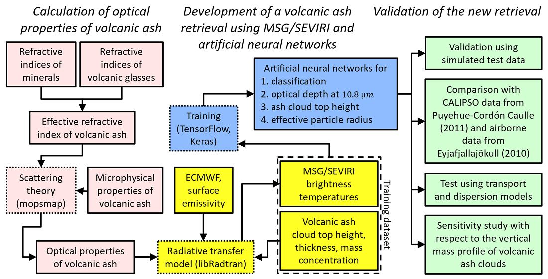
The New Volcanic Ash Satellite Retrieval VACOS Using MSG/SEVIRI and Artificial Neural Networks: 1. Development

 ,
,
Abstract
: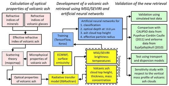
1. Introduction
2. MSG/SEVIRI
3. VADUGS
4. Training Dataset
4.1. Input Data
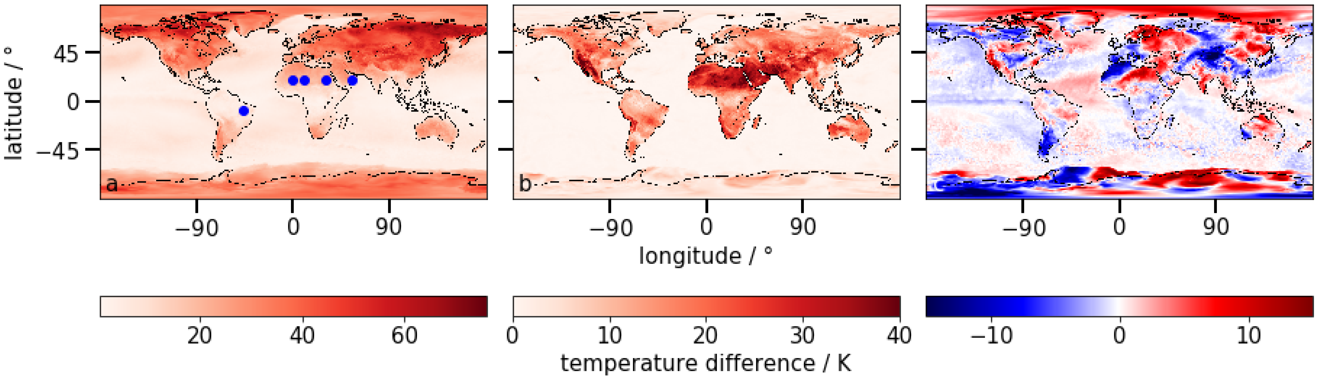
4.1.1. Surface Emissivity
4.1.2. Atmospheric Data
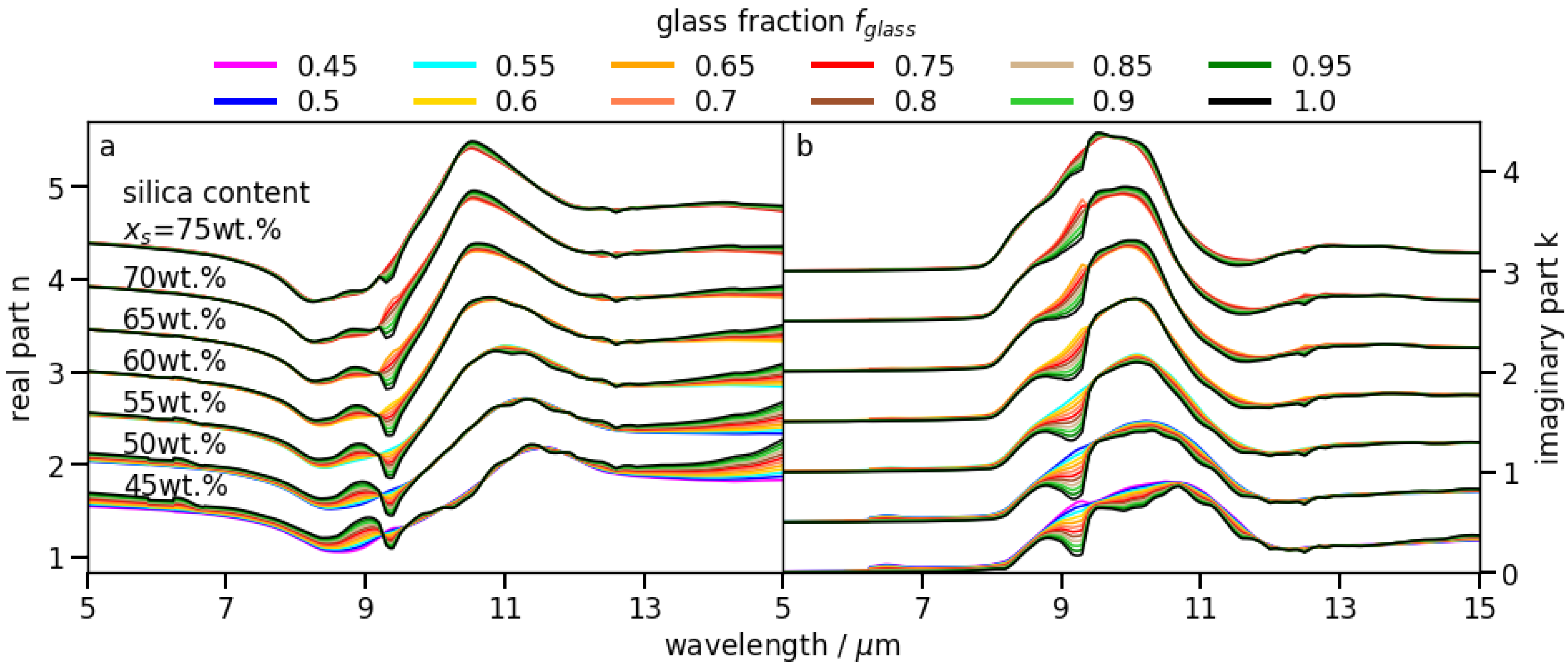
4.1.3. Volcanic Ash Clouds
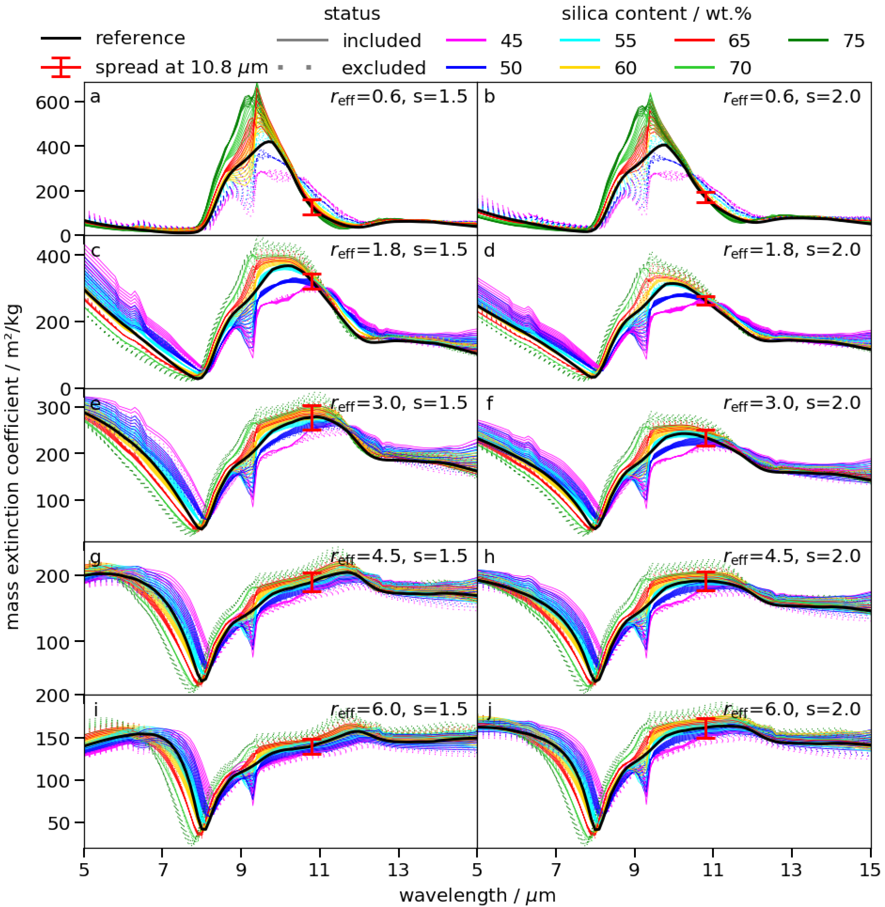
4.2. Radiative Transfer Calculations
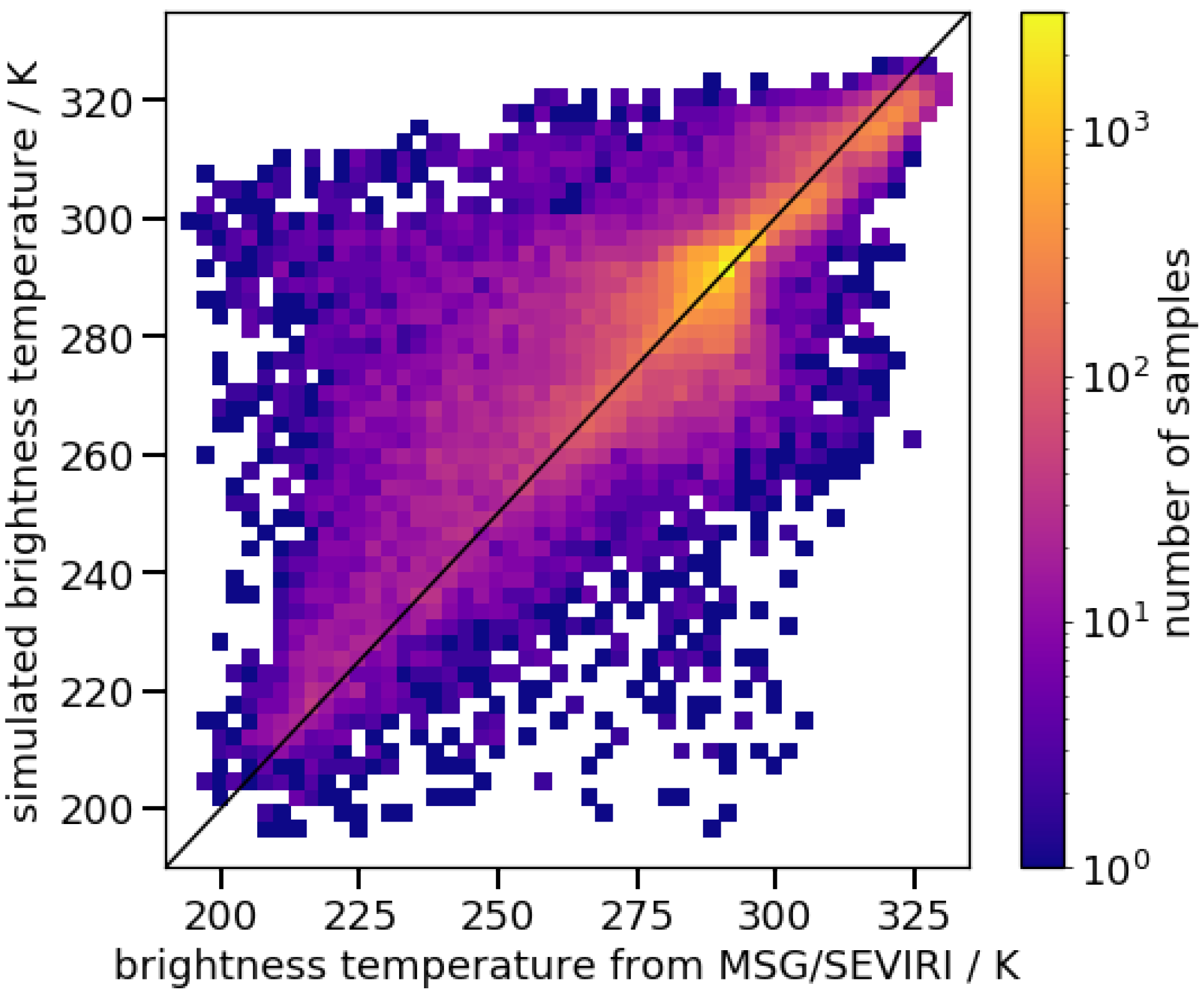
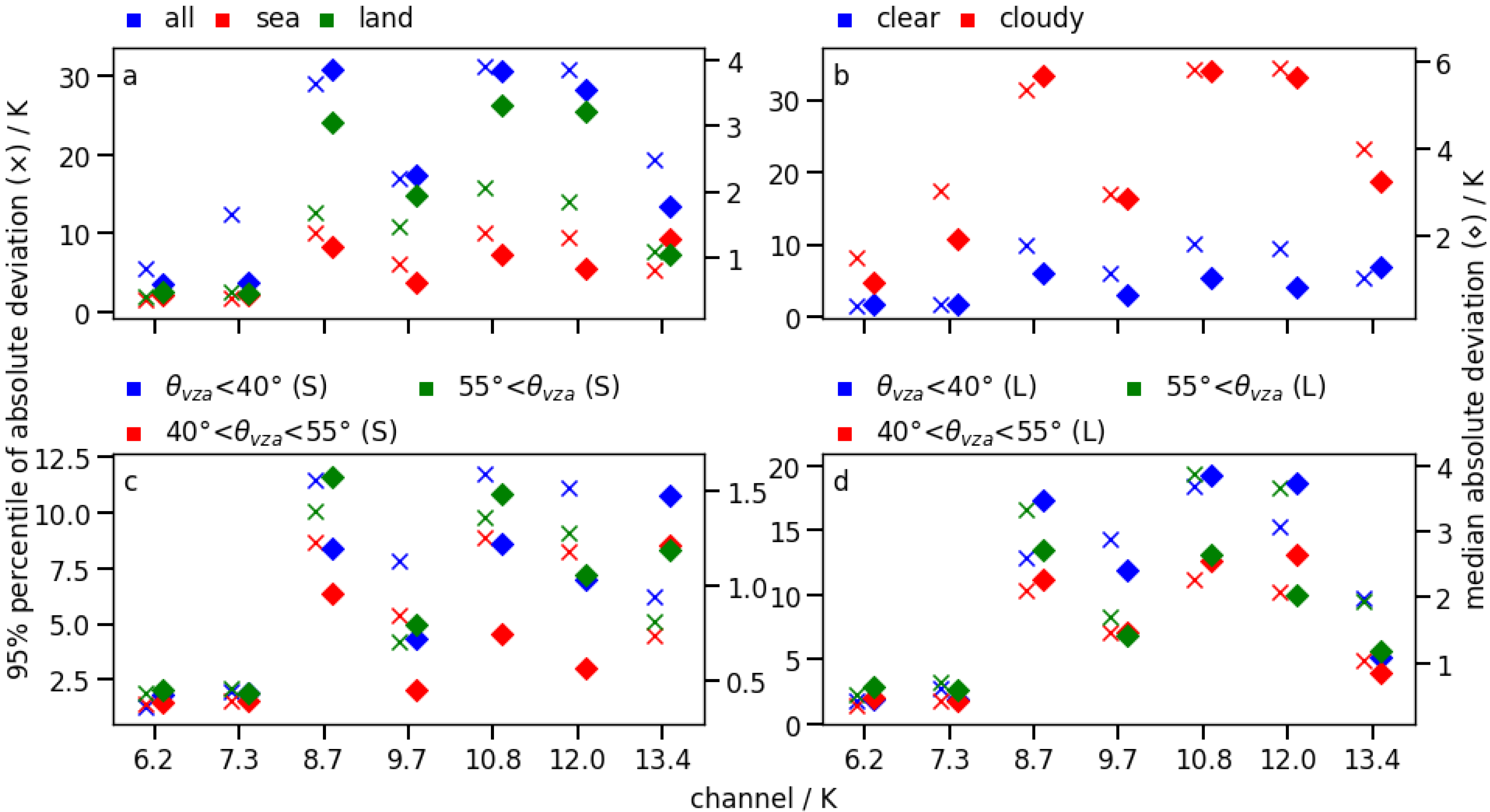
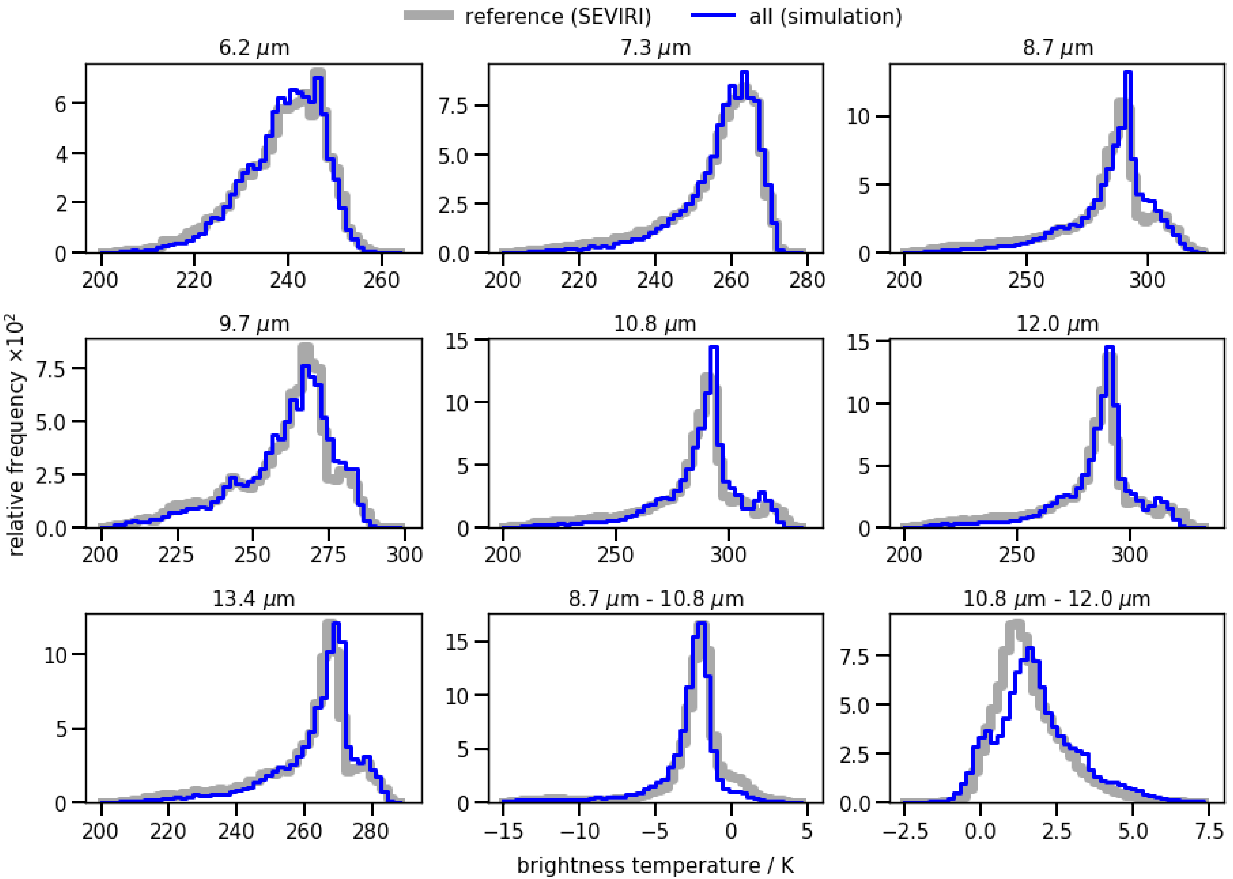
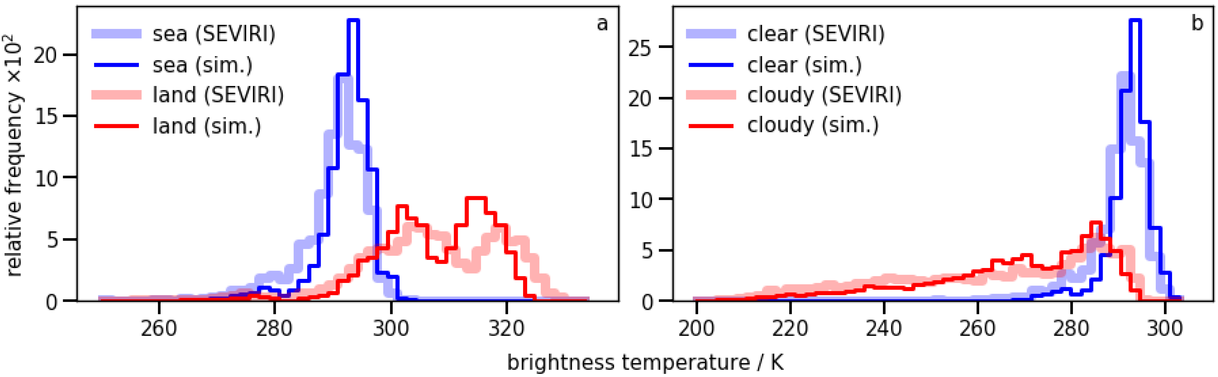
4.3. Test of the Ash-Free Training Data
4.4. Training, Validation and Test Data
5. Training of the ANNs
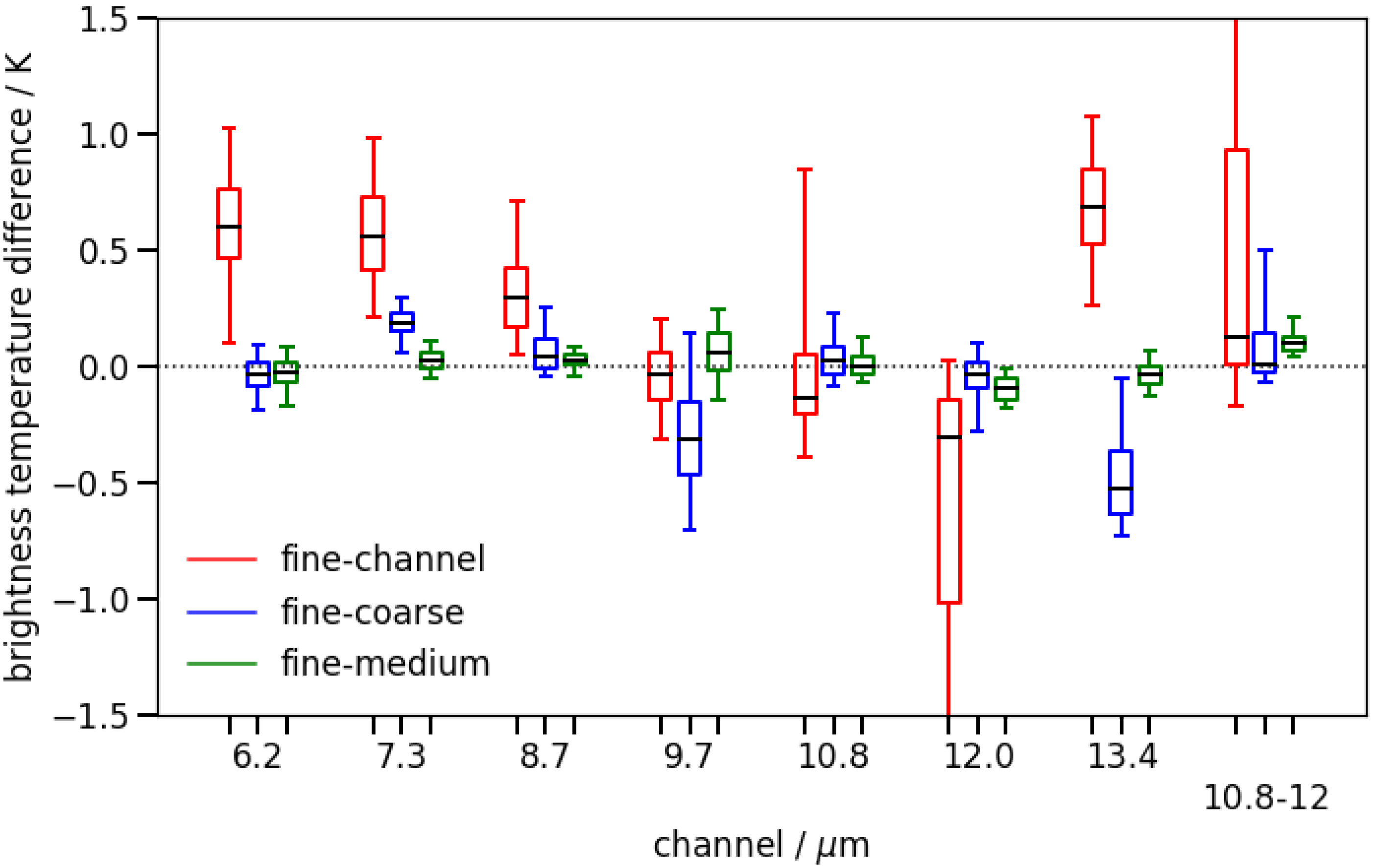
6. Notes on the Application
7. Conclusions
Author Contributions
Funding
Institutional Review Board Statement
Informed Consent Statement
Data Availability Statement
Acknowledgments
Conflicts of Interest
References
- Siebert, L.; Simkin, T.; Kimberly, P. Volcanoes of the World, 3rd ed.; University of California Press: Berkeley, CA, USA; Los Angeles, CA, USA; London, UK, 2011. [Google Scholar]
- Wilson, T.M.; Stewart, C.; Sword-Daniels, V.; Leonard, G.S.; Johnston, D.M.; Cole, J.W.; Wardman, J.; Wilson, G.; Barnard, S.T. Volcanic ash impacts on critical infrastructure. Phys. Chem. Earth 2012, 45–46, 5–23. [Google Scholar] [CrossRef]
- Casadevall, T.J. The 1989–1990 eruption of Redoubt Volcano, Alaska: Impacts on aircraft operations. J. Volcanol. Geotherm. Res. 1994, 62, 301–316. [Google Scholar] [CrossRef]
- Guffanti, M.; Casadevall, T.J.; Budding, K. Encounters of aircraft with volcanic ash clouds; A compilation of known incidents, 1953–2009. U.S. Geological Survey Data Series 545, Ver. 1.0, 12 p., Plus 4 Appendixes Including the Compilation Database. 2010. Available online: https://pubs.usgs.gov/ds/545/DS545.pdf (accessed on 5 August 2021).
- Weinzierl, B.; Sauer, D.; Minikin, A.; Reitebuch, O.; Dahlkötter, F.; Mayer, B.; Emde, C.; Tegen, I.; Gasteiger, J.; Petzold, A.; et al. On the visibility of airborne volcanic ash and mineral dust from the pilot’s perspective in flight. Phys. Chem. Earth Parts A B C 2012, 45–46, 87–102. [Google Scholar] [CrossRef] [Green Version]
- Schumann, U.; Weinzierl, B.; Reitebuch, O.; Schlager, H.; Minikin, A.; Forster, C.; Baumann, R.; Sailer, T.; Graf, K.; Mannstein, H.; et al. Airborne observations of the Eyjafjalla volcano ash cloud over Europe during air space closure in April and May 2010. Atmos. Chem. Phys 2011, 11, 2245–2279. [Google Scholar] [CrossRef] [Green Version]
- Budd, L.; Griggs, S.; Howarth, D.; Ison, S. A Fiasco of Volcanic Proportions? Eyjafjallajökull and the Closure of European Airspace. Mobilities 2011, 6, 31–40. [Google Scholar] [CrossRef]
- Pavolonis, M.J.; Sieglaff, J.; Cintineo, J. Spectrally Enhanced Cloud Objects—A generalized framework for automated detection of volcanic ash and dust clouds using passive satellite measurements: 1. Multispectral analysis. J. Geophys. Res. Atmos. 2015, 120, 7813–7841. [Google Scholar] [CrossRef]
- Volcanic Ash Contingency Plan: European and North Atlantic Regions, Edition 2.0.0. International Civil Aviation Organization, European and North Atlantic Office. 2016. Available online: https://www.skybrary.aero/bookshelf/books/357.pdf (accessed on 5 August 2021).
- Langmann, B. Volcanic Ash versus Mineral Dust: Atmospheric Processing and Environmental and Climate Impacts. ISRN Atmos. Sci. 2013, 2013, 245076. [Google Scholar] [CrossRef] [Green Version]
- Watkin, S.C. The application of AVHRR data for the detection of volcanic ash in a Volcanic Ash Advisory Centre. Meteorol. Appl. 2003, 10, 301–311. [Google Scholar] [CrossRef]
- Stohl, A.; Prata, A.J.; Eckhardt, S.; Clarisse, L.; Durant, A.; Henne, S.; Kristiansen, N.I.; Minikin, A.; Schumann, U.; Seibert, P.; et al. Determination of time- and height-resolved volcanic ash emissions and their use for quantitative ash dispersion modeling: The 2010 Eyjafjallajökull eruption. Atmos. Chem. Phys. 2011, 11, 4333–4351. [Google Scholar] [CrossRef] [Green Version]
- Dacre, H.F.; Harvey, N.J.; Webley, P.W.; Morton, D. How accurate are volcanic ash simulations of the 2010 Eyjafjallajökull eruption? J. Geophys. Res. Atmos. 2016, 121, 3534–3547. [Google Scholar] [CrossRef] [Green Version]
- Winker, D.M.; Liu, Z.; Omar, A.; Tackett, J.; Fairlie, D. CALIOP observations of the transport of ash from the Eyjafjallajökull volcano in April 2010. J. Geophys. Res. Atmos. 2012, 117. [Google Scholar] [CrossRef]
- Winker, D.M.; Vaughan, M.A.; Omar, A.; Hu, Y.; Powell, K.A.; Liu, Z.; Hunt, W.H.; Young, S.A. Overview of the CALIPSO Mission and CALIOP Data Processing Algorithms. J. Atmos. Ocean. Technol. 2009, 26, 2310–2323. [Google Scholar] [CrossRef]
- Jurkat, T.; Voigt, C.; Arnold, F.; Schlager, H.; Aufmhoff, H.; Schmale, J.; Schneider, J.; Lichtenstern, M.; Dörnbrack, A. Airborne stratospheric ITCIMS measurements of SO2, HCl, and HNO3 in the aged plume of volcano Kasatochi. J. Geophys. Res. Atmos. 2010, 115. [Google Scholar] [CrossRef] [Green Version]
- Schmale, J.; Schneider, J.; Jurkat, T.; Voigt, C.; Kalesse, H.; Rautenhaus, M.; Lichtenstern, M.; Schlager, H.; Ancellet, G.; Arnold, F.; et al. Aerosol layers from the 2008 eruptions of Mount Okmok and Mount Kasatochi: In situ upper troposphere and lower stratosphere measurements of sulfate and organics over Europe. J. Geophys. Res. Atmos. 2010, 115. [Google Scholar] [CrossRef] [Green Version]
- Marenco, F.; Johnson, B.; Turnbull, K.; Newman, S.; Haywood, J.; Webster, H.; Ricketts, H. Airborne lidar observations of the 2010 Eyjafjallajökull volcanic ash plume. J. Geophys. Res. Atmos. 2011, 116. [Google Scholar] [CrossRef]
- Weber, K.; Eliasson, J.; Vogel, A.; Fischer, C.; Pohl, T.; van Haren, G.; Meier, M.; Grobéty, B.; Dahmann, D. Airborne in-situ investigations of the Eyjafjallajökull volcanic ash plume on Iceland and over north-western Germany with light aircrafts and optical particle counters. Atmos. Environ. 2012, 48, 9–21. [Google Scholar] [CrossRef]
- Voigt, C.; Jessberger, P.; Jurkat, T.; Kaufmann, S.; Baumann, R.; Schlager, H.; Bobrowski, N.; Giuffrida, G.; Salerno, G. Evolution of CO2, SO2, HCl, and HNO3 in the volcanic plumes from Etna. Geophys. Res. Lett. 2014, 41, 2196–2203. [Google Scholar] [CrossRef] [Green Version]
- Shcherbakov, V.; Jourdan, O.; Voigt, C.; Gayet, J.F.; Chauvigne, A.; Schwarzenboeck, A.; Minikin, A.; Klingebiel, M.; Weigel, R.; Borrmann, S.; et al. Etna and Mt. Stromboli. Atmos. Chem. Phys. 2016, 16, 11883–11897. [Google Scholar] [CrossRef] [Green Version]
- Wen, S.; Rose, W.I. Retrieval of sizes and total masses of particles in volcanic clouds using AVHRR bands 4 and 5. J. Geophys. Res. Atmos. 1994, 99, 5421–5431. [Google Scholar] [CrossRef]
- Piontek, D.; Hornby, A.; Voigt, C.; Bugliaro, L.; Gasteiger, J. Determination of complex refractive indices and optical properties of volcanic ashes in the thermal infrared based on generic petrological compositions. J. Volcanol. Geotherm. Res. 2021, 411, 107174. [Google Scholar] [CrossRef]
- Prata, A.J. Infrared radiative transfer calculations for volcanic ash clouds. Geophys. Res. Lett. 1989, 16, 1293–1296. [Google Scholar] [CrossRef]
- Prata, A.J. Observations of volcanic ash clouds in the 10–12 μm window using AVHRR/2 data. Int. J. Remote Sens. 1989, 10, 751–761. [Google Scholar] [CrossRef]
- Inoue, T. On the Temperature and Effective Emissivity Determination of Semi-Transparent Cirrus Clouds by Bi-Spectral Measurements in the 10 μm Window Region. J. Meteorol. Soc. Jpn. 1985, 63, 88–99. [Google Scholar] [CrossRef] [Green Version]
- Yu, T.; Rose, W.I.; Prata, A.J. Atmospheric correction for satellite-based volcanic ash mapping and retrievals using “split window” IR data from GOES and AVHRR. J. Geophys. Res. Atmos. 2002, 107, AAC 10-1–AAC 10-19. [Google Scholar] [CrossRef]
- Ackerman, S.A. Remote sensing aerosols using satellite infrared observations. J. Geophys. Res. Atmos. 1997, 102, 17069–17079. [Google Scholar] [CrossRef]
- Clarisse, L.; Prata, F.; Lacour, J.L.; Hurtmans, D.; Clerbaux, C.; Coheur, P.F. A correlation method for volcanic ash detection using hyperspectral infrared measurements. Geophys. Res. Lett. 2010, 37. [Google Scholar] [CrossRef] [Green Version]
- Gangale, G.; Prata, A.; Clarisse, L. The infrared spectral signature of volcanic ash determined from high-spectral resolution satellite measurements. Remote Sens. Environ. 2010, 114, 414–425. [Google Scholar] [CrossRef]
- Francis, P.N.; Cooke, M.C.; Saunders, R.W. Retrieval of physical properties of volcanic ash using Meteosat: A case study from the 2010 Eyjafjallajökull eruption. J. Geophys. Res. Atmos. 2012, 117. [Google Scholar] [CrossRef]
- Guéhenneux, Y.; Gouhier, M.; Labazuy, P. Improved space borne detection of volcanic ash for real-time monitoring using 3-Band method. J. Volcanol. Geotherm. Res. 2015, 293, 25–45. [Google Scholar] [CrossRef]
- Prata, A.J.; Grant, I.F. Retrieval of microphysical and morphological properties of volcanic ash plumes from satellite data: Application to Mt Ruapehu, New Zealand. Q. J. R. Meteorol. Soc. 2001, 127, 2153–2179. [Google Scholar] [CrossRef]
- Pavolonis, M.J.; Feltz, W.F.; Heidinger, A.K.; Gallina, G.M. A Daytime Complement to the Reverse Absorption Technique for Improved Automated Detection of Volcanic Ash. J. Atmos. Ocean. Technol. 2006, 23, 1422–1444. [Google Scholar] [CrossRef]
- Zhu, L.; Liu, J.; Liu, C.; Wang, M. Satellite remote sensing of volcanic ash cloud in complicated meteorological conditions. Sci. China Earth Sci. 2011, 54, 1789–1795. [Google Scholar] [CrossRef]
- Pavolonis, M.J. Advances in Extracting Cloud Composition Information from Spaceborne Infrared Radiances—A Robust Alternative to Brightness Temperatures. Part I: Theory. J. Appl. Meteorol. Climatol. 2010, 49, 1992–2012. [Google Scholar] [CrossRef]
- Pavolonis, M.J.; Heidinger, A.K.; Sieglaff, J. Automated retrievals of volcanic ash and dust cloud properties from upwelling infrared measurements. J. Geophys. Res. Atmos. 2013, 118, 1436–1458. [Google Scholar] [CrossRef]
- Grainger, R.G.; Peters, D.M.; Thomas, G.E.; Smith, A.J.A.; Siddans, R.; Carboni, E.; Dudhia, A. Measuring volcanic plume and ash properties from space. Geol. Soc. Lond. Spec. Publ. 2013, 380, 293–320. [Google Scholar] [CrossRef] [Green Version]
- Carn, S.A.; Krueger, A.J.; Krotkov, N.A.; Yang, K.; Evans, K. Tracking volcanic sulfur dioxide clouds for aviation hazard mitigation. Nat. Hazards 2009, 51, 325–343. [Google Scholar] [CrossRef]
- Thomas, H.E.; Prata, A.J. Sulphur dioxide as a volcanic ash proxy during the April-May 2010 eruption of Eyjafjallajökull Volcano, Iceland. Atmos. Chem. Phys. 2011, 11, 6871–6880. [Google Scholar] [CrossRef] [Green Version]
- Sears, T.M.; Thomas, G.E.; Carboni, E.A.; Smith, A.J.; Grainger, R.G. SO2 as a possible proxy for volcanic ash in aviation hazard avoidance. J. Geophys. Res. Atmos. 2013, 118, 5698–5709. [Google Scholar] [CrossRef]
- Prata, A.J.; Kerkmann, J. Simultaneous retrieval of volcanic ash and SO2 using MSG-SEVIRI measurements. Geophys. Res. Lett. 2007, 34. [Google Scholar] [CrossRef] [Green Version]
- Prata, A.J.; Grant, I.F. Determination of mass loadings and plume heights of volcanic ash clouds from satellite data. CSIRO Atmos. Res. Tech. Pap. 2001, 48, 1–41. [Google Scholar]
- Rodgers, C.D. Inverse Methods for Atmospheric Sounding; World Scientific: Singapore; River Edge, NJ, USA; London, UK, 2000. [Google Scholar] [CrossRef]
- Pugnaghi, S.; Guerrieri, L.; Corradini, S.; Merucci, L.; Arvani, B. A new simplified approach for simultaneous retrieval of SO2 and ash content of tropospheric volcanic clouds: An application to the Mt Etna volcano. Atmos. Meas. Tech. 2013, 6, 1315–1327. [Google Scholar] [CrossRef] [Green Version]
- Schneider, D.J.; Van Eaton, A.R.; Wallace, K.L. Satellite observations of the 2016–2017 eruption of Bogoslof volcano: Aviation and ash fallout hazard implications from a water-rich eruption. Bull. Volcanol. 2020, 82, 29. [Google Scholar] [CrossRef]
- Prata, A.; Turner, P. Cloud-top height determination using ATSR data. Remote Sens. Environ. 1997, 59, 1–13. [Google Scholar] [CrossRef]
- Menzel, W.P.; Smith, W.L.; Stewart, T.R. Improved Cloud Motion Wind Vector and Altitude Assignment Using VAS. J. Clim. Appl. Meteorol. 1983, 22, 377–384. [Google Scholar] [CrossRef]
- Taylor, I.A.; Carboni, E.; Ventress, L.J.; Mather, T.A.; Grainger, R.G. An adaptation of the CO2 slicing technique for the Infrared Atmospheric Sounding Interferometer to obtain the height of tropospheric volcanic ash clouds. Atmos. Meas. Tech. 2019, 12, 3853–3883. [Google Scholar] [CrossRef] [Green Version]
- Hornik, K.; Stinchcombe, M.; White, H. Multilayer feedforward networks are universal approximators. Neural Netw. 1989, 2, 359–366. [Google Scholar] [CrossRef]
- Hsieh, W.W.; Tang, B. Applying Neural Network Models to Prediction and Data Analysis in Meteorology and Oceanography. Bull. Am. Meteorol. Soc. 1998, 79, 1855–1870. [Google Scholar] [CrossRef]
- Gardner, M.; Dorling, S. Artificial neural networks (the multilayer perceptron)—A review of applications in the atmospheric sciences. Atmos. Environ. 1998, 32, 2627–2636. [Google Scholar] [CrossRef]
- Cerdeña, A.; González, A.; Pérez, J.C. Remote Sensing of Water Cloud Parameters Using Neural Networks. J. Atmos. Ocean. Technol. 2007, 24, 52–63. [Google Scholar] [CrossRef]
- Minnis, P.; Hong, G.; Sun-Mack, S.; Smith, W.L., Jr.; Chen, Y.; Miller, S.D. Estimating nocturnal opaque ice cloud optical depth from MODIS multispectral infrared radiances using a neural network method. J. Geophys. Res. Atmos. 2016, 121, 4907–4932. [Google Scholar] [CrossRef] [Green Version]
- Kox, S.; Bugliaro, L.; Ostler, A. Retrieval of cirrus cloud optical thickness and top altitude from geostationary remote sensing. Atmos. Meas. Tech. 2014, 7, 3233–3246. [Google Scholar] [CrossRef] [Green Version]
- Holl, G.; Eliasson, S.; Mendrok, J.; Buehler, S.A. SPARE-ICE: Synergistic ice water path from passive operational sensors. J. Geophys. Res. Atmos. 2014, 119, 1504–1523. [Google Scholar] [CrossRef]
- Xu, J.; Schüssler, O.; Rodriguez, D.G.L.; Romahn, F.; Doicu, A. A Novel Ozone Profile Shape Retrieval Using Full-Physics Inverse Learning Machine (FP-ILM). IEEE J. Sel. Top. Appl. Earth Obs. Remote Sens. 2017, 10, 5442–5457. [Google Scholar] [CrossRef] [Green Version]
- Piscini, A.; Carboni, E.; Del Frate, F.; Grainger, R.G. Simultaneous retrieval of volcanic sulphur dioxide and plume height from hyperspectral data using artificial neural networks. Geophys. J. Int. 2014, 198, 697–709. [Google Scholar] [CrossRef] [Green Version]
- Efremenko, D.S.; Loyola, R.D.G.; Hedelt, P.; Spurr, R.J.D. Volcanic SO2 plume height retrieval from UV sensors using a full-physics inverse learning machine algorithm. Int. J. Remote Sens. 2017, 38, 1–27. [Google Scholar] [CrossRef] [Green Version]
- Hedelt, P.; Efremenko, D.S.; Loyola, D.G.; Spurr, R.; Clarisse, L. Sulfur dioxide layer height retrieval from Sentinel-5 Precursor/TROPOMI using FP_ILM. Atmos. Meas. Tech. 2019, 12, 5503–5517. [Google Scholar] [CrossRef] [Green Version]
- Loyola, D.G.; Xu, J.; Heue, K.P.; Zimmer, W. Applying FP_ILM to the retrieval of geometry-dependent effective Lambertian equivalent reflectivity (GE_LER) daily maps from UVN satellite measurements. Atmos. Meas. Tech. 2020, 13, 985–999. [Google Scholar] [CrossRef] [Green Version]
- Gray, T.M.; Bennartz, R. Automatic volcanic ash detection from MODIS observations using a back-propagation neural network. Atmos. Meas. Tech. 2015, 8, 5089–5097. [Google Scholar] [CrossRef] [Green Version]
- Watson, I.; Realmuto, V.; Rose, W.; Prata, A.; Bluth, G.; Gu, Y.; Bader, C.; Yu, T. Thermal infrared remote sensing of volcanic emissions using the moderate resolution imaging spectroradiometer. J. Volcanol. Geotherm. Res. 2004, 135, 75–89. [Google Scholar] [CrossRef]
- Picchiani, M.; Chini, M.; Corradini, S.; Merucci, L.; Sellitto, P.; Del Frate, F.; Stramondo, S. Volcanic ash detection and retrievals using MODIS data by means of neural networks. Atmos. Meas. Tech. 2011, 4, 2619–2631. [Google Scholar] [CrossRef] [Green Version]
- Picchiani, M.; Chini, M.; Corradini, S.; Merucci, L.; Piscini, A.; Frate, F.D. Neural network multispectral satellite images classification of volcanic ash plumes in a cloudy scenario. Ann. Geophys. 2014, 57. [Google Scholar] [CrossRef]
- Piscini, A.; Picchiani, M.; Chini, M.; Corradini, S.; Merucci, L.; Del Frate, F.; Stramondo, S. A neural network approach for the simultaneous retrieval of volcanic ash parameters and SO2 using MODIS data. Atmos. Meas. Tech. 2014, 7, 4023–4047. [Google Scholar] [CrossRef] [Green Version]
- Corradini, S.; Pugnaghi, S.; Piscini, A.; Guerrieri, L.; Merucci, L.; Picchiani, M.; Chini, M. Volcanic Ash and SO2 retrievals using synthetic MODIS TIR data: Comparison between inversion procedures and sensitivity analysis. Ann. Geophys. 2014, 57. [Google Scholar] [CrossRef] [Green Version]
- Zhu, W.; Zhu, L.; Li, J.; Sun, H. Retrieving volcanic ash top height through combined polar orbit active and geostationary passive remote sensing data. Remote Sens. 2020, 12, 953. [Google Scholar] [CrossRef] [Green Version]
- Schmetz, J.; Pili, P.; Tjemkes, S.; Just, D.; Kerkmann, J.; Rota, S.; Ratier, A. An Introduction to Meteosat Second Generation (MSG). Bull. Am. Meteorol. Soc. 2002, 83, 977–992. [Google Scholar] [CrossRef]
- Kox, S.; Schmidl, M.; Graf, K.; Mannstein, H.; Buras, R.; Gasteiger, J. A new approach on the detection of volcanic ash clouds. In Proceedings of the 2013 EUMETSAT Meteorological Satellite Conference, Vienna, Austria, 16–20 September 2013. [Google Scholar]
- Bugliaro, L.; Piontek, D.; Kox, S.; Schmidl, M.; Mayer, B.; Müller, R.; Vázquez-Navarro, M.; Gasteiger, J.; Kar, J. Combining radiative transfer calculations and a neural network for the remote sensing of volcanic ash using MSG/SEVIRI. 2021. in preparation. [Google Scholar]
- Jahresbericht 2015: Flugwetterdienst Deutscher Wetterdienst. 2015. Available online: https://www.dwd.de/DE/fachnutzer/luftfahrt/download/jahresberichte_flugwetterdienst/2015.pdf?__blob=publicationFile&v=3 (accessed on 5 August 2021).
- Meeting on the Intercomparison of Satellite-based Volcanic Ash Retrieval Algorithms, Madison WI, USA, 29 June—2 July 2015, Final Report. World Meteorological Organization. 2015. Available online: https://web.archive.org/web/20171113102551/http://www.wmo.int/pages/prog/sat/documents/SCOPE-NWC-PP2_VAIntercompWSReport2015.pdf (accessed on 5 August 2021).
- Reed, B.E.; Peters, D.M.; McPheat, R.; Grainger, R.G. The Complex Refractive Index of Volcanic Ash Aerosol Retrieved From Spectral Mass Extinction. J. Geophys. Res. Atmos. 2018, 123, 1339–1350. [Google Scholar] [CrossRef] [Green Version]
- Deguine, A.; Petitprez, D.; Clarisse, L.; Guđmundsson, S.; Outes, V.; Villarosa, G.; Herbin, H. Complex refractive index of volcanic ash aerosol in the infrared, visible, and ultraviolet. Appl. Opt. 2020, 59, 884–895. [Google Scholar] [CrossRef] [PubMed]
- Western, L.M.; Watson, M.I.; Francis, P.N. Uncertainty in two-channel infrared remote sensing retrievals of a well-characterised volcanic ash cloud. Bull. Volcanol. 2015, 77, 67. [Google Scholar] [CrossRef] [Green Version]
- Prata, G.S.; Ventress, L.J.; Carboni, E.; Mather, T.A.; Grainger, R.G.; Pyle, D.M. A New Parameterization of Volcanic Ash Complex Refractive Index Based on NBO/T and SiO2 Content. J. Geophys. Res. Atmos. 2019, 124, 1779–1797. [Google Scholar] [CrossRef] [Green Version]
- Strandgren, J.; Bugliaro, L.; Sehnke, F.; Schröder, L. Cirrus cloud retrieval with MSG/SEVIRI using artificial neural networks. Atmos. Meas. Tech. 2017, 10, 3547–3573. [Google Scholar] [CrossRef] [Green Version]
- Strandgren, J.; Fricker, J.; Bugliaro, L. Characterisation of the artificial neural network CiPS for cirrus cloud remote sensing with MSG/SEVIRI. Atmos. Meas. Tech. 2017, 10, 4317–4339. [Google Scholar] [CrossRef] [Green Version]
- Piontek, D.; Bugliaro, L.; Jayanta, K.; Schumann, U.; Marenco, F.; Plu, M.; Voigt, C. The New Volcanic Ash Retrieval VACOS Using MSG/SEVIRI and Artificial Neural Networks: 2. Validation. Remote Sens. 2021. submitted. [Google Scholar]
- ESA. Available online: https://directory.eoportal.org/web/eoportal/satellite-missions/m/meteosat-second-generation (accessed on 29 June 2020).
- WMO. Available online: https://www.wmo-sat.info/oscar/satellites/view/303 (accessed on 29 June 2020).
- Schmit, T.J.; Gunshor, M.M.; Menzel, W.P.; Gurka, J.J.; Li, J.; Bachmeier, A.S. Introducing the Next-Generation Advanced Baseline Imager on GOES-R. Bull. Am. Meteorol. Soc. 2005, 86, 1079–1096. [Google Scholar] [CrossRef]
- Durand, Y.; Hallibert, P.; Wilson, M.; Lekouara, M.; Grabarnik, S.; Aminou, D.; Blythe, P.; Napierala, B.; Canaud, J.L.; Pigouche, O.; et al. The flexible combined imager onboard MTG: From design to calibration. In Sensors, Systems, and Next-Generation Satellites XIX; Meynart, R., Neeck, S.P., Shimoda, H., Eds.; International Society for Optics and Photonics, SPIE: Bellingham, WA, USA, 2015; Volume 9639, pp. 1–14. [Google Scholar] [CrossRef]
- Bessho, K.; Date, K.; Hayashi, M.; Ikeda, A.; Imai, T.; Inoue, H.; Kumagai, Y.; Miyakawa, T.; Murata, H.; Ohno, T.; et al. An Introduction to Himawari-8/9-Japan’s New-Generation Geostationary Meteorological Satellites. J. Meteorol. Soc. Jpn. Ser. II 2016, 94, 151–183. [Google Scholar] [CrossRef] [Green Version]
- Yang, J.; Zhang, Z.; Wei, C.; Lu, F.; Guo, Q. Introducing the New Generation of Chinese Geostationary Weather Satellites, Fengyun-4. Bull. Am. Meteorol. Soc. 2017, 98, 1637–1658. [Google Scholar] [CrossRef]
- Montavon, G.; Orr, G.B.; Müller, K.R. (Eds.) Neural Networks: Tricks of the Trade, 2nd ed.; Springer: Berlin/Heidelberg, Germany, 2012. [Google Scholar] [CrossRef]
- Zhou, D.K.; Larar, A.M.; Liu, X.; Smith, W.L.; Strow, L.L.; Yang, P.; Schlüssel, P.; Calbet, X. Global Land Surface Emissivity Retrieved From Satellite Ultraspectral IR Measurements. IEEE Trans. Geosci. Remote Sens. 2011, 49, 1277–1290. [Google Scholar] [CrossRef]
- Zhou, D.K.; Larar, A.M.; Liu, X. MetOp-A/IASI Observed Continental Thermal IR Emissivity Variations. IEEE J. Sel. Top. Appl. Earth Obs. Remote Sens. 2013, 6, 1156–1162. [Google Scholar] [CrossRef]
- Zhou, D.K.; Larar, A.M.; Liu, X. On the relationship between land surface infrared emissivity and soil moisture. J. Appl. Remote Sens. 2018, 12, 1–14. [Google Scholar] [CrossRef] [Green Version]
- Masuda, K.; Takashima, T.; Takayama, Y. Emissivity of pure and sea waters for the model sea surface in the infrared window regions. Remote Sens. Environ. 1988, 24, 313–329. [Google Scholar] [CrossRef]
- Wu, X.; Smith, W.L. Emissivity of rough sea surface for 8–13 μm: Modeling and verification. Appl. Opt. 1997, 36, 2609–2619. [Google Scholar] [CrossRef]
- Niclòs, R.; Valor, E.; Caselles, V.; Coll, C.; Sánchez, J.M. In situ angular measurements of thermal infrared sea surface emissivity—Validation of models. Remote Sens. Environ. 2005, 94, 83–93. [Google Scholar] [CrossRef]
- Masuda, K. Infrared sea surface emissivity including multiple reflection effect for isotropic Gaussian slope distribution model. Remote Sens. Environ. 2006, 103, 488–496. [Google Scholar] [CrossRef]
- Labed, J.; Stoll, M.P. Angular variation of land surface spectral emissivity in the thermal infrared: Laboratory investigations on bare soils. Int. J. Remote Sens. 1991, 12, 2299–2310. [Google Scholar] [CrossRef]
- Snyder, W.C.; Wan, Z.; Zhang, Y.; Feng, Y.Z. Thermal Infrared (3–14 μm) bidirectional reflectance measurements of sands and soils. Remote Sens. Environ. 1997, 60, 101–109. [Google Scholar] [CrossRef]
- Sobrino, J.A.; Cuenca, J. Angular variation of thermal infrared emissivity for some natural surfaces from experimental measurements. Appl. Opt. 1999, 38, 3931–3936. [Google Scholar] [CrossRef] [PubMed]
- Cuenca, J.; Sobrino, J.A. Experimental measurements for studying angular and spectral variation of thermal infrared emissivity. Appl. Opt. 2004, 43, 4598–4602. [Google Scholar] [CrossRef]
- McAtee, B.K.; Prata, A.J.; Lynch, M.J. The Angular Behavior of Emitted Thermal Infrared Radiation (8–12 μm) at a Semiarid Site. J. Appl. Meteorol. 2003, 42, 1060–1071. [Google Scholar] [CrossRef]
- García-Santos, V.; Valor, E.; Caselles, V.; Ángeles Burgos, M.; Coll, C. On the angular variation of thermal infrared emissivity of inorganic soils. J. Geophys. Res. Atmos. 2012, 117. [Google Scholar] [CrossRef] [Green Version]
- Hersbach, H.; Bell, B.; Berrisford, P.; Hirahara, S.; Horányi, A.; Muñoz-Sabater, J.; Nicolas, J.; Peubey, C.; Radu, R.; Schepers, D.; et al. The ERA5 global reanalysis. Q. J. R. Meteorol. Soc. 2020, 146, 1999–2049. [Google Scholar] [CrossRef]
- ECMWF. Available online: https://confluence.ecmwf.int/display/CKB/ERA5%3A+data+documentation (accessed on 30 June 2020).
- Reineke, W.; Schlömann, M. Globale Umwelt. Klima und Mikroorganismen. In Umweltmikrobiologie; Springer: Berlin/Heidelberg, Germany, 2020; pp. 1–34. [Google Scholar] [CrossRef]
- Friedlingstein, P.; O’Sullivan, M.; Jones, M.W.; Andrew, R.M.; Hauck, J.; Olsen, A.; Peters, G.P.; Peters, W.; Pongratz, J.; Sitch, S.; et al. Global Carbon Budget 2020. Earth Syst. Sci. Data 2020, 12, 3269–3340. [Google Scholar] [CrossRef]
- Chan, K.; Chan, K. Aerosol optical depths and their contributing sources in Taiwan. Atmos. Environ. 2017, 148, 364–375. [Google Scholar] [CrossRef]
- Chan, K. Biomass burning sources and their contributions to the local air quality in Hong Kong. Sci. Total Environ. 2017, 596–597, 212–221. [Google Scholar] [CrossRef]
- Mayer, B.; Kylling, A.; Emde, C.; Buras, R.; Hamann, U.; Gasteiger, J.; Richter, B. libRadtrans Users’s Guide. 2019. Available online: https://web.archive.org/web/20200822040829/http://www.libradtran.org/doc/libRadtran.pdf (accessed on 5 August 2021).
- Wallace, J.; Hobbs, P. Atmospheric Science: An Introductory Survey, 2nd ed.; Academic Press: Burlington, MA, USA, 2006. [Google Scholar]
- Bugliaro, L.; Zinner, T.; Keil, C.; Mayer, B.; Hollmann, R.; Reuter, M.; Thomas, W. Validation of cloud property retrievals with simulated satellite radiances: A case study for SEVIRI. Atmos. Chem. Phys. 2011, 11, 5603–5624. [Google Scholar] [CrossRef] [Green Version]
- Hu, Y.X.; Stamnes, K. An Accurate Parameterization of the Radiative Properties of Water Clouds Suitable for Use in Climate Models. J. Clim. 1993, 6, 728–742. [Google Scholar] [CrossRef] [Green Version]
- Wyser, K. The Effective Radius in Ice Clouds. J. Clim. 1998, 11, 1793–1802. [Google Scholar] [CrossRef]
- Heymsfield, A.J.; Schmitt, C.; Bansemer, A. Ice Cloud Particle Size Distributions and Pressure-Dependent Terminal Velocities from In Situ Observations at Temperatures from 0 °C to −86 °C. J. Atmos. Sci. 2013, 70, 4123–4154. [Google Scholar] [CrossRef]
- Yang, P.; Bi, L.; Baum, B.A.; Liou, K.N.; Kattawar, G.W.; Mishchenko, M.I.; Cole, B. Spectrally Consistent Scattering, Absorption, and Polarization Properties of Atmospheric Ice Crystals at Wavelengths from 0.2 to 100 μm. J. Atmos. Sci. 2013, 70, 330–347. [Google Scholar] [CrossRef]
- Baum, B.A.; Yang, P.; Heymsfield, A.J.; Bansemer, A.; Cole, B.H.; Merrelli, A.; Schmitt, C.; Wang, C. Ice cloud single-scattering property models with the full phase matrix at wavelengths from 0.2 to 100 μm. J. Quant. Spectrosc. Radiat. Transf. 2014, 146, 123–139. [Google Scholar] [CrossRef]
- Krebs, W.; Mannstein, H.; Bugliaro, L.; Mayer, B. Technical note: A new day- and night-time Meteosat Second Generation Cirrus Detection Algorithm MeCiDA. Atmos. Chem. Phys. 2007, 7, 6145–6159. [Google Scholar] [CrossRef] [Green Version]
- Vázquez-Navarro, M.; Mayer, B.; Mannstein, H. A fast method for the retrieval of integrated longwave and shortwave top-of-atmosphere upwelling irradiances from MSG/SEVIRI (RRUMS). Atmos. Meas. Tech. 2013, 6, 2627–2640. [Google Scholar] [CrossRef] [Green Version]
- Polacci, M.; Andronico, D.; de’ Michieli Vitturi, M.; Taddeucci, J.; Cristaldi, A. Mechanisms of Ash Generation at Basaltic Volcanoes: The Case of Mount Etna, Italy. Front. Earth Sci. 2019, 7, 193. [Google Scholar] [CrossRef] [Green Version]
- Gudmundsson, M.T.; Thordarson, T.; Höskuldsson, R.; Larsen, G.; Björnsson, H.; Prata, F.J.; Oddsson, B.; Magnússon, E.; Högnadóttir, T.; Petersen, G.N.; et al. Ash generation and distribution from the April-May 2010 eruption of Eyjafjallajökull, Iceland. Sci. Rep. 2012, 2, 572. [Google Scholar] [CrossRef] [PubMed] [Green Version]
- Klüser, L.; Erbertseder, T.; Meyer-Arnek, J. Observation of volcanic ash from Puyehue—Cordón Caulle with IASI. Atmos. Meas. Tech. 2013, 6, 35–46. [Google Scholar] [CrossRef] [Green Version]
- Sparks, R.S.J. The dimensions and dynamics of volcanic eruption columns. Bull. Volcanol. 1986, 48, 3–15. [Google Scholar] [CrossRef]
- Sparks, R.J.; Moore, J.G.; Rice, C.J. The initial giant umbrella cloud of the May 18th, 1980, explosive eruption of Mount St. Helens. J. Volcanol. Geotherm. Res. 1986, 28, 257–274. [Google Scholar] [CrossRef]
- Tupper, A.; Textor, C.; Herzog, M.; Graf, H.F.; Richards, M.S. Tall clouds from small eruptions: The sensitivity of eruption height and fine ash content to tropospheric instability. Nat. Hazards 2009, 51, 375–401. [Google Scholar] [CrossRef]
- Turnbull, K.; Johnson, B.; Marenco, F.; Haywood, J.; Minikin, A.; Weinzierl, B.; Schlager, H.; Schumann, U.; Leadbetter, S.; Woolley, A. A case study of observations of volcanic ash from the Eyjafjallajökull eruption: 1. In situ airborne observations. J. Geophys. Res. Atmos. 2012, 117. [Google Scholar] [CrossRef] [Green Version]
- Lee, K.H.; Wong, M.S.; Chung, S.R.; Sohn, E. Improved volcanic ash detection based on a hybrid reverse absorption technique. Atmos. Res. 2014, 143, 31–42. [Google Scholar] [CrossRef]
- Briggs, G.A. Plume Rise Predictions. In Lectures on Air Pollution and Environmental Impact Analyses; American Meteorological Society: Boston, MA, USA, 1982; Chapter 3; pp. 59–111. [Google Scholar]
- Manins, P. Cloud heights and stratospheric injections resulting from a thermonuclear war. Atmos. Environ. 1985, 19, 1245–1255. [Google Scholar] [CrossRef]
- Schmehl, K.J.; Haupt, S.E.; Pavolonis, M.J. A Genetic Algorithm Variational Approach to Data Assimilation and Application to Volcanic Emissions. Pure Appl. Geophys. 2012, 169, 519–537. [Google Scholar] [CrossRef]
- Przedpelski, Z.J.; Casadevall, T.J. Impact of Volcanic Ash from 15 December 1989 Redoubt Volcano Eruption on GE CF6-80C2 Turbofan Engines. In Volcanic Ash and Aviation Safety: Proceedings of the First International Symposium on Volcanic Ash and Aviation Safety, U.S. Geological Survey Bulletin 2047; U.S. Government Printing Office: Washington, DC, USA, 1994; pp. 129–135. [Google Scholar]
- Gasteiger, J.; Wiegner, M. MOPSMAP v1.0: A versatile tool for the modeling of aerosol optical properties. Geosci. Model Dev. 2018, 11, 2739–2762. [Google Scholar] [CrossRef] [Green Version]
- Mayer, B.; Kylling, A. Technical note: The libRadtran software package for radiative transfer calculations-description and examples of use. Atmos. Chem. Phys. 2005, 5, 1855–1877. [Google Scholar] [CrossRef] [Green Version]
- Emde, C.; Buras-Schnell, R.; Kylling, A.; Mayer, B.; Gasteiger, J.; Hamann, U.; Kylling, J.; Richter, B.; Pause, C.; Dowling, T.; et al. The libRadtran software package for radiative transfer calculations (version 2.0.1). Geosci. Model Dev. 2016, 9, 1647–1672. [Google Scholar] [CrossRef] [Green Version]
- Stamnes, K.; Tsay, S.C.; Wiscombe, W.; Jayaweera, K. Numerically stable algorithm for discrete-ordinate-method radiative transfer in multiple scattering and emitting layered media. Appl. Opt. 1988, 27, 2502–2509. [Google Scholar] [CrossRef] [PubMed]
- Buras, R.; Dowling, T.; Emde, C. New secondary-scattering correction in DISORT with increased efficiency for forward scattering. J. Quant. Spectrosc. Radiat. Transf. 2011, 112, 2028–2034. [Google Scholar] [CrossRef]
- Buehler, S.; John, V.; Kottayil, A.; Milz, M.; Eriksson, P. Efficient radiative transfer simulations for a broadband infrared radiometer—Combining a weighted mean of representative frequencies approach with frequency selection by simulated annealing. J. Quant. Spectrosc. Radiat. Transf. 2010, 111, 602–615. [Google Scholar] [CrossRef]
- Gasteiger, J.; Emde, C.; Mayer, B.; Buras, R.; Buehler, S.; Lemke, O. Representative wavelengths absorption parameterization applied to satellite channels and spectral bands. J. Quant. Spectrosc. Radiat. Transf. 2014, 148, 99–115. [Google Scholar] [CrossRef]
- Ackerman, S.A.; Smith, W.L.; Revercomb, H.E.; Spinhirne, J.D. The 27–28 October 1986 FIRE IFO Cirrus Case Study: Spectral Properties of Cirrus Clouds in the 8–12 μm Window. Mon. Weather Rev. 1990, 118, 2377–2388. [Google Scholar] [CrossRef] [Green Version]
- Trigo, I.F.; Boussetta, S.; Viterbo, P.; Balsamo, G.; Beljaars, A.; Sandu, I. Comparison of model land skin temperature with remotely sensed estimates and assessment of surface- atmosphere coupling. J. Geophys. Res. Atmos. 2015, 120, 12096–12111. [Google Scholar] [CrossRef] [Green Version]
- Johannsen, F.; Ermida, S.; Martins, J.; Trigo, I.; Nogueira, M.; Dutra, E. Cold Bias of ERA5 Summertime Daily Maximum Land Surface Temperature over Iberian Peninsula. Remote Sens. 2019, 11, 2570. [Google Scholar] [CrossRef] [Green Version]
- Abadi, M.; Agarwal, A.; Barham, P.; Brevdo, E.; Chen, Z.; Citro, C.; Corrado, G.; Davis, A.; Dean, J.; Devin, M.; et al. TensorFlow: Large-Scale Machine Learning on Heterogeneous Distributed Systems. arXiv 2015, arXiv:1603.04467. [Google Scholar]
- Abadi, M.; Barham, P.; Chen, J.; Chen, Z.; Davis, A.; Dean, J.; Devin, M.; Ghemawat, S.; Irving, G.; Isard, M.; et al. TensorFlow: A system for large-scale machine learning. In Proceedings of the 12th USENIX Symposium on Operating Systems Design and Implementation (OSDI’16), Savannah, GA, USA, 2–4 November 2016; USENIX Association: Berkeley, CA, USA, 2016; pp. 265–283. [Google Scholar]
- Keras. 2015. Available online: https://keras.io (accessed on 5 August 2021).
- Goodfellow, I.; Bengio, Y.; Courville, A. Deep Learning: Das umfassende Handbuch, 1st ed.; MITP: Frechen, Germany, 2018. [Google Scholar]
- Dozat, T. Incorporating Nesterov Momentum into Adam. 2016. Available online: https://openreview.net/pdf?id=OM0jvwB8jIp57ZJjtNEZ (accessed on 5 August 2021).
- Ruder, S. An Overview of Gradient Descent Optimization Algorithms. 2016. Available online: https://arxiv.org/pdf/1609.04747.pdf (accessed on 5 August 2021).
- Gasteiger, J.; Groß, S.; Freudenthaler, V.; Wiegner, M. Volcanic ash from Iceland over Munich: Mass concentration retrieved from ground-based remote sensing measurements. Atmos. Chem. Phys. 2011, 11, 2209–2223. [Google Scholar] [CrossRef] [Green Version]
- Hervo, M.; Quennehen, B.; Kristiansen, N.I.; Boulon, J.; Stohl, A.; Fréville, P.; Pichon, J.M.; Picard, D.; Labazuy, P.; Gouhier, M.; et al. Physical and optical properties of 2010 Eyjafjallajökull volcanic eruption aerosol: Ground-based, Lidar and airborne measurements in France. Atmos. Chem. Phys. 2012, 12, 1721–1736. [Google Scholar] [CrossRef] [Green Version]
- Ball, J.G.C.; Reed, B.E.; Grainger, R.G.; Peters, D.M.; Mather, T.A.; Pyle, D.M. Measurements of the complex refractive index of volcanic ash at 450, 546.7, and 650 nm. J. Geophys. Res. Atmos. 2015, 120, 7747–7757. [Google Scholar] [CrossRef]
- Rose, W.; Gu, Y.; Watson, I.; Yu, T.; Blut, G.; Prata, A.; Krueger, A.; Krotkov, N.; Carn, S.; Fromm, M.; et al. The February–March 2000 Eruption of Hekla, Iceland from a Satellite Perspective. In Volcanism and the Earth’s Atmosphere; American Geophysical Union: Washington, DC, USA, 2004; pp. 107–132. [Google Scholar] [CrossRef] [Green Version]
- Rose, W.I.; Bluth, G.J.S.; Watson, I.M. Ice in Volcanic Clouds: When and Where? In Proceedings of the 2nd International Conference on Volcanic Ash and Aviation Safety, Alexandria, VA, USA, 21–24 June 2004; Office of the Federal Coordinator for Meteorological Services and Supporting Research: Silver Spring, MD, USA, 2004; pp. 3.27–3.33. [Google Scholar]
- Durant, A.J.; Shaw, R.A.; Rose, W.I.; Mi, Y.; Ernst, G.G.J. Ice nucleation and overseeding of ice in volcanic clouds. J. Geophys. Res. Atmos. 2008, 113. [Google Scholar] [CrossRef] [Green Version]
- Drönner, J.; Korfhage, N.; Egli, S.; Mühling, M.; Thies, B.; Bendix, J.; Freisleben, B.; Seeger, B. Fast Cloud Segmentation Using Convolutional Neural Networks. Remote Sens. 2018, 10, 1782. [Google Scholar] [CrossRef] [Green Version]
- De Laat, A.; Vazquez-Navarro, M.; Theys, N.; Stammes, P. Analysis of properties of the 19 February 2018 volcanic eruption of Mount Sinabung in S5P/TROPOMI and Himawari-8 satellite data. Nat. Hazards Earth Syst. Sci. 2020, 20, 1203–1217. [Google Scholar] [CrossRef]


| Dataset | Description | Samples | Ash Fraction |
|---|---|---|---|
| Training A | clear + ash | 8,725,531 | 32.1% |
| Validation A | clear + ash | 2,493,719 | 32.1% |
| Test A | clear + ash | 1,252,470 | 32.3% |
| Training B | only ash | 2,798,004 | 100.0% |
| Validation B | only ash | 800,117 | 100.0% |
| Test B | only ash | 405,556 | 100.0% |
| Classification | ||||
|---|---|---|---|---|
| Model setting | ||||
| Input/output standardization | × | × | × | × |
| LeCun normal distributed initialization | × | × | × | × |
| Add Gaussian noise to input () | × | × | ||
| Architecture | 19-100-100-100-4 | 19-100-100-100-1 | 23-100-100-100-1 | 23-100-100-100-1 |
| Activation function (hidden neurons) | tanh | tanh | tanh | tanh |
| Activation function (output neurons) | softmax | linear | linear | linear |
| Loss function | cross entropy | mean squared error | mean squared error | mean squared error |
| Sample weighting | × | |||
| Nadam training algorithm | × | × | × | × |
| Epochs trained | 60,000 | 2000 | 2000 | 2000 |
| Feature (unit/range) | ||||
| () | × | × | × | × |
| () | × | × | × | × |
| () | × | × | × | × |
| () | × | × | × | × |
| () | × | × | × | × |
| () | × | × | × | × |
| () | × | × | × | × |
| Skin temperature () | × | × | × | × |
| Binary land/sea mask | × | × | × | × |
| Total column water vapor () | × | × | × | × |
| Total column water () | × | × | × | × |
| Total column ozone () | × | × | × | × |
| Latitude (−90 to 90°) | × | × | × | × |
| Longitude (−180 to 180°) | × | × | × | × |
| Sine of day of year | × | × | × | × |
| Cosine of day of year | × | × | × | × |
| Sine of hour of day | × | × | × | × |
| Cosine of hour of day | × | × | × | × |
| Cosine of satellite zenith angle | × | × | × | × |
| (retrieved) | × | × | ||
| () | × | × | ||
| () | × | × | ||
| () | × | × |
| /wt.% | /μm | ||||
|---|---|---|---|---|---|
| 0.6 | 1.8 | 3.0 | 4.5 | 6.0 | |
| 45 | |||||
| 50 | |||||
| 55 | |||||
| 60 | |||||
| 65 | |||||
| 70 | |||||
| 75 |
Publisher’s Note: MDPI stays neutral with regard to jurisdictional claims in published maps and institutional affiliations. |
© 2021 by the authors. Licensee MDPI, Basel, Switzerland. This article is an open access article distributed under the terms and conditions of the Creative Commons Attribution (CC BY) license (https://creativecommons.org/licenses/by/4.0/).
Share and Cite
Piontek, D.; Bugliaro, L.; Schmidl, M.; Zhou, D.K.; Voigt, C. The New Volcanic Ash Satellite Retrieval VACOS Using MSG/SEVIRI and Artificial Neural Networks: 1. Development. Remote Sens. 2021, 13, 3112. https://0-doi-org.brum.beds.ac.uk/10.3390/rs13163112
Piontek D, Bugliaro L, Schmidl M, Zhou DK, Voigt C. The New Volcanic Ash Satellite Retrieval VACOS Using MSG/SEVIRI and Artificial Neural Networks: 1. Development. Remote Sensing. 2021; 13(16):3112. https://0-doi-org.brum.beds.ac.uk/10.3390/rs13163112
Chicago/Turabian StylePiontek, Dennis, Luca Bugliaro, Marius Schmidl, Daniel K. Zhou, and Christiane Voigt. 2021. "The New Volcanic Ash Satellite Retrieval VACOS Using MSG/SEVIRI and Artificial Neural Networks: 1. Development" Remote Sensing 13, no. 16: 3112. https://0-doi-org.brum.beds.ac.uk/10.3390/rs13163112