Article

Estimating Control Points for B-Spline Surfaces Using Fully Populated Synthetic Variance–Covariance Matrices for TLS Point Clouds

1
Department of Geodesy and Geoinformation, TU Wien, Wiedner Hauptstr. 8/E120, 1040 Vienna, Austria
2
Institute of Engineering Geodesy, University of Stuttgart, Geschwister-Scholl-Str. 24D, 70174 Stuttgart, Germany
*
Author to whom correspondence should be addressed.
Remote Sens. 2021, 13(16), 3124; https://0-doi-org.brum.beds.ac.uk/10.3390/rs13163124
Submission received: 1 July 2021 / Revised: 2 August 2021 / Accepted: 5 August 2021 / Published: 6 August 2021
(This article belongs to the Special Issue 3D Modelling from Point Cloud: Algorithms and Methods)

Abstract

:
A flexible approach for geometric modelling of point clouds obtained from Terrestrial Laser Scanning (TLS) is by means of B-splines. These functions have gained some popularity in the engineering geodesy as they provide a suitable basis for a spatially continuous and parametric deformation analysis. In the predominant studies on geometric modelling of point clouds by B-splines, uncorrelated and equally weighted measurements are assumed. Trying to overcome this, the elementary errors theory is applied for establishing fully populated covariance matrices of TLS observations that consider correlations in the observed point clouds. In this article, a systematic approach for establishing realistic synthetic variance–covariance matrices (SVCMs) is presented and afterward used to model TLS point clouds by B-splines. Additionally, three criteria are selected to analyze the impact of different SVCMs on the functional and stochastic components of the estimation results. Plausible levels for variances and covariances are obtained using a test specimen of several dm—dimension. It is used to identify the most dominant elementary errors under laboratory conditions. Starting values for the variance level are obtained from a TLS calibration. The impact of SVCMs with different structures and different numeric values are comparatively investigated. Main findings of the paper are that for the analyzed object size and distances, the structure of the covariance matrix does not significantly affect the location of the estimated surface control points, but their precision in terms of the corresponding standard deviations. Regarding the latter, properly setting the main diagonal terms of the SVCM is of superordinate importance compared to setting the off-diagonal ones. The investigation of some individual errors revealed that the influence of their standard deviation on the precision of the estimated parameters is primarily dependent on the scanning distance. When the distance stays the same, one-sided influences on the precision of the estimated control points can be observed with an increase in the standard deviations.

1. Introduction

Usually, Terrestrial Laser Scanning (TLS) point clouds are not the desired end product in an area-wise structural deformation analysis. Either geometric primitives or free-form surfaces are estimated based on the aforementioned point cloud in order to reduce the data volume and measurement noise. These can be later used for an area-wise deformation analysis, allowing for a parameter-based and statistically validated deformation analysis. In many studies, methods for retrieving deformations have been developed [1,2,3]. Among the recent ones, B-spline based methods have gained importance, as they enable the modelling of particularly complex structures [4]. Currently, these methods focus on aspects of functional modelling such as introducing adequate parametrization techniques [5], determining optimal knots vectors [6,7,8] or establishing a suitable number of control points [9]. All these studies adopt the simplifying assumption of uncorrelated and equally weighted measurements. However, a comprehensive and realistic geometrical modelling of TLS point clouds requires accounting for the stochastic properties of the TLS measurements. One way to achieve this is to use synthetic variance–covariance matrices (SVCMs). They are established based on the elementary error model introduced in [10,11,12] in Geodesy. Other ways of defining TLS stochastic models are based on Monte Carlo simulations [13] or intensities [14]. Each of the latter two has its own drawbacks: Monte Carlo simulations require a priori knowledge regarding the probability distributions of the measurement uncertainties as well as a high computational power for large datasets, whereas the intensity-based models neglect instrumental systematic errors, reflect only the signal-to-noise ratio and do not consider existing correlations in the point cloud. Contrarily, by using the elementary error theory, a fully populated SVCM can be directly defined, modelling also existing correlations, given that they are known. Further exhaustive comparisons between these three stochastic models are not treated in this paper.
In previous studies on this topic [15], unrealistic effects such as constant offsets of the estimated surface w.r.t to the original point cloud have been obtained for real measurements, implying that assumptions for the measurements’ variance and covariance level based on literature are not appropriate for the specific scanner and cause these effects. However, simulations show improvements in terms of no significant bias and a lower variance level of the estimated parameters, when introducing an SVCM that correctly reflects the stochastic relationships among the observations.
The primary aim of this article is to describe a systematic approach of establishing realistic SVCMs and to introduce them for modelling measured TLS point clouds from a panoramic scanner by B-spline free-form elements. To obtain plausible levels for variances and covariances, a small-scale reference object of several dm—dimensions—is used to identify the realistic noise level as well as the most dominant correlating elementary errors. For this purpose, TLS scans of the test specimen with known B-spline geometry are performed under laboratory conditions with varying distances from 6 m to 44 m. A second aim of this contribution is to investigate the impact of fully populated SVCMs and other VCMs derived from it, e.g., diagonal matrices with heterogeneous variances on the estimated control points, as well as on their corresponding VCMs. It is shown how the a posteriori variance factor can be used to determine the variance level of instrumental errors. Variance levels for three different instrumental errors are intentionally increased to assess the effect of errors’ magnitudes on the estimation results.
Continuing this paper, Section 2 starts with a short review of the necessary theoretical background and presents a motivational example using simulated data. Next, Section 3 presents the laboratory measurement concept and the criteria used to assess the results. In Section 4, results are presented and discussed in parallel. The iterations that lead to optimal parameter sets for the SVCM are summarized here. Ending this contribution, Section 5 shortly poses the findings and highlights open questions as well as possible improvements.

2. Functional and Stochastic Model

2.1. Point Cloud Approximation with B-Spline Surfaces

A B-spline surface is usually defined by means of its tensor product representation [16,17]:
S ^ ( u , v ) = S ( u , v ) + ε ( u , v ) = i = 0 n j = 0 m N i , p ( u )   N j , q ( v )   P i , j
According to Equation (1), an estimated surface point S ^ ( u , v ) is computed as the weighted average of the (n + 1) · (m + 1) control points P i , j . The corresponding weights are the functional values of the B-spline basis functions N i , p ( u ) and N j , q ( v ) which can be recursively computed (cf. [18,19]) and which are functions of the surface parameters u and v, locating a surface point on the surface. The basis functions are uniquely defined by their degree p and q, respectively, as well as by the corresponding knot vectors U and V.
When using B-spline surfaces to approximate point clouds, the noisy data points S ( u , v ) enter as observations, differing from the estimated surface points by the noise ε(u,v). Here, the point-related S ( u , v ) stands for the coordinate triple x ( u , v ) ,   y ( u , v ) and z ( u , v ) and, thus, Equation (1) is set-up point-wise for all points of the approximated point cloud. Only the control points’ positions P ^ are usually estimated in a linear Gauß–Markov model, where the coordinate-wise defined design matrix
A x = A y = A z = [ N 0 , p ( u 1 ) N 0 , q ( v 1 ) N n , p ( u 1 ) N m , q ( v 1 ) N 0 , p ( u α ) N 0 , q ( v α ) N n , p ( u α ) N m , q ( v α ) ]
describes the functional relationship between α observation points and the unknowns (cf. [17]). For a simultaneous estimation of all components, the design matrix A is obtained by multiplying each element from A x by the (3 × 3)-identity matrix I e via the Kronecker product:
A = A x   I e .
The A matrix is established solely by means of B-spline basis functions, which is treated in detail in [17]. In order to determine the remaining parameter groups, further analysis steps complement the adjustment problem. The first step in this analysis chain is the parametrization, during which appropriate surface parameters u and v are allocated to the observations (cf. [5]). Based on the surface parameters, the knot vectors are determined within a knot adjustment (cf., e.g., [6,16,20]). The choice of the appropriate number of control points to be estimated can be interpreted as a model selection task and can be solved by means of information criteria or by means of structural risk minimization (cf. [9,21]). The latter also allows for the inclusion of the degrees p and q in the model selection task (cf. [22]). Alternatively, the choice of cubic B-splines (p = q = 3) is a generally accepted choice, resulting in B-spline surfaces with at least C 2 —continuity (cf. [16]).
In this work, due to the exact knowledge of the required parameter groups (knot vector, number of control points, degrees p and q) of the investigated test specimen (see Section 3.1), further analysis steps were not necessary and the focus was only on the estimation of the control points.

2.2. Synthetic Variance–Covariance Matrix as TLS Stochastic Model

As mentioned above, an approach for defining a stochastic model for geodetic observations was the elementary error model. The model itself is described by a SVCM with its adherent groups of matrices. However, it is beyond the purpose of this contribution to comprehensively present the establishment of the SVCM; therefore, only a very short review is given. For more details, the reader should refer to [12,23,24,25].
The impact of elementary errors on the observations’ stochastics is modelled by error vectors and influencing matrices. Three types of impacts are considered: non-correlating error vectors δ k , functional correlating error vector ξ and stochastic correlating error vectors γ h [23]. The current contribution treated only instrument-dependent non-correlating and functional correlating elementary errors (cf. [12]); therefore, γ h was not discussed as it is the subject of future research. For each error type, corresponding influencing matrices are defined as follows: s matrices D t (t = 1, …, s) for non-correlating errors, one matrix F   for functional correlating errors. These influencing matrices have different structures depending on the elementary errors’ effects on the observations, a fact that will be detailed later. The resulting SVCM is then defined by:
Σ l l = t = 1 s D t · Σ δ δ , t · D t T + F · Σ ξ ξ · F T ,
where, additional to the aforementioned terms, Σ δ δ is the VCM for the non-correlating errors and Σ ξ ξ is the VCM for the functional correlating errors. Due to the sum in Equation (4), the resulting matrices have the following form: for non-correlating errors—a diagonal matrix (cf. [26])—and for functional correlating errors—fully populated matrices. Thus, the SVCM Σ l l is also fully populated and illustrates existing variances and covariances and, consequently, also the correlations of the observations.
In principle, this stochastic model can be applied to all kinds of observations if their nature is known, but the upcoming paragraph focuses solely on TLS polar observations (λ—horizontal angle; θ—zenith angle; R—range) together with a panoramic TLS calibration model. The first challenge was to find appropriate variances and covariances for the Σ δ δ and Σ ξ ξ matrices. They may be extracted from instrument manufacturers’ reports, empirical values or estimated based on the maximum error impact (cf. [24]). In the first group, the angular measurement noise   σ λ , σ θ , and the range noise σ R were classified as non-correlating elementary errors. Each of the s matrices Σ δ δ contained the aforementioned three variances on the main diagonal. Furthermore, the D t matrices were equal to the identity matrix because each non-correlating error (noise) influenced exactly one observation functionally. Therefore, one exemplary matrix of an observation triplet has the following form:
Σ δ δ = diag ( σ λ 2 σ θ 2 σ R 2 ) .
As regards the F matrix, a functional model describing the influence of the elementary errors on the observations was needed. Unlike in [15], a more recent model was used. This was defined by [27] and we used a set of 18 calibration parameters (CPs) to specifically model the instrumental errors of panoramic laser scanners. Throughout this contribution, these CPs were the equivalent of the instrument-related elementary errors, but they will be further addressed as CPs to maintain coherence with other publications. Not all 18 parameters were determinable through typical calibration routines. For this reason, a simplified version of this model has been adapted by [28]. In this case, 10 relevant CPs for high-end scanners were used to reduce systematic instrumental errors (cf. [29]). It is arguable that not all possible instrument-related errors were taken into consideration, e.g., the scale factor for distances or tumbling error. Nevertheless, the effect of these additional error parameters did not play an important role for the current set-up.
The CPs were mathematically modelled as influence on the polar coordinates. Only correction terms are given here:
Δ λ = x 1 z R tan θ + x 3 R sin θ + x 5 z x 7 tan θ + 2 x 6 sin θ + x 1 n R ,
Δ θ = ( x 1 n + x 2 ) cos θ R + x 4 + x 5 n cos θ x 1 z sin θ R x 5 z sin θ ,
Δ R = x 2 sin θ + x 10 .
where the CP’s meanings are summarized after [29] in Table 1.
For detailed explanations of the CPs and their effects on the measurements, the reader is advised to consult [27,28]. Recently, it has been shown that some CPs present different short- and long-time variance levels (cf. [30]). It is therefore, interesting to analyze the impact of the variance level on the SVCM and later on the estimated surface. To do so, the CPs were classified as functional correlating errors and their variances were set in the Σ ξ ξ   matrix on the main diagonal. This was an approximation, since the results of a calibration showed correlations between some CPs, but only the estimated value and standard deviations of the CPs were currently available. Therefore, correlations between CPs were neglected in this contribution and their consideration is the aim of future research. Influencing matrices F (see Equation (10)), therefore, contained the partial derivatives of Equations (6)–(8) with respect to each CP. For completeness, an example is given for a single observation triplet (see Equations (6)–(8)). When the VCM for functional correlating errors is arranged such as:
Σ ξ ξ = d i a g ( σ x 1 n 2 σ x 1 z 2 σ x 2 2 σ x 3 2 σ x 4 2 σ x 5 n 2 σ x 5 z 2 σ x 6 2 σ x 7 2 σ x 10 2 ) ,
then F has the following form:
F = ( 1 R 1 R tan θ 0 1 R sin θ 0 0 1 tan θ 2 sin θ 1 tan θ 0 cos θ R sin θ R cos θ R 0 1 cos θ sin θ 0 0 0 0 0 sin θ 0 0 0 0 0 0 1 ) .
According to the matrix structure (see Equations (5), (9) and (10)), the SVCM, as defined in Equation (4), was a fully populated matrix after the multiplication. Up to now the SVCM was only discussed with regard to the observation space (λ, θ, R), but for later purposes, a transformation into Cartesian coordinates (x, y, z) was needed. Only a few TLS manufactures offered access to original raw observations, and for the scanner used in these investigations, the user only had access to point clouds in Cartesian coordinates. Nevertheless, the workflow for propagating variances on observations and obtaining the equivalent in Cartesian coordinates is shortly described as follows:
1.
The original TLS point clouds were transformed from Cartesian to polar coordinates;
2.
The SVCM in observation space Σ l l ( λ θ R ) was computed as stated in Equation (4);
3.
Finally, Σ l l ( λ θ R ) was transformed in Cartesian coordinates by multiplication with the Jacobian matrix J (not given here) that contains partial derivatives of the Cartesian coordinates with respect to the polar coordinates.
For completeness, the SVCM Σ l l ( x y z )   in Cartesian coordinates is:
Σ l l ( x y z ) = J · Σ l l ( λ θ R ) · J T .

2.3. Example for Simulated Data

A simulated dataset was used to motivate the introduction of an SVCM in surface estimation. As stated in Section 2.2, the SVCM set-up for the polar measurements was rigorously propagated on the Cartesian coordinates introduced in the surface approximation. Starting from   μ , a sampled dataset without noise, a point cloud, the points of which are normally distributed according to a predefined VCM Σ l l could be obtained by means of the Cholesky decomposition Σ l l = R T R , with R being an upper triangular matrix. Following the transformation [31]
D a t a s i m = R T κ + μ
where κ   is a vector consisting of white noise (in this study σ x y z = 3   mm ), normally distributed correlated data can be generated. It is worth noting that modelling of the noise in the polar observation space of the laser scanner would be more appropriate for larger objects than defining the noise in the Cartesian space. However, the aim in this section was to generate a suitable matrix in Cartesian space, in which the B-spline equation was also given (see Equation (1)). Therefore, the noise was directly expressed in the observations space of the B-spline approximation.
Since nominal coordinates of the B-spline control points P N (Equation (1)) were available for the test specimen, their difference to the estimated control points served as verification of the estimation. Two sets of estimated control points were analyzed. Firstly, the simulated dataset D a t a s i m was approximated using the very simple stochastic model of the identity matrix. This set of control points is denoted as P ^ I . Secondly, the nominal Σ l l ( x y z ) was used as a representative for a determined SVCM. The difference vectors between estimated and nominal control points ( P N P ^ I   resp .   P N P ^ S V C M )   obtained in this way were split into the three coordinate directions and are shown in Figure 1.
The positions of the estimated control points using the nominal Σ l l ( x y z ) (representative for SVCM approach) were closer to the nominal control points P N than the estimated control points using the identity matrix. The comparison based on Figure 1 clearly showed that the estimation result was improved by including an SVCM if the measurements’ stochastic was completely described by the SVCM. These findings motivated to find a SVCM for measured datasets and improve the estimation result. This example revealed what effect can be expected when using a correct and realistic SVCM and can be seen as preparation for the subsequent investigations.

3. Measurements and Evaluation Concept

3.1. Experiment Set-Up

In order to demonstrate the impact of fully populated SVCMs on estimated B-spline surfaces, measured point clouds of an exemplary B-spline test specimen were scanned. All measurements used for evaluation were taken under laboratory conditions during three days in June 2019. The test specimen was a 40 × 40 × 20 cm aluminum-milled block that formed a high precisely known B-spline surface. This meant that the number of control points and the knot vectors was known. For better understanding, the test specimen with its 63 control points in a CAD model-related coordinate system is shown in Figure 2.
On the outer edge of the object, fixed nests permitted measurements to reference points with different sensors (see Figure 3b), e.g., a spherical mounted reflector (SMR) in combination with an LT. The coordinates of the test specimen’s control points as well as of the reference points were expressed in a CAD model-related coordinate system (see Figure 3b). By measuring the reference points with an external device, e.g., the SMR of an LT, the coordinates of the control points of the test specimen could be transformed to an external coordinate system. More details regarding the test specimen can be found in [22].
The experimental set-up implied scanning the object with a TLS from different distances within constant environmental conditions. Comparing measured TLS point clouds with the reference surface was only possible when both were located in the same coordinate system. Therefore, a common network of points measured by both, TLS and LT, and with an adequate distribution in space was used. The LT was chosen in this case due to its high measurement accuracy. Nine points defined the reference network points as magnetic nests for 3.5” spheres. At first, spherical mounted reflectors (SMR) were placed in the nests for LT measurements and afterwards, special TLS contrast targets fixed on a 3.5” semi-sphere were interchanged for the TLS scans. These were custom-made targets manufactured by the Geodetic Institute of Hannover (GIH), Leibniz University Hannover. Moreover, the test specimen was integrated in the same reference network by measuring the SMRs placed at the reference points (blue circles see Figure 3b). All points were measured with a Leica LTD800 LT and the resulting coordinates were used to transform all other TLS measurements as well as the CAD model of the test specimen (see Figure 3a) in a common coordinate system, further addressed as LT system. Due to the chosen measurement set-up (independent measurements to the specimen’s reference points with an LT as well as the establishment of evenly distributed identical points defining the connection between LT system and scanner system), influences of the registration process were mostly kept separated from systematic effects in the laser scanning point clouds describing the test specimen.
The TLS point clouds were obtained with a Leica HDS7000 panoramic scanner from four different stations. In all cases, the scanner was placed on concrete pillars aligned on the same axis as the pillar where the test specimen was mounted on (Figure 4). Average distances from each TLS station pointed to the object were as follows: S1—6 m; S2—17 m; S3—28 m; S4—44 m. For clarity reasons, the coordinate systems (Figure 4) were defined in such a way that the x axes were along the distance measurements’ main direction, y was orthogonal to it and resembled the influence of the horizontal angles, whilst z was orthogonal to the xy plane, describing the zenith direction and covering the influence of the zenith angle measurement. All SVCMs were computed into Cartesian coordinates in the TLS coordinate system as explained in Section 2.2.
On each TLS station point the on-site work flow (Figure 5) can be summarized as follows: first, a full 360° scan that covers all network points (contrast targets) was performed; subsequently, multiple high-resolution scans (point spacing < 3 mm on the object) covering only the areas of interest were performed. The full 360° scan was used to extract the coordinates of the common network points in the local TLS coordinate system. This was conducted with the commercial software Leica Cyclone. Transformation parameters between the local TLS coordinate system and the LT system were obtained with a 6-parameter Helmert transformation. These parameters were used to transform the clipped high-resolution object scans in the LT system, leading to point clouds in a common reference system. The transformation’s residuals were calculated as differences between coordinates in the target system and transformed coordinates. In each of the four TLS station points, these residuals reached maximum absolute values in the range between 0.24 mm and 0.55 mm. This is considered a good result for the indirect georeferencing under laboratory conditions, and it should be noted that it also describes the positioning quality of the nominal surface. Finally, the B-spline CAD model was transformed into the LT system using the reference points indicated in Figure 3b, also by means of a 6-parameter Helmert transformation. These were the point clouds used for the B-spline estimation. Each point triplet had its correspondent in the SVCM.
To determine the quality of the transformation of the test specimen’s CAD model into the LT system, residuals were used. They reached a maximum absolute value of 22 µm without any systematic effects. This level of accuracy was much better than the differences we expected to have from TLS scans.
Briefly described, the LT coordinate system served as the superordinate coordinate system. The physical test specimen was milled according to the CAD model. In order to transform the nominal geometry (such as a nominal point cloud or the nominal control points) from the CAD coordinate system into the LT system, the targets attached to the specimen (measurable only with the SMR) were used. The TLS contrast targets were used to transform the TLS scans of the object to the LT coordinate system. These targets were spatially distributed in the laboratory at dedicated materialized locations. The reason why the contrast targets could not be fixed onto the test specimen was their size. They would partly cover the object.
It is worth mentioning that no calibration of the Laser Scanner took place before the measurements. Only a control routine of the Leica HDS7000 was performed according to the ISO 17123-9 norm [32]. This confirmed that the scanner’s measurement accuracy was within the specified one.
Furthermore, it is noteworthy that this research focused on a better understanding of the handling of instrumental errors for setting up realistic SVCMs. Beyond these influences, there were several ones influencing TLS measurements. These were either negligible in this experimental set-up (e.g., atmosphere) or not sufficiently well researched (e.g., impact of surface properties) and, thus, will be considered in future studies.

3.2. Evaluation

The influence of the SVCM on the estimation of a B-spline surface was evaluated as in [15] by varying the stochastic model of the adjustment:
Σ l l ( x y z ) = σ 0 2 Q l l ( x y z )
In Equation (13), Σ l l ( x y z ) denotes the VCM of the observations, σ 0 2 the a priori variance factor and Q l l ( x y z ) the observations’ cofactor matrix. The following three stochastic models were used for further investigations:
(a)
Σ l l is the identity matrix I;
(b)
Σ l l is based on the main diagonal of the SVCM;
(c)
Σ l l is the fully populated SVCM (see Section 2.2).
The comparison between the different stochastic models served to determine the influence of the variances and the covariances, respectively, and the associated correlations on the estimation of the control points as well as their corresponding VCM. As mentioned in [15], the inclusion of a fully populated SVCM in the adjustment has both a stochastic and a functional influence on the unknown control points. The following three measures were used for the assessment of the precision (1 and 2) as well as the correctness (3) of the estimation results.
  • A posteriori variance factor.
The adjustment result was examined to test whether the a posteriori variance factor σ ^ 0 2   was statistically identical with the a priori variance factor σ 0 2 specified before the adjustment. In this paper, the a priori variance factor was set to σ 0 2 = 1 .
If σ ^ 0 2 did not approach the a priori value, Ref. [33] cites the following three causes:
  • the functional model was incomplete;
  • the stochastic model was chosen inappropriately;
  • the observations contained gross errors.
Inconsistencies in the functional model could be excluded, as the geometric B-spline form of the test specimen as well as its parameters were known. All point clouds of the test specimen were cut out with a mask to ensure that all points were located on it. After additional optical inspection, it could be assumed that only points representing the test specimen were contained in the point clouds and no gross error was present. Thus, the inequality of two variance factors σ ^ 0 2 and σ 0 2 was due to the inappropriate stochastic model, which could be brought into agreement by changing the variances and covariances in the SVCM. The closer the variance factor a posteriori σ ^ 0 2 approached one, hence, the a priori variance factor σ 0 2 , the better. If one chose the variances and covariances, respectively, too optimistically, this led to σ ^ 0 2 > 1 . In contrast, if the variances and covariances, respectively, were set too pessimistically, σ ^ 0 2 < 1   was obtained.
2.
A posteriori standard deviations of the estimated control points.
The stochastic influence on the estimated control points using different stochastic models (a–c) was assessed via the a posteriori standard deviations of the estimated control points’ coordinates. These were calculated as roots of the diagonal elements of VCM the Σ P ^ P ^ . One speaks of good a posteriori precision measures when these are as small as possible.
3.
Differences of nominal and estimated control points
The functional influence can be quantified by the difference between the nominal control points P N and the estimated control points P ^ , the latter resulting from the use of the different stochastic models (a–c). By means of difference formation, a coordinate-wise comparison is possible:
Δ P = P N P ^
Using a correct functional and stochastic model, the expected value of the differences is zero. Therefore, the goal was to keep the differences as small as possible.

4. Results and Analysis

In the current section, the influence of the different stochastic models (a–c) on the estimation results (estimated parameters and their VCM) was assessed by means of the measures introduced in Section 3.2.

4.1. Comparison of Different Stochastic Models

Numeric values for variances of the instrumental errors were obtained from two sources. Firstly, the TLS manufacturer specifications gave information about the scanner’s performance in different ways. These could be noise, repeatability, RMS or precision at a certain range. Secondly, a calibration certificate from the manufacturer could contain information about special CPs. However, numeric values were not available in most cases. Therefore, the user had to determine them by means of a calibration procedure in special calibration fields. Despite the recommendation of an in situ calibration [34], very few measurement scenarios permit such a procedure. As mentioned in Section 3.1, the HDS 7000 was not calibrated before the measurement; therefore, the actual values of the CPs and their variances at that time remain unknown. Nevertheless, numeric values for the CPs as well as their variances were available from a later calibration (cf. [30]) of the same scanner conducted in a calibration hall in Bonn. These values were used as starting values for the CPs in the SVCM. Table 2 shows the values of the standard deviations (implicitly the variances) used for the functional correlating errors:
In order to obtain appropriate values for the non-correlating errors, σ λ , σ θ and the range noise σ R were varied for all of the four TLS station points, starting from the TLS manufacturer’s specifications [35] as initial parameters. These specifications assumed σ λ = σ θ = 7.96   mgon as well as σ R between 0.4 and 3.8 mm for 37% reflectance (gray) and values depending on range. In contrast to how range noise was defined by the manufacturers, the value of σ R as a non-correlating elementary error was adopted as a constant value depicting the internal noise of the range measurement unit and, therefore, was constant for all ranges. These assumptions were too pessimistic for all four TLS station points in terms of the evaluation criterion 1. Thus, the adaption of the aforementioned parameters was needed and was conducted as seen in Table 3 with lower values for the angles and a value at the lower boundary for the distance. The values given in Table 2 remained unchanged for the newly defined six SVCMs. In each version, only the non-correlating errors were modified; therefore, only the main diagonal of the SVCM changed.
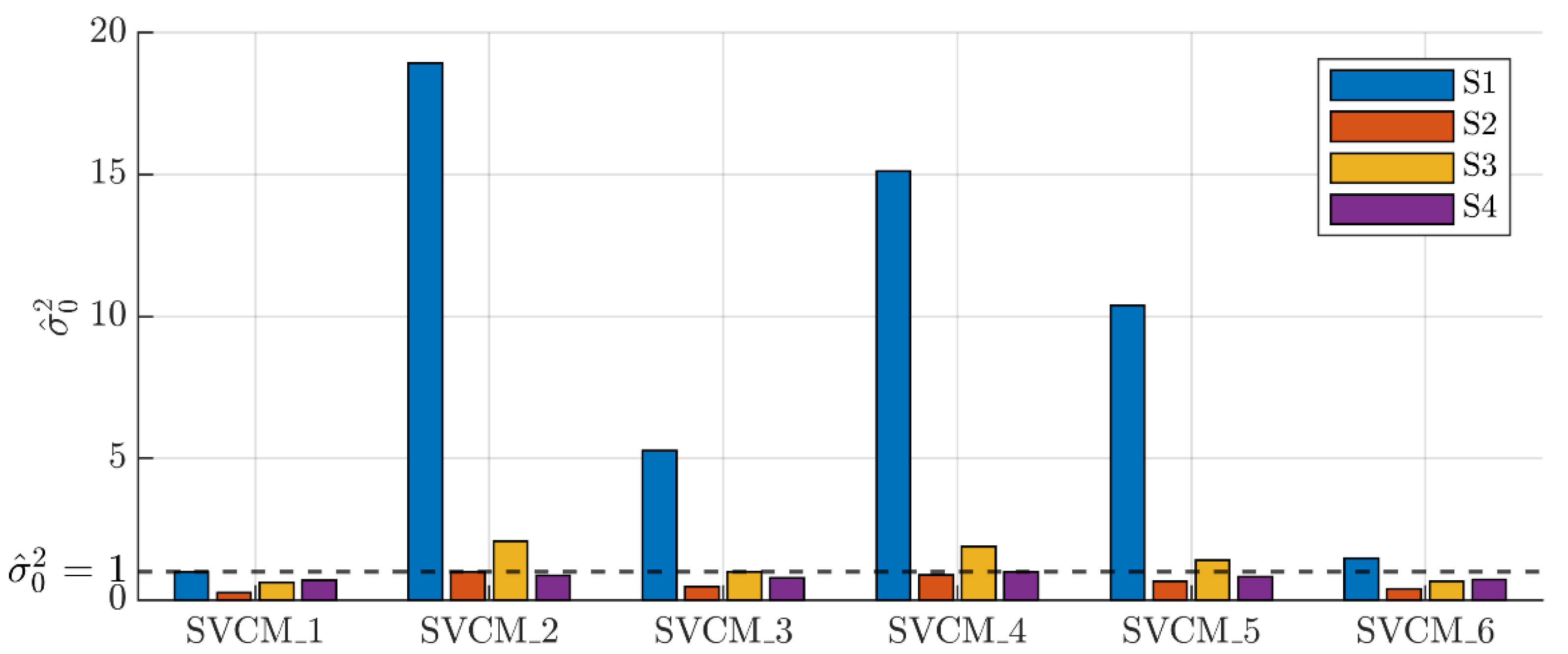
It should be noted that these six SVCMs represent a selection and were justified below. The standard deviations of the non-correlating errors were gradually adjusted so that the first evaluation criterion could be accepted. Figure 6 shows that for each of the four TLS station points (S1-S4) it was necessary to modify the standard deviations of the non-correlating errors in order to prevent rejecting the null hypothesis of the global adjustment test. The first four SVCMs were chosen so that they led to an exact match of the two variance factors at one TLS station point. The values of σ ^ 0 2 for S1 at SVCM_2-5 were strikingly high and could be explained by the increasing influence of the variances and covariances in the SVCM at shorter distances. According to Equations (9) and (10), some variances of functional-correlating errors had the squared distance as the denominator. Thus, adopting the constant variances of the elementary errors, the values in the SVCM were larger at short distances compared with longer ones. Hence, for TLS station point S1, the relative contribution of functional correlating errors and non-correlating errors had to be adapted so that the evaluation criterion one was fulfilled. The standard deviations of the non-correlating errors were set in SVCM_5 so that σ ^ 0 2 approached one as close as possible simultaneously for the three TLS station points S2-S4. This joint consideration of σ ^ 0 2 was extended to all four stations when fixing SVCM_6 and was the attempt to specify a consensus dataset which gave an acceptable result for all four TLS station points in terms of the evaluation criterion 1. Finally, it must be mentioned that different constellations of the non-correlating errors were possible and similar results as shown in Figure 6 were obtained. Since the parameters always had to be adjusted step by step, this required a lot of computing effort and time. Therefore, this work was limited to the six SVCMs specified.
Table 4 serves to compare the three different stochastic models (I, D, SVCM) on the basis of the comparison criterion 1. Obviously, the identity matrix used as cofactor matrix was a too pessimistic assumption for the stochastic model. In general, it could be seen that the a posteriori variance factors σ ^ 0 2 obtained for the identity matrix as well as for the diagonal matrix were always smaller than the a posteriori variance factor of the corresponding SVCM. Since only the main diagonal was populated in the stochastic models of the identity matrix and the diagonal matrix, it could be assumed that the increase in σ ^ 0 2 was due to the covariances.
In three out of four cases, where the ideal SVCM was found for each station point, the difference between a fully populated matrix and a diagonal matrix was small (less than 0.2), which showed that the diagonal matrix could be accepted as a pessimistic assumption for the stochastic model. However, the most dominant difference occurred at SVCM_2 for S2 where it can be concluded that considering the covariances significantly improved the stochastic model.
For approach (a) the standard deviations of the three coordinates of a control point were identical, which was due to the used functional model (refer to Section 2.1). Beyond investigating the impact of the three types of stochastic models, the influence on the estimated parameter’s precision due to a station-wise adapted stochastic model (SVCM_1 to SVCM_4, respectively) and an overarching adapted stochastic model (SVCM_6) was analyzed.
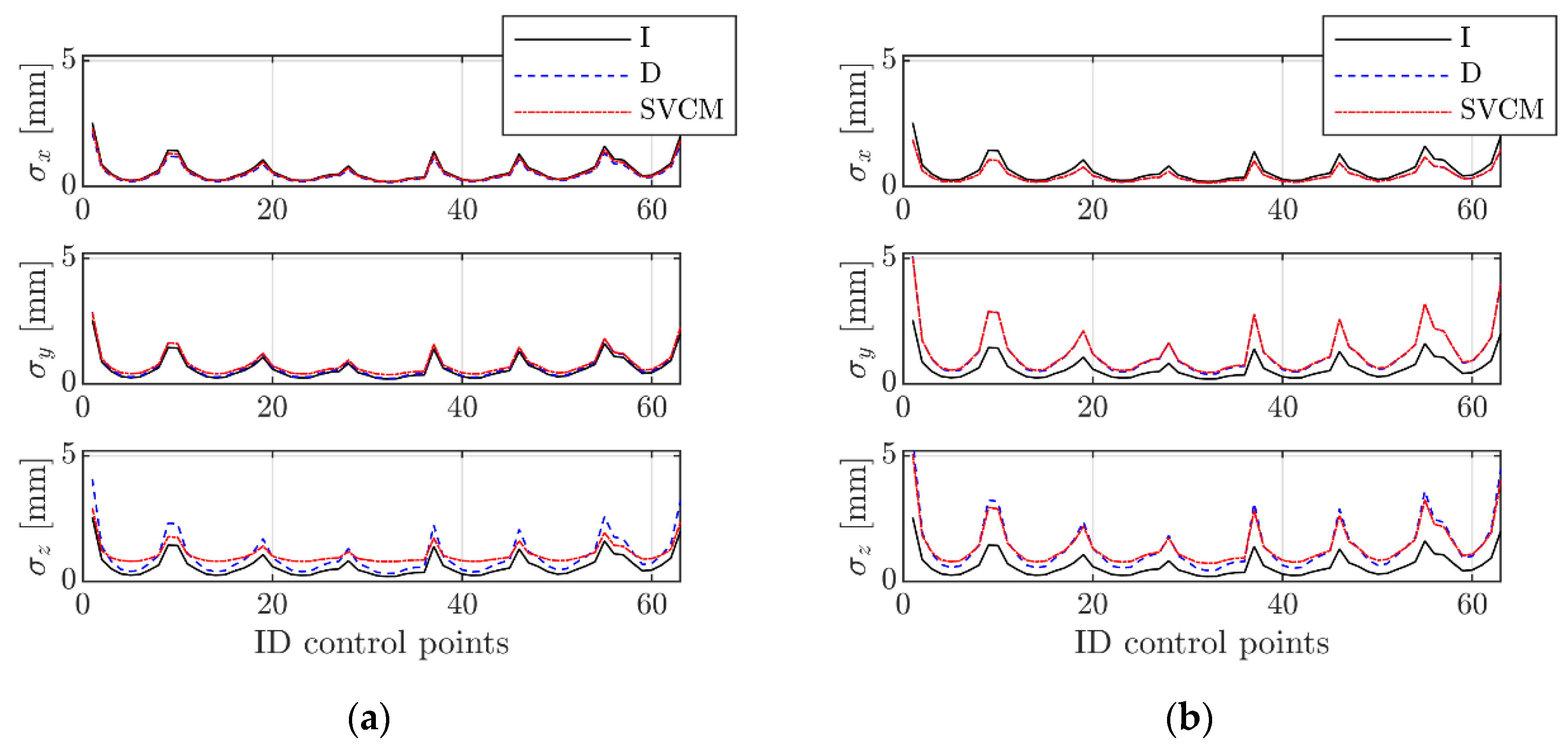
The stochastic influence of SVCM_3 and SVCM_6 for S3 are shown representatively for all TLS station points based on the a posteriori standard deviations (see Section 3.2) in Figure 7a,b. For all TLS station points, the behavior of the a posteriori precision was similar.
The comparison of the precision measures obtained for the station-wise adapted and overarching-wise adapted stochastic models showed that for each station the precision of the estimated parameters decayed for the latter one. This effect occurred independently from σ ^ 0 2   lying over or below one and emphasized the added value of applying a comprehensive stochastic model. This conclusion complied with the conclusions drawn from the simulation study in Section 2.3.
Noticeable in Figure 7 are the peaks that occurred, which are also seen in the following Figures with regard to precision measures. The main reason for their occurrence was the control points’ geometric configuration. The peaks correspond to control points being located at the surface’s corners. Thus, their appearance was a configuration issue, reflecting that parameter estimation results at the borders were less precise than the ones in the middle.
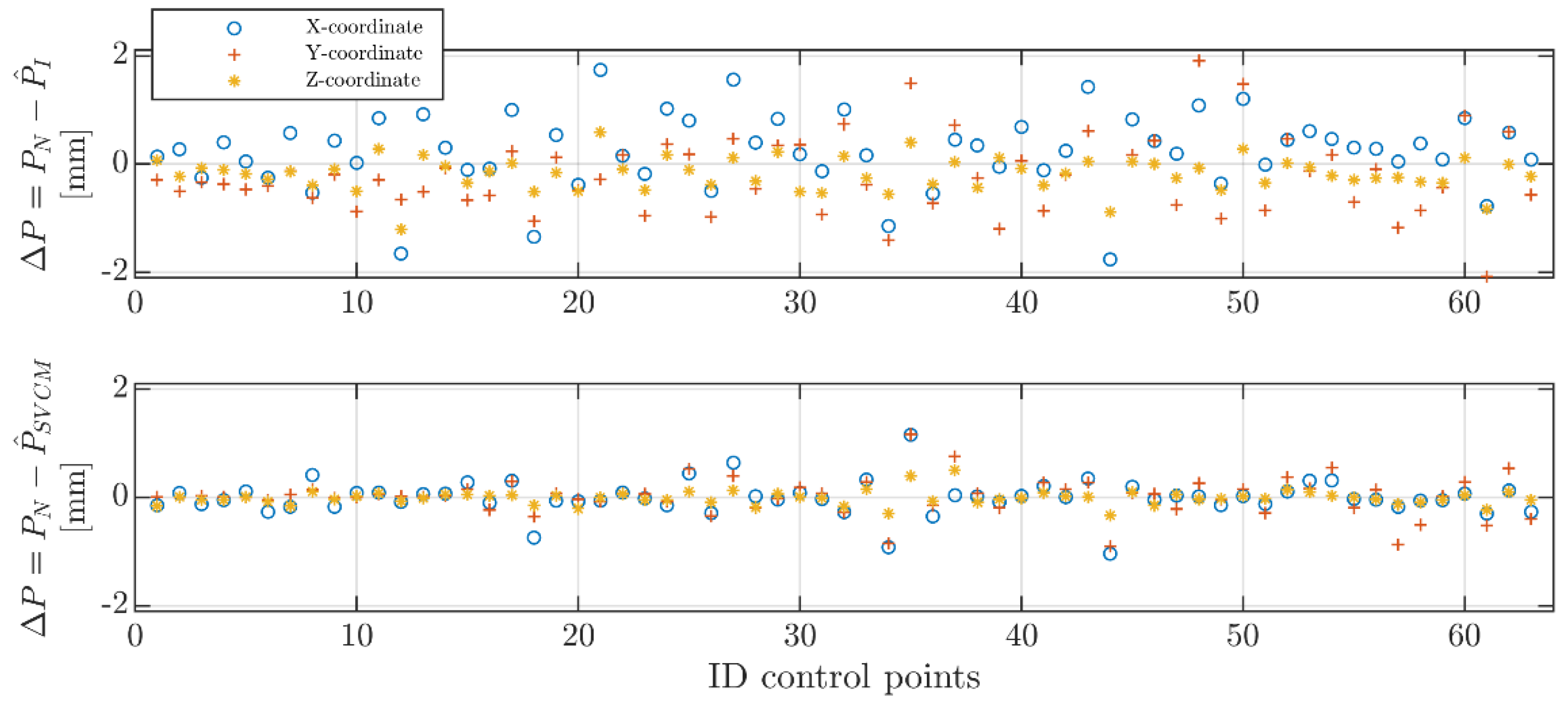
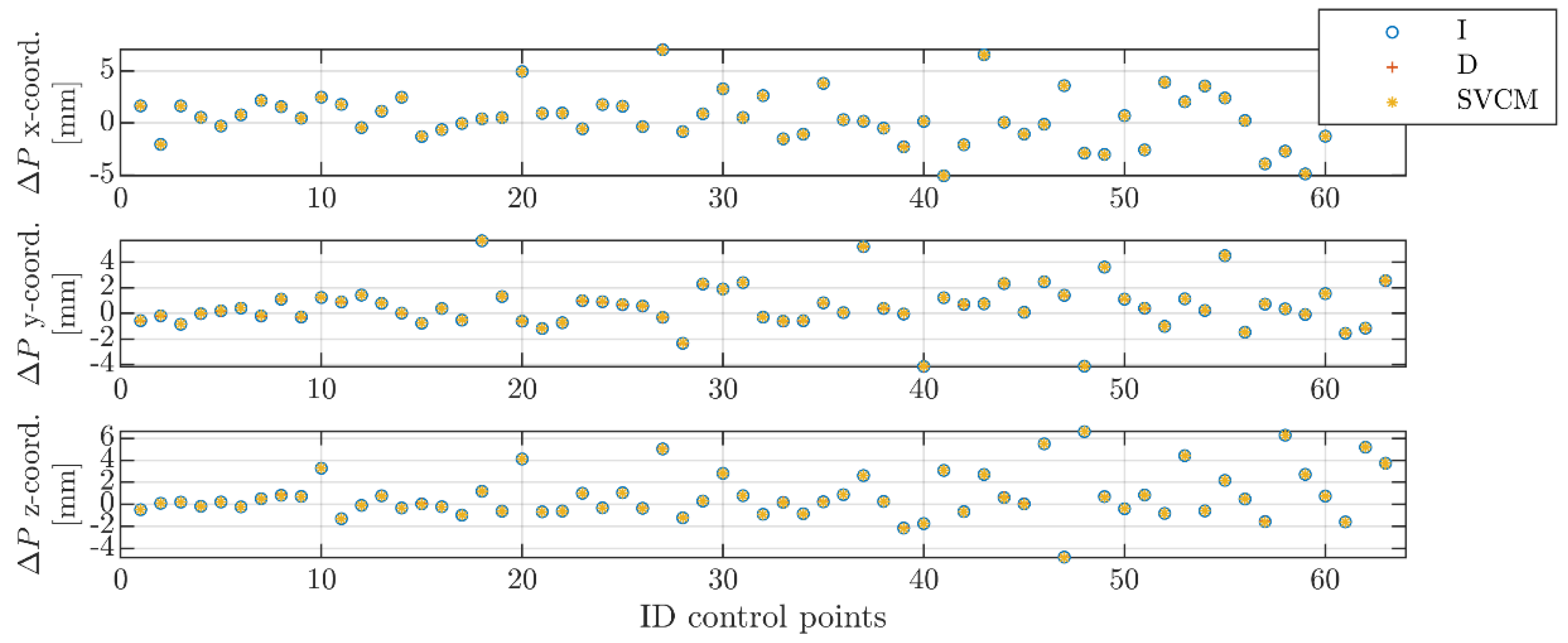
The evaluation according to the third evaluation criterion implied analyzing the differences of the nominal control points and estimated ones. Figure 8 shows an example of differences between the nominal and estimated control points obtained for the three stochastic models (I, D, SVCM) in case of S1 and using SVCM_1. For all three coordinate directions, the differences between estimated control points of the three stochastic models (I, D, SVCM) (see Figure 8) behaved approximately the same and lied in the range of a few tenths of millimeters. With regard to the nominal control points, differences were in the range of a few millimeters. This behavior could also be shown for all other TLS station points and was not presented further in this paper. It could be concluded from Figure 8 that the choice of a particular stochastic model among the three ones had no significant functional influence on the estimated control points.
In this section, the investigation was on the influence of the variance of the non-correlating elementary errors on the functional as well as on the stochastic components of the B-spline approximation results (influence of the first summands in Equation (4)). It turned out that in the varied range, these variances had practically no impact on the estimated control points. On the other hand, their estimated precision was certainly influenced by the chosen variance level of the non-correlating errors. Selecting an adequate variance level for these errors was mandatory to increase the estimation precision. This followed from the comparison of results obtained with station-wise and overarching-wise adapted stochastic models.

4.2. Investigation of Individual Errors and Their Impact

Changing the variance level of an elementary error led to different values of the points’ errors of position and as well as to different values of the covariances. The aim of this section was to investigate how the values chosen for each individual parameter influenced the SVCM and, finally, the estimation results. Additionally, a better understanding of the TLS model presented in Section 2.2 and its influences was pursued.
In the upcoming section, the individual impact of several errors’ variances on the estimated surface were analyze. Three functional correlating errors were selected based on their influence on the SVCM. Each one led to different effects on the estimated surface along the three coordinate axes defined as explained in Section 3.1. An increase in the variance of the chosen CPs led to a decrease in the surface quality only in the specific direction. To be more specific, the precision of estimated control points would be lower in some directions if some of these errors dominated. Not only did these errors have an impact on the main diagonal of the SVCM, but also on the covariances. This was why they were interesting in contrast to non-correlating errors that only filled up the main diagonal. Results were evaluated using the same three criteria from Section 3.2. Additionally, spatial correlations were extracted out of the SVCM and analyzed for each of the functional correlating errors.
The chosen CPs were the zero point error x 10 and its influence along the x-direction, the vertical index error x 4 along the z-direction and horizontal beam offset x 1 n mainly along the y-direction. At a closer look at Equations (6)–(8), it was seen that after linearization, the influencing coefficients that filled the F matrix (see Equation (10)) were one for the corresponding quantities in the case of x 10 (on distances) and x 4 (on vertical angles). Regarding   x 1 n , the influencing coefficients were more complex and had an impact on the horizontal and vertical angles as well as on their covariances. For a relevant inspection, only the selected parameters of the functional correlating group were assigned a value, while all other errors of the same group were set to zero. It was, however, impossible to study the functional correlating errors isolated from the non-correlating errors. This was due to the matrix’ nature, which became singular when solely considering functional correlating errors and did not have an inverse. Therefore, the optimal set of non-correlating errors (SVCM_6 see Table 3) obtained from Section 4.1 were kept constant for all calculated SVCMs, and only the variances of the aforementioned three functional correlating errors were varied.

4.2.1. Zero Point Error x 10

The zero point error x 10 only affected the distances. This became clear by looking at the SVCM in observation space where the range noise σ R 2 was simply added to σ x 10 2 . Apart from the main diagonal, the resulting covariances after matrix multiplication were given by σ x 10 2 .
The variance of x 10 was changed from realistic values in the range of tens of µm up to tens of millimeters. The chosen values were based on the starting value of 0.06 mm and then multiplied with a factor (see Table 5).
According to the first evaluation criterion, σ ^ 0 2 of the fully populated matrix was analyzed after the surface was estimated with each of the SVCMs from Table 5. Within this variance level, σ ^ 0 2   did not change significantly, but remained as presented in Table 4 at SVCM_6 for all station points. Differences were only noticeable after six digits.
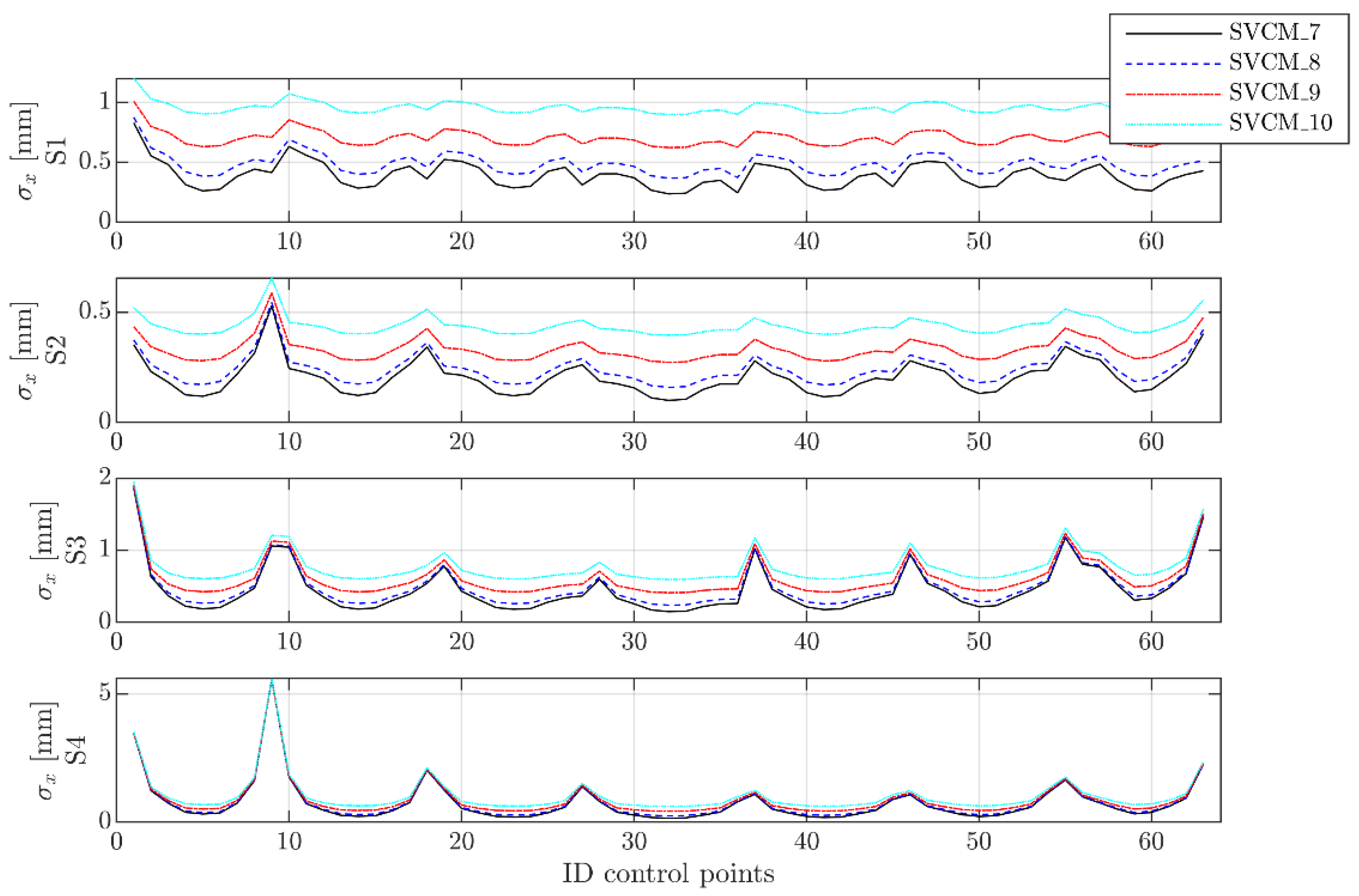
Judging by the second criterion, the accuracy of the estimated control points changed for each station point and for each SVCM. As in the previous case, precisions were lower at close range. This was especially noticeable at S1 and S2 (see Figure 9). In the case of S2, the precisions were slightly lower than at S1; a fact that could be explained with the slightly better transformation of S2 in the LT coordinate system (0.2 mm average residuals for S2, 0.4 mm average residuals for S1). For the other station points (S3 and S4), the graphics follow a similar profile at closer inspection.
Striking in Figure 9 are the increased values of the peaks from S1 to S4. This was mainly due to the configuration of the measurements, leading to corresponding entries in the design matrix A . At the edges of the test specimen, the observations were sparser and, thus, control points in that area were estimated with a lower precision for the different station points. A reference based on network measurements can be found in [33]. Related to the B-spline estimation, a similar behavior of the precision measures was provided in [15,21].
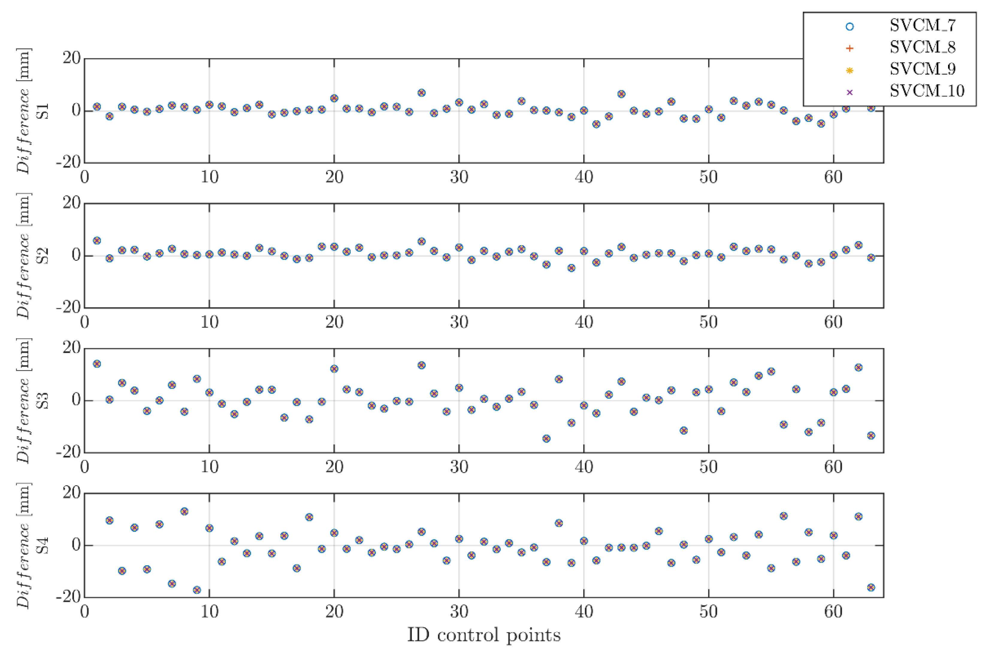
Finally, the third criterion implied analyzing the differences of the nominal control points and estimated ones. Because this error only affected the x coordinates, only this dimension was presented for the comparison. For each station point, all versions of SVCMs were used for the estimation. Results are presented in Figure 10.
As can be seen, there were no noticeable differences in the x-direction for the matrices SVCM_7 to SVCM_10.
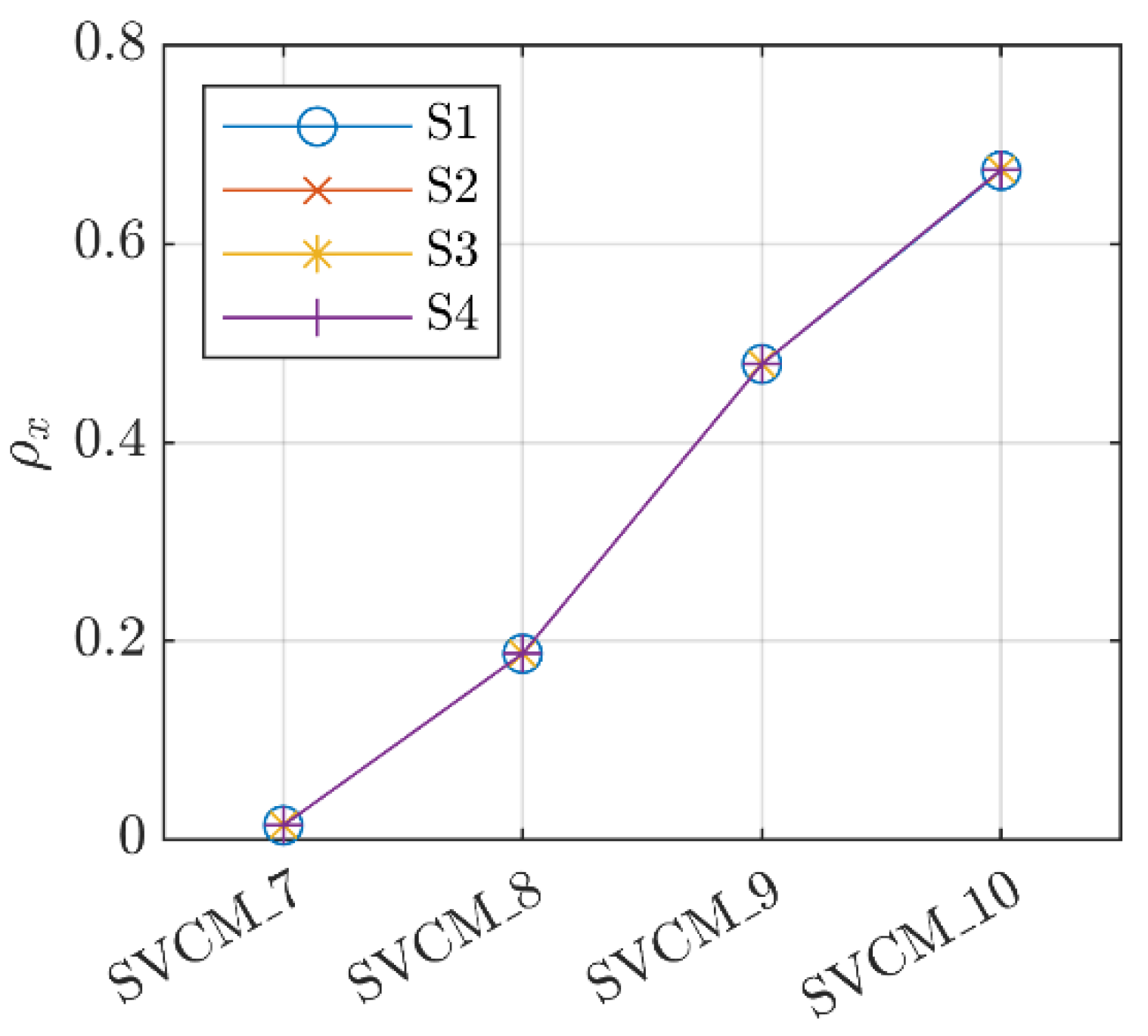
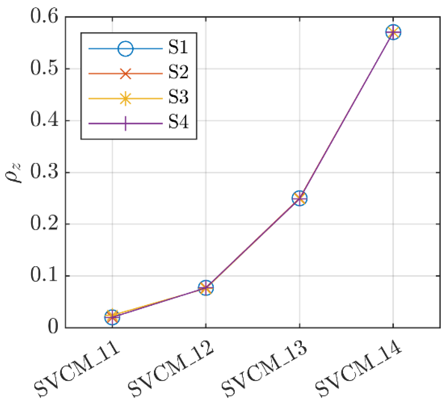
Another aspect that was studied was the average spatial correlation coefficient between the points in the point cloud. A correlation matrix was computed based on different versions of the SVCM and afterwards, coefficients were extracted for all elements along one axis (here x). Figure 11 shows how the spatial correlation coefficient increased in all four versions of the SVCM and for all station points with an increasing variance of x 10 . If this was analyzed together with the numerical value for the range noise variance σ R 2 , then the correlation coefficient ρ x was exactly 0.5 when σ R 2 = σ x 10 2 . When this threshold was exceeded, σ x 10 2 started to dominate the variances.
Comparable results were found for the vertical index error x 4 . The corresponding results and figures can be found in Appendix A.

4.2.2. Horizontal Beam Offset x 1 n

In contrast to other functional correlating errors, x 1 n differently influenced horizontal and vertical angles, as well as the covariances between these. In all cases, the influence on the SVCMs was proportional with the scanning distance. As seen in Equation (10), the influencing factors were the range R as the denominator, meaning that at close ranges the same variance had a higher impact than at longer ranges.
Further on, the standard deviation of the horizontal beam offset x 1 n was scaled starting from realistic values of 0.14 mm up to 1.12 mm (Table 6).
As in the previous cases, the global quality indicator σ ^ 0 2 did not change.
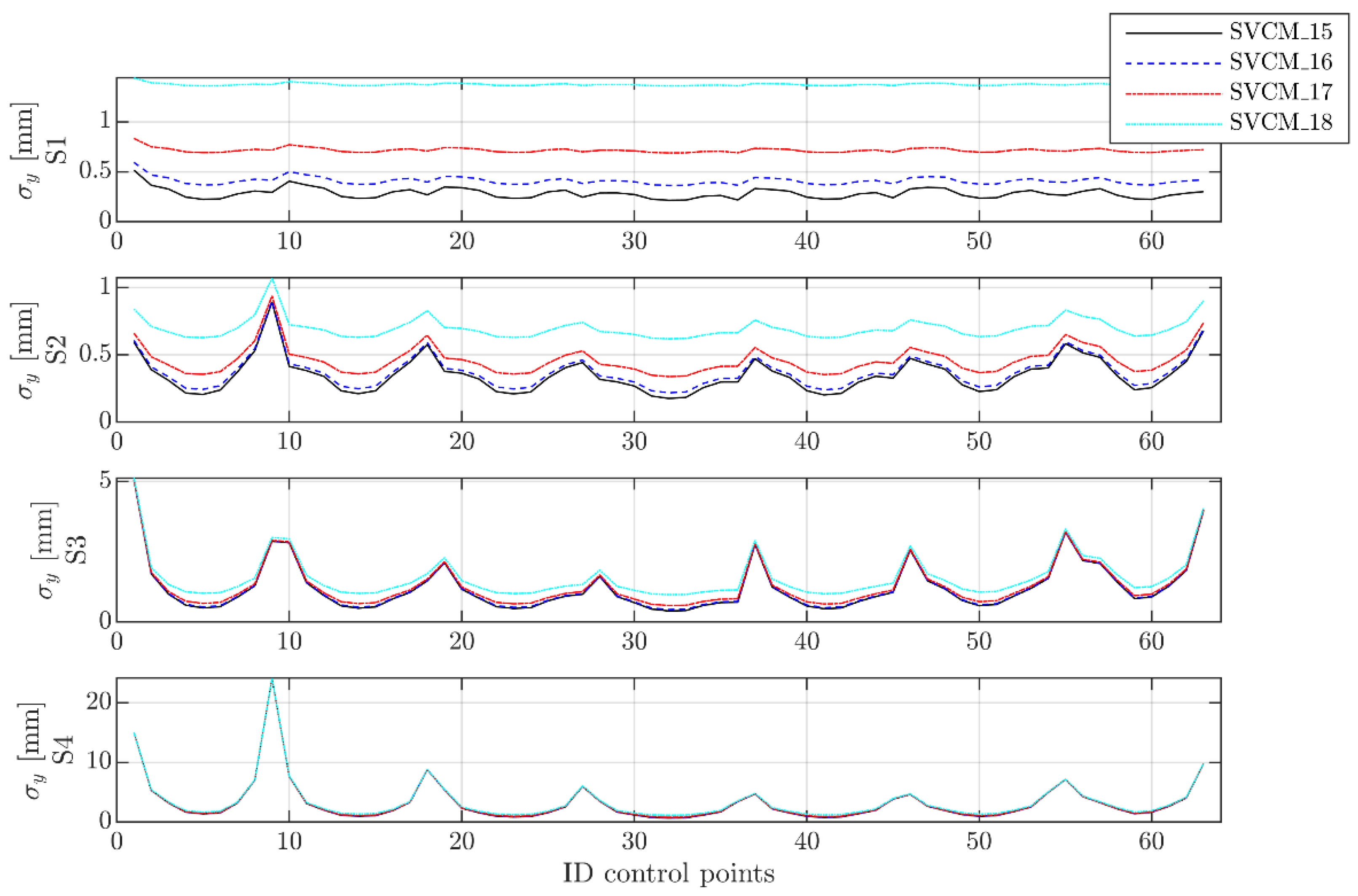
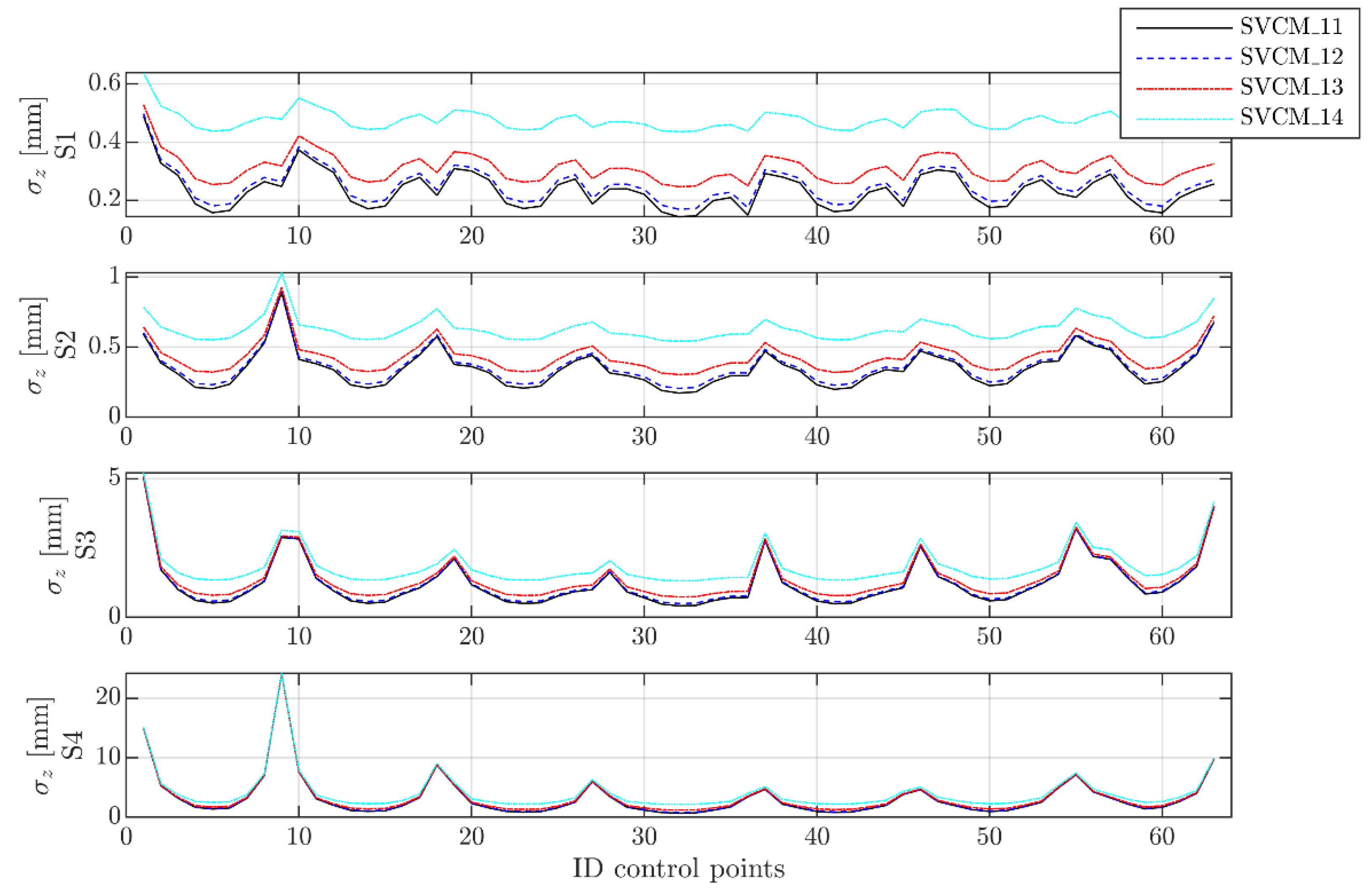
Considering the second criterion, accuracies of the estimated control points were better at close range for reduced variance levels. This was especially noticeable at the first two station points (see Figure 12). The small differences that occurred between S1 and S2 were explainable by the better transformation residuals of S2 in the LT system. The estimation with the best precisions was obtained with SVCM_15 in this case where the variance level was the one determined by the TLS calibration. When compared with the precisions of the estimated control points for the other two individual errors, it was seen that at a close range (S1), the precisions remained approximately constant at the same level. All other station points showed a similar spike profile (saw profile), indicating that the position of control points played an important role especially at longer ranges.
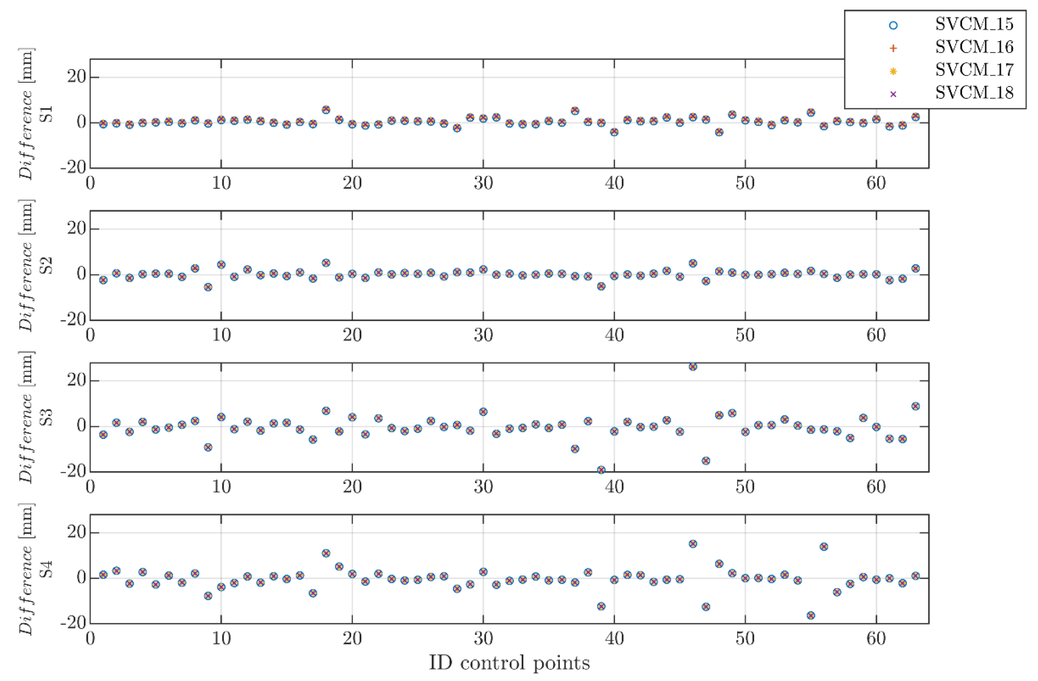
The differences of the nominal control points and the estimated ones in y-direction were the same in three out of four cases for all versions of the SVCM (Figure 13). Only in the case of S1, differences in a few tenths of mm occurred and this fact was directly related with the above-mentioned denominator. Just to give an example, the same value of σ x 1 n 2 was denominated at S1 with 6² m whilst at S4 with 44² m; therefore, having a considerable effect at close ranges.
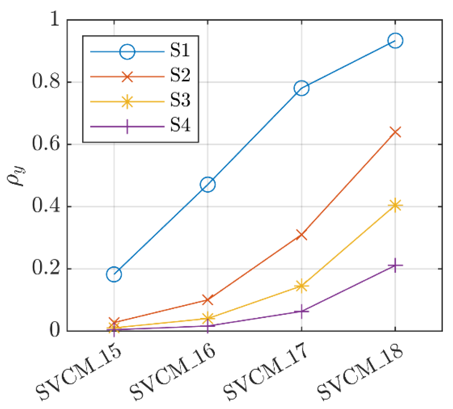
When inspecting the spatial correlations, it was obvious that these were different for all versions of the SVCM as well as for each station point (Figure 14). Firstly, this showed the more complex impact of the horizontal beam offset on the SVCM and pointed out that the scanning configuration (distance from scanner to object) together with the variance level was decisive for the spatial correlations. The reason for this was, as explained before, a normalization by R² of the covariances that affected the y-direction.

5. Conclusions

Within this contribution, a systematic approach of establishing SVCMs for modelling point clouds by B-spline free-form elements was presented. Motivated by simulated results, a stochastic model was defined using the elementary error theory and applied for TLS high-end panoramic scanners. Striving for similar results for real measurements, laboratory measurement on a small-scale B-spline reference object were conducted. Point clouds originating from four TLS station points were used to estimate B-spline surfaces and, furthermore, to evaluate the impact of the used SVCM on the surface’s parameters as well as their precision. Three criteria were used to evaluate this impact.
Firstly, the a posteriori variance factor, a global measure of precision, aided to establish appropriate variances for the non-correlating errors corresponding to the noise of the three polar observations. Neglecting the correlations, by using the identity or the diagonal matrix as a stochastic model led to an overoptimistic estimation of the precision (see Table 4). A station-wise adaption of the stochastic model could dramatically decrease the precision of the estimations from stations with different measurement conditions (see Table 4).
Secondly, the a posteriori precision of the estimated control points was assessed by using the identity matrix, a diagonal matrix and a fully populated SVCM. A stochastic model adapted as well as possible to the measurement situation led to results with a smallest distortion and of the highest precision. This was shown based on a simulation (see Figure 1) as well as through a dedicated station-wise adaption of the variances of the non-correlating elementary errors (see Figure 7). Using fully populated SVCMs led to negligible differences of the estimated precision compared to the other two structures of stochastic models. However, noticeable differences between the precisions occurred when using the station-wise and overarching-wise adapted SVCMs. These emphasized the importance of setting proper variance levels for the non-correlating errors when aiming the highest precision in parameter estimation.
Thirdly, reference values of the known control points were used to examine coordinate-wise differences between nominal and estimated control points. This evaluated the correctness of the functional part of the estimation results. No significant difference between the estimation’s biases could be observed when an approximation with an identity matrix, diagonal matrix or a fully populated SVCM (see Figure 8) was performed.
Additionally, individual functional correlating elementary errors (zero point error, vertical index error and horizontal beam offset) were analyzed. It turned out that their increasing variances led to a lower precision of the estimated control points. Furthermore, the differences between the precision resulting from different SVCMs decreased with an increased distance to the measuring object (see Figure 9, Figure 12 and Figure A1). Moreover, no significant bias could be found in the differences of the estimated control points with the nominal control points. In addition, the differences between the biases obtained with the estimated control points using different SVCMs were not significant (see Figure 10 and Figure 13). The higher the variance of the functional correlating elementary errors, the higher the average correlation between the measurements. The increase was more pronounced for station points closer to the measuring object (see Figure 11, Figure 14 and Figure A2).
As regards future research, the same workflow will be applied for objects of a tenth of an m level and outdoor scans in order to identify contributions of further elementary errors to the uncertainty budget. It is also planned to include the stochastic correlating errors such as environment influences and surface properties.

Author Contributions

Conceptualization, J.R., G.K., C.H., V.S. and H.N.; methodology, G.K.; software, J.R., G.K. and C.H.; validation, C.H., V.S. and H.N.; investigation, J.R., G.K. and C.H.; resources, J.R., G.K., C.H., V.S. and H.N.; data curation, G.K.; writing—original draft preparation, J.R. and G.K.; writing—review and editing, J.R., G.K., C.H., V.S. and H.N.; visualization, J.R.; supervision, V.S. and H.N.; project administration, V.S. and H.N.; funding acquisition, V.S. and H.N. All authors have read and agreed to the published version of the manuscript.

Funding

This research was partly funded by the DFG (German Research Foundation), SCHW 838/7-3 within the project IMKAD II “Integrated space-time modeling based on correlated measurements for the determination of survey configurations and the description of deformation processes”. The project was also an associated project (AP 07) with the Cluster of Excellence Integrative Computational Design and Construction for Architecture (IntCDC) partially supported by the DFG under Germany’s Excellence Strategy—EXC 2120/1—390831618. The other funding party of IMKAD II (I3869) was the Austrian Science Fund (FWF). The authors express their gratitude to the DFG and the FWF for funding this project.

Institutional Review Board Statement

Not applicable.

Informed Consent Statement

Not applicable.

Data Availability Statement

The data presented in this study are available on request from the corresponding author. The data are not publicly available due to large data size.

Acknowledgments

We cordially thank the Society for Calibration of Geodetic Devices (SCGD) and the Institute of Engineering Geodesy research associates Laura Balangé and Urs Basalla for providing calibration data of the Leica HDS 7000. Data were gathered within the COLLECTOR project.

Conflicts of Interest

The authors declare no conflict of interest.

Appendix A. Vertical Index Error x 4

The variance of the vertical index error x 4 was chosen due to its influence on the variances and covariances of vertical angles and implicitly the z coordinate. Within the SVCM, it had the exact effect on vertical angles as x 10 has on the distances. In the observation space, the vertical angle noise σ θ 2 was simply added to σ x 4 2 . Apart from the main diagonal, the resulting covariances after matrix multiplication were given by σ x 4 2 . Values of the variance were changed starting from realistic values under 1 mgon up to a few mgon. The chosen values were based on the starting value of 0.45 mgon and then multiplied with a factor (see Table A1).
Table A1. Versions of SVCM with different standard deviations for vertical index error x 4 .
SVCM_11SVCM_12SVCM_13SVCM_14
σ x 4 (mgon)0.450.901.793.58
Within this variance level, σ ^ 0 2   did not change, but remained as presented in Table 4 at SVCM_6 for all station points. This was also reflected by means of the differences between the nominal control points and estimated ones. Only the differences along z were inspected for each station point and all versions of the SVCM. Here, the differences between the estimated control points in z-direction while using the SVCM_11 to SVCM_14 were not distinguishable.
Looking at the second criterion, the behavior was comparable to the zero point error. The precision of the estimated control points was low at a close range and only small differences were noticeable for an increasing variance level (see Figure A1). With an increasing distance, precisions decreased and followed the same pattern.
Figure A1. Precisions of the estimated control points in z-direction.
Remotesensing 13 03124 g0a1
Similar to the spatial correlation analysis determined before, coefficients were extracted for all elements along the z-axis. In Figure A2, the spatial correlation coefficient increased in all four versions of the SVCM and for all station points with an increasing variance of x 4 . The trend was the same as in the zero point error, but the equivalent non-correlating error in this case was σ θ the vertical angle noise.
Figure A2. Average correlation along z-direction for different SVCMs for x 4 .
Remotesensing 13 03124 g0a2

References

  1. Wujanz, D. Terrestrial Laser Scanning for Geodetic Deformation Monitoring. Ph.D. Thesis, Technische Universität Berlin, Berlin, Germany, 2016. [Google Scholar] [CrossRef]
  2. Kuhlmann, H.; Holst, C. Flächenhafte Abtastung mit Laserscanning: Messtechnik, flächenhafte Modellierungen und aktuelle Entwicklungen im Bereich des terrestrischen Laserscannings. In Ingenieurgeodäsie; Schwarz, W., Ed.; Springer: Berlin/Heidelberg, Germany, 2017; pp. 167–212. ISBN 978-3-662-47187-6. [Google Scholar] [CrossRef]
  3. Mukupa, W.; Roberts, G.W.; Hancock, C.M.; Al-Manasir, K. A review of the use of terrestrial laser scanning application for change detection and deformation monitoring of structures. Surv. Rev. 2016, 49, 99–116. [Google Scholar] [CrossRef]
  4. Harmening, C.; Neuner, H. Detecting rigid body movements from TLS-based areal deformation measurements. In Proceedings of the 78th FIG Working Week 2016, Christchurch, New Zealand, 2–6 May 2016. [Google Scholar]
  5. Harmening, C.; Neuner, H. A constraint-based parameterization technique for B-spline surfaces. J. Appl. Geod. 2015, 9, 143–161. [Google Scholar] [CrossRef]
  6. Schmitt, C.; Neuner, H. Knot estimation on B-Spline curves. Osterr. Z. Für Vermess. Geoinf. 2015, 103, 188–197. [Google Scholar]
  7. Gálvez, A.; Iglesias, A.; Avila, A.; Otero, C.; Arias, R.; Manchado, C. Elitist clonal selection algorithm for optimal choice of free knots in B-spline data fitting. Appl. Soft Comput. 2015, 26, 90–106. [Google Scholar] [CrossRef]
  8. Bureick, J.; Alkhatib, H.; Neumann, I. Fast converging elitist genetic algorithm for knot adjustment in B-spline curve approximation. J. Appl. Geod. 2019, 13, 317–328. [Google Scholar] [CrossRef]
  9. Harmening, C.; Neuner, H. Choosing the optimal number of B-spline control points (Part 2: Approximation of surfaces and applications). J. Appl. Geod. 2017, 11, 43–52. [Google Scholar] [CrossRef]
  10. Hagen, G. Grundzüge der Wahrscheinlichkeits-Rechnung; Ed. Dümmler: Berlin, Germany, 1867. [Google Scholar]
  11. Geheimen-Rath; Bessel, R. Untersuchungen über die Wahrscheinlichkeit der Beobachtungsfehler. Astron. Nachr. 1838, 15, 369–404. [Google Scholar] [CrossRef] [Green Version]
  12. Pelzer, H. Grundlagen der mathematischen Statistik und der Ausgleichungsrechnung. In Geodätische Netze in. Landes-und Ingenieurvermessung II; Konrad Wittwer Verl: Stuttgart, Germany, 1985. [Google Scholar]
  13. Koch, K.-R. Determining uncertainties of correlated measurements by Monte Carlo simulations applied to laserscanning. J. Appl. Geodesy 2008, 2, 139–147. [Google Scholar] [CrossRef]
  14. Wujanz, D.; Burger, M.; Mettenleiter, M.; Neitzel, F. An intensity-based stochastic model for terrestrial laser scanners. ISPRS J. Photogramm. Remote Sens. 2017, 125, 146–155. [Google Scholar] [CrossRef]
  15. Kauker, S.; Harmening, C.; Neuner, H.; Schwieger, V. Modellierung und Auswirkung von Korrelationen bei der Schätzung von Deformationsparametern beim terrestrischen Laserscanning. In Beiträge zum 18. Internationalen Ingenieurvermessungskurs in Graz; Lienhart, W., Ed.; Wichmann Verlag: Berlin, Germany, 2017; pp. 321–336. ISBN 978-3-87907-630-7. [Google Scholar]
  16. Piegl, L.; Tiller, W. The NURBS Book; Springer: Berlin/Heidelberg, Germany, 1997; ISBN 978-3-540-61545-3. [Google Scholar] [CrossRef]
  17. Bureick, J.; Neuner, H.; Harmening, C.; Neumann, I. Curve and Surface Approximation of 3D Point Clouds. Allg. Vermess. Nachr. 2016, 123, 315–327. [Google Scholar]
  18. Cox, M.G. The Numerical Evaluation of B-Splines. IMA J. Appl. Math. 1972, 10, 134–149. [Google Scholar] [CrossRef]
  19. de Boor, C. On calculating with B-splines. J. Approx. Theory 1972, 6, 50–62. [Google Scholar] [CrossRef] [Green Version]
  20. Bureick, J.; Alkhatib, H.; Neumann, I. Robust spatial approximation of laser scanner point clouds by means of free-form curve approaches in deformation analysis. J. Appl. Geod. 2016, 10, 27–35. [Google Scholar] [CrossRef]
  21. Harmening, C.; Neuner, H. Choosing the Optimal Number of B-spline Control Points (Part 1: Methodology and Approximation of Curves). J. Appl. Geod. 2016, 10, 139–157. [Google Scholar] [CrossRef]
  22. Harmening, C. Spatio-Temporal Deformation Analysis Using Enhanced B-Spline Models of Laser Scanning Point Clouds. Ph.D. Thesis, TU Wien, Wien, Austria, 2020. [Google Scholar] [CrossRef]
  23. Schwieger, V. Ein Elementarfehlermodell Für GPS-Überwachungsmessungen Konstruktion und Bedeutung Interepochaler Korrelationen; Fachrichtung Vermessungswesen der University: Hannover, Germany, 1999; ISBN 0174-1454. [Google Scholar]
  24. Kauker, S.; Schwieger, V. A synthetic covariance matrix for monitoring by terrestrial laser scanning. J. Appl. Geod. 2017, 11. [Google Scholar] [CrossRef]
  25. Kerekes, G.; Schwieger, V. Elementary Error Model Applied to Terrestrial Laser Scanning Measurements: Study Case Arch Dam Kops. Mathematics 2020, 8, 593. [Google Scholar] [CrossRef]
  26. Kerekes, G.; Schwieger, V. Determining Variance-Covariance Matrices for Terrestrial Laser Scans: A Case Study of the Arch Dam Kops. In Contributions to International Conferences on Engineering Surveying; Kopáčik, A., Kyrinovič, P., Erdélyi, J., Paar, R., Marendić, A., Eds.; Springer International Publishing: Berlin/Heidelberg, Germany, 2021; pp. 57–68. ISBN 978-3-030-51952-0. [Google Scholar] [CrossRef]
  27. Muralikrishnan, B.; Ferrucci, M.; Sawyer, D.; Gerner, G.; Lee, V.; Blackburn, C.; Phillips, S.; Petrov, P.; Yakovlev, Y.; Astrelin, A.; et al. Volumetric performance evaluation of a laser scanner based on geometric error model. Precis. Eng. 2015, 40, 139–150. [Google Scholar] [CrossRef]
  28. Medić, T.; Kuhlmann, H.; Holst, C. Sensitivity Analysis and Minimal Measurement Geometry for the Target-Based Calibration of High-End Panoramic Terrestrial Laser Scanners. Remote Sens. 2019, 11, 1519. [Google Scholar] [CrossRef] [Green Version]
  29. Medić, T.; Kuhlmann, H.; Holst, C. A priori vs. In-situ Terrestrial Laser Scanner Calibration in the Context of the Instability of Calibration Parameters. In Contributions to International Conferences on Engineering Surveying; Kopáčik, A., Kyrinovič, P., Erdélyi, J., Paar, R., Marendić, A., Eds.; Springer International Publishing: Berlin/Heidelberg, Germany, 2021; pp. 128–141. ISBN 978-3-030-51952-0. [Google Scholar] [CrossRef]
  30. Medić, T. Efficient Calibration Strategies for Panoramic Terrestrial Laser Scanners. Ph.D. Thesis, Rheinische Friedrich-Wilhelms-Universität Bonn, Bonn, Germany, 2021. [Google Scholar]
  31. Alkhatib, H.; Neumann, I.; Kutterer, H. Uncertainty modeling of random and systematic errors by means of Monte Carlo and fuzzy techniques. J. Appl. Geod. 2009, 3, 67–79. [Google Scholar] [CrossRef] [Green Version]
  32. ISO 17123-9:2018-12 Optics and Optical Instruments—Field Procedures for Testing Geodetic and Surveying Instruments—Part 9: Terrestrial Laser Scanners; ISO: Geneva, Switzerland, 2018.
  33. Niemeier, W. Ausgleichungsrechnung: Statistische Auswertemethoden, 2nd ed.; de Gruyter, W., Ed.; Amazon: Berlin, Germany, 2008; ISBN 978-3-11-019055-7. [Google Scholar]
  34. Holst, C.; Medić, T.; Blome, M.; Kuhlmann, H. TLS-Kalibrierung: In-situ und/oder a priori? In Terrestrisches Laserscanning 2019 (TLS 2019): Beiträge zum 184. DVW-Seminar am 2. und 3. Dezember 2019 in Fulda; DVW Gesellschaft für Geodäsie, Geoinformation und Landmanagement, Ed.; Wißner-Verlag: Augsburg, Germany, 2019; pp. 89–104. ISBN 978-3-95786-231-0. [Google Scholar]
  35. Leica Geosystems AG HDS7000 User Manual. Available online: w3.leica-geosystems.com/downloads123/hds/hds/HDS7000/brochures-datasheet/HDS7000_DAT_de.pdf (accessed on 1 January 2021).
Figure 1. Differences of the positions of the estimated control points with respect to the nominal coordinates P N using different stochastic models (top: identity matrix; bottom: fully populated VCM).
Remotesensing 13 03124 g001
Figure 2. Control points of the B-spline test specimen.
Remotesensing 13 03124 g002
Figure 3. (a) Nominal point cloud stored in CAD coordinate system ( z C A D axis is orthogonal to the x C A D y C A D plane); (b) test specimen of known B-spline form with reference points.
Remotesensing 13 03124 g003
Figure 4. Overview of experiment set-up.
Remotesensing 13 03124 g004
Figure 5. Work flow diagram (blue—scans; green—process; orange—coordinate systems).
Remotesensing 13 03124 g005
Figure 6. Overview of the resulting σ ^ 0 2 for SVCM_1-6 and the four TLS station points.
Remotesensing 13 03124 g006
Figure 7. (a) A posteriori standard deviations of estimated control points (S3 and SVCM_3); (b) a posteriori standard deviations of estimated control points (S3 and SVCM_6).
Remotesensing 13 03124 g007
Figure 8. Difference between nominal and estimated control points for stochastic models (I, D, SVCM) at S1 and SVCM_1.
Remotesensing 13 03124 g008
Figure 9. Precision of the estimated control points in x-direction.
Remotesensing 13 03124 g009
Figure 10. Differences between nominal and estimated control points in x-direction.
Remotesensing 13 03124 g010
Figure 11. Average correlation along x-direction for different SVCMs for x 10 .
Remotesensing 13 03124 g011
Figure 12. Precisions of the estimated control points in y-direction.
Remotesensing 13 03124 g012
Figure 13. Differences between nominal and estimated control points in y-direction.
Remotesensing 13 03124 g013
Figure 14. Average correlation along y-direction for different SVCMs for x 1 n .
Remotesensing 13 03124 g014
Table 1. Parameter of TLS calibration model.
CPTilts/Angular ErrorsCPOffsets/Metric Errors
x 4 Vertical index error x 1 n Horizontal beam offset
x 5 n Horizontal beam tilt x 1 z Vertical beam offset
x 5 z Vertical beam tilt x 2 Horizontal axis offset
x 6 Collimation axis error x 3 Mirror offset
x 7 Horizontal axis error (tilt) x 10 Zero point error
Table 2. Explicit standard deviations for functional-correlating errors.
CPTilts/Angular Errors (mgon)CPOffsets/Metric Errors (mm)
σ x 4 0.45 σ x 1 n 0.14
σ x 5 n 1.79 σ x 1 z 0.22
σ x 5 z 1.60 σ x 2 0.02
σ x 6 0.27 σ x 3 0.13
σ x 7 1.93 σ x 10 0.06
Table 3. Explicit standard deviations for non-correlating errors.
CPSVCM_1SVCM_2SVCM_3SVCM_4SVCM_5SVCM_6
σ λ ( mgon ) 4.20.71.40.81.03.1
σ θ ( mgon ) 4.20.71.40.81.03.1
σ R ( mm ) 0.50.60.50.50.50.5
Table 4. Comparison of   σ ^ 0 2 of different stochastic models (a–c) for the four TLS station points.
σ ^ 0 2 SVCM_1SVCM_2SVCM_3SVCM_4SVCM_5SVCM_6
S1 Σ l l = I 0.21
Σ l l = D 0.881.941.752.051.921.10
Σ l l = S V C M 1.0018.925.2715.1210.391.46
S2 Σ l l = I 0.09
Σ l l = D 0.260.410.360.460.400.27
Σ l l = S V C M 0.271.000.460.890.660.38
S3 Σ l l = I 0.30
Σ l l = D 0.590.960.821.070.910.63
Σ l l = S V C M 0.612.081.001.891.400.65
S4 Σ l l = I 0.27
Σ l l = D 0.680.640.740.820.720.69
Σ l l = S V C M 0.700.870.791.000.820.71
Table 5. Versions of SVCM with different standard deviations for zero point error x 10 .
SVCM_7SVCM_8SVCM_9SVCM_10
σ x 10 (mm)0.060.240.480.72
Table 6. Versions of SVCM with different standard deviations for horizontal beam error x 1 n .
SVCM_15SVCM_16SVCM_17SVCM_18
σ x 1 n (mm)0.140.280.561.12
Publisher’s Note: MDPI stays neutral with regard to jurisdictional claims in published maps and institutional affiliations.

