Article

Investigation on the Relationship between Satellite Air Quality Measurements and Industrial Production by Generalized Additive Modeling

1
School of Management, Hefei University of Technology, Hefei 230009, China
2
Department of Precision Machinery and Precision Instrumentation, University of Science and Technology of China, Hefei 230026, China
*
Author to whom correspondence should be addressed.
Remote Sens. 2021, 13(16), 3137; https://0-doi-org.brum.beds.ac.uk/10.3390/rs13163137
Submission received: 24 May 2021 / Revised: 5 August 2021 / Accepted: 5 August 2021 / Published: 8 August 2021
(This article belongs to the Special Issue Optical and Laser Remote Sensing of Atmospheric Composition)

Abstract

:
The development of the green economy is universally recognized as a solution to natural resource shortages and environmental pollution. When exploring and developing a green economy, it is important to study the relationships between the environment and economic development. As opposed to descriptive and qualitative research without modeling or based on environmental Kuznets curves, quantitative relationships between environmental protection and economic development must be identified for exploration and practice. In this paper, we used the generalized additive model (GAM) regression method to identify relationships between atmospheric pollutants (e.g., NO2, SO2 and CO) from remote sensing and in situ measurements and their driving effectors, including meteorology and economic indicators. Three representative cities in the Anhui province, such as Hefei (technology-based industry), Tongling (resource-based industry) and Huangshan (tourism-based industry), were studied from 2016 to 2020. After eliminating the influence of meteorological factors, the relationship between air quality indexes and industrial production in the target cities was clearly observed. Taking Hefei, for example, when the normalized output of chemical products increases by one unit, the effect on atmospheric NO2 content increases by about 20%. When the normalized output of chemical product increases by one unit, the effect on atmospheric SO2 content increases by about 10%. When chemical and steel product outputs increase by one unit, the effect on atmospheric CO content increases by 25% and 20%, respectively. These results can help different cities predict local economic development trends varying by the changes in air quality and adjust local industrial structure.

1. Introduction

The green economy is a model of sustainable development that is globally recognized to meet challenges posed by increasing shortages of energy and natural resources [1] As an important engine of the world economy, China’s attitude and solutions can greatly contribute to green economic development worldwide [2]. After forty years of industrialization, China has achieved economic success with the costs of natural resources consumption and destruction of the environment [3]. Industrial transformation and upgrades were in urgent demand for China’s economic development [4]. The Chinese government set a target for reaching a carbon peak by 2030 and becoming carbon neutral by 2060 to demonstrate its commitment to the green economy [5]. The process of industrial transformation and upgrades in China provides sufficient data and case studies.
The academic research on this problem can be divided into two approaches. Some prior research has focused on technology that directly improves resource use efficiency and reduces environmental pollution [6]. Other studies have focused on effective management approaches that can be applied to both environmental protection and economic development [7]. The relationship between the economy and the environment is an important topic in research on management methods for developing a green economy. The early research on this subject relied on the environmental Kuznets curve, which stated that the relationship between pollutants and per capita income created an inverted U-shaped curve [8]. Subsequent studies have applied the environmental Kuznets curve to evaluate development stages of different regions at different times [9]. As time went on, there have been different opinions about the environmental Kuznets curve [10]. Some scholars have questioned its existence. Cole argued that it existed because a developed country transfers its highly polluting industries to a developing country [11]. Other scholars have challenged its interpretation. Suri and Chapman pointed out that trade itself may increase pollution in developing countries and reduce it in developed ones [12]. In general, studies based on the environmental Kuznets curve are confined to macroscopic analysis of the current situation and possible factors influencing the economy–environment relationship in a region [13]. For environmental and economic development managers, operational recommendations are needed, such as quantitative changes in the relationship between environmental and economic indicators at the micro-level [14].
The basis of this study is the selection of research data. It is necessary to find data indicators that can effectively represent both economic development and the environment. Most of the major environmental indicators are collected from the atmosphere, water and soil. Unlike soil and water, the air quality index can reflect the overall environmental level of a region more intuitively and efficiently [15]. More importantly, a sound air quality monitoring system has been established worldwide and has been operating consistently for many years [16]. Therefore, there is an abundance of detailed air quality monitoring data that can be used to study this problem. Traditional monitoring data are from sampling sites in a fixed distribution [16]. With upgrades to satellite remote sensing technology, satellites carrying hyperspectral equipment can monitor dynamic changes in different air component concentrations due to the unique absorption characteristics of gas types at different near-ground heights in the target area [17]. Satellite remote sensing techniques have greatly advanced the understanding of air quality observations, with unprecedented spatiotemporal coverage compared to other in situ measurements [18]. For example, the ozone monitoring instrument on-board the NASA-EOS satellite provides daily global coverage of atmospheric trace gas concentration starting from 2005, which has been widely applied to air pollution research among the regional pollution episodes [19]. Current standard air quality monitoring targets include carbon monoxide (CO), nitrogen dioxide (NO2), sulfur dioxide (SO2), PM2.5, PM10 and ozone (O3) [20]. The main sources of emissions identified by these monitoring indicators are as follows: fuel combustion, transportation and industrial production [21]. There is an extremely strong link between the above indicators and changes in air quality, a conclusion that has been supported by many studies. Dang and Trinh found a 5% reduction in NO2 and a 4% reduction in PM2.5 concentrations before and after COVID-19 closures in a comparison of daily air quality data from 164 countries [22]. Brodeur et al. analyzed the effects of home quarantine measures on social distance, traffic accidents and air quality by using a difference-in-differences approach. Results showed that the number of traffic accidents decreased by 50%, and PM2.5 concentrations decreased by 25% [23]. Hu and Guo used monthly power generation, air pollution, economic and weather data from four cities (Beijing, Tianjin, Shanghai and Chongqing) for six years to study the influence of power generation on air pollution (AQI and six standard air pollutants). The results found that 1 unit (100 million kWh) of power generation was correlated with 0.3 units of AQI, and it was primarily influenced by thermal power generation [24]. Power generation (especially thermal power generation) was positively correlated with PM2.5 and PM10, while other power generation (total minus thermal) was positively correlated with NO2 and SO2. Using long-term air pollution monitoring data combined with spatial econometric models, Xu et al. studied the spatiotemporal characteristics and socio-economic drivers of air pollution in China from 2005 to 2016. According to their influence, they ranked the social and economic driving factors as: number of motor vehicles, energy consumption, the proportion of the secondary industry in GDP, per capita GDP, greening coverage and science and technology expenditure [25]. Xie et al. used panel data for 286 cities from 2006 to 2018 to study the impact of new energy vehicle subsidy policies on urban air quality. The results showed that the implementation of the policy significantly improved air quality overall, and air pollution was reduced by about 5% with a subsidy increase of 1% [26]. Wx et al. used MODIS (moderate resolution imaging spectroradiometer) monitoring data from 2000 to 2018 to apply a vector autoregressive model to study PM2.5 variability and its relationship with industrial structure in the Beijing-Tianjin-Hebei region. The results showed that secondary and tertiary industries had a significant impact on PM2.5 pollution in the region, contributing 3.8% and 9.8%, respectively [27].
Appropriate research methods are needed to solve the current difficulties for the study of the relationship between air quality monitoring data and industrial production-related indexes (fuel combustion, transportation and industrial production). Firstly, air quality monitoring data in the target area are affected by many factors. The typical factor is meteorological change. Factors that cause meteorological change usually include temperature, air pressure, wind field, precipitation, humidity, surface radiation, clouds, etc. [28]. PBLH was found to have a close relationship with air pollutant concentration. Similar studies have proved that PBLH can affect the vertical dispersion of pollutant emission at ground level [29,30]. Some studies have found that the influence of meteorological factors on atmospheric composition can be effectively solved using remote sensing technology [31]. Satellites equipped with a space-borne spectrometer can monitor dynamic changes in air composition concentrations at different near-ground altitudes in the target area, as well as changes to meteorological factors over the same time periods [32]. Regression analysis of air composition concentration and meteorological factors can remove the influence of meteorological factors to obtain more accurate air composition concentration data [33]. Secondly, the relationships between air composition concentration and its variables are usually complicated and non-linear [28]. The typical example is PM2.5 and its components (SO2, NO2, CO, O3) [34]. A generalized additive model is therefore used to evaluate the statistical relationship between air quality monitoring data and factors related to industrial production. Wu and Zhang used a generalized additive model (GAM) to analyze the impacts that different factors, especially their interactions, have on PM2.5 concentration and its diffusion process. They found that PM2.5 concentrations had strong temporal autocorrelation [35]. Change in PM2.5 concentration was a complex non-linear time series driver that was affected by many factors; the interaction between air pollutants and meteorological elements was the most prominent. Zhang et al. used generalized additive models to assess the driving forces behind air quality trends in China and the effectiveness of emission controls. The results indicated that although meteorological parameters, such as wind, water vapor, solar radiation and temperature, mainly dominated the day-to-day and seasonal fluctuations in air pollutants, anthropogenic emissions played a unique role in the long-term variability of ambient concentrations of NO2, SO2 and HCHO in the past 13 years [17].
In this paper, we integrated existing research ideas and methods to identify a quantitative relationship between industrial production and air quality. We used average monthly NO2 and SO2 data collected by satellite remote sensing technology in China’s Anhui province and its major cities to conduct air pollutant time series analysis and study the temporal variability and difference in air quality changes before and after the novel coronavirus epidemic. We selected three representative cities in the Anhui province in terms of atmospheric characteristics and collected their monthly industrial-product output data (output of important industrial products, the electricity consumption of the whole society, industrial electricity consumption, etc.) beginning in 2016. The three cities were Hefei, which is leading in science and technology, Tongling, which mainly depends on mineral resources and Huangshan, which is dependent on the tourism industry. We used a generalized additive model to fit the relationship between air pollutant concentrations, meteorological factors and economic indicators. This method can be used to analyze the relationship between industrial production and air pollutants in different cities if the data are readily available.

2. Data and Methodology

2.1. Experimental Data

The experimental data were from the following sources:
  • Air pollutant data for target cities in the Anhui province
In this study, major trace gas pollutants such as nitrogen dioxide (NO2), sulfur dioxide (SO2) and carbon monoxide (CO) were selected as proxies for the industrial economy in the Anhui province.
Tropospheric NO2 and SO2 column density were retrieved from the OMI instrument over East China. The OMI instrument is equipped with three detection channels, covering the wavelength range of 270–500 nm with a spectral resolution between 0.42 and 0.62 nm. Its local overpass time is usually 13:40–13:50. The OMI spatial resolution at nadir is 24 × 13 km2. Compared to the NASA operational products, our improved NO2 and SO2 retrieval over China generally showed better performance of independent comparison with ground-based remote sensing MAX–DOAS instruments [17,33,36]. Both NO2 and SO2 level 2 data were re-gridded to a spatial resolution of 0.1° over the Anhui province from January 2016 to December 2020.
Figure 1 shows the planar distribution of the average column density of NO2 from 2016 to 2020 in the Anhui province.
The Figure 2 shows the planar distribution of the average column density of SO2 from 2016 to 2020 in the Anhui province.
There are several existing satellite instruments available for CO monitoring, such as AIRS, MOPITT, TROPOMI, and IASI. However, compared to NO2 and SO2, satellite CO measurements from most instruments failed the filtering criteria of spatial and temporal coverage in this research. Thus, we compromised to use in situ CO observations from the Chinese national environment monitoring center (CNEMC).
  • Economic data for target cities in the Anhui province
Considering the reliability, comprehensiveness and representativeness of economic data, we selected three cities, Hefei, Tongling and Huangshan, and downloaded public information of key industrial product outputs, social electricity consumption and industrial electricity consumption from the local statistics bureaus of the government (Hefei: http://tjj.hefei.gov.cn/ydsj/ydjc/index.html, accessed on 8 January 2021, Tongling: http://tjj.tl.gov.cn/2992/gy/index.html, accessed on 8 January 2021, Huangshan: http://www.huangshan.gov.cn/zfsj/index.html, accessed on 8 January 2021).
The economic data spanned from January 2020 to October 2020. Hefei, with the highest GDP in the Anhui province, is home to China’s National Comprehensive Science Center. The investment of science and technology in economic development is one of the city’s characteristics. Tongling is a typical resource-based city that relies on copper for economic development. Huangshan City is a typical tourist city relying on its natural scenery and tourism resources. Because of the different types of industrial products, we normalized the output data using the following formula:
x^ = (x − μ)/(MaxValue − MinValue)
where, x’ is the normalized data, x is the original data, μ is the mean value of data and MaxValue and MinValue are the maximum and minimum values, respectively.
  • Meteorological data
Meteorological parameters from the ERA-5 products by the European Centre for Medium Range Weather Forecasts (ECWMF), including temperature, air pressure, wind field, precipitation, humidity, surface radiation and clouds, were used in this research. ERA-5 provides hourly estimates of a large number of atmospheric, land and oceanic climate variables. The data cover the Earth in a 30 km resolution grid and resolve the atmosphere using 137 levels from the surface up to a height of 80 km. ERA-5 includes information about uncertainties for all variables at reduced spatial and temporal resolutions.
The input data will be uploaded as Tables S1–S3 in the Supplementary Materials.

2.2. Generalized Additive Models

There are existing complex physical relations between driving forces, including natural and anthropogenic effectors and air quality [37]. Compared with the chemical-based model (e.g., WRF–Chem and GEOS–Chem [38]), statistical models have proved to have a good advantage in decomposing air quality from the impact of meteorology and to investige the sources of air quality trends [39]. Differing from previous linear regression-based models, GAMs can account for the non-linear relationships well with good interpretability during the air quality modeling [40,41].
The main economic indicators (important industrial production, whole society power consumption, industrial electricity consumption, etc.) of the target cities (Hefei, Tongling and Huangshan) and air quality data were used to explore their temporal relationship. The spatial distribution relationship between the industrial, economic and air quality indexes of the target cities with different industrial formats was also studied. Generalized additive models were used to fit the relationship between air quality (pollutant concentrations), meteorological factors and economic indicators. The mathematical model is as follows:
y i = β 0 + j = 1 p f j ( x i j ) + ε i
where, y i and x i j ( j = 1 , , p ) are observed values of group i, β 0 is the regression coefficient, and ε i is the random error term. f j ( j = 1 , , p ) can be a smooth spline function, a kernel function or a local regression smooth function. Here f j ( j = 1 , , p ) is a linear combination of the basis functions with the following form:
f 1 ( x ) = k = 1 q 1 β k b 1 k ( x )
f 2 ( x ) = k = 1 q 2 β k + q 1 b 2 k ( x )
where b k   ( x ) is the basis function. The basis functions take many forms as follows:
a. Polynomial regression
f ( x ) = k = 1 q β k b k ( x )
b k ( x ) = x k
b. Cubic spline
f ( x ) = k = 1 m + 2 β k b k ( x )
b k ( x ) = | x x j * | 3 ,   j = 1 , 2 , , m
b m + 1 ( x ) = 1
b m + 2 ( x ) = x
where x j * , j = 1, 2, …, m are spline knot points.
To obtain a better fit, penalty regression can be introduced into the GAM model. By introducing a penalty term to the coefficient of the basis function, the smooth function can be prevented from being highly variable and resulting in a model overfit.
l p ( β ) = l ( β ) λ B S B
where, β represents the regression coefficient, and S represents the penalty matrix. If the least square is chosen as the loss function, the above equation takes the following form:
l p ( β ) = ( y X β ) 2 + λ B S B
Background changes in air quality (pollutant concentration) caused by meteorological factors, such as seasonal changes in pollutant concentrations, were then removed to explore the relationship between air quality changes and economic development indicators.
For example, using NO2 concentration to measure air quality change, the regression equation is written as:
c ( N O 2 ) = f ( A 1 , A 2 , A 3 , , B 1 , B 2 , B 3 , )
where c(NO2) is atmospheric NO2 concentration, F is the regression equation, A1, A2, A3...represent meteorological factors, such as temperature, air pressure, wind field, precipitation, humidity, surface radiation, clouds, etc., B1, B2, B3...represent various economic indicators, control policies and other factors.
After the meteorological factors were removed, the regression equations of air quality and economic indicators were obtained as follows:
c ( N O 2 ) = f ( B 1 , B 2 , B 3 , )
The GAMs model performance is diagnosed by the residual autocorrelation and metrics such as convergence, p-value and estimated degree of freedom (EDF) [40]. For GAMs modeling over different cities, we first implemented sensitivity tests on the model diagnostics with varying input parameters and then selected the best performing scenarios for data interpretation

3. Results and Analysis

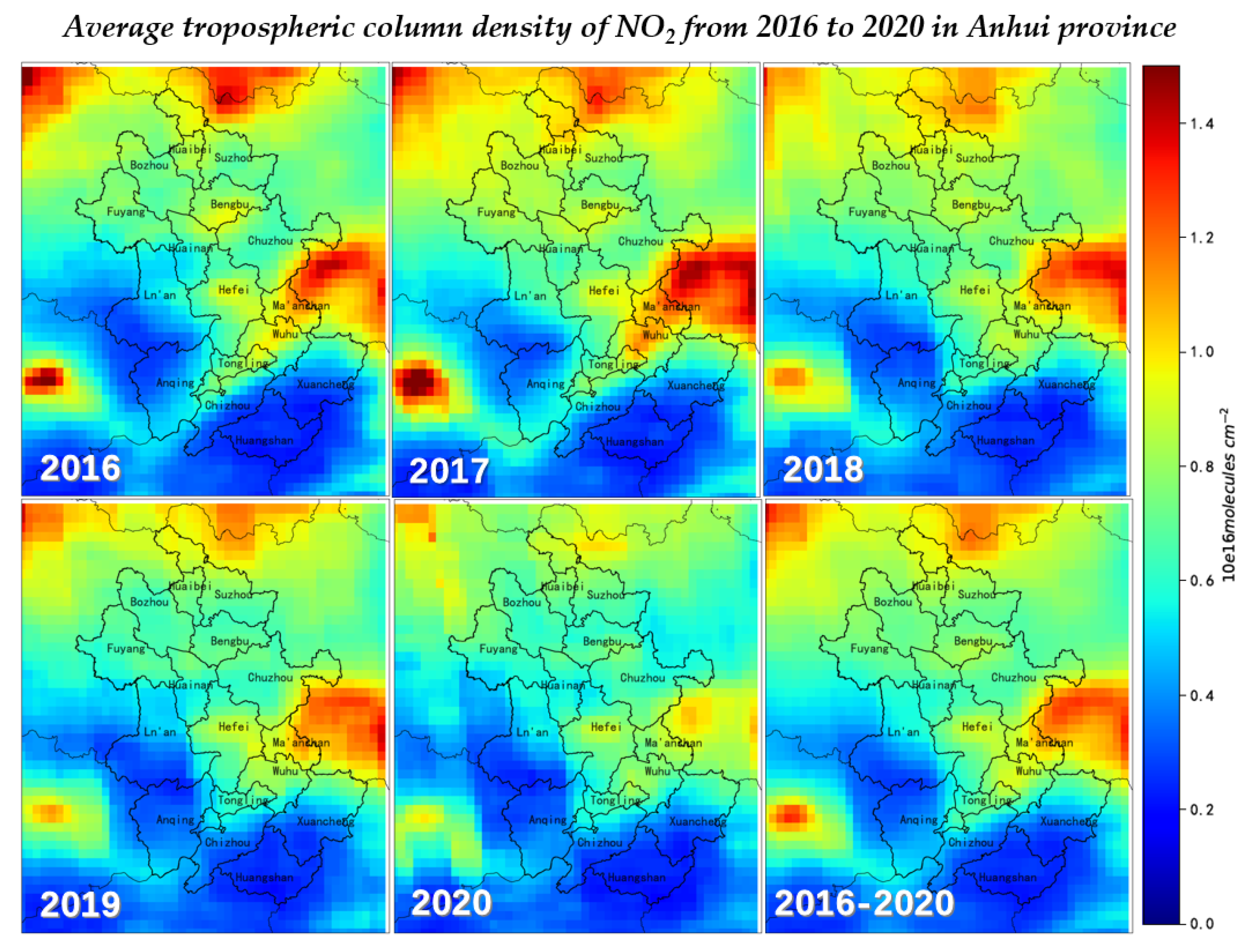
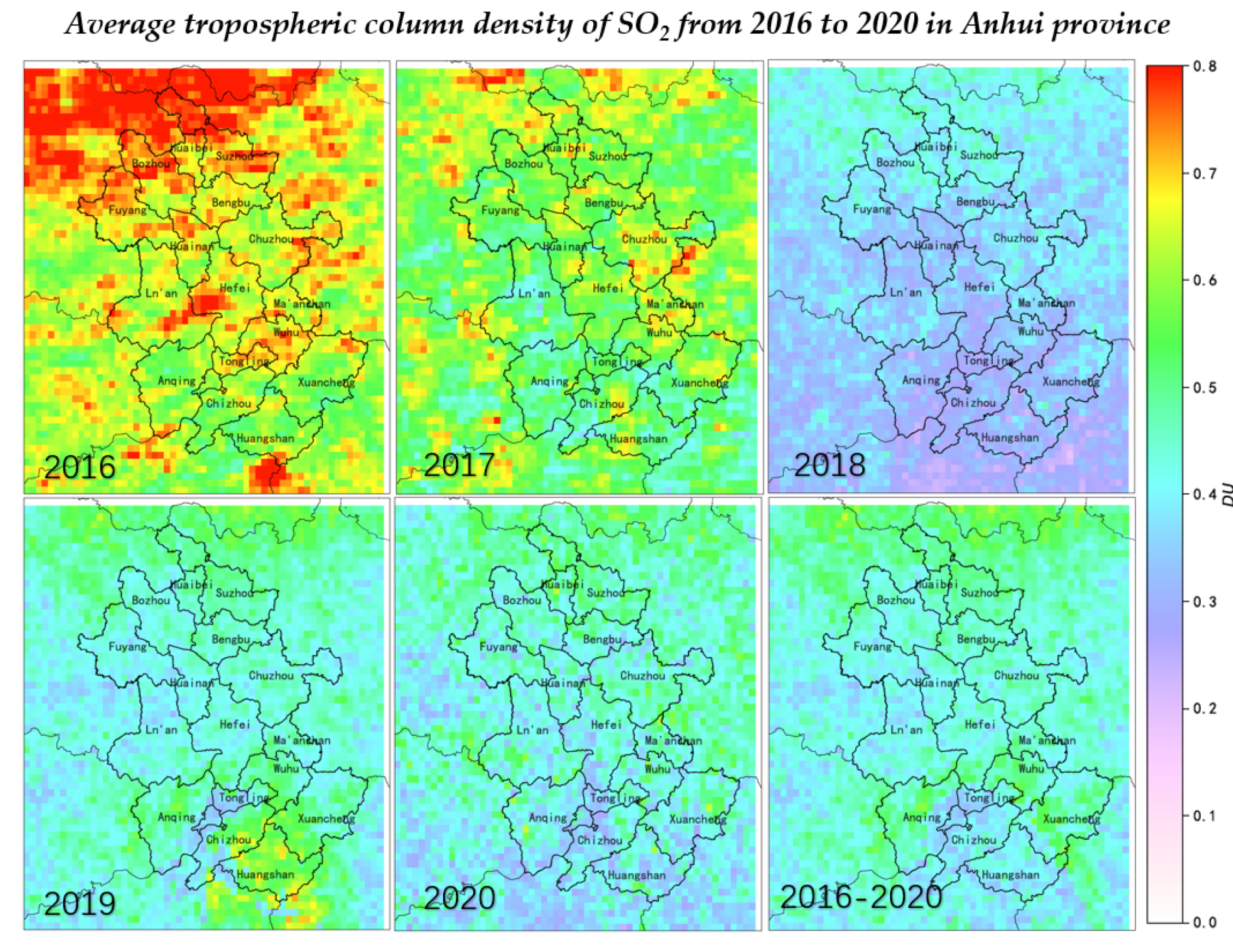
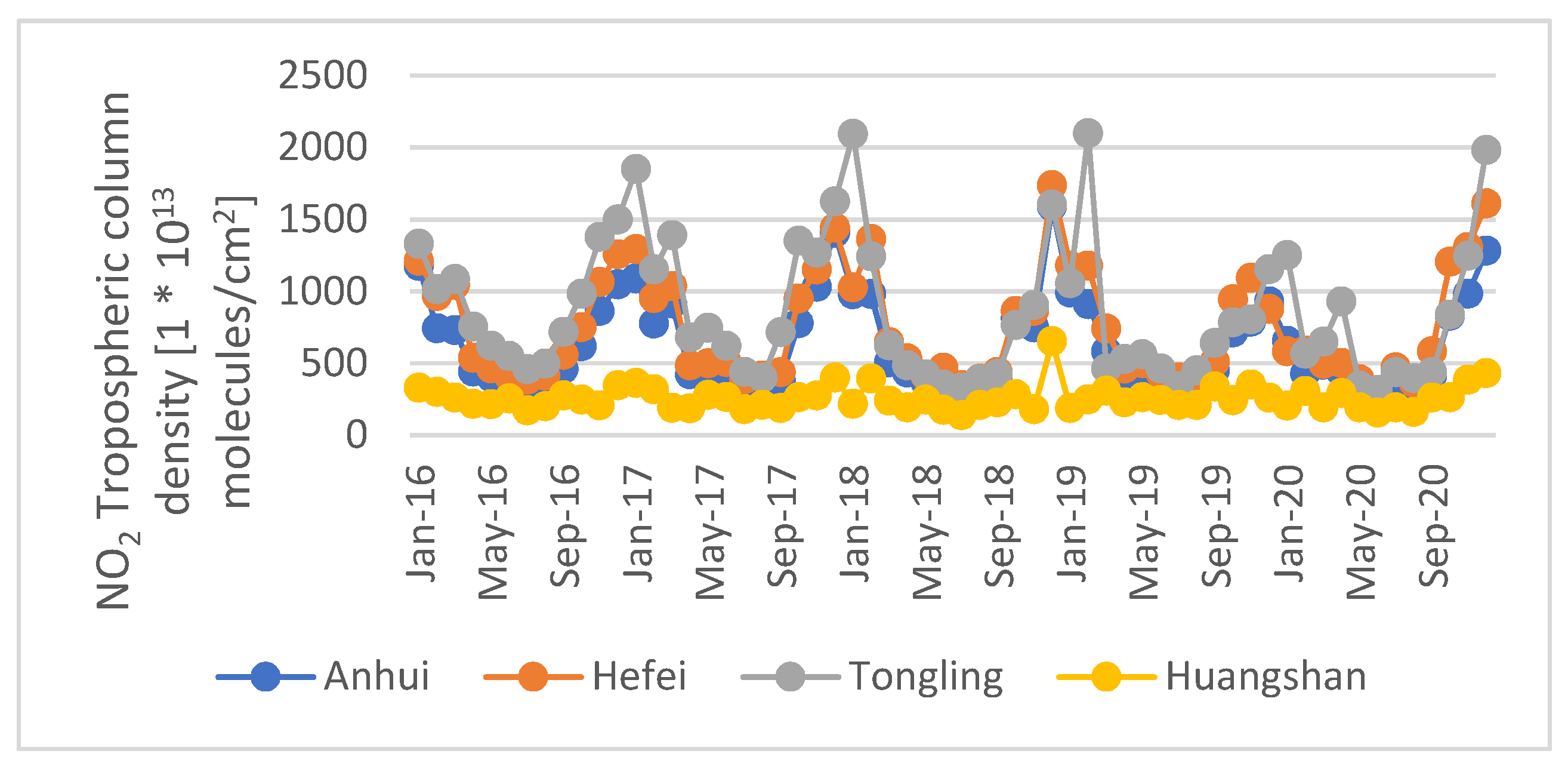
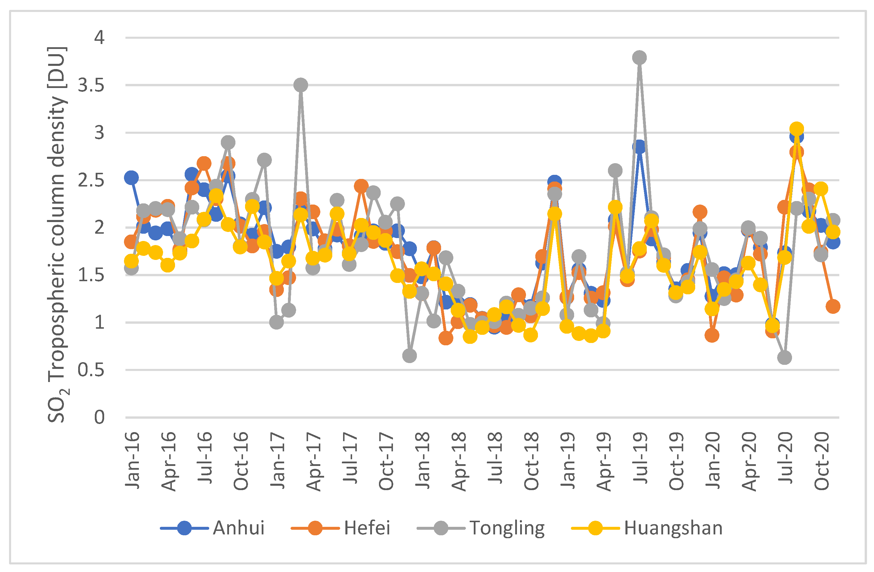
3.1. Temporal Variability of Air Quality in the Anhui Province and Target Cities

3.1.1. Temporal Variability of Atmospheric

Figure 3 shows the monthly mean change of tropospheric NO2 column density in the Anhui province, Hefei, Huangshan and Tongling from 2016 to 2020.
The average NO2 concentration in the Anhui province, Hefei and Tongling was about 1000 × 1013 molecules/cm2, whereas in Huangshan it, was only about 250 × 1013 molecules/cm2. The overall NO2 changes in the Anhui province, Hefei and Tongling showed that the monthly average NO2 had a cyclical characteristic of being “high in winter and low in summer”. NO2 concentrations peaked at about 2000 × 1013 molecules/cm2 around January each year and reached the lowest level at about 700 × 1013 molecules/cm2 around July.
The concentration of NO2 in Hefei was similar to that of Tongling and slightly higher than the Anhui province as a whole. The temporal change was similar, with a cyclical change characteristic of “high in winter and low in summer”. The seasonal variation of NO2 can be dominated by the lifetime variation of NO2 due to the temperature and solar radiation varying with seasons [42]. Moreover, NOx emissions also were reported to be with seasonal variations elsewhere. For example, the coal consumption increases during the heating season in winter over North China [43].
As a major tourist city in the Anhui province, the NO2 level of Huangshan was lower than that of Hefei and Tongling, as well as the Anhui province overall. NO2 in Huangshan did not have temporal variation characteristics and fluctuated throughout the year. Except for the high concentration of 600 × 1013 molecules/cm2 in December 2018, the overall variability was within 130–500 × 1013 molecules/cm2. The maximum NO2 levels in winter for the Anhui province and all three cities increased in 2016, 2017 and 2018, to 1100 × 1013, 1400 × 1013 and 1600 × 1013 molecules/cm2, respectively. However, in late 2019 and early 2020, NO2 significantly decreased due to the influence of the novel coronavirus. In December 2019, the overall NO2 concentration in the Anhui province was only 900 × 1013 molecules/cm2. As the whole province began to resume work and production in March and April 2020, NO2 in Tongling had a second peak value, reaching 900 × 1013 molecules/cm2 in April 2020.
By the end of 2020, the NO2 levels in the Anhui province as a whole and the three cities reached their winter peak values again. Peak levels were similar to those in late 2018 and early 2019. The respective concentrations in December 2020 were 1300 × 1013, 1600 × 1013, 400 × 1013 and 200 × 1013 molecules/cm2.

3.1.2. Temporal Variability of Atmospheric SO2

Figure 4 shows the monthly mean change in tropospheric SO2 column density for the Anhui province, Hefei, Huangshan and Tongling from 2016 to 2020.
SO2 concentrations had no clear periodicity in the Anhui province overall or Hefei and Huangshan. The average concentration in the Anhui province from 2016 to 2017 was about 2 DU (Dobson Unit, 1 DU = 2.6867 × 10²⁰ molecules/m2), and it fluctuated throughout the year. The summer of 2016 brought a higher concentration of about 2.5 DU. A lower concentration of about 1.7 DU occurred in the spring of 2017. Compared with 2016 and 2017, SO2 in the first half of 2018 significantly decreased and was relatively stable at about 1 DU. The concentration peaked at about 2.2 DU in December 2018. In 2019 and 2020, SO2 in the Anhui province, Hefei and Huangshan increased compared to 2018, with an average concentration of about 1.6 DU, and there was more intra-year fluctuation in 2019 and 2020 than before, with a peak level of 3 DU per month in the summer of 2019 and 2020. SO2 levels in Tongling were similar to the other study areas, but the variability was more obvious. It reached a low level of about 0.6 DU in December 2017 and July 2020, and high levels of about 3.5 and 3.8 DU appeared in April 2017 and July 2019, respectively.
In addition, peak SO2 in Tongling in March 2017 and July 2019 was significantly different from Hefei, Tongling and the Anhui province as a whole. SO2 for the Anhui province was similar to Hefei, Tongling and Huangshan with similar change trends. The industrial structure of the three cities did not lead to significant differences in urban SO2 levels.

3.1.3. Temporal Variability of Atmospheric CO

Figure 5 shows the monthly variability of atmospheric CO concentration in Hefei, Tongling and Huangshan from January 2016 to December 2020.
The atmospheric CO in Tongling, Hefei and Huangshan was in a state of decline. The average atmospheric CO concentration for the three cities in 2017 were 1.05, 0.92 and 0.68 mg/m3, respectively. In 2020, average concentrations were 0.82, 0.66 and 0.54 mg/m3, respectively, decreasing by 22%, 28% and 21%. Ranked from high to low, the atmospheric CO levels of the three cities were Tongling, Hefei and Huangshan. From 2016 to 2020, average concentrations were 1.0, 0.8 and 0.6 mg/m3, respectively. As a mineral resource-based city, Tongling discharged more CO into the atmosphere by fuel combustion. As a tourist city, Huangshan maintained a low CO level. The variation of atmospheric CO concentration in the three cities showed the periodic characteristics of high in winter and low in summer. This periodic variability in Hefei and Tongling was more obvious. The average CO concentrations in January, from 2016 to 2020, were 1.08 and 1.22 mg/m3, respectively, whereas in July, they were 0.67 and 0.85 mg/m3, 44% and 30% lower than average levels in January, respectively.

3.2. The Relationship between Economic Indexes and Air Pollution

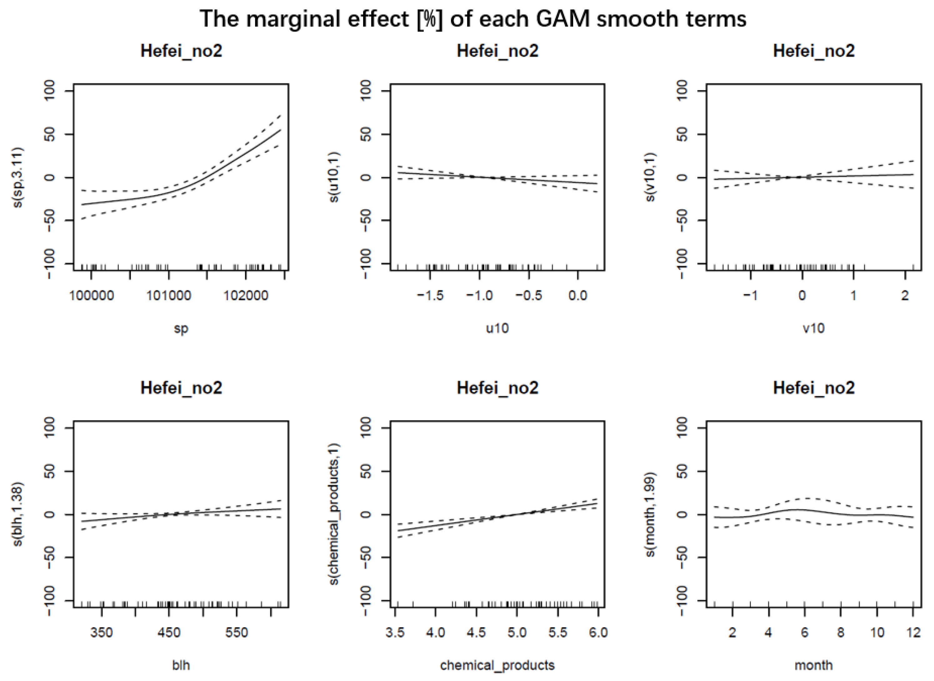
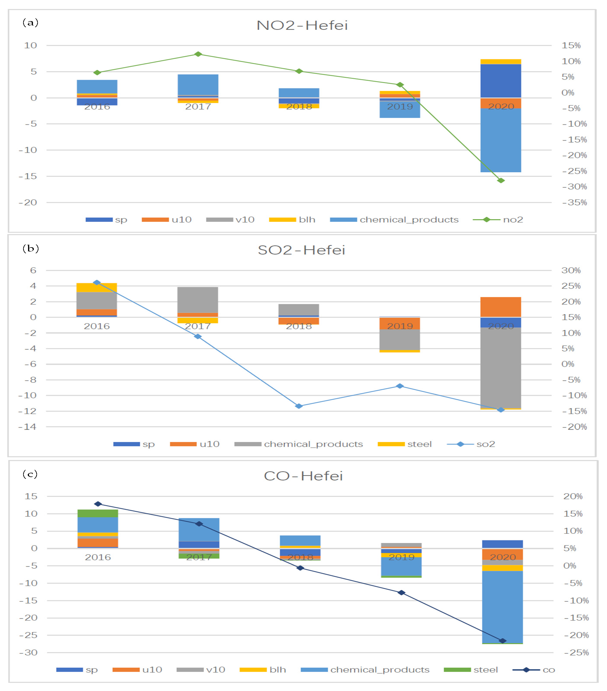
3.2.1. The Relationship between Economic Indexes and Air Pollution in Hefei

Table 1 shows the meanings of meteorological factors and industrial productions.
Figure 6 shows the marginal effect of meteorological factors and industrial product output on atmospheric NO2 column density in Hefei.
The chemical product outputs included agricultural fertilizer production, synthetic detergent production, plastic tire production, plastic products production and chemical fiber production after normalization. Nitrogen fertilizer production can directly or indirectly cause NO2 pollution in the atmosphere. In the process of synthetic detergent production, the hot blast stove, tail gas from the top of the tower and chemical production will generate NO2 pollution. The combustion and chemical processes used in plastic production generate NO2 pollution. In the figure above, increasing chemical product outputs increased the NO2 level, and there was a positive linear correlation between chemical product outputs and atmospheric NO2 content. When the outputs (after normalization) increased by one unit, its effect on atmospheric NO2 content increased by about 20%.
At the beginning of 2020, due to the impact of COVID-19, chemical product output in Hefei decreased significantly to 3.54 units, which was the lowest level from 2016 to 2020. In January and February of 2020, total agricultural chemical fertilizer output was 39,000 tons, with a year-on-year increase of −24.3%. The output of synthetic detergents was 71,400 tons, up 2.9%. Outer rubber tire output was 2.5816 million, up by −37.5%. The output of plastic products was 67,600 tons, up −16.6%, and that of chemical fibers was 10,100 tons, up −16.6%. In March 2018, chemical product output was 5.98 units, the highest level between 2016 and 2020, where the output of agricultural chemical fertilizer was 30,500 tons, an increase of 4.2% year-on-year. The output of synthetic detergents was 37,100 tons, up 8.5%. The rubber tire output was 4.436,600 pieces, up by −2.5%. The output of plastic products was 42,400 tons, up 8.2%. The output of chemical fiber was 9800 tons, up 19.7%. Compared with January and February 2020, the effect of chemical product production on atmospheric NO2 content in March 2018 increased by about 30%.
The marginal effect of meteorological factors and industrial product output on atmospheric SO2 column density in Hefei is shown in Figure S1 in the Supplementary Materials. Rubber tires produce sulfur oxide pollution in the process of vulcanization. The combustion and chemical processes of plastic production generate SO2 pollution. During chemical fiber production, the waste gas in the raw material workshop and the spinning workshop contains SO2 pollution. SO2 pollution is produced during the coking and sintering processes of steel production. As can be seen from the figure, chemical product output increases caused SO2 levels to go up. When chemical product output (after normalization) increased by one unit, the atmospheric SO2 content increased by about 10%. Steel production also had a positive correlation with atmospheric SO2. In May 2020, steel production was the lowest during the research period at 87,700 tons, with a year-on-year increase of -18.8%. In December 2016, steel production was the highest, with a year-on-year increase of 14.5%. The difference in the impact of the two processes on atmospheric SO2 was about 10%.
The marginal effect of meteorological factors and industrial product output on atmospheric CO in Hefei is shown in Figure S2 in the Supplementary Materials. Insufficient combustion of fuel in the production of chemical products led to CO pollution. CO pollution was generated during steel combustion processes, coking and sintering. As can be seen from the figure, chemical product output and steel output increases led to an increase in atmospheric CO. When chemical and steel product output increased by one unit, the atmospheric CO content increased by 25% and 20%, respectively. Compared with January and February 2020, the effect of chemical production in March 2018 on atmospheric CO content increased by about 50%. Compared with May 2020, the effect of steel production in December 2016 on atmospheric CO content increased by about 25%.

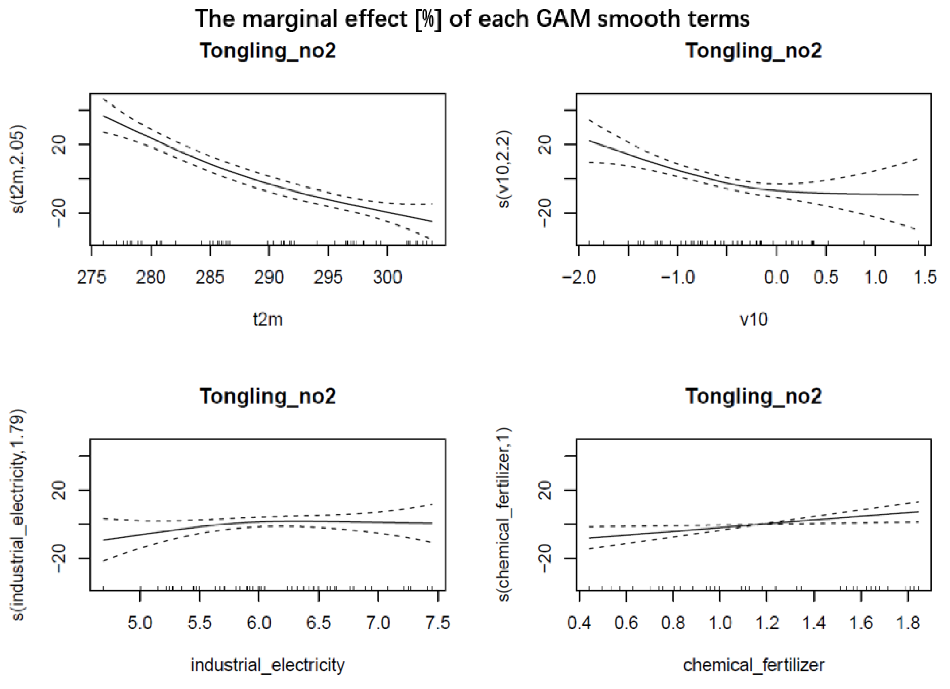
3.2.2. The Relationship between Economic Indexes and Air Pollution in Tongling

The meanings of meteorological factors and industrial productions are shown in Table 2.
Figure 7 shows the marginal effect of meteorological factors and industrial product output on atmospheric NO2 in Tongling. The increase in industrial electricity consumption increased industrial production activities; however, the increase in the demand for electricity generation increased atmospheric NO2 emissions from traffic and combustion emissions to increase the atmospheric NO2 level.
As can be seen in the figure, as industrial electricity consumption increased, the NO2 level also increased. When industrial electricity consumption increased from 469 million to 60 million kWh, atmospheric NO2 content increased by about 10%. When the industrial electricity consumption reached 60 million kWh, the influence on atmospheric NO2 was no longer obvious. An increase in chemical fertilizer yield promoted an increase in NO2 levels. The chemical fertilizer yield in November 2018 was the lowest during the study period (24,000 tons), and the yield in July 2017 was the highest (40,000 tons). The difference in the effect of the two on atmospheric NO2 content was about 15%.
The marginal effect of meteorological factors and industrial product output on atmospheric SO2 concentration in Tongling is shown in Figure S3 in the Supplementary Materials. The production of metal materials was generally accompanied by the combustion process, and the increase in sulfur fuel combustion led to an increase in the atmospheric SO2 level. As can be seen from the figure, increased production of metal materials (electrolytic copper, copper and steel) caused an increase in the SO2 level. In January and February 2019, the cumulative output of electrolytic copper is 88,000 tons, with a year-on-year growth of 26%; the cumulative output of copper was 220,000 tons, with a year-on-year growth of 35%; the cumulative output of steel was 230,000 tons, with a year-on-year growth of 19.2%, corresponding to 2.06 units after normalization. In May 2017, electrolytic copper, copper and steel in Tongling outputs were 106,000, 167,000 and 158,000 tons, respectively, corresponding to 3.44 units after normalization. Compared with the former, the effect of the latter on atmospheric SO2 content increased by about 30%. When the yield reached a certain level (3.5 units after normalization), the influence on SO2 was stable. In April 2020, the electrolytic copper output in Tongling was 80,000 tons, copper was 154,000 tons, steel was 301,000 tons, corresponding to 4.08 units after normalization. Compared with May 2017, the effects of the two on atmospheric SO2 content were nearly the same.
The marginal effect of meteorological factors and industrial product output on atmospheric CO in Tongling is shown in Figure S4 in the Supplementary Materials. When the metal material output changed from 2.06 units (electrolytic copper output 88,000 tons, copper output 220,000 tons and steel output 230,000 tons) in January and February 2019 to 4.08 units (electrolytic copper output 80,000 tons, copper output 154,000 tons, steel output 301,000 tons) in April 2020, there was not a clear impact on atmospheric CO content, and the variability was within 15%.

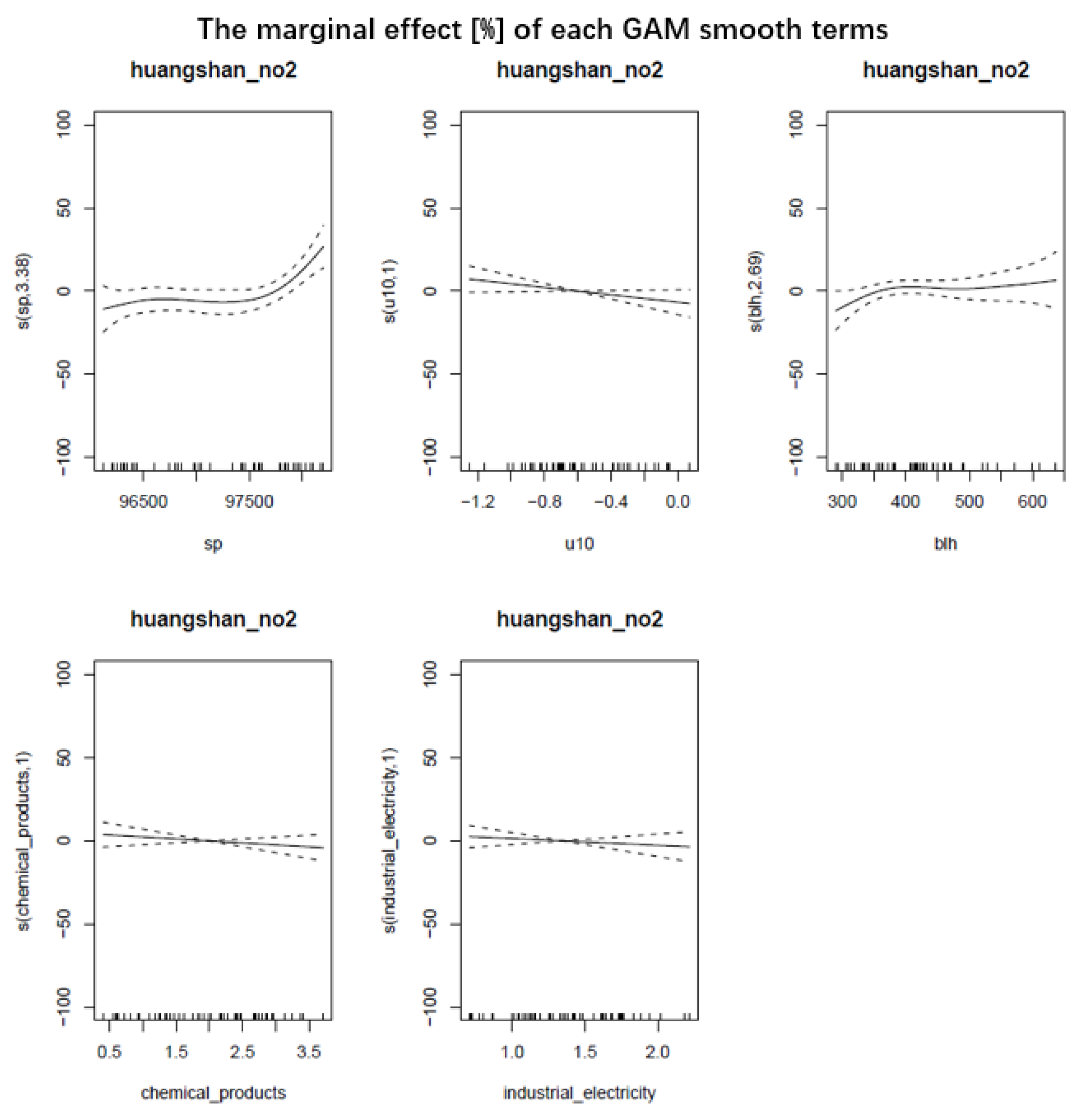
3.2.3. The Relationship between Economic Indexes and Air Pollution in Huangshan

The meanings of meteorological factors and industrial productions are shown in Table 3.
Figure 8 shows the marginal effect of meteorological factors and industrial product output on atmospheric NO2 in Huangshan. The results show that chemical products and industrial electricity have little influence on NO2 change in Huangshan city. The marginal effect of meteorological factors and industrial product output on atmospheric SO2 concentration in Huangshan is shown in Figure S5 in the Supplementary Materials. The results show that cement products have little influence on SO2 change in Huangshan city. The marginal effect of meteorological factors and industrial product output on atmospheric CO is shown in Figure S6 in the Supplementary Materials. The results show that chemical products have little influence on CO change in Huangshan city.
As a major tourist city in the Anhui province, NO2 in Huangshan was significantly lower than in Hefei and Tongling, as well as the Anhui province overall. Moreover, there was no clear temporal variability in NO2 for Huangshan. There was no clear periodicity in SO2 concentrations. The CO concentrations remained basically low. Because Huangshan industrial products made up a small proportion of the overall economic volume, the results on industrial production and air quality were not obvious for reference.

4. Discussion

Natural resource scarcity and the destruction of the environment have pushed humanity to a critical stage where changes must be made. Green economic development has become the only choice for mankind. Research on the relationship between the environment and economic development should not only evaluate the current situation but also have practical significance for green economic development. Research on the relationship between industrial products and air pollutants can provide accurate guidance for adjusting economic structure and environmental protection in target areas from a micro point of view. Air pollutant variability is affected by many factors. In addition to the influence of the emitters themselves, meteorological factors have a decisive influence. In our study, we used the regression method to identify relationships between air composition and meteorological factors in the target area and eliminate the influence of meteorological factors. Atmospheric pollutant data that are closely related to industrial production were collected by remote sensing technology. Meteorological data for the target area was obtained from the public dataset ERA-5 of the European Centre for Medium Range Weather Forecasts (ECWMF). Then we collected output industrial production data from 2016 to 2020 for three representative cities in the Anhui province: Hefei (technology-based industry), Tongling (resource-based industry) and Huangshan (tourism-based industry). A generalized additive model was used to fit the relationship between air pollutants and industrial production.
In Hefei, when chemical product output (after normalization) increases by one unit, its effect on atmospheric NO2 content increases by about 20%. When the chemical product output (after normalization) increased by one unit, the atmospheric SO2 content increased by about 10%. When the output of chemical and steel products increased by one unit, the atmospheric CO content increased by 25% and 20%, respectively.
Figure 9 below is the comparison of inter-annual variations between air pollutants and GAMs smoothing terms over Hefei.
In Tongling, when industrial electricity consumption increased from 469 million to 60 million kWh, atmospheric NO2 content increased by about 10%. When chemical fertilizer yield increased from 24,000 to 40,000 tons, atmospheric NO2 content increased by about 15%. When the output of metal materials increased from 2.06 units to 3.44 units, atmospheric SO2 content increased by about 30%. When the output of metal materials reached 4.08 units, atmospheric SO2 content remained stable. The metal material yield impacts on atmospheric CO content were not obvious, and the total effect was within 15%.
In Huangshan, NO2, SO2 and CO concentrations were far lower than the average level of the whole province, and there were no clear changes. The proportion of industrial products in overall economic volume was small, and the results for industrial production and air quality were not obvious for reference.
The comparison of inter-annual variations between air pollutants and GAMs smoothing terms over Tongling and Huangshan are shown in Figures S7 and S8 in the Supplementary Materials, respectively.
Future work can be continued on typical cities with different compositions of industrial production. With the support of sufficient cases and data, the optimal industrial product proportion structure is analyzed according to the meteorological conditions of different regions.

5. Conclusions

Our methods produced different results for different cities because of differences in air quality, meteorology and economic structure. However, this research method can be applied to different objectives with sufficient data support. The results of this study can help relevant units and departments predict local economic development trends according to air quality change. They can also help departments adjust local industrial structure according to the requirements of environmental protection policies, optimize economic development plans and enhance the ability of environmental protection and supervision. This study has important practical significance, not only for the transformation and upgrading of cities in China but other appropriate research targets on a global scale.

Supplementary Materials

The following are available online at https://0-www-mdpi-com.brum.beds.ac.uk/article/10.3390/rs13163137/s1, Figure S1. The marginal effect [%] of each GAM smooth term on SO2 pollution over Hefei; Figure S2. The marginal effect [%] of each GAM smooth term on CO pollution over Hefei; Figure S3. The marginal effect [%] of each GAM smooth term on SO2 pollution over Tongling; Figure S4. The marginal effect [%] of each GAM smooth term on CO pollution over Tongling; Figure S5. The marginal effect [%] of each GAM smooth term on SO2 pollution over Huangshan; Figure S6. The marginal effect [%] of each GAM smooth term on CO pollution over Huangshan; Figure S7. The inter-annual variations of air pollutants concentration and the corresponding GAMs smooth terms accounted by each variable; Figure S8. The inter-annual variations of air pollutants concentration and the corresponding GAMs smooth terms accounted by each variable; Table S1 is the input data of Hefei city; Table S2 is the input data of Tongling city; Table S3 is the input data of Huangshan city.

Author Contributions

Conceptualization, C.T. and C.L.; methodology, C.Z.; software, C.Z.; validation, C.Z.; formal analysis, C.T.; investigation, C.T.; resources, C.T.; data curation, C.T.; writing—original draft preparation, C.T.; writing—review and editing, C.T.; visualization, C.T.; supervision, C.T.; project administration, C.T. All authors have read and agreed to the published version of the manuscript.

Funding

This research was supported by the China Postdoctoral Science Foundation (2020TQ0320 and 2021M693068), and the Fundamental Research Funds for the Central Universities.

Institutional Review Board Statement

Not applicable.

Informed Consent Statement

Not applicable.

Data Availability Statement

The data that support the findings of this study are available from the author upon reasonable request.

Acknowledgments

We thank NASA for sharing the data acquired from the Ozone Monitoring Instrument (OMI) on-board the EOS-Aura satellite. We thank the Chinese National Environment Monitoring Center (CNEMC) for the data support from in situ measurements. We thank the support from the Anhui Provincial Bureau of Statistics. We thank the European Centre for Medium Range Weather Forecasts (ECWMF) for the meteorological parameters from the ERA-5 products. We express our heartfelt thanks to Academician Shanlin Yang and Professor Shuai Ding from Hefei University of Technology for the guidance and inspiration.

Conflicts of Interest

The authors declare no conflict of interest.

References

  1. UNEP. Towards a Green Economy: Pathways to Sustainable Development and Poverty Eradication. Nairobi Kenya Unep. 2011. Available online: http://citeseerx.ist.psu.edu/viewdoc/download?doi=10.1.1.642.2587&rep=rep1&type=pdf (accessed on 20 April 2021).
  2. Li, J.; Lin, B. Green Economy Performance and Green Productivity Growth in China’s Cities: Measures and Policy Implication. Sustainability 2016, 8, 947. [Google Scholar] [CrossRef] [Green Version]
  3. Zan, Z. Relation between Chinese Industrialization Level and Environmental Quality. 2006. Available online: http://en.cnki.com.cn/Article_en/CJFDTOTAL-CJKX200602009.htm (accessed on 20 April 2021).
  4. Chen, S.S.; Zhang, X.Q.; University, H. Research on the Industrial Transformation and Upgrading in China and the Competitive Advantages of Rapid Growth in Economy under the Connectivity Blueprint. 2019. Available online: http://en.cnki.com.cn/Article_en/CJFDTotal-KXGY201903014.htm (accessed on 15 March 2021).
  5. Government Work Report [R]. 2021. Available online: http://www.gov.cn/guowuyuan/zfgzbg.htm (accessed on 15 March 2021).
  6. Foray, D.; Gruebler, A. Technology and the environment: An overview. Technol. Forecast. Soc. Chang. 1996, 53, 3–13. [Google Scholar] [CrossRef] [Green Version]
  7. Murphy, J.; Gouldson, A. Environmental policy and industrial innovation: Integrating environment and economy through ecological modernisation. Geoforum 2010, 31, 33–44. [Google Scholar] [CrossRef]
  8. Grossman, G.M.; Krueger, A.B. Environmental Impacts of a North American Free Trade Agreement. CEPR Discuss. Pap. 1992, 8, 223–250. [Google Scholar]
  9. Xu, Q.; Dong, Y.X.; Yang, R. Urbanization impact on carbon emissions in the Pearl River Delta region: Kuznets curve relationships. J. Clean. Prod. 2018, 180, 514–523. [Google Scholar] [CrossRef]
  10. Stern, D.I. The Rise and Fall of the Environmental Kuznets Curve. World Dev. 2004, 32, 1419–1439. [Google Scholar] [CrossRef]
  11. Cole, M.A. Development, trade, and the environment: How robust is the Environmental Kuznets Curve? Environ. Dev. Econ. 2003, 8, 557–580. [Google Scholar] [CrossRef]
  12. Chapman, S.D. Economic growth, trade and energy: Implications for the environmental Kuznets curve. Ecol. Econ. 1998, 25, 195–208. [Google Scholar]
  13. Du, G.; Liu, S.; Lei, N.; Yong, H. A test of environmental Kuznets curve for haze pollution in China: Evidence from the penal data of 27 capital cities. J. Clean. Prod. 2018, 205, 821–827. [Google Scholar] [CrossRef]
  14. Dong, C.; Ramirez, C.D. Air Pollution, Government Pollution Regulation, and Industrial Production in China. J. Syst. Sci. Complex. 2020, 33, 1064–1079. [Google Scholar]
  15. Smeets, E.; Weterings, R. Environmental Indicators: Typology and Overview. 1999. Available online: http://www.geogr.uni-jena.de/fileadmin/Geoinformatik/projekte/brahmatwinn/Workshops/FEEM/Indicators/EEA_tech_rep_25_Env_Ind.pdf (accessed on 24 February 2021).
  16. Liu, J.H.; Chen, Y.F.; Lin, T.S.; Chen, C.P.; Chen, P.T.; Wen, T.H.; Sun, C.H.; Juang, J.Y.; Jiang, J.A. An Air Quality Monitoring System for Urban Areas Based on the Technology of Wireless Sensor Networks. Int. J. Smart Sens. Intell. Syst. 2012, 5, 191–214. [Google Scholar] [CrossRef] [Green Version]
  17. Zhang, C.; Liu, C.; Hu, Q.; Cai, Z.; Liu, J. Satellite UV-Vis spectroscopy: Implications for air quality trends and their driving forces in China during 2005–2017. Light Sci. Appl. 2019, 8, 100. [Google Scholar] [CrossRef] [PubMed] [Green Version]
  18. Levelt, P.F.; Oord, G.; Dobber, M.R.; Mlkki, A.; Saari, H. The Ozone Monitoring Instrument. IEEE Trans. Geosci. Remote Sens. 2006, 44, 1093–1101. [Google Scholar] [CrossRef]
  19. Levelt, P.F.; Joiner, J.; Tamminen, J.; Veefkind, J.P.; Bhartia, P.K.; Stein Zweers, D.C.; Duncan, B.N.; Streets, D.G.; Eskes, H.; McLinden, C.; et al. The Ozone Monitoring Instrument: Overview of 14 years in space. Atmos. Chem. Phys. 2018, 18, 5699–5745. [Google Scholar] [CrossRef] [Green Version]
  20. Tian, Z.; Wza, B.; Ry, C.; Yla, B.; Mja, B. CO2 capture and storage monitoring based on remote sensing techniques: A review. 2020. Available online: https://0-www-sciencedirect-com.brum.beds.ac.uk/science/article/abs/pii/S0959652620344541 (accessed on 13 April 2021).
  21. Wu, X.; Wang, L.; Zheng, H. A network effect on the decoupling of industrial waste gas emissions and industrial added value: A case study of China. J. Clean. Prod. 2019, 234, 1338–1350. [Google Scholar] [CrossRef]
  22. Dang, H.; Trinh, T.A. Does the COVID-19 lockdown improve global air quality? New cross-national evidence on its unintended consequences. J. Environ. Econ. Manag. 2021, 105, 102401. [Google Scholar] [CrossRef]
  23. Brodeur, A.; Cook, N.; Wright, T. On the effects of COVID-19 safer-at-home policies on social distancing, car crashes and pollution. J. Environ. Econ. Manag. 2021, 106, 102427. [Google Scholar] [CrossRef]
  24. Hu, F.; Guo, Y. Impacts of electricity generation on air pollution: Evidence from data on air quality index and six criteria pollutants. SN Appl. Sci. 2021, 3, 1–10. [Google Scholar] [CrossRef]
  25. Xu, W.; Sun, J.; Liu, Y.; Xiao, Y.; Tian, Y.; Zhao, B.; Zhang, X. Spatiotemporal variation and socioeconomic drivers of air pollution in China during 2005-2016. J. Environ. Manag. 2019, 245, 66–75. [Google Scholar] [CrossRef] [PubMed]
  26. Xie, Y.; Wu, D.; Zhu, S. Can new energy vehicles subsidy curb the urban air pollution? Empirical evidence from pilot cities in China. Sci. Total Environ. 2021, 754, 142232. [Google Scholar] [CrossRef]
  27. Wx, A.; Jing, Z.A.; Chao, Z.B.; Xl, B.; Jing, W. Spatiotemporal PM 2.5 variations and its response to the industrial structure from 2000 to 2018 in the Beijing-Tianjin-Hebei region. J. Clean. Prod. 2020, 279, 123742. [Google Scholar]
  28. Yang, Z.; Yang, J.; Li, M.; Chen, J.; Ou, C.Q. Nonlinear and lagged meteorological effects on daily levels of ambient PM2.5 and O3: Evidence from 284 Chinese cities. J. Clean. Prod. 2020, 278, 123931. [Google Scholar] [CrossRef]
  29. Su, T.; Li, Z.; Kahn, R. Relationships between the planetary boundary layer height and surface pollutants derived from lidar observations over China: Regional pattern and influencing factors. Atmos. Chem. Phys. 2018, 18, 15921–15935. [Google Scholar] [CrossRef] [Green Version]
  30. Su, T.; Li, Z.; Zheng, Y.; Luan, Q.; Guo, J. Abnormally shallow boundary layer associated with severe air pollution during the COVID-19 lockdown in China. Geophys. Res. Lett. 2020, 47, e2020GL090041. [Google Scholar] [CrossRef] [PubMed]
  31. Xz, A.; Zhen, W.; Mc, C.; Xw, A.; Nan, Z.A.; Jx, D. Long-term ambient SO2 concentration and its exposure risk across China inferred from OMI observations from 2005 to 2018. Atmos. Res. 2020, 247, 105150. [Google Scholar]
  32. Xue, R.; Wang, S.; Li, D.; Zou, Z.; Zhou, B. Spatio-temporal variations in NO2 and SO2 over Shanghai and Chongming Eco-Island measured by Ozone Monitoring Instrument (OMI) during 2008–2017. J. Clean. Prod. 2020, 258, 120563. [Google Scholar] [CrossRef]
  33. Zhang, C.; Liu, C.; Chan, K.L.; Hu, Q.; Liu, J. First observation of tropospheric nitrogen dioxide from the Environmental Trace Gases Monitoring Instrument onboard the GaoFen-5 satellite. Light Sci. Appl. 2020, 9, 1–9. [Google Scholar] [CrossRef] [Green Version]
  34. Song, Y.Z.; Yang, H.L.; Peng, J.H.; Song, Y.R.; Qian, S.; Li, Y. Estimating PM2.5 Concentrations in Xi’an City Using a Generalized Additive Model with Multi-Source Monitoring Data. PLoS ONE 2015, 10, e142149. [Google Scholar] [CrossRef] [PubMed] [Green Version]
  35. Wu, Z.; Zhang, S. Study on the spatial–temporal change characteristics and influence factors of fog and haze pollution based on GAM. Neural Comput. Appl. 2019, 31, 1619–1631. [Google Scholar] [CrossRef] [Green Version]
  36. Tan, W.; Liu, C.; Wang, S.; Xing, C.; Su, W.; Zhang, C.; Xia, C.; Liu, H.; Cai, Z.; Liu, J. Tropospheric NO2, SO2, and HCHO over the East China Sea, using ship-based MAX-DOAS observations and comparison with OMI and OMPS satellites data. Atmos. Chem. Phys. 2018, 18, 15387–15402. [Google Scholar] [CrossRef] [Green Version]
  37. Monks, P.S.; Granier, C.; Fuzzi, S.; Stohl, A.; Von, G.R. Atmospheric composition change—Global and regional air quality. Atmos. Environ. 2009, 43, 5268–5350. [Google Scholar] [CrossRef] [Green Version]
  38. Huang, Q.; Wang, T.; Chen, P.; Huang, X.; Zhu, J.; Zhuang, B. Impacts of emission reduction and meteorological conditions on air quality improvement during the 2014 Youth Olympic Games in Nanjing, China. Atmos. Chem. Phys. 2017, 17, 1–19. [Google Scholar] [CrossRef] [Green Version]
  39. Foy, B.D.; Lu, Z.; Streets, D.G. Satellite NO2 retrievals suggest China has exceeded its NOx reduction goals from the twelfth Five-Year Plan. Sci. Rep. 2016, 6, 35912. [Google Scholar] [CrossRef] [PubMed] [Green Version]
  40. Wood, S.N. Generalized Additive Models: An Introduction with R, 2nd ed. 2017. Available online: https://0-www-tandfonline-com.brum.beds.ac.uk/doi/abs/10.1198/tech.2007.s505?journalCode=utch20 (accessed on 12 June 2021).
  41. Pearce, J.L.; Beringer, J.; Nicholls, N.; Hyndman, R.J.; Tapper, N.J. Quantifying the influence of local meteorology on air quality using generalized additive models. Atmos. Environ. 2011, 45, 1328–1336. [Google Scholar] [CrossRef]
  42. Schreier, S.F.; Richter, A.; Peters, E.; Ostendorf, M.; Burrows, J.P. Dual ground-based MAX-DOAS observations in Vienna, Austria: Evaluation of horizontal and temporal NO2, HCHO, and CHOCHO distributions and comparison with independent data sets. Atmos. Environ. X 2019, 5, 100059. [Google Scholar] [CrossRef]
  43. Zhao, B.; Zheng, H.; Wang, S.; Smith, K.R.; Lu, X.; Aunan, K.; Gu, Y.; Wang, Y.; Ding, D.; Xing, J. Change in household fuels dominates the decrease in PM2.5 exposure and premature mortality in China in 2005–2015. Proc. Natl. Acad. Sci. USA 2018, 115, 12401–12406. [Google Scholar] [CrossRef] [PubMed] [Green Version]
Figure 1. Average column density of NO2 from 2016 to 2020 in the Anhui province.
Remotesensing 13 03137 g001
Figure 2. Average column density of SO2 from 2016 to 2020 in the Anhui province.
Remotesensing 13 03137 g002
Figure 3. Monthly mean changes of tropospheric NO2 column density.
Remotesensing 13 03137 g003
Figure 4. Monthly mean changes of tropospheric SO2 column density.
Remotesensing 13 03137 g004
Figure 5. Monthly mean changes of CO concentration.
Remotesensing 13 03137 g005
Figure 6. The marginal effect (%) of each GAM smooth term on NO2 pollution over Hefei. The response curve of individual variables, such as sp, u10, v10, blh, chemical_products and month, were shown in different panels.
Remotesensing 13 03137 g006
Figure 7. The marginal effect (%) of each GAM smooth term on NO2 pollution over Tongling.
Remotesensing 13 03137 g007
Figure 8. The marginal effect (%) of each GAM smooth term on NO2 pollution over Huangshan.
Remotesensing 13 03137 g008
Figure 9. The inter-annual variations of air pollutants concentration and the corresponding GAMs smooth terms accounted by each variable. The left y-axis is for the annual mean of smooth terms, and the right y-axis is for the relative change (%) to the overall mean. The results were presented for (a) NO2, (b) SO2 and (c) CO, respectively.
Remotesensing 13 03137 g009
Table 1. The input variables selected for GAMs modeling on the air quality of Hefei city.
NameMeaning
SpSurface pressure
U1010 metre U wind components
V1010 metre V wind components
BlhBoundary layer height
Chemical productsIncluding: agricultural chemical fertilizers, synthetic detergents, rubber tires, plastic products and chemical fibers
SteelSteel production
MonthTime measured in months
Table 2. The input variables selected for GAMs modeling on air quality of Tongling city.
NameMeaning
SpSurface pressure
T2m2 meter temperature
V1010 meter V wind components
BlhBoundary layer height
MonthSeasonal manifestation
Industrial electricityIndustrial electricity consumption
Chemical fertilizerChemical fertilizer yield
MetalIncludes electrolytic copper, copper, steel
Table 3. The input variables selected for GAMs modeling on air quality of Huangshan city.
NameMeaning
SpSurface pressure
U1010 meter U wind components
BlhBoundary layer height
Industrial electricityIndustrial electricity consumption
Chemical productsIncluding: agricultural chemical fertilizers, synthetic detergents, rubber tires, plastic products and chemical fibers
CementBuilding materials
Publisher’s Note: MDPI stays neutral with regard to jurisdictional claims in published maps and institutional affiliations.

