Article

Estimation of Soil Organic Carbon Contents in Croplands of Bavaria from SCMaP Soil Reflectance Composites

1
German Aerospace Center (DLR), German Remote Sensing Data Center (DFD), Muenchener Str. 20, 82234 Wessling, Germany
2
German Aerospace Center (DLR), Remote Sensing Technology Institute (IMF), Muenchener Str. 20, 82234 Wessling, Germany
3
Bavarian State Research Center for Agriculture, Institute for Organic Farming, Soil and Resource Management, Lange Point 6, 85354 Freising, Germany
4
Mitteldeutsches Institut für Angewandte Standortkunde und Bodenschutz (MISB), 06114 Halle, Germany
5
Georges Lemaître Centre for Earth and Climate Research, Earth and Life Institute, Université Catholique de Louvain, 1348 Louvain-la-Neuve, Belgium
*
Author to whom correspondence should be addressed.
Remote Sens. 2021, 13(16), 3141; https://0-doi-org.brum.beds.ac.uk/10.3390/rs13163141
Submission received: 25 June 2021 / Revised: 30 July 2021 / Accepted: 5 August 2021 / Published: 8 August 2021
(This article belongs to the Special Issue Remote Sensing for Soil Organic Carbon Mapping and Monitoring)

Abstract

:
For food security issues or global climate change, there is a growing need for large-scale knowledge of soil organic carbon (SOC) contents in agricultural soils. To capture and quantify SOC contents at a field scale, Earth Observation (EO) can be a valuable data source for area-wide mapping. The extraction of exposed soils from EO data is challenging due to temporal or permanent vegetation cover, the influence of soil moisture or the condition of the soil surface. Compositing techniques of multitemporal satellite images provide an alternative to retrieve exposed soils and to produce a data source. The repeatable soil composites, containing averaged exposed soil areas over several years, are relatively independent from seasonal soil moisture and surface conditions and provide a new EO-based data source that can be used to estimate SOC contents over large geographical areas with a high spatial resolution. Here, we applied the Soil Composite Mapping Processor (SCMaP) to the Landsat archive between 1984 and 2014 of images covering Bavaria, Germany. Compared to existing SOC modeling approaches based on single scenes, the 30-year SCMaP soil reflectance composite (SRC) with a spatial resolution of 30 m is used. The SRC spectral information is correlated with point soil data using different machine learning algorithms to estimate the SOC contents in cropland topsoils of Bavaria. We developed a pre-processing technique to address the issue of combining point information with EO pixels for the purpose of modeling. We applied different modeling methods often used in EO soil studies to choose the best SOC prediction model. Based on the model accuracies and performances, the Random Forest (RF) showed the best capabilities to predict the SOC contents in Bavaria (R² = 0.67, RMSE = 1.24%, RPD = 1.77, CCC = 0.78). We further validated the model results with an independent dataset. The comparison between the measured and predicted SOC contents showed a mean difference of 0.11% SOC using the best RF model. The SCMaP SRC is a promising approach to predict the spatial SOC distribution over large geographical extents with a high spatial resolution (30 m).

1. Introduction

Precise knowledge about the distribution of soil organic carbon (SOC) contents in agricultural soils is a valuable information for, e.g., food security issues [1] or global climate change [2]. The organic carbon stocks in soils represent one of the largest reservoirs in the global carbon cycle [3,4] and are affected by various drivers [5]. Soils with sufficiently high [6,7] and balanced SOC contents are considered healthy soils [8,9] and are less prone to impacts of climate change [7]. Adequate land management is necessary to preserve soil health and soil quality [10] and enables an increase of agroecosystem resiliency [11].
To capture and quantify SOC contents in agricultural soils for efficient and sustainable land use, data with high spatial resolution is needed in order to understand the impacts of climate change on soil quality [12]. High-resolution surveys at the national to regional scale are urgently required, as detailed spatial patterns in SOC are an important aspect for land management at the farm or even the field scale [13]. For applications with a large geographical extent [14] (national to European-wide), SOC maps are mostly available with a spatial resolution of 250 m to 1 km. The European Soil Data Center (ESDAC) provides several pan-European SOC maps. However, both well-known maps OCTOP: Topsoil Organic Carbon Contents for Europe [15] and the Topsoil Soil Organic Carbon Map based on the LUCAS (Land Use/Cover Area frame statistical Survey) soil datasets for EU25 [16] are distributed in a coarse 1 km raster format. The maps have, therefore, a limited suitability as a basis for high-resolution analysis at the farm or even the field scale.
Earth Observation (EO) can be a valuable data-source for area-wide mapping with a resolution that allows distinguishing between or even with field patterns [17]. In this context, hyperspectral (e.g., [18,19,20,21]) and multispectral images (e.g., [22,23,24]) are commonly used EO datasets to derive SOC contents. In Table 1, studies for different European regions are compared regarding their capabilities of SOC modeling. Generally, point soil information was correlated with multi- or hyperspectral pixel values using different machine learning (ML) techniques to derive SOC contents. However, in most studies, the estimation of SOC was restricted to relatively small areas (0.09 to 10.000 km²) in which the soil conditions (bare, smooth and dry soils) were considered to be optimal. This optimization prevented applying the models to cover larger geographical areas, except for a couple of previous efforts [25,26]. Additionally, the use of hyperspectral and multispectral remote sensing data for the estimation of SOC contents and other soil variables is hampered by the need for data that provide bare soil conditions. Mapping of exposed soils and the estimation of soil parameters is challenging due to temporal or permanent vegetation cover [27]. The area of exposed soils on a single remote sensing scene is limited, and often, the periods in which exposed soils dominate are restricted to short time windows [28] when the soil is in seedbed condition. Compositing techniques of multi-temporal satellite image archives provide an alternative and are widely used in the literature [25,26,27,28,29,30,31,32,33,34]. The compositing approach allows combining all bare soils of all input scenes, which enables a joint estimation of soil parameters for all exposed soils in the observed time period. For several years, new compositing techniques were developed in the course of opening the Landsat archive [35] that can retrieve exposed soils from multi-temporal satellite image archives [26,28,36,37]. An averaging of exposed soil areas over several years allows producing a new and spatially enhanced data source for soil analyses. Here, the soil spectra are relatively independent from seasonal differences in soil moisture and other soil surface conditions occurring during rain events or longer drought periods. In the resulting new data source, only permanent spatial soil moisture differences such as for the different soil types and texture characteristics remain. However, an in-depth proof of this assumption has not yet been provided.
The operational Soil Composite Mapping Processor (SCMaP) is a multitemporal compositing approach [36], which enables an automated generation of area-wide soil reflectance composites (SRC) for the estimation of soil parameters using all available multispectral reflectance images for a defined period. So far, SCMaP SRC has not been used as an EO database for the SOC modeling of exposed topsoils in croplands of large geographical extents. Therefore, in this study, the SOC modeling capabilities of the SCMaP SRC are investigated and performed for a large portion of the German federal state of Bavaria and adjacent areas (about 130,000 km²) as solid calibration and validation datasets are available.
Generally, linking point data with EO images (30 m, 20 m pixel resolution) can be considered as a potential source of inaccuracies for soil parameter modeling as not all samples are collected at least 30 m from the field border the sample is related to [38]. In this case, the EO pixel may reflect the signal from adjacent fields with different spectral information, which is related to a single soil sample. New approaches are necessary that can handle the misalignment of the soil database and the spectral pixel information from the EO images for SOC modeling.
Table 1. Overview on soil organic carbon (SOC) modeling studies across different regions in Europe.
Study Area (Size (km²))Earth Observation Data/Soil Data: Number of Samples (Samples/km²)SOC Range (%)Machine Learning AlgorithmRMSE (%)RPDReference
Albany Ticket, South Africa (320)HyMap (hy, A)/125 (0.39) spectra0.21–5.85Feature based MLR (1)0.620.431.57[39]
Loam belt, Belgium (BE) (462)/Luxembourg (LUX) (146)APEX (hy, A)/84 (1.58) (LUX), 54 (0.12) (BE) spectra/LUCAS spectra1.69–31.8PLSR (1)-field spec: 0.49 (LUX)/0.15 (BE)
LUCAS: 0.49 (LUX)/0.15 (BE)
field spec: 1.7 (LUX)/1.4 (BE)
LUCAS: 1.7 (LUX)/1.4 (BE)
[40]
Demmin, Germany (GER) (200)/Loam Belt, BE (426) BE/Gutland-Oesling, LUX (204)Sentinel-2 (S-2) (ms, A) APEX (hy, A), S-2 resampled (ms, A)/170 (0.8) (BE)/194 (0.4) (LUX)/231 (0.12) (GER) samples0.6–1.6PLSR/RF (1)-PLSR: 0.10–0.17 (S-2)/0.11–0.17 (hy)/0.08–0.14 (S-2 res)
RF: 0.2–1.86 (S-2)/0.2–1.84 (hy)/0.2–1.86 (S-2 res)
PLSR: 1.0–1.7 (S-2)/1.1–1.7 (hy)/1.0–1.5 (S-2 res)
RF: 1.0–1.5 (S-2)/1.0–2.1 (hy)/1.0–2.1 (S-2 res)
[22]
Demmin, GER (10.000)S-2B (ms, A)/35 LUCAS spectra0.5–38.4RF (1)-0.68–2.670.9–4.4[41]
Demmin, GERS-2 (ms, A), HySpex (hy, A), EnMAP simulated (hy, A)/181 samples0.6–19.4RF (1)-8.7–17.8 (S-2)/11.0–18.8 (EnMAP)1.2–2.5 (S-2)/1.2–2.0 (EnMAP)[42]
Wallonia, BE (3.630)Sentinel-2 (ms, B)/137 (0.038) samples0.67–2.1PLSR (2)0.14 ± 0.03–0.54 ± 0.120.209 ± 0.039–0.363 ± 0.036 1.06 ± 0.06–1.68 ± 0.45[43]
4 fields, Czech Republic (CZK) (0.7–7.76)CASI (hy, A), Sentinel-2 (ms, A)/200 samples)0.56–2.62support vector machine regression (1)-0.12–7.95 (hy)/0.14–9.15 (S-2)1.03–2.05 (hy)/0.89–1.92 (S-2)[44]
4 fields, Lower Rhine Basin (GER) (0.0025–0.09) HyMap (hy, A)/204 samples0.8–1.85PLSR (2)0.34–8.830.76–1.131.14–2.32[45]
EuropeLandsat-4, -5, -7, -8 composite (1982–2018) (ms, B)/LUCAS spectra0.0–43.84gradient boosting trees (1)0.06–0.131.52–1.680.52–0.58[25]
Wulfen, GER (200) GERHyMap (hy, A)/73 (0.73) samples0.7–3.85MLR/PLSR (2)0 90 (PLSR)/0.86 (MLR)0.29 (PLSR)/0.22 (MLR)-[46]
Versailles Plains (VP), (221)/Peyne Valley (PV), France (FRA) (48)S-2 (ms, A)/72 (0.33) (VP), 143 (2.98) (PV) samples0.7–3.19 (VP)/0.4–2.18 (PV)PLSR (2)0.56 (VP)/0.02 (PV)0.123 (VP)/0.371 (PV)1.51 (VP)/1.00 (PV)[23]
Versailles Plain, FRA (221)S-2 (ms, A)/329 (1.49) samples0.62–3.59PLSR (2)0.16–0.580.302–0.5861.0–1.5[47]
Versailles Plain, FRA (221)S-2 (ms, B)/329 (1.49) samples0.62–3.59PLSR (2)−0.02–0.560.253–0.5450.99–1.53[37]
Sardice, Czech Republic (1.45)Sentinel-2 (ms, A), S-2 composite (03/2017–05/2019) (ms, B), Landsat-8 (ms, A), CASI (hy, A) (50 (34.5) samples0.85–2.62RF/PLSR (2)0.56–0.68 (S-2)/0.81 (S-2 comp)/0.65 (L-8)/0.76 (CASI)0.27–0.28 (S-2)/0.34 (S-2 comp)/0.28 (L-8)/0.20 (CASI)1.4–1.52 (S-2)/1.4 (S-2 comp)/1.41 (L-8)/1.81 (CASI)[48]
(spectral characteristics: ms—multispectral, hy—hyperspectral; scene acquisition: A—single scene, B—multitemporal composite; mapping approach: 1—spectral model, 2—digital soil modeling; machine learning algorithms: PLSR—Partial Least Square Regression, MLR—Multiple Linear Regression, RF—Random Forest; accuracy and performance measures: RMSE—Root Mean Square Error, RPD—Ratio of Performance to Deviation; further significance of the regression models are not given in the cited studies, and the relationships are likely to be significant given the large number of calibration points in relation to the number of (latent) variables).
The overall purpose is to test the potential of the SCMaP SRC database derived from Landsat images covering 30 years to derive a high-resolution map of SOC contents in Bavarian croplands. For this purpose, the SRC is correlated with point soil measurements to derive spatial SOC contents for an area-wide mapping approach. The objectives of the study are:
  • Develop a spatial/spectral filtering technique to prepare the point dataset of the Bavarian test site for modeling purpose using the novel SCMaP SRC.
  • Apply the 30-year SCMaP SRC to derive SOC contents in Bavaria using different machine learning algorithms.
  • Validate the SOC map using an additional independent external dataset not included in the model calibration and validation.

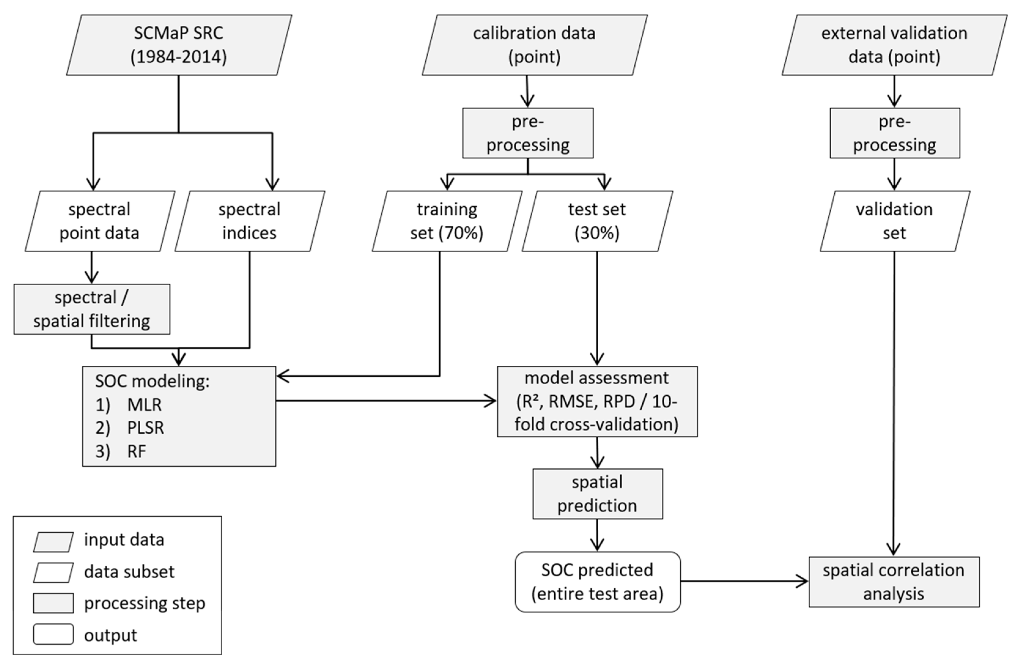
2. Materials and Methods
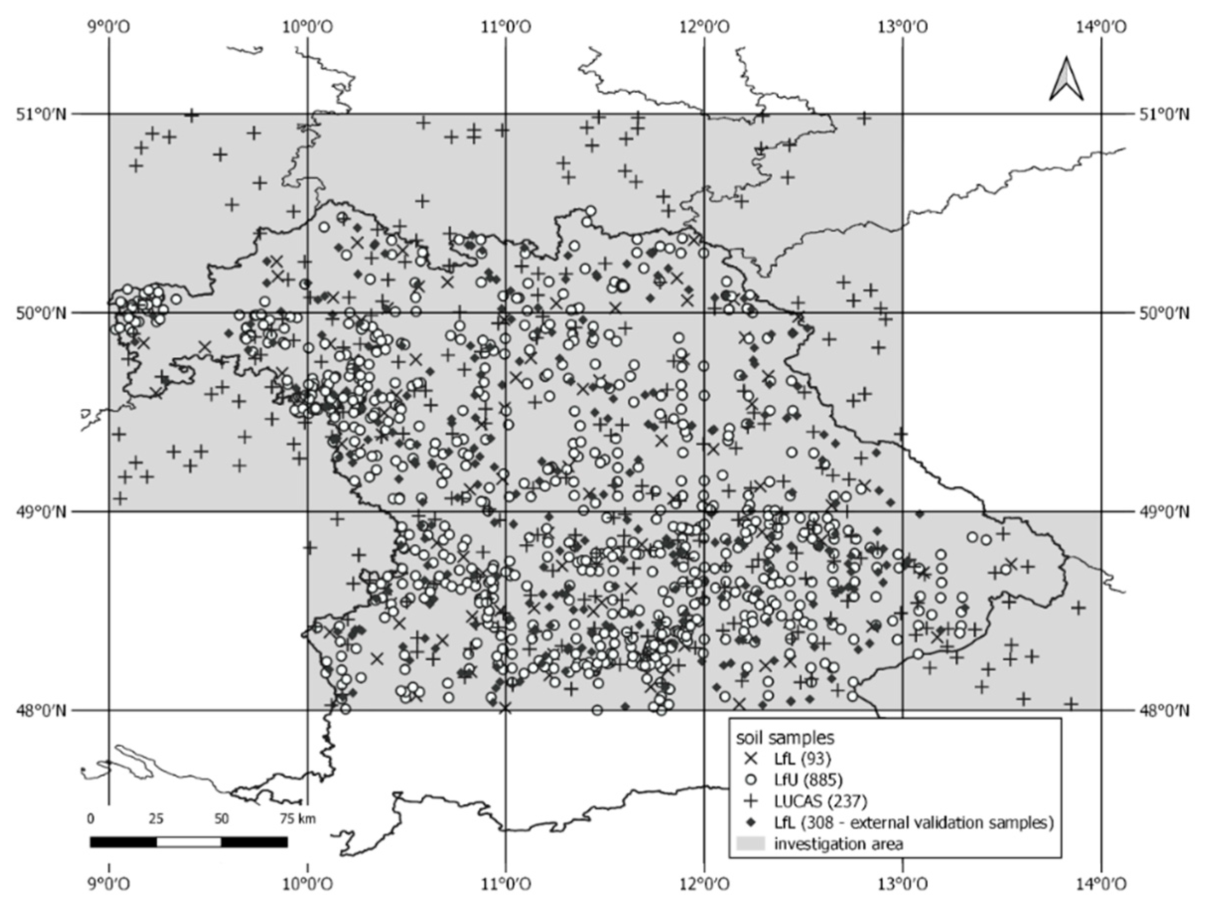
2.1. Study Area

The study area covers most of the Federal State of Bavaria (Figure 1) and adjacent regions in southeast Germany and was selected regarding the diversity of landscape and soil types. The area south of 48° N was excluded as permanent grassland is the dominating land use in this region, and SCMaP is not able to detect soils covered by permanent vegetation. Moreover, mountainous regions of the Alps in southern Bavaria were also excluded. Due to the frequent cloud coverage in this region, only a small number of cloudless scenes per pixel were available for the compositing process compared to other parts of Bavaria.
The study area comprises about 130,000 km², in which the elevation ranges between 100 m and 1000 m above sea level. The mean annual temperature lies between 6 °C and 10 °C, and the precipitation is between 551 mm and 1800 mm. The region is mainly dominated by Cambisols, Luvisols, Stagnosols, Gleysols and Leptosols [49] according to the World Reference Base for Soil Resource ([50]).

2.2. Soil Organic Carbon Modeling

An overview of the SOC modeling approach is outlined in Figure 2. Landsat 4–7 collection data from 1984 to 2014 are used to build the SRC based on the SCMaP workflow (Section 2.3). To calibrate an SOC model, SRC reflectance values and spectral indices (Section 2.3) are regressed against topsoil SOC measurements provided by two local authorities and the European LUCAS survey (Section 2.6).
Due to the positioning of several measurements at field borders, and thus, the potential integration of disturbances, a new filtering technique was developed and applied to evaluate the quality of calibration samples (Section 2.4). For the regression, three machine learning algorithms were tested and evaluated (Section 2.5). The models were trained for different datasets combining the reflectances and additional spectral indices.
Per algorithm, the best model is chosen, and the SOC contents are predicted for the entire study area. The prediction results are validated against external, independent SOC point measurements not included in the model calibration by a spatial correlation analysis (Section 2.7).

2.3. SCMaP SRC and Spectral Indices

The SCMaP chain [36] allows the generation of soil reflectance composites for individually determined time periods of different years. Bare soil pixels are selected based on a modified vegetation index (PV) using two thresholds that allow separating predominantly undisturbed soils from all other land cover types such as permanent vegetation and permanent non-vegetation. The derivation of the thresholds is based on an automated technique described in [51]. All selected bare soil pixels are averaged. The operational SCMaP chain can be used to build SRCs containing all pixels in a given time period showing at least once exposed soil.
For the SOC modeling, a period of 30 years (1984–2014) was chosen to provide a smooth spectral database that averages the seasonal variabilities of bare soils. The 30-year period was chosen for several reasons. A high possible soil coverage should be achieved. Using 5-year composites, 31.79% to 34.17% of the entire investigation area are selected as bare soil pixels. Ten-year composites provide 37.54% to 41.21% as exposed soils, and the 30-year composite enables the analysis of 54.53% of the investigation area as uncovered soils. Additionally, a possible large number of soil samples was intended to be used in the modeling dataset. A reduction of the compositing period would have significantly reduced the number of soil samples. For 5-year periods, 112 to 397 soil samples were collected in the respective periods. Based on 10-year composites, 261 to 536 samples are available. For a 30-year compositing range, 1,250 samples can be used for the modeling dataset. Additionally, an average over multiple years enables a reduction of seasonal soil moisture differences and permanent spatial differences remaining in the composite.
The SRC was processed for 228 Landsat-4 TM, 9,990 Landsat-5 ETM and 4,333 Landsat-7 ETM+ collection scenes [52] available between 1984 and 2014. For all scenes of all sensors, the same pre-processing steps were performed. The FMask algorithm [53,54] was used to detect and remove clouds, cloud shadows and pixels that were covered by snow. Additionally, an atmospheric correction was applied to all scenes using Atmospheric Topographic Correction (ATCOR) software for satellite imagery [55]. The quality of the composites is defined, among other factors, by the number of cloudless scenes per pixel [50]. The consistently large number of cloudless scenes per pixel for the total investigation time is given in Figure A1 in Appendix A.
In addition to the point spectral information of the SCMaP SRC, different indices were selected and computed (Table 2). Indices are commonly used in remote sensing to parameterize specific spectral features caused by physical and/or chemical properties [56]. Besides established indices, an additional index (SCMaPI) was developed to capture the difference between the green and the SWIR I bands of the SCMaP SRC. The SCMaPI shows smaller differences for high SOC content and higher differences for lower SOC content.

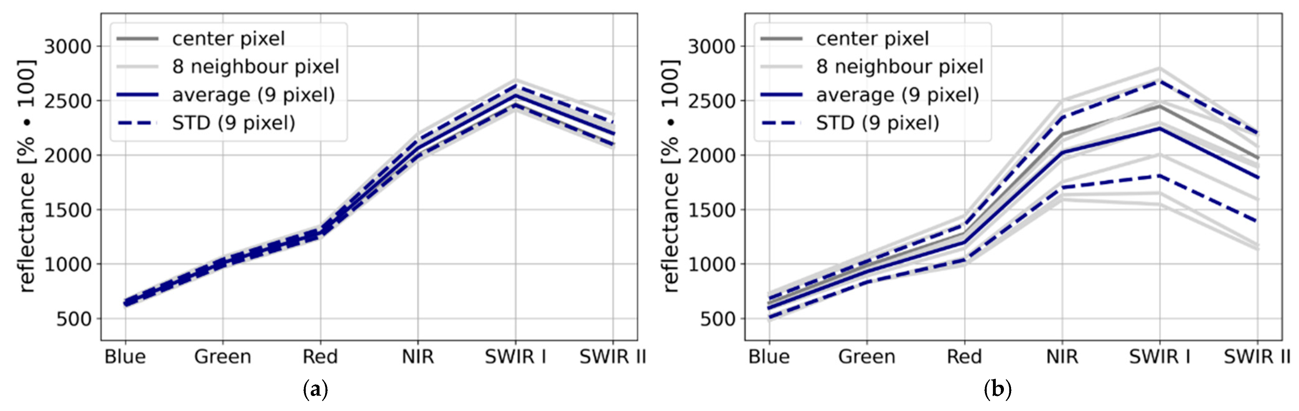
2.4. Spectral/Spatial Filtering Technique

Based on Landsat imagery, SCMaP provides soil reflectance information with a pixel resolution of 30 m. The link of a point soil sample to a 30 m pixel can result in inaccuracies if the soil sample is not collected at least 30 m from the field border. In this case, the SCMaP pixel may combine multiple surfaces with different spectral information, which are related to one soil sample. A proportion of the soil samples (especially the LUCAS points, [38]) are often taken within a few meters from the borders of agricultural fields, e.g., as shown by the photo documentation of the sampling points at the LUCAS viewer online (https://ec.europa.eu/eurostat/statistical-atlas/gis/viewer/?config=LUCAS-2009.json, accessed on 6 August 2021). The disturbance factors primarily exist at the field boundaries. Eliminating all samples that were collected within 30 m of the field border could decrease the number of biased pixels. However, this would drastically decrease the database and was therefore not considered. Instead, a spectral/spatial filtering technique was developed to prepare the soil database and the spectral information from the EO images for SOC modeling.
The filtering technique evaluates the spectral differences between the sample SRC pixel and its eight neighboring pixels. A comparison of the sample spectra to the neighboring pixel spectra allows an estimation if the reflectance spectra of the sample pixel are influenced by any external disturbances or data artefacts (e.g., mixed spectra of soil and a small portion of vegetation, local variation) or if they are comparable to the surrounding spectra. The spectral/spatial filtering aims to detect pixel clusters with deviating spectra to remove this from further processing. For this purpose, all STDs per pixel cluster per band were used to define a threshold to exclude the deviating pixel clusters. Twice, the STD per band of all pixel cluster STDs was selected as the threshold. The threshold was determined and applied per band. The identified pixel cluster containing at least one to several spectral bands above the thresholds was excluded from the dataset.

2.5. Soil Modeling Methods
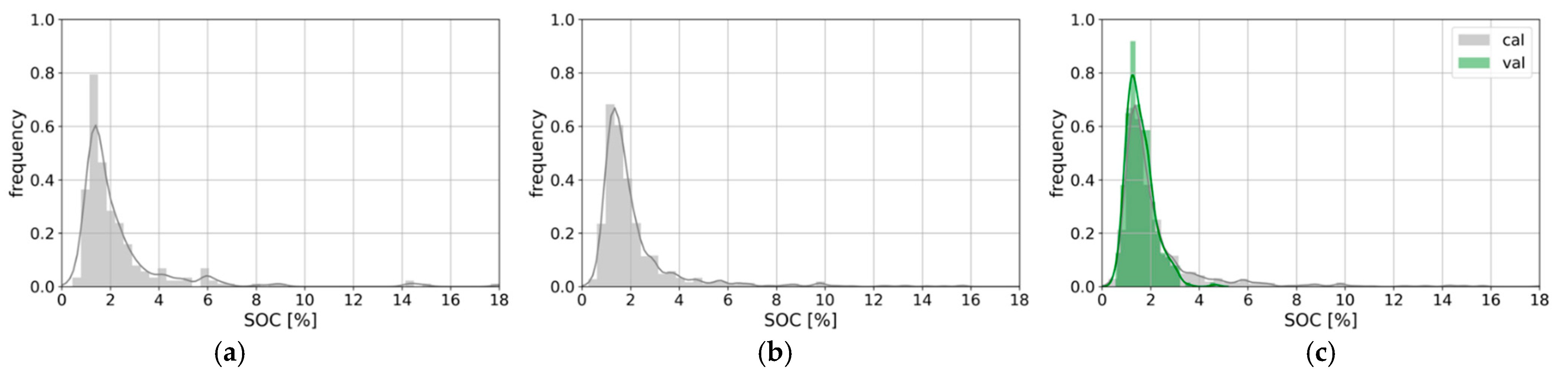
Three machine learning (ML) algorithms were used and evaluated. A Multiple Linear Regression (MLR), a Partial Least Square Regression (PLSR) [74] and a Random Forest regression (RF) algorithm [75] were applied to model the SOC contents in the topsoils. All three techniques are widely used in soil applications [76,77,78,79] and especially for SOC modeling (see Table 1, [22,23,37,39,40,41,42,43,44,45,46,47,48,49]). The modeling was performed using the Scikit-learn machine learning library for Python [80]. The following parameters were chosen for the RF: n_estimators: 100, max_features: 10, max_depth: 12, min_sample_split: 6, min_samples_leaf: 2 and for the PLSR: n_components: 5.
The calibration dataset was randomly split into a training (70%) and test (30%) subset. The training set was used to train the model, whereas the test subset of the calibration data was used to validate the model. For the model calibration and validation, common accuracy and performance measures, such as the R² (coefficient of determination, from sklearn.metrics), the root mean square error (RMSE) and the ratio of performance to deviation (RPD), were used to evaluate the model performances and to allow a comparison with the literature (Table 1). The RPD is an established performance measure that determines the quality of a model [81]. Moreover, the commonly used accuracy and performance measure, the Concordance Correlation Coefficient (CCC) [82], is given to assess the agreement between the predicted and measured SOC contents. Additionally, ten-fold cross-validation (cv) was performed to evaluate the performance of the models. The cv was applied to the training subset of the calibration data. In addition to the established accuracy and performance measures, an analysis of the standardized residuals and the autocorrelation of the residuals for the model calibration samples is given in Figure A2 and Figure A3 in the Appendix A.
Besides the reflectances, additional spectral indices (Table 2) per spectrally/spatially filtered sampling cluster were calculated and implemented in the modeling framework to investigate the influence of further spectral details. For this purpose, for each algorithm, three different model setups were prepared to estimate the influence of the spectral indices on the modeling capabilities. The models were trained based on (a) the composite reflectances (R), (b) the composite reflectances and all indices (RI_all) and (c) the composite reflectances and for each algorithm individually selected indices (RI_sel). Besides the reflectances and indices, no other covariates (e.g., clay content of climate variables) were used in the modeling framework.
For each algorithm, a selection of important features (RI_sel) was performed. The identification of the relevant features for the MLR was based on a linear correlation (Pearson’s correlation from Python sklearn.metrics). First, the relationship between the reflectances and indices to the modeling variable SOC was evaluated to exclude insignificant features (correlation coefficients (R) > 0.3). All significant feature pairs with correlation coefficients between −0.7 and 0.7 were then selected for the RI_sel dataset. For the PLSR, the variable importance in projection (VIP) per feature was calculated. Features with a VIP higher than 1.0 [22,83] were selected for the RI_sel dataset. For the RF, a calculation of the internal feature importance score (Mean Decrease Impurity (MDI)) was performed. Features with a score higher than 4.0% were selected as relevant features [84,85].
For each algorithm, the best model setup was selected regarding the cross-validation results and the model validation accuracies. For the best performance dataset (RI, RI_all, RI_sel), the models were applied to the 30-year SRC to predict the spatial SOC contents for the entire study area.

2.6. Soil Samples

For point SOC measurements, all available legacy data to cover the highest possible temporal and spatial overlap with the SRC between 1984 and 2014 were used. Kühnel et al. [86] found no significant OC changes between 1986 and 2015 of Bavarian croplands. The authors analyzed 92 repeatedly measured cropland sites in Bavaria. Therefore, all available sampling points between 1984 and 2014 were combined for the modeling dataset. However, there is a disadvantage of using legacy data, i.e., the sampling schemes are not optimally distributed.
The SOC measurements for the calibration set were provided by the Bavarian Environment Agency (LfU—1071 sampling sites) and the Bavarian State Research Center for Agriculture (LfL—134 sampling sites). Additionally, soil samples (504 sampling sites) collected in the framework of the LUCAS (Land Use/Cover Area frame statistical Survey) 2009 Topsoil Survey provided by the European Soil Data Centre (ESDAC) [87] were added (Figure 1). The LfU provided a large database with topsoil samples equally distributed across Bavaria [88]. The sites were each sampled once between 1984 and 2014. The LfL calibration dataset contained data from the permanent soil observation program (BDF) of Bavaria. In contrast to the once sampled LfU sites, these 134 BDFs were sampled multiple times in the observation period. As [86] found no significant change between 1986 and 2015 for the BDF sites across Bavaria, the available samples per BDF between 1984 and 2014 were averaged. Thus, one measurement per sampling location is included in the calibration dataset. The LUCAS soil samples were collected in 2009 from unique spatial positions across the investigation area. SOC contents of the LfU, LfL and LUCAS databases were all determined by dry combustion using elemental analyzers [88,89].
From all data sources, the samples intersecting with the SCMaP SRC and within the investigation period (1984 to 2014) were selected, i.e., 1385 soil samples. Per soil sample, the reflectance spectra and its eight neighboring pixels of the SRC were extracted and averaged to reduce local spatial variability. After the spectral/spatial filtering, 1215 sampling points for model calibration are remaining.
The external validation set was provided by the LfL and included 352 cropland fields with point SOC measurements sampled between 2001 and 2008. For each agricultural field, five sampling locations were randomly selected. At each sampling location (radius = 1.5 m), six soil samples were taken. SOC contents of all six soil samples of all five sampling locations were averaged to one SOC content per field. SOC contents were determined by dry combustions using CN elemental analyzers. For the external validation of the dataset, 308 samples were intersecting with the SCMaP SRC.
The data provided by the LfU contained the highest range of SOC contents (0.26% to 18.30%; Table 3). The LfL calibration data showed a lower mean SOC content in comparison to the LfU and LUCAS datasets. Overall, the calibration dataset contained locations with higher SOC contents compared to the external validation dataset.
For the model calibration and validation, the distribution of SOC contents of the training (70%) (Figure 3a) and test data (30%) (Figure 3b) were comparable. Both datasets contained samples with high SOC concentrations. The distribution of the SOC percentages of the calibration (cal) and the external independent validation (val) datasets (Figure 3c) showed a similar mean; however, the external validation dataset did not contain as high SOC concentrations.

2.7. External Validation

To evaluate the accuracy of the prediction models more precisely, a further validation was performed using an independent external dataset provided by LfL, which was not included in the training. For each regression algorithm, the best data set up based on the model accuracies and performance was selected and applied to predict the SOC contents for the entire investigation area. The difference for all samples between the predicted and measured SOC contents of the external independent validation dataset were calculated to estimate the averaged difference between the predicted and the measured contents to provide the reliability of predicting SOC for each algorithm.

3. Results

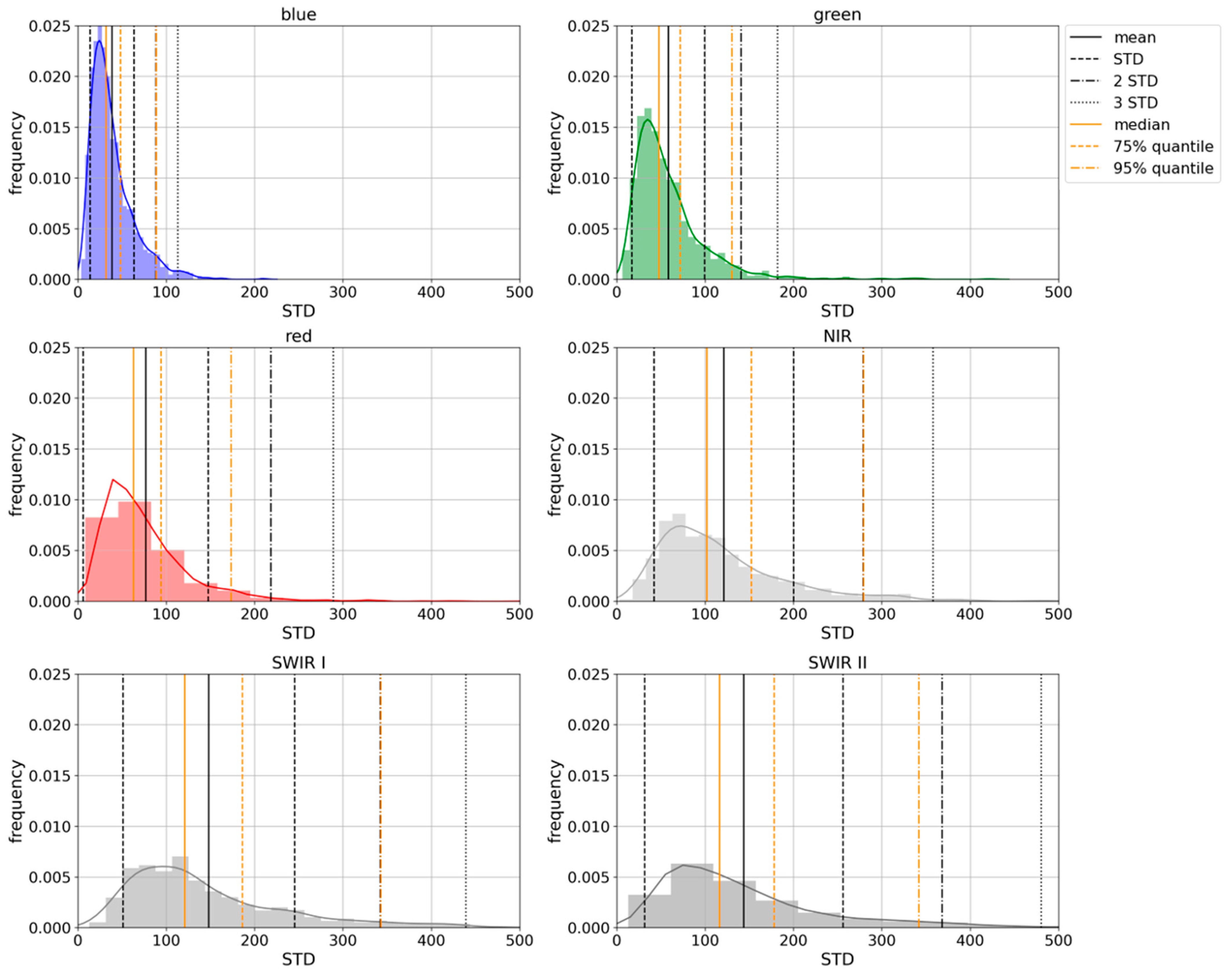
3.1. Spectral/Spatial Filtering

The spectral/spatial filtering was implemented in the model framework to ensure a high-quality calibration database. In order to ensure homogenous pixel clusters, a threshold is necessary to identify the heterogenous pixel clusters. Most of the nine individual pixel spectra per cluster showed homogenous patterns (Figure 4a). Here, an SOC measurement is linked to valid spectral information. However, a few pixel clusters showed deviating spectra (Figure 4b). These heterogenous pixel clusters with deviating individual spectra are represented by high standard deviations (STD) and need to be filtered, as here the possibility of any external influence or data artefacts (e.g., mixed spectra of soil and a small portion of vegetation, local variation) impacting the cluster is very high.
Figure 5 shows six histograms of all STDs per band for all sample clusters of the calibration dataset. As the threshold twice, the STD per band was selected to identify and eliminate the heterogenous clusters with deviating spectra. Overall, 135 pixel clusters (9.7% of the total calibration dataset) were eliminated from the calibration dataset. The pre-processed, spectrally/spatially filtered calibration set accordingly comprises 1250 averaged sampling clusters. As shown in Figure 5, using the STD as the threshold, a higher number of pixel clusters (674, 48.7%) are identified as heterogeneous clusters. However, a visual analysis showed that too many pixel clusters would be eliminated using the STD as the threshold. It was also tested to set the threshold at three-fold STD (3 STD). Although, this would result in an insufficient selection of heterogenous pixel clusters. A visual analysis has shown that the filtering of 50 pixel clusters (3.6%) selected by the three-fold STD threshold does not filter all heterogenous pixel clusters sufficiently.
The spatial/spectral filtering has a significant positive effect on the model accuracies. The RF was applied to the filtered and unfiltered RI_all datasets. A significant increase of the R² (0.64 to 0.67), a decrease of the RMSE (1.38% to 1.26%) and an increase of the RPD (1.46 to 1.56) indicated an improved performance of SOC modeling.

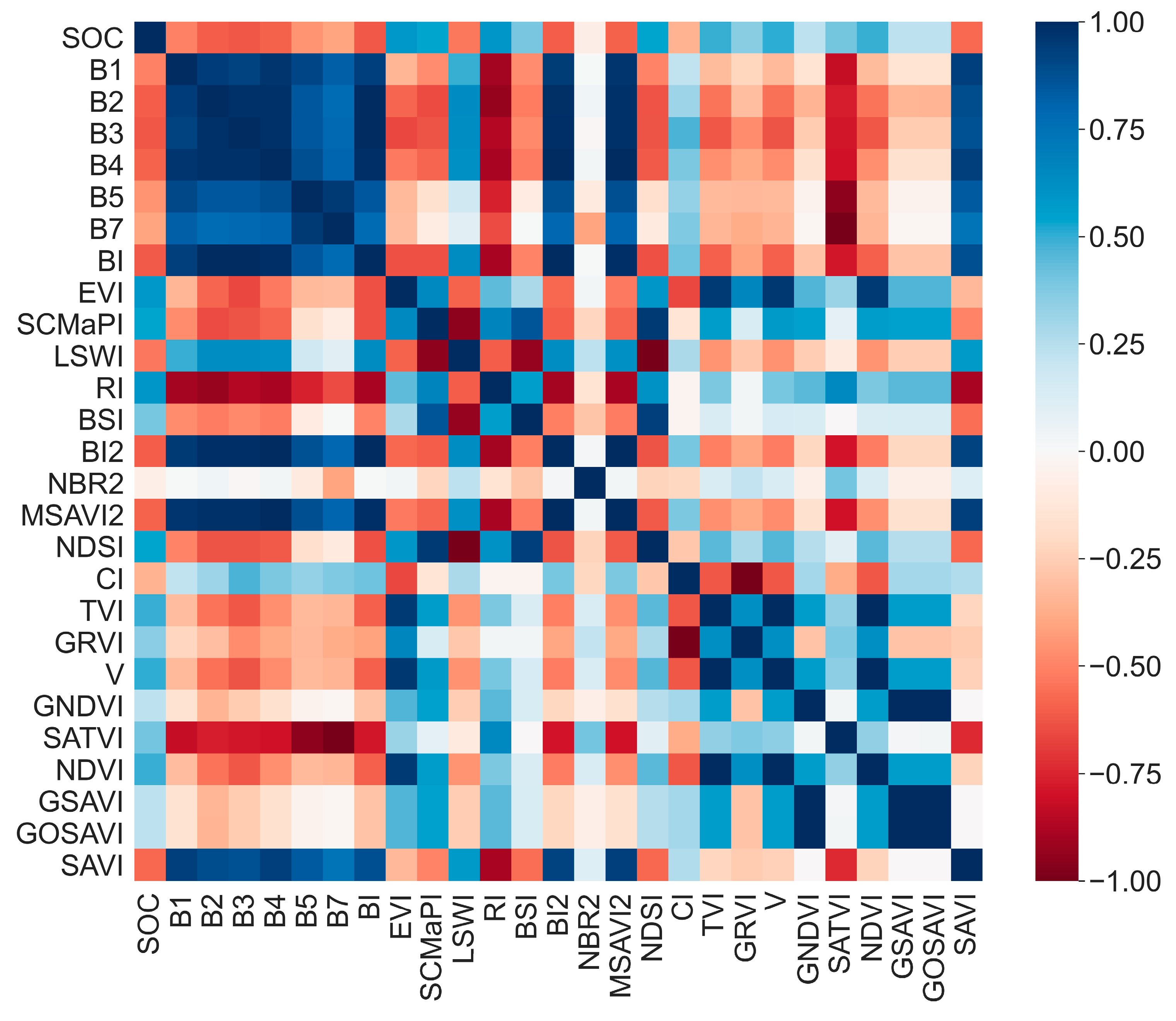
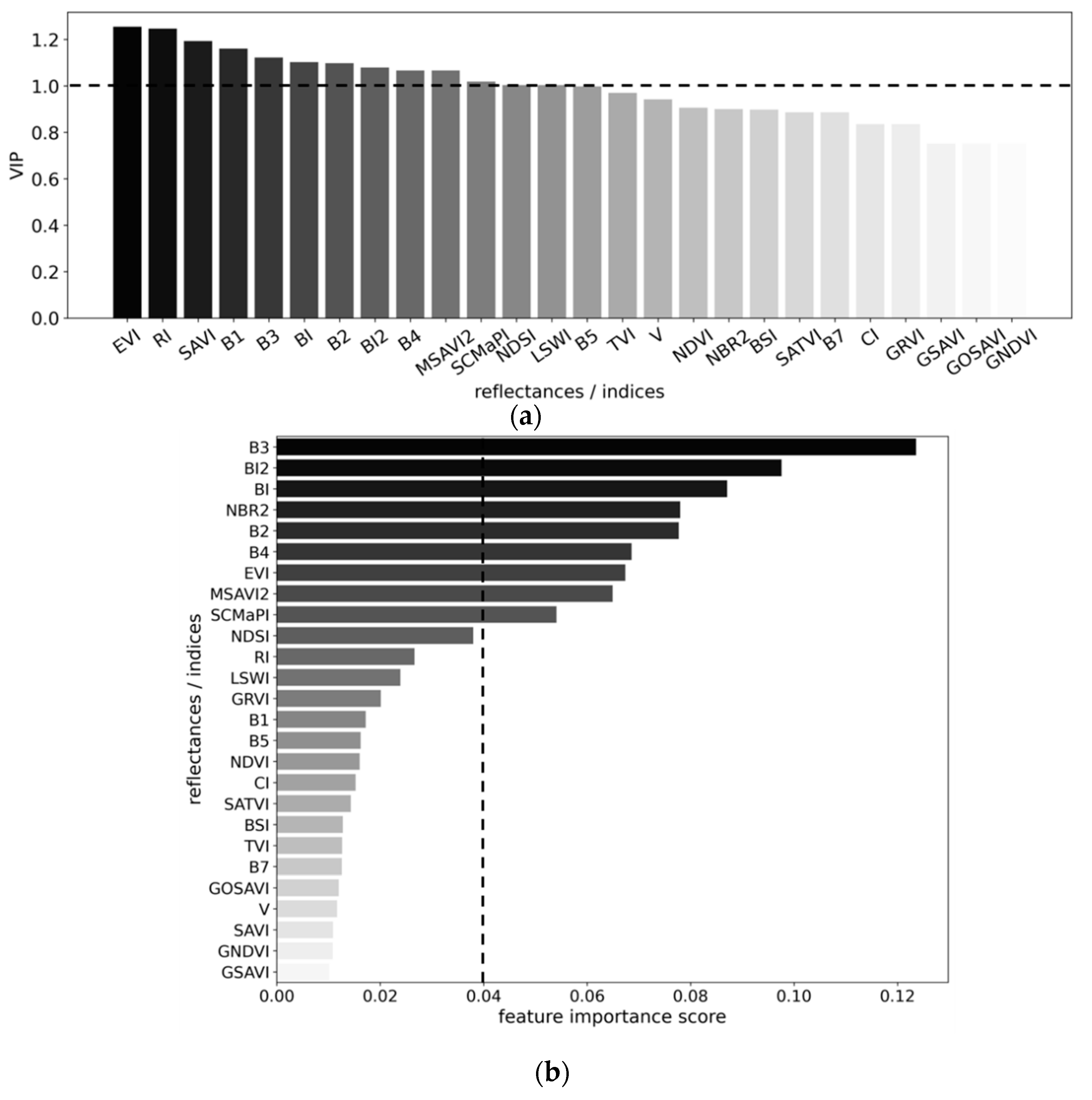
3.2. Feature Selection

For each ML algorithm, a feature selection was performed based on the correlation coefficients for the MLR (Figure 6), the VIP scores for the PLSR (Figure 7a) and the feature importance scores for the RF (Figure 7b). We selected 15 features for the MLR, 14 features for the PLSR, and 10 features for the RF. Overall, similar reflectance bands and indices were identified as important features for the individual RI_sel subsets. For the PLSR and the RF, the Landsat bands two (green), three (red) and four (near infrared—NIR) were selected as important features. For all three algorithms, the SCMaPI and the NDSI were selected, whereas the overlap of selected indices was higher for the PLSR and RF (Figure 7a,b). However, for the MLR, not all reflectance bands identified as significant features were flagged as independent features showing high R scores (>0.7) in the correlation matrix. This would result in an elimination of most of the reflectance bands. However, they were all included in the RI_sel database as the analysis of the SCMaP SRC reflectances is the focus of this study.

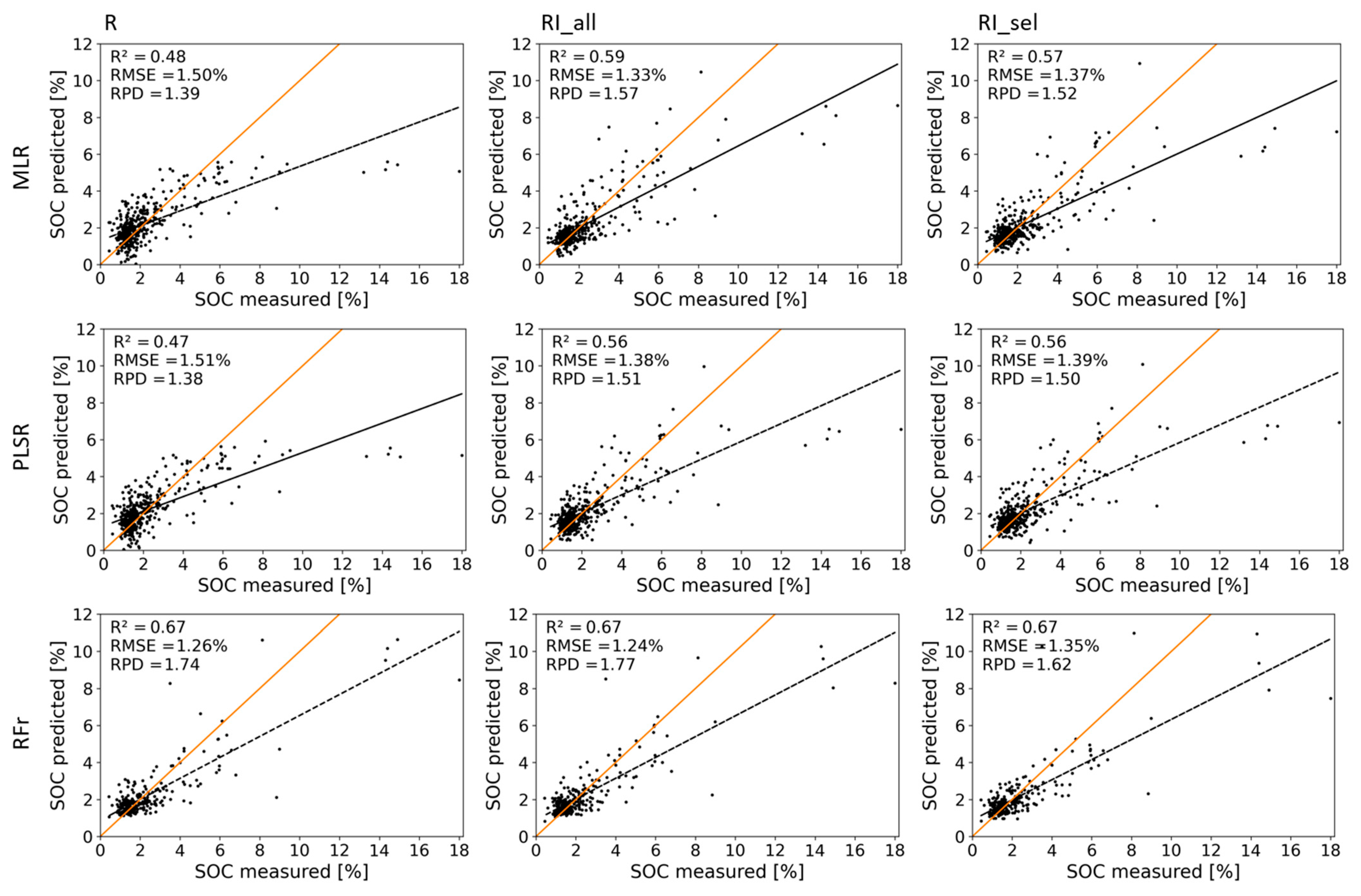
3.3. Model Results—Calibration

In order to ensure reliable models not overfitting the data, 10-fold cross-validation (cv) using 70% of the calibration data was additionally conducted to the model calibration using the same portion of data (Table 4). The remaining 30% of the calibration sampling points excluded from the model training were used for validating the models (Table 4, Figure 8).
The model accuracies and performances of the cv in comparison to the calibration results (cal) and validation results (val) are given in Table 4. Overall, except for minor differences for the RF similar R², RMSE and RPD values comparing the cal and cv results were detected for all datasets. This indicates that the cal models are valid and did not overfit the data. However, except for MLR and PLSR, based on the R datasets, the cv results are in a similar range compared to the val results. The model val results are in a similar range for the three algorithms. For PLSR and MLR, the use of additional indices is increasing the accuracies significantly. The influence of additional indices on the RF is less visible. Here, the R² is constant, the RPD is increasing, and the RMSE is decreasing. The RF shows the highest CCC values compared to the MLR and PLSR, whereas the CCC values for PLRS are lower based on the MLR.
Figure 8 shows the model validation results in detail for all three ML algorithms and for all prepared datasets. Overall, the RF regression performed best, showing the highest R² (0.67) and RPD scores (1.62 to 1.77) for the different datasets using the 30% validation sampling points of the calibration dataset. Based on RI_all, the best model accuracies comparing all datasets were obtained. The PLSR showed the lowest modeling accuracies with lower R² and RPDs and a higher RMSE in comparison to the other algorithms. The models based on the RI_all showed higher accuracies overall than the models based on the R data setup. The indices positively influenced the prediction of SOC. The RI_sel database showed no improvements in the model accuracies for the different ML algorithms. It is worth noting that for high SOC values, all regression approaches and all data set ups (reflectance and/or indices) underestimated the SOC.
Based on the cv and val results, the best set of features for all models was selected. For MLR, PLSR and RF, the model based on RI_all showed the best performances regarding the model validation and is therefore further used in this study. Using the RI_all feature set, the RF showed the best accuracies concerning the model training, cross validation and external validation.

3.4. External Validation

For each ML algorithm, the model based on the best feature subset was selected and applied to the whole investigation area. For each point of the external validation dataset, the predicted SOC contents were compared to the measured SOC values. Figure 9 shows the differences between the 308 pairs of values of the predicted and measured SOC contents for Figure 9a MLR (RI_all), Figure 9b PLSR (RI_all) and Figure 9c RF (RI_all). In total, the average errors were relatively low (0.11% ± 0.56% to 0.21% ± 0.61%) comparing the predicted and the measured values. The comparison of the predicted data based on the RF (RI_all) to the external validation data indicated the lowest mean difference. However, all three histograms showed a Gaussian-like distribution with a small number of outliers and a relatively small bias (mean and median values are close to 0.0 for all cases). The absolute differences ranged between −2.23% to +3.14% for MLR, −1.83% to 2.17% for PLSR and −2.56% to 3.05% for RF.

3.5. Spatial SOC Prediction

Overall, RF using the RI_all dataset provided the best model performance (R² = 0.67, RPD = 1.77), the highest model accuracy (RMSE = 1.24%) and the lowest mean difference comparing the predicted and the measured SOC contents of the independent external validation dataset (0.11% ± 0.56%). Consequently, the RF based on the RI_all dataset was applied to the whole study area. Figure 10 shows the spatial prediction results of the RF model.
Most of the study area revealed SOC contents lower than 2.0%, which is comparable to the mean SOC content of the soil datasets (Table 3). Regions with higher SOC contents (>6.0%) were mainly predicted in the South of Bavaria. Here, several patterns with relatively high SOC contents (>8.0%) are visible. High SOC contents are predicted in the river valleys in the south of the study area and in bogs and marshlands (e.g., Erdinger Moos around the Airport to the northeast of the city Munich or Königsmoos at the northeast of the city Augsburg). This is in line with an SOC map generated for Bavaria using a geostatistical modelling approach that showed the highest SOC stocks in floodplains and bogs [90].

4. Discussion

4.1. Spectral/Spatial Filtering

We applied spatial/spectral filtering to enable the link of a 30 m SRC pixel possibly influenced by different spectral information or other artefacts to a single point SOC measurement. The filtering is based on neighborhood relationships by evaluating the spectral information of the direct neighboring pixel in comparison to the spectral information of the sampling location. It is assumed that the soil sample is representative of the direct surrounding areas.
Due to the analysis of the STDs of all bands of all pixel clusters, all clusters with a heterogenous land cover were identified to be excluded from the input database due to their possible spectral influences. The spatial/spectral filtering has a significant positive effect on the model accuracies.
As shown in Figure 5, the distribution of the cluster STDs per reflectance band is representing a non-gaussian behavior, which indicates using the median and quantiles is more appropriate. Nevertheless, the selection of the threshold of the 2STD is equal to the 95% quantile for most bands. If the threshold is set using the 95% percentile, additionally six pixel clusters would be excluded and could provide an alternative to the presented method.
In general, the link between EO data with a pixel resolution of several meters and point soil samples provides a challenge for a wide variety of modeling purposes as point information is related to a larger area. The spectral/spatial filtering technique presented can help to identify, in particular, pixels that are not completely within a field boundary and therefore may contain a mixture of several spectral information (e.g., bare soil and vegetation at the edges of fields) for the sample point. As spectral neighborhood relationships of the pixel to which a soil sample is assigned are included in the assessment, the method can also be applied to other areas and is independent of any region or sensor-specific characteristics. The method shown is a simple and robust approach to exclude possibly disturbed pixels from the given data compilation. However, the applicability of the filtering technique has to be evaluated because it might not be best suited for larger or smaller pixel sizes. More suitable approaches that address the issue of linking point information to a pixel with the spatial extent of several meters should be explored.

4.2. Data and Modeling

In contrast to many other studies (Table 1), we used a bare soil composite consisting of a long time series of spaceborne Landsat imagery. Except for some case studies [25,37,43,48], all other models listed in Table 1 were built for single, cloudless multi- or hyperspectral scenes. In contrast, the SOC contents were predicted for a novel multispectral data source that was based on a large number of input scenes (14,061) for an area of nearly 130,000 km². Due to the long compositing period, all variabilities were included, and a stable mean SRC was provided. Small-scale spatial differences due to seasonal soil moisture differences are minimized. Soil moisture differences can have a huge influence on hyperspectral and multispectral remote sensing analysis and are addressed by several authors [91,92,93]. It hampers the prediction of soil variables from the reflectance spectra [94]. However, the influence of the permanent soil moisture differences regarding the used SRC has to be investigated.
For SOC modeling, three different ML algorithms were used and compared (Table 4, Figure 8). Overall, the RF showed the best model performances comparing the R² (0.62–0.67), RMSE (1.23–1.31), RPD values (1.62–1.77) and CCC results (0.78) for the model validation. However, the results of the RF and PLSR are comparable. Several indices were implemented in order to improve the SOC modeling capabilities. The application of indices is a widely used technique in remote sensing analyses and helps to capture more information, such as band ratios and spectral indices that are, e.g., sensitive to differences in soil properties [44]. As indicated by the model performance (Figure 8), an improvement can be noted for all three algorithms with the additional use of indices. However, the influence on MLR and PLSR was higher compared to the RF results. In this context, the additionally performed 10-fold cross-validation (Table 4) showed that a selection of relevant features is not necessarily required for the different ML algorithms. The PLSR and the RF results using RI_sel showed a small decrease in the model accuracies comparing the RI_all runs.
The model performances (Figure 8) based on the SCMaP SRC were comparable to the SOC prediction capabilities presented by various authors (Table 1). However, we covered a distinctly larger area (except for [25]) with a lower soil point density. However, in almost all studies, lower RMSE values were reported for the SOC prediction. The SOC content available for the study area shows a large range (0.26% to 18.3%; Table 3). A few of the referenced studies were based on a comparable distributed SOC data range. The high RMSEs could be related to the wide range of SOC content in the study area, as indicated by the general underestimation during the calibration stage for high SOC values (Figure 8). For analyzing the influence of high SOC content, it could be considered to separate organic soils with naturally high SOC contents from mineral soils with lower SOC content. A split of the soil samples regarding their SOC distribution was not considered as there was a small number of soil samples with higher SOC contents (52 samples; SOC content > 6%).
The SOC model performance based on the SCMaP SRC (RPD = 1.24, RMSE = 1.77) was slightly higher compared to the accuracies presented in Table 1 based on multitemporal Sentinel-2 (RPD = 1.4, RMSE = 0.34 [48], RPD = 1.06–1.68, RMSE = 0.209–0.363 [43], RPD = 0.99–1.53, RMSE = 0.253–0.545 [37]) or Landsat composites (RPD = 0.52–0.58, RMSE = 1.52–1.68 [25], RPD = 1.41, RMSE = 0.28 [48]). However, it must be emphasized that the RMSE’s shown are higher compared to the listed studies.
Using a 30-year composite could hamper the mapping of SOC contents if changes occur in the investigation area over time. However, for Bavaria, an analysis of SOC changes of the permanent soil observation sites in Bavaria showed a constant behavior of the SOC contents with relatively low overall changes between 1986 and 2016 [86]. Therefore, the use of a 30-year composite to overcome seasonal soil moisture differences is a reasonable approach to model SOC contents for large geographical areas where SOC changes are limited. Although, further analysis of the compositing technique to overcome seasonal soil moisture differences has to be conducted also with respect to the length of the compositing period. Additionally, for the investigation of SOC changes, the applicability of shorter compositing lengths has to be considered.

4.3. External Validation

In addition to the cross and model validation, we conducted an external validation based on an independent dataset. The predicted and measured SOC contents were compared, and the mean difference was calculated to estimate the accuracy of the modeling. The comparison showed small mean differences for MLR, PLSR and RF (0.11% to 0.21%). However, the SOC distribution of the validation dataset indicated small differences in comparison to the calibration dataset. The calibration dataset stretches between 0.26% and 18.3%, whereas the validation dataset contained samples with SOC contents between 0.55% and 4.65%. Although the majority of the calibration data is represented by the validation samples, very low (0.11% to 0.25%) and very high (4.66% to 18.3%) SOC contents are not included in the validation dataset. The comparison of the predicted SOC contents with the external validation dataset showed a small overestimation of the modeled SOC contents Figure 9, which has to be considered in the interpretation for the prediction of the entire study area (Figure 10).
To address large-scale SOC predictions (national to European-wide), further standardized validation datasets are needed. However, large-scale SOC maps are mostly available at a lower resolution (250 m to 1 km) and have limited suitability as a basis for validation for the 30 m pixel resolution of the SCMaP SRC database. A different aspect that could be considered for validation is an internal quality measure provided by the number of cloudless scenes per pixel. The usable data availability can be taken into consideration for data validation [51,95]. For the calibration and the validation dataset, an analysis of the number of cloudless observations of all sampling pixels showed a similar distribution (Figure 11a,b). On average, 300 scenes were available for the pixels of the SOC measurements. Both datasets showed a smaller peak on 200 scenes. These pixels are located in areas where the data of one Landsat path row is available. The absolute number of input scenes is smaller there. The smaller peak at 500 scenes per pixel can be related to overlapping areas, where several Landsat path rows are intersecting.
Figure 11c shows the link between the SOC differences and the distribution of cloudless scenes. The higher differences (<−2% and >2%) cannot be related to fewer cloudless scenes per pixel as the overall average of 300. These findings indicate that SCMaP captured the exposed soils well at the validation sampling points, and the influence of potentially remaining clouds is minimized and seems not to have any influence.

4.4. SCMaP SRC as Database for Modeling SOC Contents with High Spatial Resolution Covering Large Geographical Areas

In comparison to existing SOC maps (e.g., OCTOP [15], Topsoil Soil Organic Carbon Map based on the LUCAS Soil datasets for EU25 [16] or SoilGrids [96]), SCMaP provides a novel database for the estimation of soil parameters. The compositing approach allows the investigation of all areas which show at least once a bare soil within the observed time period. As the approach was trained using a large database and was successfully validated using independent data, the transferability to large-scale applications is feasible. In addition, high-resolution analysis considering within or between field differences is still possible as the original Landsat pixel size (30 m) is preserved (Figure 12).
As shown in Figure 10 and Figure 12, for several areas, relatively high SOC contents were predicted by the RF model. Here, a former peat bog (“Königsmoos”) is located, which naturally shows higher SOC contents. Such organic soils naturally contain higher SOC contents (>18.0 %) in comparison to other soils. Most of these peatlands have been drained for agricultural use [97].
A comparison with the soil map 1:200,000 (BUEK200, Federal Institute for Geosciences and Natural Resources, BGR) showed that areas with high predicted SOC contents are mostly fens, underpinning the correctness of the results. In addition, the qualitative SOC distributions shown in the study area are consistent with the results of SOC mapping in Bavaria shown in [90].

5. Conclusions

The potential of the SCMaP SRC database derived from Landsat images between 1984 and 2014 for large-scale applications with a high spatial resolution was evaluated. We used the SRC to model the spatial SOC distribution of exposed topsoils of croplands in Bavaria. The SRC was correlated with soil point measurements to quantify SOC contents for an area-wide mapping approach. We first developed a spatial/spectral filtering technique to address the challenge of linking a point soil sample to EO data with a pixel resolution of several meters. The results show that a spectral/spatial filtering of heterogenous pixel clusters is improving the SOC modeling.
For SOC quantification, several ML algorithms were applied and compared. The RF showed the highest capabilities to model the SOC content in Bavaria (R² = 0.67, RMSE = 1.24%, RPD = 1.77). Further, we determined that the use of additional spectral indices compared to the usage of reflectance data alone can improve SOC modeling.
In addition to the model validation based on a subset of the data, the best model setups (RI_all) were applied to the entire test area and validated using an external independent dataset (n = 308). The differences between the measured and predicted SOC contents were minor for all three ML algorithms and showed the lowest differences for the RF (0.11% ± 0.56% SOC).
The SCMaP SRC is a promising approach to predict the spatial SOC distribution for mapping a large geographical extent with high resolution at the farm or even the field scale. Nevertheless, for application on a larger scale, a validation approach has to be further developed. Several large-scale SOC products are available, although these maps are distributed on a lower resolution in comparison to the SCMaP capabilities.

Author Contributions

Conceptualization, S.Z. and U.H.; methodology, S.Z., M.B. and B.v.W.; software, S.Z. and M.B.; validation, S.Z., M.B. and M.W.; formal analysis, S.Z.; investigation, S.Z..; data curation, U.H. and S.Z.; writing—original draft preparation, S.Z.; writing—review and editing, S.Z., U.H., M.B., B.v.W., M.W. and M.S.; visualization, S.Z.; supervision, U.H. and B.v.W.; project administration, S.Z.; funding acquisition, U.H. All authors have read and agreed to the published version of the manuscript.

Funding

This research was funded by the German Federal Ministry of Food and Agriculture (BMEL), grant number 281B301816” as part of the Soil-DE Project “Entwicklung von Indikatoren zur Bewertung der Ertragsfähigkeit, Nutzungsintensität und Vulnerabilität landwirtschaftlich genutzter Böden in Deutschland”.

Institutional Review Board Statement

Not applicable.

Informed Consent Statement

Not applicable.

Data Availability Statement

Not applicable.

Acknowledgments

We thank the Bavarian agencies, the Bavarian Environment Agency (LfU) and the Bavarian State Research Center for Agriculture (LfL) for providing the soil databases.

Conflicts of Interest

The authors declare no conflict of interest.

Appendix A

Figure A1. The number of cloudless scenes per pixel for the total composite time (1984–2014) in the investigation area.
Remotesensing 13 03141 g0a1
Figure A2. Standardized residuals of the model validation (30% of data points).
Remotesensing 13 03141 g0a2
Figure A3. Autocorrelation of the prediction residuals of the model validation (30% of data points).
Remotesensing 13 03141 g0a3

References

  1. Lal, R.; Follett, R.F.; Stewart, B.A.; Kimble, J.M. Soil carbon sequestration to mitigate climate change and advance food security. Soil Sci. 2007, 172, 943–956. [Google Scholar] [CrossRef]
  2. Lehmann, J.; Hansel, C.M.; Kaiser, C.; Kleber, M.; Maher, K.; Manzoni, S.; Nunan, N.; Reichstein, M.; Schimel, J.P.; Torn, M.S. Persistence of Soil Organic Carbon Caused by Functional Complexity. Nat. Geosci. 2020, 13, 529–534. [Google Scholar] [CrossRef]
  3. Jobbágy, E.G.; Jackson, R.B. The vertical distribution of soil organic carbon and its relation to climate and vegetation. Ecol. Appl. 2000, 10, 423–436. [Google Scholar] [CrossRef]
  4. Scharlemann, J.P.; Tanner, E.V.; Hiederer, R.; Kapos, V. Global soil carbon: Understanding and managing the largest terrestrial carbon pool. Carbon Manag. 2014, 5, 81–91. [Google Scholar] [CrossRef]
  5. Wiesmeier, M.; Urbanski, L.; Hobley, E.; Lang, B.; von Lützow, M.; Marin-Spiotta, E.; van Wesemael, B.; Rabot, E.; Ließ, M.; Garcia-Franco, N. Soil organic carbon storage as a key function of soils—A review of drivers and indicators at various scales. Geoderma 2019, 333, 149–162. [Google Scholar] [CrossRef]
  6. Loveland, P.; Webb, J. Is there a critical level of organic mattes in the agricultural soils of temperate regions: A review. Soil Tillage Res. 2003, 70, 1–18. [Google Scholar] [CrossRef]
  7. Lal, R. Soil Health and carbon management. Food Energy Secur. 2016, 5, 212–222. [Google Scholar] [CrossRef]
  8. Gregorich, E.G.; Carter, M.R.; Angers, D.A.; Monreal, C.M.; Ellert, B. Towards a minimum data set to assess soil organic matter quality in agricultural soils. Can. J. Soil Sci. 1994, 74, 367–385. [Google Scholar] [CrossRef] [Green Version]
  9. Lal, R. Digging deeper: A holistic perspective of factors affecting soil organic carbon sequestration in agroecosystems. Glob. Chang. Biol. 2018, 24, 3285–3301. [Google Scholar] [CrossRef]
  10. Lorenz, K.; Lal, R.; Ehlers, K. Soil organic carbon stock as an indicator for monitoring land and soil degradation in relation to United Nations’ Sustainable Development Goals. Land Degrad. Dev. 2019, 30, 824–838. [Google Scholar] [CrossRef]
  11. Gollany, H.T.; Venterea, R.T. Measurements and models to identify agroecosystem practices that enhance soil organic carbon under changing climate. J. Environ. Qual. 2018, 47, 579–587. [Google Scholar] [CrossRef] [Green Version]
  12. Paustian, K.; Collier, S.; Baldock, J.; Burgess, R.; Creque, J.; DeLonge, M.; Dungait, J.; Ellert, B.; Frank, S.; Goddard, T.; et al. Quantifying carbon for agricultural soil management: From the current status toward a global soil information system. Carbon Manag. 2019, 10, 567–587. [Google Scholar] [CrossRef] [Green Version]
  13. Jandl, R.; Rodeghiero, M.; Martinez, C.; Cotrufo, M.F.; Bampa, F.; van Wesemael, B.; Harrison, R.B.; Guerrini, I.A.; Richter, D.D.; Rustad, L.; et al. Current status, uncertainty and future needs in soil organic carbon monitoring. Sci. Total. Environ. 2014, 468–469, 376–383. [Google Scholar] [CrossRef] [PubMed]
  14. Miller, B.A.; Schaetzl, R.J. The historical role of base maps in soil geography. Geoderma 2014, 230–231, 329–339. [Google Scholar] [CrossRef]
  15. Jones, R.J.A.; Hiederer, R.; Rusco, E.; Montanarella, L. Estimating organic carbon in the soils of Europe for policy support. Eur. J. Soil Sci. 2005, 56, 655–671. [Google Scholar] [CrossRef] [Green Version]
  16. de Brogniez, D.; Ballabio, C.; Stevens, A.; Jones, R.J.A.; Montanarella, L.; van Wesemael, B. A Map of the Topsoil Organic Carbon Content of Europe Generated by a Generalized Additive Model. Eur. J. Soil Sci. 2015, 66, 121–134. [Google Scholar] [CrossRef]
  17. Crucil, G.; Castaldi, F.; Aldana-Jague, E.; van Wesemael, B.; Macdonald, A.; Van Oost, K. Assessing the performance of UAS-compatible multispectral and hyperspectral sensors for soil organic carbon prediction. Sustainability 2019, 11, 1889. [Google Scholar] [CrossRef] [Green Version]
  18. Ben-Dor, E.; Chabrillat, S.; Demattê, J.A.M.; Taylor, G.R.; Hill, J.; Whiting, M.L.; Sommer, S. Using imaging spectroscopy to study soil properties. Remote. Sens. Environ. 2009, 113, S38–S55. [Google Scholar] [CrossRef]
  19. Bartholomeus, H.; Kooistra, L.; Stevens, A.; van Leeuwen, M.; van Wesemael, B.; Ben-Dor, E.; Tychon, B. Soil organic carbon mapping of partially vegetated agricultural fields with imaging spectroscopy. Int. J. Appl. Earth Obs. Geoinf. 2011, 13, 81–88. [Google Scholar] [CrossRef]
  20. Bayer, A.D.; Bachmann, M.; Rogge, D.; Muller, A.; Kaufmann, H. Combining field and imaging spectroscopy to map soil organic carbon in a semiarid environment. IEEE J. Sel. Top. Appl. Earth Obs. Remote. Sens. 2016, 9, 3997–4010. [Google Scholar] [CrossRef]
  21. Chabrillat, S.; Ben-Dor, E.; Cierniewski, J.; Gomez, C.; Schmid, T.; van Wesemael, B. Imaging spectroscopy for soil mapping and monitoring. Surv. Geophys. 2019, 40, 361–399. [Google Scholar] [CrossRef] [Green Version]
  22. Castaldi, F.; Hueni, A.; Chabrillat, S.; Ward, K.; Buttafuoco, G.; Bomans, B.; Vreys, K.; Brell, M.; van Wesemael, B. Evaluating the capability of the Sentinel 2 data for soil organic carbon prediction in croplands. ISPRS J. Photogramm. Remote. Sens. 2019, 147, 267–282. [Google Scholar] [CrossRef]
  23. Vaudour, E.; Gomez, C.; Fouad, Y.; Lagacherie, P. Sentinel-2 image capacities to predict common topsoil properties of temperate and Mediterranean agroecosystems. Remote. Sens. Environ. 2019, 223, 21–33. [Google Scholar] [CrossRef]
  24. Wang, X.; Zhang, Y.; Atkinson, P.M.; Yao, H. Predicting soil organic carbon content in Spain by combining landsat TM and ALOS PALSAR images. Int. J. Appl. Earth Obs. Geoinf. 2020, 92, 102182. [Google Scholar] [CrossRef]
  25. Safanelli, J.L.; Chabrillat, S.; Ben-Dor, E.; Demattê, J.A.M. Multispectral models from bare soil composites for mapping topsoil properties over Europe. Remote Sens. 2020, 12, 1369. [Google Scholar] [CrossRef]
  26. Diek, S.; Fornallaz, F.; Schaepman, M.E.; De Jong, R. Barest pixel composite for agricultural areas using Landsat time series. Remote Sens. 2017, 9, 1245. [Google Scholar] [CrossRef] [Green Version]
  27. Demattê, J.A.M.; Fongaro, C.T.; Rizzo, R.; Safanelli, J.L. Geospatial Soil Sensing System (GEOS3): A powerful data mining procedure to retrieve soil spectral reflectance from satellite images. Remote Sens. Environ. 2018, 212, 161–175. [Google Scholar] [CrossRef]
  28. Demattê, J.A.M.; Safanelli, J.L.; Poppiel, R.R.; Rizzo, R.; Silvero, N.E.Q.; de Sousa Mendes, W.; Bonfatti, B.R.; Dotto, A.C.; Salazar, D.F.U.; de Oliveira Mello, F.A.; et al. Bare Earth’s surface spectra as a proxy for soil resource monitoring. Sci. Rep. 2020, 10, 4461. [Google Scholar] [CrossRef] [PubMed]
  29. Hansen, M.C.; Egorov, A.; Roy, D.P.; Potapov, P.; Ju, J.; Turubanova, S.; Kommareddy, I.; Loveland, T.R. Continuous fields of land cover for the conterminous United States using Landsat data: First results from the Web-Enabled Landsat Data (WELD) project. Remote Sens. Lett. 2011, 2, 279–288. [Google Scholar] [CrossRef]
  30. White, J.C.; Wulder, M.A.; Hobart, G.W.; Luther, J.E.; Hermosilla, T.; Griffiths, P.; Coops, N.C.; Hall, R.J.; Hostert, P.; Dyk, A.; et al. Pixel-based image compositing for large-area dense time series applications and science. Can. J. Remote Sens. 2014, 40, 192–212. [Google Scholar] [CrossRef] [Green Version]
  31. Hermosilla, T.; Wulder, M.A.; White, J.C.; Coops, N.C.; Hobart, G.W. An integrated Landsat time series protocol for change detection and generation of annual gap-free surface reflectance composites. Remote. Sens. Environ. 2015, 158, 220–234. [Google Scholar] [CrossRef]
  32. Griffiths, P.; Nendel, C.; Hostert, P. Intra-annual reflectance composites from Sentinel-2 and Landsat for national-scale crop and land cover mapping. Remote Sens. Environ. 2019, 220, 135–151. [Google Scholar] [CrossRef]
  33. Loiseau, T.; Chen, S.; Mulder, V.L.; Dobarco, M.R.; Richer-de-Forges, A.C.; Lehmann, S.; Bourennane, H.; Saby, N.P.; Martin, M.P.; Vaudour, E. Satellite data integration for soil clay content modelling at a national scale. Int. J. Appl. Earth Obs. Geoinf. 2019, 82, 101905. [Google Scholar] [CrossRef]
  34. Adams, B.; Iverson, L.; Matthews, S.; Peters, M.; Prasad, A.; Hix, D.M. Mapping forest composition with Landsat time series: An evaluation of seasonal composites and harmonic regression. Remote Sens. 2020, 12, 610. [Google Scholar] [CrossRef] [Green Version]
  35. Wulder, M.A.; White, J.C.; Loveland, T.R.; Woodcock, C.E.; Belward, A.S.; Cohen, W.B.; Fosnight, E.A.; Shaw, J.; Masek, J.G.; Roy, D.P. The global Landsat archive: Status, consolidation, and direction. Remote Sens. Environ. 2016, 185, 271–283. [Google Scholar] [CrossRef] [Green Version]
  36. Rogge, D.; Bauer, A.; Zeidler, J.; Mueller, A.; Esch, T.; Heiden, U. Building an exposed soil composite processor (SCMaP) for mapping spatial and temporal characteristics of soils with Landsat imagery (1984–2014). Remote. Sens. Environ. 2018, 205, 1–17. [Google Scholar] [CrossRef] [Green Version]
  37. Vaudour, E.; Fomez, C.; Lagacherie, P.; Loiseau, T.; Baghdadi, N.; Urbina-Salazar, D.; Loubet, B.; Arrouays, D. Temporal mosaicking approaches of Sentinel-2 images for extending organic carbon content mapping in croplands. Int. J. Appl. Earth Obs. Geoinf. 2021, 96, 102277. [Google Scholar] [CrossRef]
  38. Weigand, M.; Staab, J.; Wurm, M.; Taubenböck, H. Spatial and semantic effects of LUCAS samples on fully automated land use/land cover classification in high-resolution Sentinel-2 data. Int. J. Appl. Earth Obs. Geoinf. 2020, 88, 102065. [Google Scholar] [CrossRef]
  39. Castaldi, F.; Palombi, A.; Santini, F.; Pascucci, S.; Pignatti, S.; Casa, R. Evaludation of the potential of the current and forthcoming multispectral and hyperspectral imagers to estimate soil texture and organic carbon. Remote Sens. Environ. 2016, 179, 54–65. [Google Scholar] [CrossRef]
  40. Castaldi, F.; Chabrillat, S.; Jones, A.; Vreys, K.; Bomans, B.; van Wesemael, B. Soil organic carbon estimation in croplands by hyperspectral remote APEX data using the LUCAS topsoil database. Remote Sens. 2018, 10, 153. [Google Scholar] [CrossRef] [Green Version]
  41. Castaldi, F.; Chabrillat, S.; Don, A.; van Wesemael, B. Soil organic carbon mapping using LUCAS topsoil database and Sentinel-2 data: An approach to reduce soil moisture and crop residue effects. Remote Sens. 2019, 11, 2121. [Google Scholar] [CrossRef] [Green Version]
  42. Castaldi, F.; Chabrillat, S.; van Wesemael, B. Sampling strategies for soil property mapping using multispectral Sentinel-2 and hyperspectral EnMAP satellite data. Remote Sens. 2019, 11, 309. [Google Scholar] [CrossRef] [Green Version]
  43. Dvorakova, K.; Heiden, U.; van Wesemael, B. Sentinel-2 exposed soil composite for soil organic carbon prediction. Remote Sens. 2021, 13, 1791. [Google Scholar] [CrossRef]
  44. Gholizadeh, A.; Žižala, D.; Saberioon, M.; Borůvka, L. Soil organic carbon and texture retrieving and mapping using proximal, airborne and Sentinel-2 spectral imaging. Remote Sens. Environ. 2018, 218, 89–103. [Google Scholar] [CrossRef]
  45. Hbirkou, C.; Pätzold, S.; Mahlein, A.-K.; Welp, G. Airborne hyperspectral imaging of spatial soil organic carbon heterogeneity at the field-scale. Geoderma 2012, 175–176, 21–28. [Google Scholar] [CrossRef]
  46. Selige, T.; Böhner, J.; Schmidhalter, U. High resolution topsoil mapping using hyperspectral image and field data in multivariate regression modeling procedures. Geoderma 2006, 136, 235–244. [Google Scholar] [CrossRef]
  47. Vaudour, E.; Gomez, C.; Loiseau, T.; Baghdadi, N.; Loubet, B.; Arrouays, D.; Ali, L.; Lagacherie, P. The impact of acquisition date on the prediction performance of topsoil organic carbon from Sentinel-2 for croplands. Remote Sens. 2019, 11, 2143. [Google Scholar] [CrossRef] [Green Version]
  48. Žížala, D.; Minařík, R.; Zádorová, T. Soil organic carbon mapping using multispectral remote sensing data: Prediction ability of data with different spatial and spectral resolutions. Remote Sens. 2019, 11, 2947. [Google Scholar] [CrossRef]
  49. Wiesmeier, M.; Hübner, R.; Barthold, F.; Spörlein, P.; Geuß, U.; Hangen, E.; Reischl, A.; Schilling, B.; von Lützow, M.; Kögel-Knabner, I. Amount, distribution and driving factors of soil organic carbon and nitrogen in cropland and grassland soils of Southeast Germany (Bavaria). Agric. Ecosyst. Environ. 2013, 176, 39–52. [Google Scholar] [CrossRef]
  50. Wrb, I.W.G. World reference base for soil resources 2015. World Soil Resour. Rep. 2015, 103, 128. [Google Scholar]
  51. Zepp, S.; Jilge, M.; Metz-Marconcini, A.; Heiden, U. The influence of vegetation index thresholding on EO-based assessments of exposed soil masks in Germany between 1984 and 2019. ISPRS J. Photogramm. Remote. Sens. 2021, 178, 366–381. [Google Scholar] [CrossRef]
  52. Wulder, M.A.; Loveland, T.R.; Roy, D.P.; Crawford, C.J.; Masek, J.G.; Woodcock, C.E.; Allen, R.G.; Anderson, M.C.; Belward, A.S.; Cohen, W.B.; et al. Current status of Landsat program, science, and applications. Remote Sens. Environ. 2019, 225, 127–147. [Google Scholar] [CrossRef]
  53. Zhu, Z.; Woodcock, C.E. Object-based cloud and cloud shadow detection in Landsat imagery. Remote Sens. Environ. 2012, 118, 89–98. [Google Scholar] [CrossRef]
  54. Zhu, Z.; Wang, S.; Woodcock, C.E. Improvement and expansion of the Fmask algorithm: Cloud, cloud shadow, and snow detectionn for Landsat 4-7, 8 and Sentinel-2 images. Remote Sens. Environ. 2015, 159, 269–277. [Google Scholar] [CrossRef]
  55. Richter, R.; Schläpfer, D. Atmospheric/Topographic Correction for Satellite Imagery/ATCOR-2/3 User Guide, Version 8.3.1; ReSe Applications Schläpfer Langeggweg: Wil, Switzerland, 2014; Volume 3. [Google Scholar]
  56. Van Deventer, A.P.; Ward, A.D.; Gowda, P.H.; Lyon, J.G. Using thematic mapper data to identify contrasting soil plains and tillage practices. Photogramm. Eng. Remote Sens. 1997, 63, 87–93. [Google Scholar]
  57. Escadafal, R. Remote sensing of arid soil surface color with Landsat thematic mapper. Adv. Space Res. 1989, 9, 159–163. [Google Scholar] [CrossRef]
  58. Huete, A.; Didan, K.; Miura, T.; Rodriguez, E.P.; Gao, X.; Ferreira, L.G. Overview of the radiometric and biophysical performance of the MODIS vegetation indices. Remote Sens. Environ. 2002, 83, 195–213. [Google Scholar] [CrossRef]
  59. Key, C.H.; Benson, N.C. Landscape Assessment (LA). In FIREMON: Fire Effects Monitoring and Inventory System; Gen. Tech. Rep. RMRS-GTR-164-CD; Lutes, D.C., Keane, R.E., Caratti, J.F., Key, C.H., Benson, N.C., Sutherland, S., Gangi, L.J., Eds.; US Department of Agriculture, Forest Service, Rocky Mountain Research Station: Fort Collins, CO, USA, 2006; p. LA-1-55 2006, 164. [Google Scholar]
  60. Qi, J.; Kerr, Y.; Chehbouni, A. External factor consideration in vegetation index development. Proc. Phys. Meas. Signat. Remote Sens. ISPRS 1994, 723, 730. [Google Scholar]
  61. Xiao, X.; Zhang, Q.; Braswell, B.; Urbanski, S.; Boles, S.; Wofsy, S.; Moore III, B.; Ojima, D. Modeling gross primary production of temperate deciduous broadleaf forest using satellite images and climate data. Remote Sens. Environ. 2004, 91, 256–270. [Google Scholar] [CrossRef]
  62. Rogers, A.S.; Kearney, M.S. Reducing signature variability in unmixing coastal marsh thematic mapper scenes using spectral indices. Int. J. Remote. Sens. 2004, 25, 2317–2335. [Google Scholar] [CrossRef]
  63. Pouget, M.; Madeira, J.; Le Floch, E.; Kamal, S. Caracteristiques spectrales des surfaces sableuses de la Region Cotiere Nord-Ouest de l’Egypte. Appl. Aux Donnees Satell. SPOT 1990, 4–6. [Google Scholar]
  64. Chen, W.; Liu, L.; Zhang, C.; Wang, J.; Wang, J.; Pan, Y. Monitoring the seasonal bare soil areas in Beijing using multitemporal TM images. In Proceedings of the IGARSS 2004. 2004 IEEE International Geoscience and Remote Sensing Symposium, Anchorage, AK, USA, 20–24 September 2004; Volume 5, pp. 3379–3382. [Google Scholar]
  65. Nellis, M.D.; Briggs, J.M. Transformed vegetation index for measuring spatial variation in drought impacted biomass on Konza Prairie, Kansas. Trans. Kans. Acad. Sci. 1992, 95, 93. [Google Scholar] [CrossRef]
  66. Tucker, C.J. Red and photographic infrared linear combinations for monitoring vegetation. Remote Sens. Environ. 1979, 8, 127–150. [Google Scholar] [CrossRef] [Green Version]
  67. Jordan, C.F. Derivation of leaf-area index from quality of light on the forest floor. Ecology 1969, 50, 663–666. [Google Scholar] [CrossRef]
  68. Gitelson, A.A.; Kaufman, Y.J.; Merzlyak, M.N. Use of a green channel in remote sensing of global vegetation from EOS-MODIS. Remote Sens. Environ. 1996, 58, 289–298. [Google Scholar] [CrossRef]
  69. Marsett, R.C.; Qi, J.; Heilman, P.; Biedenbender, S.H.; Watson, M.C.; Amer, S.; Weltz, M.; Goodrich, D.; Marsett, R. Remote sensing for grassland management in the arid southwest. Rangel. Ecol. Manag. 2006, 59, 530–540. [Google Scholar] [CrossRef]
  70. Rouse, J.W.; Haas, R.H.; Schell, J.A.; Deering, D.W. Monitoring vegetation systems in the great plains with ERTS proceeding. In Proceedings of the Third Earth Reserves Technology Satellite Symposium, Washington, DC, USA, 10–14 December 1973; Volume 30103017. [Google Scholar]
  71. Tian, Y.; Yan, Z.; Weixing, C. Monitoring soluble sugar, total nitrogen & its ratio in wheat leaves with canopy spectral reflectance. Zuo Wu Xue Bao 2005, 31, 355–360. [Google Scholar]
  72. Rondeaux, G.; Steven, M.; Baret, F. Optimization of soil-adjusted vegetation indices. Remote Sens. Environ. 1996, 55, 95–107. [Google Scholar] [CrossRef]
  73. Huete, A.; Huete, A.R. A Soil-Adjusted Vegetation Index (SAVI). Remote Sens. Environ. 1988, 25, 295–309. [Google Scholar] [CrossRef]
  74. Wold, S.; Sjöström, M.; Eriksson, L. PLS-Regression: A basic tool of chemometrics. Chemom. Intell. Lab. Syst. 2001, 58, 109–130. [Google Scholar] [CrossRef]
  75. Breiman, L. Random forests. Mach. Learn. 2001, 45, 5–32. [Google Scholar] [CrossRef] [Green Version]
  76. da Silva Chagas, C.; de Carvalho Junior, W.; Bhering, S.B.; Calderano Filho, B. Spatial prediction of soil surface texture in a semiarid region using random forest and multiple linear regressions. Catena 2016, 139, 232–240. [Google Scholar] [CrossRef]
  77. Jiang, Q.; Chen, Y.; Guo, L.; Fei, T.; Qi, K. Estimating soil organic carbon of cropland soil at different levels of soil moisture using VIS-NIR spectroscopy. Remote Sens. 2016, 8, 755. [Google Scholar] [CrossRef] [Green Version]
  78. Ward, K.J.; Chabrillat, S.; Neumann, C.; Foerster, S. A remote sensing adapted approach for soil organic carbon prediction based on the spectrally clustered LUCAS soil database. Geoderma 2019, 353, 297–307. [Google Scholar] [CrossRef]
  79. Xie, X.; Wu, T.; Zhu, M.; Jiang, G.; Xu, Y.; Wang, X.; Pu, L. Comparison of random forest and multiple linear regression models for estimation of soil extracellular enzyme activities in agricultural reclaimed coastal saline land. Ecol. Indic. 2021, 120, 106925. [Google Scholar] [CrossRef]
  80. Pedregosa, F.; Varoquaux, G.; Gramfort, A.; Michel, V.; Thirion, B.; Grisel, O.; Blondel, M.; Prettenhofer, P.; Weiss, R.; Dubourg, V. Scikit-learn: Machine learning in python. J. Mach. Learn. Res. 2011, 12, 2825–2830. [Google Scholar]
  81. Chang, C.-W.; Laird, D.A. Near-infrared reflectance spectroscopic analysis of soil C and N. Soil Sci. 2002, 167, 110–116. [Google Scholar] [CrossRef]
  82. Lin, L.I.-K. A Concordance correlation coefficient to evaluate reproducibility. Biometrics 1989, 45, 255–268. [Google Scholar] [CrossRef] [PubMed]
  83. Chong, I.-G.; Jun, C.-H. Performance of some variable selection methods when multicollinearity is present. Chemom. Intell. Lab. Syst. 2005, 78, 103–122. [Google Scholar] [CrossRef]
  84. Hobley, E.; Wilson, B.; Wilkie, A.; Gray, J.; Koen, T. Drivers of soil organic carbon storage and vertical distribution in Eastern Australie. Plant. Soil 2015, 390, 111–127. [Google Scholar] [CrossRef]
  85. Hobley, E.U.; Baldock, J.; Wilson, B. Environmental and human influences on organic carbon fractions down the soil profile. Agric. Ecosyst. Environ. 2016, 223, 152–166. [Google Scholar] [CrossRef] [Green Version]
  86. Kühnel, A.; Wiesmeier, M.; Kögel-Knabner, I.; Spörlein, P. Veränderungen der Humusqualität und -Quantität Bayerischer Böden im Klimawandel; Umwelt Spezial; Bayerisches Landesamt für Umwelt: Hof, Germany, 2020. [Google Scholar]
  87. Tóth, G.; Jones, A.; Montanarella, L. LUCAS Topsoil Survey: Methodology, Data and Results; Publications Office: Luxembourg, 2013; ISBN 92-79-32542-6. [Google Scholar]
  88. Wiesmeier, M.; Spörlein, P.; Geuß, U.W.E.; Hangen, E.; Haug, S.; Reischl, A.; Schilling, B.; von Lützow, M.; Kögel-Knabner, I. Soil organic carbon stocks in Southeast Germany (Bavaria) as affected by land use, soil type and sampling depth. Glob. Chang. Biol. 2012, 18, 2233–2245. [Google Scholar] [CrossRef]
  89. Origazzi, A.; Ballabio, C.; Panagos, P.; Jones, A.; Fernández-Ugalde, O. LUCAS soil, the largest expandable soil dataset for Europe: A review. Eur. J. Soil Sci. 2018, 69, 140–153. [Google Scholar] [CrossRef] [Green Version]
  90. Wiesmeier, M.; Schad, P.; von Lützow, M.; Poeplau, C.; Spörlein, P.; Geuß, U.; Hagen, E.; Reischl, A.; Schilling, B.; Kögel-Knabner, I. Quantification of functional soil organic carbon pools for majow soil units and land uses in southeast Germany (Bavaria). Agric. Ecosyst. Environ. 2014, 185, 208–220. [Google Scholar] [CrossRef]
  91. Lobell, D.B.; Asner, G.P. Moisture effects on soil reflectance. Soil Sci. Soc. Am. J. 2002, 66, 722–727. [Google Scholar] [CrossRef]
  92. Haubrock, S.-N.; Chabrillat, S.; Lemmnitz, C.; Kaufmann, H. Surface soil moisture quantification models from reflectance data under field conditions. Int. J. Remote. Sens. 2008, 29, 3–29. [Google Scholar] [CrossRef]
  93. Nocita, M.; Stevens, A.; Noon, C.; van Wesemael, B. Prediction of soil organic carbon for different levels of soil moisture using vis-NIR spectroscopy. Geoderma 2013, 199, 37–42. [Google Scholar] [CrossRef]
  94. Castaldi, F.; Palombo, A.; Pascucci, S.; Pignatti, S.; Santini, F.; Casa, R. Reducing the influence of soil moisture on the estimation of clay from hyperspectral data: A case study using simulated PRISMA data. Remote Sens. 2015, 7, 15561–15582. [Google Scholar] [CrossRef] [Green Version]
  95. Mzid, N.; Pignatti, S.; Huang, W.; Casa, R. An analysis of bare soil occurrence in arable croplands for remote sensing topsoil applications. Remote Sens. 2021, 13, 474. [Google Scholar] [CrossRef]
  96. Hengl, T.; de Jesus, J.M.; Heuvelink, G.B.M.; Gonzalez, M.R.; Kilibarda, M.; Blagotíc, A.; Shangguan, W.; Wright, M.N.; Geng, X.; Bauer-Marschallinger, B.; et al. SoilGrids250m: Global gridded soil information based on machine learning. PLoS ONE 2017, 12, e0169748. [Google Scholar] [CrossRef] [Green Version]
  97. Säurich, A.; Tiemeyer, B.; Don, A.; Fiedler, S.; Bechtold, M.; Amelung, W.; Freibauer, A. Drained organic soils under agriculture —The more degraded the soil the higher the specific basal respiration. Geoderma 2019, 355, 113911. [Google Scholar] [CrossRef]
Figure 1. Overview of the study area in Bavaria and the distribution of the soil dataset (LfU—Bavarian Environmental Agency; LfL—Bavarian State Research Center for Agriculture; LUCAS—Land Use/Cover Area frame statistical survey).
Remotesensing 13 03141 g001
Figure 2. A flowchart of the SOC modeling approach (SRC—soil reflectance composite; MLR—Multiple Linear Regression; PLSR—Partial Least Square Regression; RF—Random Forest; RMSE—Root Mean Square Error; RPD—Ratio of Performance to Deviation).
Remotesensing 13 03141 g002
Figure 3. Frequency distribution of SOC contents of the (a) training, (b) test portion of the model calibration (cal) dataset and (c) a comparison of the model calibration dataset and the external independent validation (val) datasets.
Remotesensing 13 03141 g003
Figure 4. SRC reflectances of the center pixel (dark grey), the eight neighboring pixels (grey), the average reflectance (blue solid), the STDs per pixel cluster (blue dashed) for (a) a homogenous pixel cluster and (b) a heterogenous pixel cluster.
Remotesensing 13 03141 g004
Figure 5. Frequency distribution of the STDs of all pixel clusters per band. Twice, the STD per band was selected as the threshold for the identification of deviating pixel clusters.
Remotesensing 13 03141 g005
Figure 6. The correlation matrix (Pearson’s correlation) between the reflectances, the indices and the modeling variable SOC. The definition of significant features for SOC modeling and further independent features for the RI_sel dataset are based on the correlations (the hypothesis test by the p-values showed for all significant feature combinations a correlation close or equal to zero).
Remotesensing 13 03141 g006
Figure 7. Feature selection for RF and PLSR. (a) VIP diagram of the PLSR to select the relevant features for the PLSR RI_sel run. Features with a VIP score higher than 1.0 are selected for the RI_sel database. (b) The feature importance score for the RF selection of relevant features. Features with a score higher 0.04 (4%) are selected for the RI_sel database.
Remotesensing 13 03141 g007
Figure 8. A comparison of predicted and measured SOC contents using the 30% validation data from LfU, LfL and LUCAS not used for model calibration. Depicted are MLR (upper row), PLSR (middle row) and RF (bottom row) based on reflectances (R), reflectances and all indices (RI_all) and reflectances and per algorithm selected indices (RI_sel). The accuracies (R², RPD, RMSE) per algorithm and dataset, the regression (black line) and the 1:1 line (orange) are given.
Remotesensing 13 03141 g008
Figure 9. A comparison of the differences between the 308 predicted and the measured SOC contents of the external validation dataset using the best set of input data for (a) MLR, (b) PLSR and (c) RF.
Remotesensing 13 03141 g009
Figure 10. Spatial prediction of the SOC contents based on the RF (RI_all) model.
Remotesensing 13 03141 g010
Figure 11. The distribution of the number of cloudless scenes per pixel of the calibration (a) and external validation (b) dataset. Plot (c) of the error in predicted (based on the external validation dataset) and measured SOC (%) as a function of cloudless scenes per pixel.
Remotesensing 13 03141 g011
Figure 12. The spatial distribution of SOC contents for a subset of the investigation data. The prediction possibilities of field scale are visible.
Remotesensing 13 03141 g012
Table 2. Summary of the selected spectral indices.
Spectral IndexDescriptionExpressionReference
BIBrightness Index ( Red · Red )   +   ( Green · Green ) 2 [57]
BI2Second Brightness Index ( Red · Red )   +   ( Green · Green )   +   ( NIR · NIR ) 3 [57]
EVIEnhanced Vegetation Index G NIR Red NIR   +   C 1   ·   RED C 2   ·   BLUE   +   L [58]
NBR2Normalized Burn Ratio NIR     SWIR   II NIR   +   SWIR   II [59]
SCMaP ISCMaP Index SWIR   I     Green SWIR   I   +   Green -
MSAVI2Modified Soil Adjusted Vegetation Index 2   · NIR   +   1 ( 2   · NIR   +   1 ) 2     8   ·   ( NIR     Red ) 2 [60]
LSWILand Surface Water Index NIR     SWIR   I NIR   +   SWIR   I [61]
NDSINormalized Difference Soil Index SWIR   I     NIR SWIR   I   +   NIR [62]
RIRedness Index Red · Red Green · Green · Green [63]
BSIBare Soil Index ( SWIR   I   +   Red )     ( NIR   +   Blue ) ( SWIR   I   +   Red )   +   ( NIR   +   Blue ) [64]
CIColor Index Red     Green Red   +   Green [63]
TVITransformed Vegetation Index ( NIR     Red NIR   +   Red + 0.5 ) 0.5 [65]
GRVIGreen-Red-Vegetation-Index Green     Red Green   +   Red [66]
VVegetation Index NIR Red [67]
GNDVIGreen Normalized Vegetation Index NIR     Green NIR   +   Green [68]
SATVISoil Adjusted Total Vegetation Index SWIR   I     Red NIR   +   Red   +   1 ( 1 + L ) SIWR   II 2 [69]
NDVINormalized Difference Vegetation Index NIR     Red NIR   +   Red [70]
GSAVIGreen Soil Adjusted Vegetation Index NIR     Green NIR   +   Green   +   L · ( 1 + L ) [71]
GOSAVIGreen Optimized Soil Adjusted Vegetation Index NIR     Green NIR   +   Green   +   Y [72]
SAVISoil Adjusted Vegetation Index ( NIR     Red )   ·   ( 1   +   L ) ( NIR     Red   +   0.5 ) [73]
Table 3. Statistics of the soil organic carbon (SOC) content of the model calibration soil samples and the independent validation soil samples by the different institutions. The number of samples per institute is given based on the spatially/spectrally filtered culsters (LfU—Bavarian Environmental Agency; LfL—Bavarian State Research Center for Agriculture; LUCAS—Land Use/Cover Area Frame Statistical Survey; STD—Standard Deviation; IQR—Interquartile Range).
LfL (93)LfU (885)LUCAS (237)LfL (308)
(Independent Validation)
(Model Calibration & Validation)
minimum SOC content (%)0.840.260.570.55
maximum SOC content (%)5.9618.306.814.65
mean SOC content (%)1.742.282.021.58
STD SOC (%)0.702.241.060.57
median SOC (%)1.631.571.711.89
IQR SOC (%)1.741.031.110.72
Table 4. Calibration (cal), cross validation (cv) and first independent validation (val) accuracies for MLR, PLSR and RF using R, RI_all and RI_sel.
AlgorithmInputdatasetupRMSE (%)RPDCCC
calcvvalcalcvvalcalcvvalval
MLRR0.400.800.481.481.51.51.271.271.390.61
RI_all0.600.550.591.21.291.441.441.441.570.73
RI_sel0.520.480.571.321.371.371.391.391.520.70
PLSRR0.400.380.471.481.501.511.291.271.380.60
RI_all0.510.480.561.341.371.381.431.401.510.69
RI_sel0.510.480.561.341.371.391.431.391.500.68
RFR0.910.530.670.591.311.253.251.461.740.78
RI_all0.860.580.670.711.241.242.671.541.770.78
RI_sel0.860.580.670.721.231.352.651.551.620.78
Publisher’s Note: MDPI stays neutral with regard to jurisdictional claims in published maps and institutional affiliations.

