
Gated Autoencoder Network for Spectral–Spatial Hyperspectral Unmixing


1
College of Electrical Engineering, Zhejiang University, Hangzhou 310027, China
2
Key Laboratory of Special Equipment Safety Testing Technology of Zhejiang Province, Hangzhou 310020, China
3
School of Computer Science and Technology, Hangzhou Dianzi University, Hangzhou 310018, China
*
Author to whom correspondence should be addressed.
Remote Sens. 2021, 13(16), 3147; https://0-doi-org.brum.beds.ac.uk/10.3390/rs13163147
Submission received: 21 June 2021
/
Revised: 26 July 2021
/
Accepted: 5 August 2021
/
Published: 9 August 2021
Abstract
:Convolution-based autoencoder networks have yielded promising performances in exploiting spatial–contextual signatures for spectral unmixing. However, the extracted spectral and spatial features of some networks are aggregated, which makes it difficult to balance their effects on unmixing results. In this paper, we propose two gated autoencoder networks with the intention of adaptively controlling the contribution of spectral and spatial features in unmixing process. Gating mechanism is adopted in the networks to filter and regularize spatial features to construct an unmixing algorithm based on spectral information and supplemented by spatial information. In addition, abundance sparsity regularization and gating regularization are introduced to ensure the appropriate implementation. Experimental results validate the superiority of the proposed method to the state-of-the-art techniques in both synthetic and real-world scenes. This study confirms the effectiveness of gating mechanism in improving the accuracy and efficiency of utilizing spatial signatures for spectral unmixing.
1. Introduction
Hyperspectral images (HSIs) often contain affluent spectral information for the high spectral resolution. However, owing to the limitations of imaging technology, the spatial resolution of HSIs is commonly lower than that of multispectral images and visible light images, which makes it likely to capture multiple substances in one pixel. Such pixels are called mixed pixels, whose existing hinders the application of detection, classification, and other applications of HSIs. Thus, spectral unmixing (SU) [1,2,3,4,5] was proposed to decompose the mixed pixels into a set of substance spectra, called endmembers, and their corresponding fractions, called abundances. SU is generally used as a preprocessing step to provide rich pixel features for downstream tasks [6,7,8,9], or can be adopted directly as a method for substance identification [10].
Spectral unmixing generally only considers spectral information for processing, and the process of unmixing different pixels is independent. However, because of the complex environmental distribution of ground substances and dynamic atmospheric conditions, the accuracy of hyperspectral imaging is inevitably affected. The captured spectra are therefore degraded by noises and the spectral distortion seriously restrains the accuracy of SU. Though the spatial resolution of HSIs is coarse, it still provides inherent spatial correlation worth exploring for SU. Thus, extensive works [4] have attempted to incorporate the spatial information into the unmixing procedure with the intention of mitigating spectral distortion as well as improving the robustness and accuracy of unmixing algorithms. Multiple steps of SU can incorporate spatial information, such as endmember extraction [11], selection of endmember combinations [12] and abundance estimation [13,14]. Among the spectral–spatial unmixing methods, the spatial–contextual relevance of abundance has attracted extensive attention of researchers, and numerous documents [15,16,17,18,19,20,21] have investigated the general spatial characteristics of abundance. Iordache et al. [15] proposed a total variation (TV) spatial regularization for sparse SU, which exploits spatial information by limiting the transition of abundance in the spatial domain. The motivation is that the abundance of a pixel is likely to be similar to that of adjacent pixels. Liu et al. [16] proposed a weighted nonnegative matrix factorization by incorporating the designed neighborhood weights. A region segmentation method is first utilized to cluster local homogeneous pixels, and then a TV-based regularization is applied in each region to promote spatial similarity. This method avoids imposing abundance correlation regularization to areas of alternating materials, which is an improvement over TV. He et al. [17] continued to research on addressing spatial piecewise smooth structure and proposed a method based on sparse unmixing and TV. To circumvent large-scale nonsmooth optimization problems in implementing spatial regularization, Borsoi et al. [18] focused on solving methods and proposed a multiscale spatial regularizer based on segmentation and over-segmentation algorithms, which has competitive computational efficiency among existing spatial regularization strategies. Over the past few years, abundance characteristics have been extensively used in spectral unmixing algorithms [19,20,21] to incorporate spatial information on account of robustness and accuracy. Although considerable progress has been made by the studies, there are still some fundamental shortcomings that hinder the application of the conventional methods. First, specific priors are needed to simplify the problem of exploiting spatial context, and the assumed scenarios are often idealized, which are not widely applicable to various scenes. Second, the regularization-based methods are sensitive to the controlling parameters, and users need to adjust the hyperparameters to ensure the effectiveness in terms of different scenes, which is time-consuming and requires experience. Third, since some methods use multiple steps and are not end-to-end, this will inevitably introduce extra errors, thereby causing instability and reducing the overall performance. Therefore, considering the disadvantages of conventional approaches, it is reasonable to research on end-to-end methods with the ability to exploit spatial features adaptively.
Fortunately, the rapid development of neural networks has brought new solutions for utilizing spatial information. The self-supervised autoencoders have received particular interest in the field of SU recently for its considerable unsupervised feature representation capability [22,23,24,25,26,27,28,29]. In addition, due to the structural convenience, two- or three-dimensional convolution can be used to exploit spatial correlation without handcrafted designed assumptions under the neural network framework. Extensive attempts have been made to explore the efficient employment of autoencoders for SU. The earlier autoencoder-based works were mostly based on single-hidden-layer architectures. Su et al. [23] firstly used stacked autoencoders to denoise the input pixels with the intention of tackling outliers and then adopted a final autoencoder to achieve endmember signatures and abundance fractions. Yet, the stacked structure causes difficulty to training, and the preprocessing procedure may introduce additional errors. Ozkan et al. [24] utilized a series of methods to improve the performance of naive single-hidden-layer autoencoder. The inner product at the encoder layer is replaced by spectral angle distance (SAD) to obtain discriminative hidden abstracts. Batch normalization, dropout and weight regularization were included to mitigate overfitting and facilitate reliable parameter estimation. Qu et al. [25] improved the structure of stacked denoising autoencoders by employing a denoising constraint inspired by marginalized denoising autoencoder to form an end-to-end unmixing network. Since the single-layer encoder structure still limits the ability of high-level characteristic representation, more researchers put their attention on multi-layer autoencoder architectures. Zhao et al. [26] used a deep fully connected encoder network to capture more abstract spectral features, which yields promising unmixing performances. However, spatial information was not incorporated in the network, making it hard to further enhance the unmixing results. To this end, a fully convolutional encoder network was proposed in [28], where two-dimensional convolutional layers were adopted to exploit local spatial correlation. Dou et al. [27] proposed an orthogonal sparse prior to regularize the abundance encoded by the multi-layer encoder, which utilizes global spatial information. Similarly, based on spatial regularization, an adaptive abundance smoothing method for autoencoder was proposed in [22] to improve the adaptability of the spatial constraint. Though the spectral–spatial unmixing method based on the autoencoder has shown better adaptability and unmixing accuracy than conventional methods, the balance of spatial information and spectral information becomes a new challenge. The ability to dynamically adjusting the weight of spatial and spectral features that affects the unmixing result according to different scenes has become the key to further improving the unmixing accuracy.
In this paper, we develop two gated autoencoder networks for spectral–spatial unmixing. Considering the balance problem of spectral and spatial information, we introduce the gating mechanism to adaptively mitigate the negative effects of uncorrelated spatial distribution on unmixing results. The two architectures, three-dimensional convolutional structure and dual branch structure are, respectively, utilized to exploit spatial–contextual signatures and explore spectral–spatial characteristics. The main contributions of this paper can be summarized as follows:
- We propose a gated three-dimensional convolutional autoencoder network to extract spectral and spatial features simultaneously. The architecture is constituted by a gated network that produces the attention weights assigned to neighboring pixels and an autoencoder backbone network that performs the unmixing procedure.
- We propose a gated dual branch autoencoder network to improve the exploitation efficiency of spatial and spectral information, respectively. The fully connected branch takes advantages of extracting spectral features, and the two-dimensional convolutional branch leverages the structural convenience of exploring inherent spatial correlation.
- Two regularizers, the gating regularization and abundance sparsity regularization, are imposed on the attention mask generated by the gated network and abundances, respectively, to enhance the accuracy of unmixing results and facilitate physically meaningful interpretation.
The remainder of this paper is organized as follows. Section 2 introduces the spectral mixing model of SU and the gating mechanism used in the proposed method. Section 3 elaborates on the two proposed autoencoder networks with the objective functions and regularizations. The experimental results are analyzed and demonstrated in Section 4. Section 5 concludes this paper.
2. Related Works
2.1. Linear Mixing Model
The spectral mixing rule of the proposed method is based on linear mixing model (LMM). We define N to be the number of pixels in an HSI, L to be the number of bands, and P to be the number of endmembers. Let be the i-th pixel of the observed HSI, be the endmember dictionary with P spectral signatures, and be the corresponding abundance of the i-th pixel. Then, the equation of LMM can be formulated as
where the is the additive noise caused by environmental factors or imaging errors. The abundance satisfies two constraints, respectively, called abundance sum-to-one constraint (ASC) and abundance non-negativity constraint (ANC), which ensure the appropriate physical interpretation. Since the reflectances of observed pixels are defined as positive, all entries of the endmember matrix should be nonnegative to be physically meaningful.
2.2. Gating Mechanism
The gating mechanism is an effective data-driven approach to adaptively weighing the significance of features in neural networks. The typical literatures are long-short term memory (LSTM) [30] and gated recurrent unit (GRU) [31]. The gating mechanism was invented to achieve long-distance dependencies and helps to avoid the problems of gradient vanishing and exploding. In recent years, the gating mechanism has been transferred to the field of image processing as a scheme to reweigh spatial and channel-wise importance. For instance, squeeze-and-excitation network (SENET) [32] proposed a gate-based block structure to recalibrate channel-wise feature responses. Dual attention network (DANET) further introduced position attention module to facilitate the reweight of spatial features [33]. The gating mechanism has become an important part of the attention theories in different fields of deep learning nowadays.
The gating process can be characterized as
where denotes the layer of a neural network and denotes the attention mask generated by the gated network. The * represents the element-wise product, and represents the data filtered by the mask. Generally, the gating process does not change the shape of the input data and only modifies the magnitude of the data. It should be noted that the shape of should align with one or more dimensions of , so that the attention mask can measure and regulate the significance of the target dimensions of by element-wise product.
3. Methodology
In this section, we elaborate on the two proposed networks. The architectures are first introduced, including the gated networks and the autoencoder backbone networks. Then, we give the details in the forward propagation, including the modification of mask and operations on layers. Lastly, the objective function, as well as the regularizations, is illustrated from motivations and physical interpretations.
3.1. Gated Three-Dimensional Convolutional Autoencoder Network (GTCAN)
As illustrated in Figure 1, the proposed GTCAN can be divided into two parts. A convolutional network, termed gated network (Gated Net), is first used to generate an attention mask to filter the input data. Then, the modified data is fed into an autoencoder network (AE Net), termed backbone unmixing network, to perform spectral–spatial unmixing.
With the intention of leveraging spatial information in the unmixing process, we first segment the raw HSI cube into a set of small patches . In each patch, the central pixel is the target pixel to be unmixed, and the surrounding pixels are used to provide spatial information. In Figure 1, we take the case that K equals 3 as an example.
For spectral unmixing, spectral information basically plays the dominant role because the employed spectral mixing model is based on the mixture of multiple spectra in a single pixel. In this vein, the exploitation of spatial information can be used as an auxiliary scheme to alleviate the distortion of spectral information due to environmental conditions or imaging errors. In other words, neighborhood information can increase the applicability of spectral unmixing in complex scenarios. However, spatial–contextual structure is not always helpful. For instance, the central pixel of a patch is an isolated point in terms of a substance, which means that its real abundance differs significantly from the abundances of surrounding pixels. In this case, the uncorrelated spatial information may interfere with the unmixing process and cause overfitting to surrounding noises. Thus, it is necessary to adopt adaptive methods to control the effects of spatial information according to the local spatial structure. In order to construct an unmixing framework with spectral information as the mainstay and spatial information as the supplement, we use the gated network to produce a mask to regularize the magnitude of adjacent pixels of the input data. The operation can be regarded as evaluating the spatial dependence of surrounding pixels on the central pixel.
In the gated network, double two-dimensional convolutional units are used to extract spatial signatures and produce a mask , which has the same spatial shape as the input patch. The process is summarized in Equation (3), where is determined by the inherent spatial feature of the input patch X, and denotes the parameters of the gated network. The detailed configuration of the network is given in the left column of Table 1.
Since the activation function of the gated network is sigmoid function, each value of the element of the output mask will range from 0 to 1. Consequently, the central pixel will also be filtered by the mask, which may weaken the importance of spectral information. Specifically, during the training procedure, the network will try to minimize the objective function. If the central pixel cannot provide sufficient and accurate spectral information due to various distortions, the network is likely to overuse the adjacent information and ignore the content of the target pixel because the diverse spectra of surrounding pixels are likely to provide better local abstracts that can help the network to reconstruct the central input spectrum. To circumvent this issue, we manually keep the weight of the central element of the attention mask as 1. and are two templates matrices used to recalibrate the mask. is a square matrix with the central element being 0 and the remaining elements being 1. The shape of is the same as that of , and its central element is modified as 1, with remaining elements being zero, i.e., . For instance, if K equals 3, the template matrices can be expressed as
The process of mask recalibration is represented as
where is the original mask output by the gated network. The acts on retaining the weight of the neighboring pixels and reset the weight of the middle pixel to 0. Then, we adopt to purposely increase the weight of the central pixel to 1. In this vein, the attention mask is able to keep the spectrum of the central pixel unchanged and filters the information of adjacent pixels at the same time.
In the next step, we multiply the mask with the input data to conduct the gating procedure, and the formulation is given in Equation (6). The magnitude of insignificant adjacent pixels will be weakened so as not to interfere with unmixing or cause overfitting. Conversely, helpful spatial characteristics will be preserved and input to the subsequent autoencoder network.
Then, the reweighted input data is fed into the autoencoder network. We first adopt a three-dimensional convolutional unit to extract spectral and spatial features simultaneously. Next, two fully connected layers are employed to extract high-level representations from the spectral–spatial feature and generate abundance. Finally, the decoder reconstructs the data according to the estimated abundance. It should be noted that we remove the bias of the last fully connected layer in Table 1 because the structure of the decoder should conform to the spectral mixing model to be physically interpretable.
In the following contents, we will illustrate several components of the loss function of the proposed network. Generally, the undulation of terrain and irregular illumination are very common on the surface of the earth, resulting in approximately scaling changes in the captured spectral information because the different strengthens of illumination will fairly scale all bands of the spectra without changing the spectral angle. Thus, we adopt spectral angle distance (SAD) as the reconstruction function, which facilitates angular similarity and is not sensitive to magnitude scaling caused by irregular illumination. By contrast, mean square error (MSE) only promotes similarity in Euclidean space and fails to tackle this spectral variation. Compared with MSE, SAD is suitable for more scenes. The formulation of SAD can be written as
where is input data, and is the reconstructed data.
As the abundance is generated by the softmax function of the encoder network, the abundance fraction is hard to achieve 0 or 1, which is not sparse. To make the estimated abundance better accord with the distribution of natural scenes, we use regularization [34,35] to facilitate sparsity, and the formulation parameterized by can be expressed as
In order to explore the effects of the gating mechanism on unmixing results as well as increasing the adjustability of the network, we impose a regularization on the attention mask to control the value. The regularization can be defined as
where is the hyperparameter that determines the strength of filtration, and ∑ represents the sum of all the elements of the matrix. The on the denominator is the normalizing term. Since the attention weight of the central pixel is always 1, the role of is to formally exclude it in the regularization. This regularization can be characterized as penalizing the mean attention value of the adjacent pixels. For instance, if is set as a large value, the value of the mask is prone to be 0, and the exploited spatial information will be reduced.
To sum up, the overall objective function can be summarized as
where denotes the parameters of the whole network. Lastly, the network can be trained end-to-end by employing a backpropagation algorithm. After the model converges, the abundance is obtained from the output of the encoder, and the endmembers are the weight of the decoder.
3.2. Gated Dual Branch Autoencoder Network (GDBAN)
Different from the architecture of GTCAN, GDBAN extracts spatial and spectral information separately. We, respectively, leverage fully connected layer and two-dimensional layer to make use of their advantages in processing data with different structures. The architecture of GDBAN is shown in Figure 2 and its configuration is specified in Table 1.
In the first branch, we use two-dimensional convolution to extract spatial features from the patch composed of pixels and propagate the features into a fully connected layer. Since the two-dimensional convolution is suitable for capturing information with spatial structure characteristics, it can be utilized to exploit local spatial context. Then, a full connection follows the convolutional layer to integrate the features into a lower dimension.
In the second branch, a fully connected layer is used to process the central pixel of the patch, that is, the target pixel to be unmixed. The receptive field of each neuron of the fully connected layer covers the entire spectrum, which makes it good at capturing global spectral signatures. Compared with one-dimensional convolution, we do not need to use a multi-layer structure to enlarge the receptive field of the hidden layer, which makes the network more compact.
Next, in order to ensure the priority of spectral information and control the weight of spatial information for unmixing, we use the spectral–spatial feature as the input of the gated network to generate the attention mask. The extracted spatial feature and spectral feature from the two branches are firstly concatenated into one vector and propagated to a single-layer gated network. Then, a full connection operation is adopted to generate a scalar mask, defined as g. The procedure of mask generation can be represented as
where and are the extracted spatial and spectral features according to the configuration in Table 1. represents the weight of the gated network and is the bias. denotes the concatenating operation and denotes the sigmoid function. To perform the gating operation, the spatial feature is multiplied by the attention mask. Then, we add the two features together to form an updated spectral–spatial feature , shown in Equation (12), and feed it into a feedforward network to encode the abundance and reconstruct the central pixel of the input patch.
The reconstruction function and the abundance sparsity regularization are the same as those of GTCAN. The difference is that the attention mask generated by the gated network of GDBAN is a scalar. Thus, the regularization for the mask parameterized by is modified as follows
Besides, the format of the overall loss function is consistent with Equation (10), and the training method is also identical. Accordingly, the abundance and endmember can be obtained from the converged model. The output of the encoder represents the inferred abundance, and the weight of the decoder is the extracted endmember.
4. Experiments
In this section, we investigate the effectiveness of the proposed methods and compare the performances with several unmixing techniques. The used metrics for evaluating the algorithms are reconstruction spectral angle distance (rSAD), abundance root mean square error (aRMSE) and endmember spectral angle distance (eSAD). They are given as follows
where denotes the input data, and denotes the reconstructed data. The a and are the reference abundance and reference endmember, respectively. Correspondingly, the and are the estimated abundance and estimated endmember, respectively. N and P represent the number of pixels and the number of endmembers. Concerning the real-world scene that lacks reference abundance, we use a classification-based metric, overall accuracy (OA), to assess the unmixing performance.
The algorithms for comparison are introduced as follows:
- SCLSU [36]. Scaled constrained least squares unmixing, equivalent to the non-negative least squares with normalized abundance, was proposed to address spectral scaling effects.
- CNNAEU [29]. Convolutional neural network autoencoder unmixing is a technique with fully two-dimensional convolutional architecture. Spatial information is used in this method.
- DCAE [28]. Deep convolutional autoencoder uses multiple one-dimensional convolutional layers to encode the spectral information and a fully connected layer to reconstruct the data. Spatial information is not incorporated in this method.
- AAS [22]. Autoencoder with adaptive abundance smoothing is a fully connected network, and an abundance spatial regularization is included in the loss function to exploit spatial correlation.
One synthetic data and three real-world data were used to evaluate the performance of the algorithms, which are as follows:
- Synthetic data. Six spectra were collected from the USGS library [37] and sampled into 200 bands as the endmembers. The abundances were generated by Gaussian fields using the toolbox at [38]. Then, to take the spatial–contextual correlation into account and model irregular illumination, we used normalized two-dimensional Gaussian distribution ranging from 0.75 to 1.25 to scale the synthetic abundances. Lastly, we synthesized the data following the LMM with random perturbations to simulate the noises. The shape of the synthetic image is , and the image is shown in Figure 3.
- Houston [29]. The raw data was used in the 2013 IEEE GRSS Data Fusion Contest, and we considered a subimage in this study. Four spectra are manually selected from the data as the endmembers. The ground truth is determined that if the spectral angle distance between a pixel and one of the reference endmembers is the closest, the pixel will be classified into the endmember category.
4.1. Experimental Setup
All experiments were done on a setup with Nvidia GTX 1080Ti 11 GB GPU, Intel Core i9-9900K 3.6 GHz 8-core CPU and 32 GB DDR4 memory. We use the Pytorch 1.6.0 and CUDA 10.1 with python 3.7 to train the networks in this paper. For optimization, we use Adam with a learning rate of 1 .
For a fair and efficient comparison, we adopted a similar training strategy to train each network. The number of endmembers is determined based on documents of the referenced data, and the selection of hyperparameters of the competitor methods refers to the source documents. Since the proposed method is unsupervised, all samples of each data are used for model training. To accelerate the training process and avoid inappropriate initialization, we use the vertex component analysis (VCA) [40] to construct the endmember dictionary of each algorithm before training. At the beginning of the training, the weight that represents the endmembers will be frozen so that it will not deteriorate while training other parameters. After the model converges, the endmembers will be unfixed and fine-tuned. If the competitor algorithm contains a unique training strategy, we will keep the practice according to the references. As the initialized parameters of neural networks are random and the endmembers found by VCA are not constant, we repeat each experiment ten times and guarantee the same random seeds in each group of experiments.
4.2. Experiments on Synthetic Data
For the synthetic data, we analyze the experimental results from four aspects, i.e., assessment of abundance error maps, analysis of statistical unmixing results, analysis of robustness to noises, and running time comparison. For both proposed networks, we empirically set the penalty parameter of sparsity-promoting term of as 1 and set the hyperparameter that controls the gating mechanism as 1 . The number of training epochs is set to 150.
The absolute error maps of abundance are illustrated in Figure 4, where the abundance errors are highlighted in red. Regarding SCLSU, it achieves good results on most abundance maps, but many isolated abundance noises can be observed. Two reasons may account for this situation. On the one hand, SCLSU is not robust to the perturbations for only considering fitting the scaling effect of spectra. The existence of noises may mislead the estimation of the scaling factor. On the other hand, spatial–contextual information is not introduced in the method, and the abundance of each pixel is calculated independently, resulting in an inaccurate evaluation for the consistency of abundance in homogeneous regions. CNNAEU fails to obtain competitive results on this data. Due to its fully two-dimensional convolutional architecture, CNNAEU is not good at capturing fine-grained spectral features. The features of the target pixel will be aggregated with the features of adjacent pixels, which induces the loss of precise spectral details. Though spatial information is incorporated in the algorithm, a series of abundance estimation errors occur caused by the insufficient capacity of representation of channel feature. Compared with SCLSU, there is no large amount of noises on the abundance maps estimated by DCAE, which indicates the favorable noise suppression ability of the autoencoder. However, regional errors still exist. This is probably due to the fact that only spectral information is used, which makes it difficult to further improve the unmixing accuracy. By contrast, AAS incorporates a spatial regularization into the objective function, which helps to enhance the abundance estimation ability of the network that only extracts spectral feature. Thus, AAS obtains acceptable results. The abundance error maps generated by GTCAN and GDBAN are the purest in comparison. Particularly, GTCAN suppresses the estimation noises of single pixels well compared with SCLSU and does not produce regional errors compared with AAS, which achieves the best visual result.
Table 2 lists the quantitative results of the unmixing performance. In accordance with the above analysis, GTCAN yields the best abundance estimation result concerning aRMSE with minimum standard derivation, and GDBAN is slightly inferior to it. With regard to the reconstruction performance (rSAD), except for CNNAEU, the algorithms achieve similar results. This is because the failure of capturing effective spectral information of CNNAEU leads to underfitting. Regarding the endmember estimation (eSAD), since the decoder weight of each autoencoder-based technique is fine-tuned by the same endmembers, the difference between the results is not large. The result obtained by the proposed method is sub-optimal, which is close to the best result produced by DCAE.
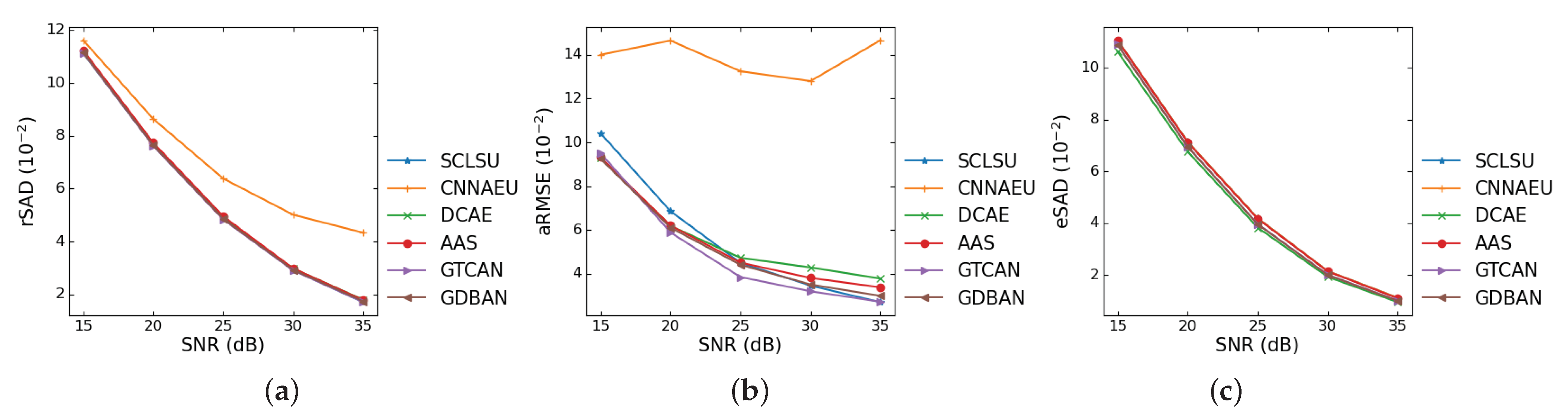
As the compared methods may be sensitive to the signal-to-noise ratio (SNR) of the data, it is indispensable to investigate the robustness to noises. In the following Figure 5, we assess the performances of the compared methods on the synthetic data under different SNRs ranging from 15 dB to 35 dB. The results of rSAD and eSAD of most algorithms are similar and do not show obvious differences. According to Figure 5b, SCLSU does not show good robustness in terms of low SNR cases, but as the SNR increases, its unmixing accuracy improves quickly. DCAE and AAS yield ordinary performances. The performance of the proposed GDBAN is quite stable, and GTCAN achieves the best results in most SNR scenarios, which indicates the superiority of the proposed architecture.
Table 3 lists the running time of each approaches. Since spectral unmixing in this paper is conducted in an unsupervised case, we did not perform any training-validation split of the input data. We used all the pixels for training, and the spatial size of the synthetic data is . Namely, the number of samples is 4900. According to Table 3, SCLSU has the highest efficiency because of the simplicity of the model. DCAE takes the highest time to converge for its deep one-dimensional convolutional encoder network. CNNAEU and AAS spend a moderate amount of time. Due to the application of various network structures, our method does not yield competitive performance in terms of running time.
4.3. Experiments on Real-World Data
In the real-world data experiments, we evaluated the algorithms on three data from three aspects, which are analysis of quantitative unmixing results, abundance analysis from a visual perspective, and hyperparameter sensitivity analysis, respectively. The hyperparameters of facilitating sparsity of GTCAN on Samson, Jasper Ridge and Houston are set as , and , respectively. Accordingly, the of GDBAN is set as , and . The number of training epochs remains 150, and the determination of is analyzed in the following parameter sensitivity analysis.
4.3.1. Experiments on Samson Data
The first experiment is conducted on the Samson data, and the estimated abundance maps are exhibited in Figure 6. It is observed that the abundance maps identified by our proposed methods show high contrast and maintain the best purity. Each map contains regions with clustered high abundance fractions and smooth low fractions, and the estimated distributions are in accordance with natural appearance. It is worth noting that, compared with other methods, GTCAN and GDBAN retain rich edge information for the abundance maps, which is mainly on account of the adaptability of the gating mechanism. For instance, at the junction area of water and soil, even if the abundance changes dramatically on both sides of the boundary, the proposed algorithms can still give precise prediction to the pixels with high abundance fraction. In addition, the abundances estimated by our algorithm show good regional consistency. Taking the abundance maps of water as an example, in land regions, the abundance of water is almost zero without regional errors, which implies the effective utilization of spatial information. The statistical results in Table 4 also verify the above analysis.
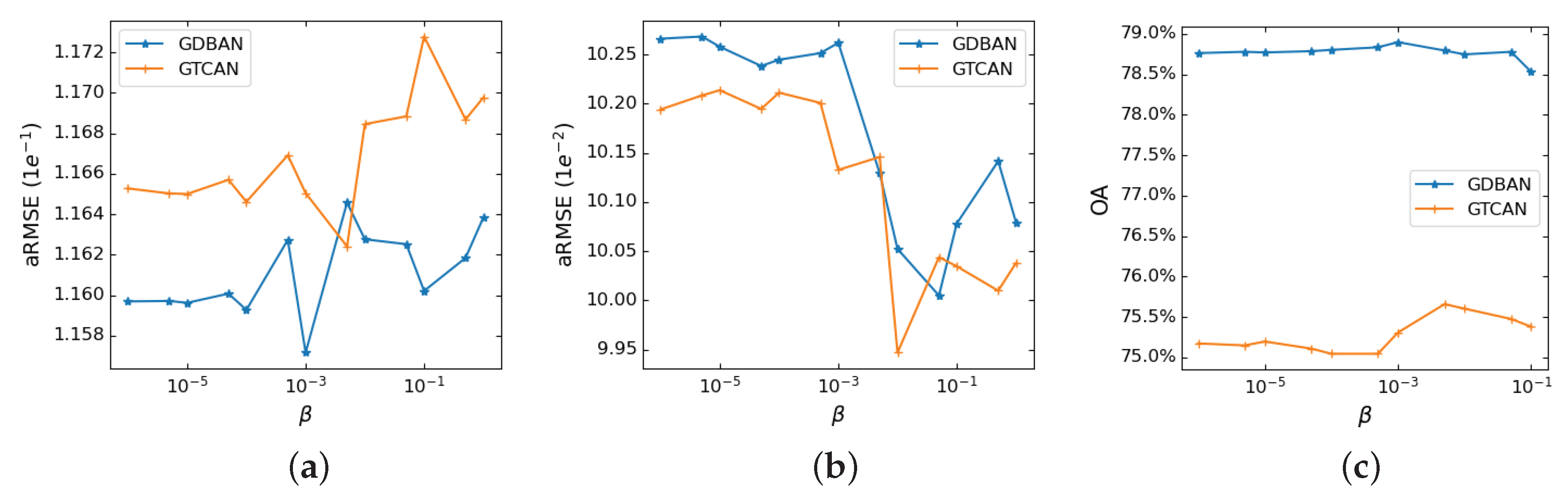
Since the gating mechanism is of great importance to the unmixing performance, we investigate the effects through changing the penalty parameter of gating mechanism. As illustrated in Figure 7, the abundance estimation performances concerning different penalty values on three data are given. A larger value of represents the closure of the gate mechanism. In other words, the spatial information will be used less. Conversely, the smaller means that the spatial information is more preserved. According to Figure 7, the penalty value for obtaining the best abundance estimation is approximately in the range of to . This can be understood that, on the one hand, when the gating regularization becomes stricter, the spatial information will be less helpful to the unmixing. On the other hand, when the gating mechanism is not constrained strictly, it will facilitate the reduction of reconstruction errors while ignoring balancing the effect of spectral information and spatial information on unmixing. Therefore, limiting the value of the mask to an appropriate range is conducive to unmixing performance.
4.3.2. Experiments on Jasper Ridge Data
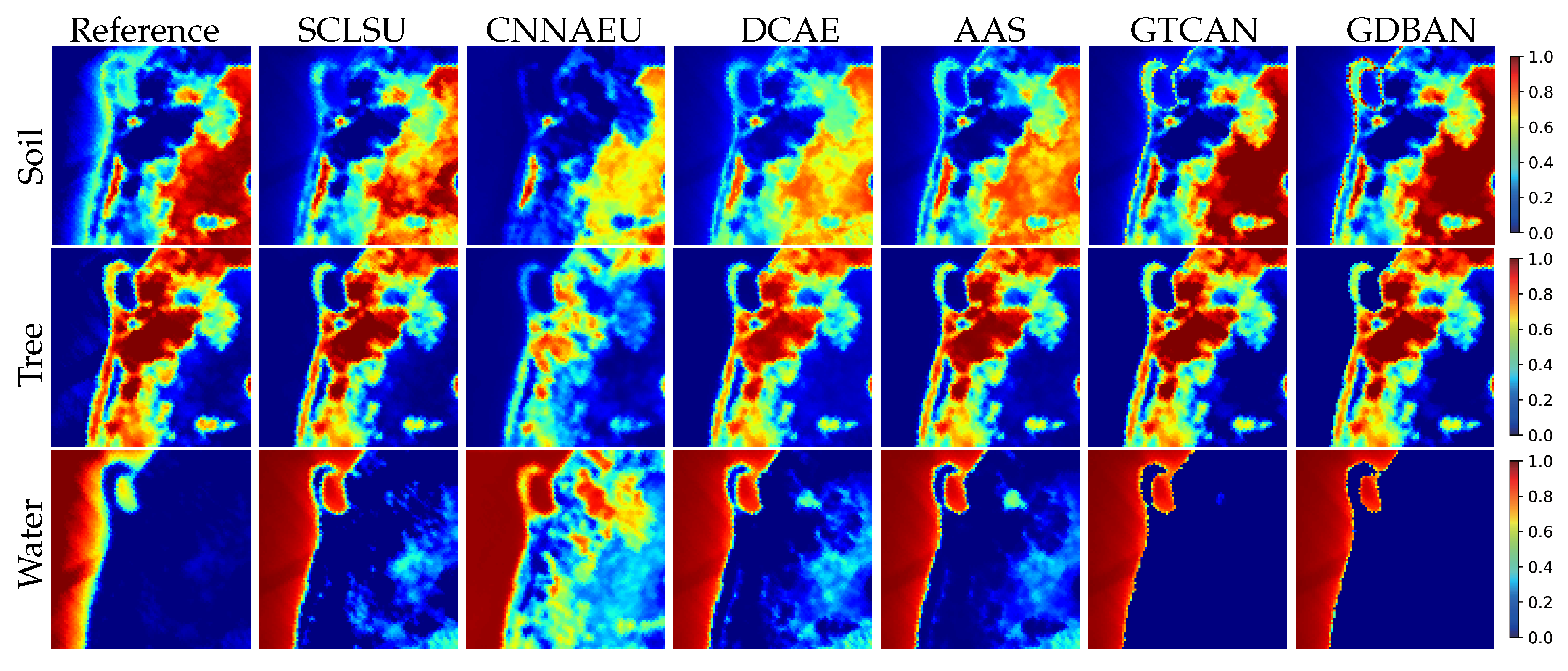
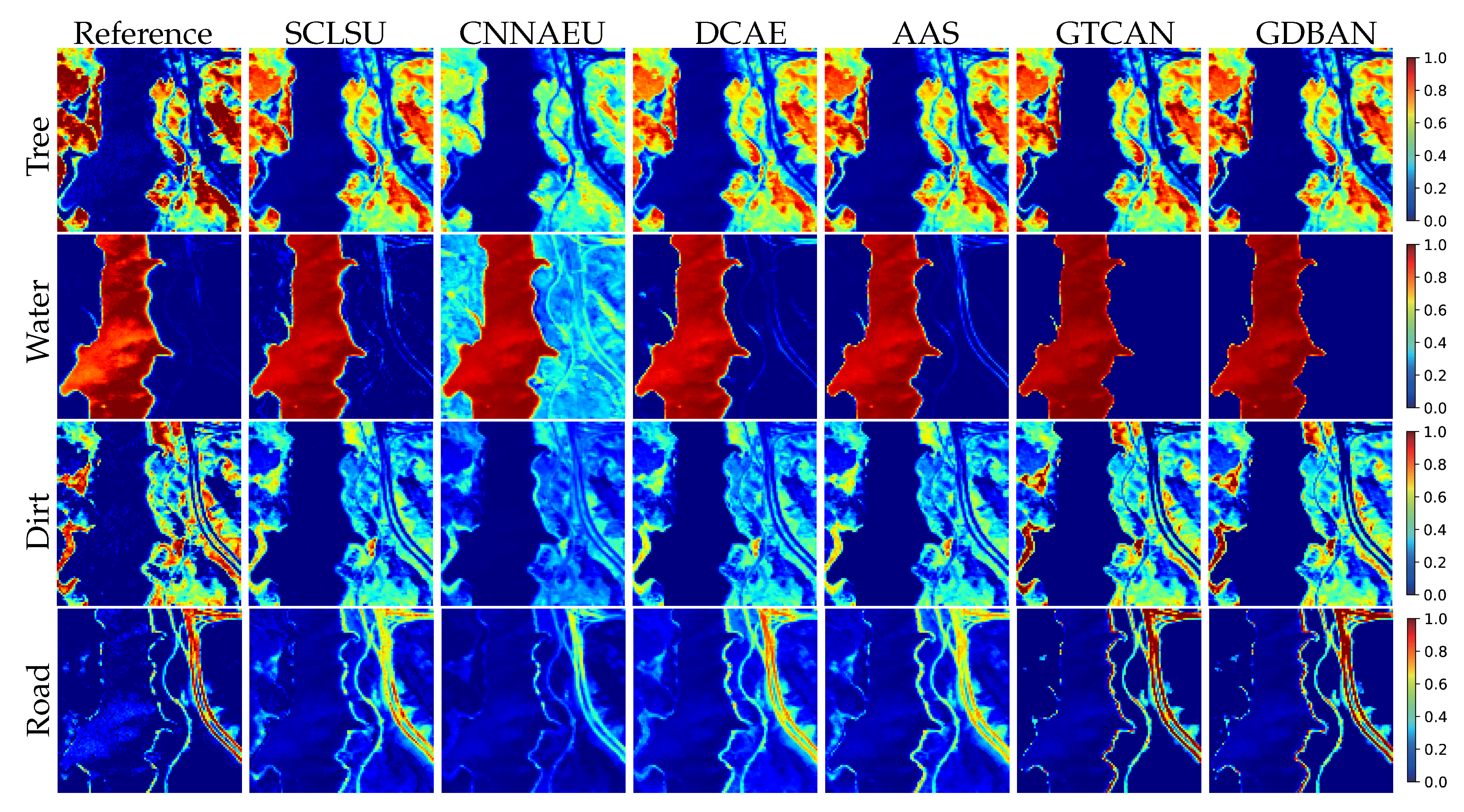
The second real-world scene is Jasper Ridge data, and the visual results are exhibited in Figure 8. We can observe that the abundance maps estimated by the proposed methods maintain the same style as that in the Samson data, which is high contrast and purity and shows the best visual resemblance to the reference maps. For instance, the abundance maps of dirt reflect high contrast because the maps maintain high abundance fractions in clustered areas and clearly indicate the shape of the road, which may result from the moderate application of the sparsity regularization. With regard to the maps of water and road, due to the exploitation of spatial–contextual correlation, the backgrounds (regions of low abundance fraction) present consistency and regional continuity and show the best visual fidelity. The quantitative results are listed in Table 4, where the proposed methods still yield the minimum error concerning each index.
4.3.3. Experiments on Houston Data
Unlike the previous natural scene data, the Houston data is an urban scene data with sharp regional edges and shorter transition areas between substances, which will test the adaptivity of the methods for utilizing spatial information. Due to the lack of reference abundance, we use OA to evaluate the abundance estimation performances of the methods, and the labeled classification-based ground truth is shown in the following Figure 9.
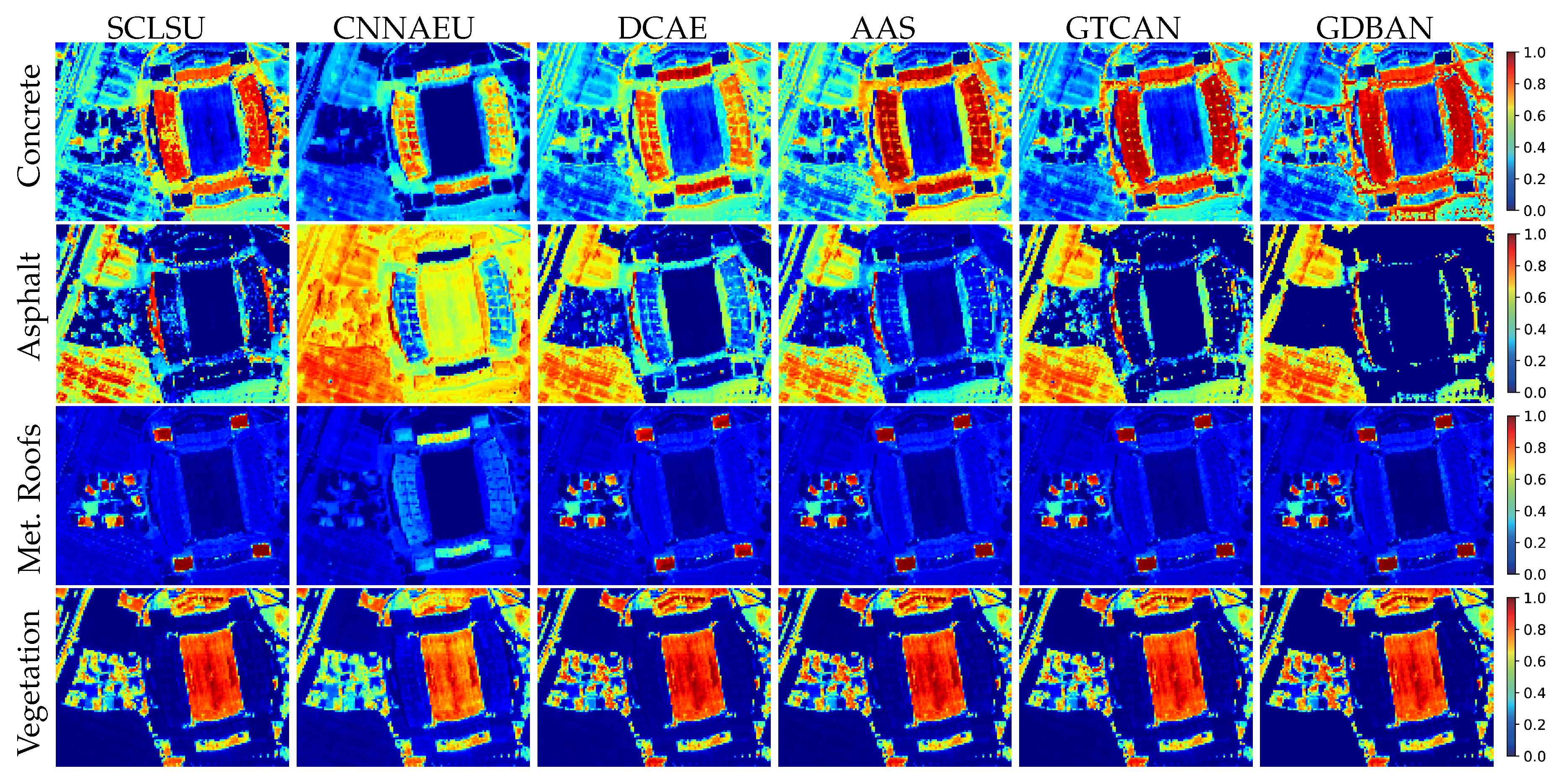
The predicted abundance maps by different algorithms are presented in Figure 10, and the corresponding statistical results are listed in Table 5. We observe that the unmixing performance of GDBAN is outstanding in terms of OA and eSAD. Several reasons may account for this result. First, the classification-based evaluation index, overall accuracy, only judges whether the corresponding endmember of the highest abundance fraction matches the reference material, requiring high-contrast abundance to obtain a satisfying consequence. In addition, the characteristics of urban scene ensure that the distribution of abundance is sparse. Therefore, the sparsity of abundance has a great influence on the unmixing results of this data. However, high sparsity requirements will lead to the increase of reconstruction error, which may cause underfitting and hurt unmixing accuracy. Because of the favorable reconstruction performance and reconstruction stability (low standard derivation) of the proposed algorithm, it can enhance the sparsity of generated abundances without causing degradation of unmixing. Second, it should be noted that GTCAN does not yield similar competitive results as GDBAN. The abundance maps of asphalt will serve as an example. GDBAN suppresses the low abundance fractions to maintain the uniformity of the background, while GTCAN encounters trouble with eliminating the interference caused by alternating roofs and vegetation. The good performance of GDBAN stems from the ability to easily shut down the impact of spatial information because the frequent alternation of the substances provides little useful adjacent information and instead will mislead the solution of unmixing. Compared to GTCAN using a matrix as the mask to filter spatial information, GDBAN only needs to pay attention to one parameter, which is more efficient and convenient. Third, since the spatial–contextual dependence is not satisfied in some regions, the effective extraction of spectral information becomes the key to accurate unmixing. Compared with one-dimensional convolution and three-dimensional convolution, full connection is more efficient in utilizing spectral information for its global receptive field, so GDBAN achieves more acceptable results.
5. Conclusions
The exploitation of spatial information has long been a concern in the field of spectral unmixing. Researchers made plenty of attempts to leverage spatial features to enhance the unmixing accuracy and robustness, which are based on handcrafted designed rules and incorporating adaptive mechanisms. In this paper, aiming at improving the efficient and robust employment of spatial correlation in different scenes, we propose two neural network architectures with sparse and balancing regularizations for spectral–spatial unmixing. The first network, GTCAN, uses a matrix mask to filter the spatial information and adopts three-dimensional convolution to extract spectral and spatial information simultaneously. The second network, GDBAN, leverages the advantages of two-dimensional convolution and full connection in exploiting spatial and spectral information, respectively, and employs concatenated spectral–spatial features in the generation of the spatial attention mask. Furthermore, the sparsity regularization and gate penalty regularization also play their significant roles in contributing to the appropriate implementation of the proposed network. The experiments have validated that, compared with the state-of-the-art unmixing techniques, the proposed methods yield competitive performance in both the synthetic scene and different real-world scenes. In addition, the experiments indicate that there is still room to improve the regularization mechanism for spatial information, which is worth investigating in further research.
Author Contributions
All authors made great contributions to the work. Conceptualization, Z.H.; Methodology, Z.H. and X.L.; Validation, X.L., J.J. and L.Z.; Writing—original draft preparation, Z.H.; Writing—review and editing, X.L. and J.J.; visualization, L.Z.; supervision, Z.H.; funding acquisition, X.L. and J.J. All authors have read and agreed to the published version of the manuscript.
Funding
This research was supported in part by the National Nature Science Foundation of China under Grant 61671408, and in part by the Joint Fund of the Ministry of Education of China under Grant 6141A02022362.
Institutional Review Board Statement
Not applicable.
Informed Consent Statement
Not applicable.
Data Availability Statement
The data used in this study are available at https://www.kaggle.com/ziqhua/hyperspectral-images (accessed on 23 April 2021).
Conflicts of Interest
The authors declare no conflict of interest.
References
- Keshava, N.; Mustard, J.F. Spectral unmixing. IEEE Signal Process. Mag. 2002, 19, 44–57. [Google Scholar] [CrossRef]
- Bhatt, J.S.; Joshi, M.V. Deep Learning in Hyperspectral Unmixing: A Review. In Proceedings of the IGARSS 2020—2020 IEEE International Geoscience and Remote Sensing Symposium, Waikoloa, HI, USA, 26 September–2 October 2020; pp. 2189–2192. [Google Scholar] [CrossRef]
- Heylen, R.; Parente, M.; Gader, P. A Review of Nonlinear Hyperspectral Unmixing Methods. IEEE J. Sel. Top. Appl. Earth Obs. Remote Sens. 2014, 7, 1844–1868. [Google Scholar] [CrossRef]
- Shi, C.; Wang, L. Incorporating spatial information in spectral unmixing: A review. Remote Sens. Environ. 2014, 149, 70–87. [Google Scholar] [CrossRef]
- Borsoi, R.A.; Imbiriba, T.; Bermudez, J.C.M.; Richard, C.; Chanussot, J.; Drumetz, L.; Tourneret, J.Y.; Zare, A.; Jutten, C. Spectral Variability in Hyperspectral Data Unmixing: A Comprehensive Review. arXiv 2020, arXiv:2001.07307. [Google Scholar]
- Ibarrola-Ulzurrun, E.; Drumetz, L.; Marcello, J.; Gonzalo-Martín, C.; Chanussot, J. Hyperspectral Classification Through Unmixing Abundance Maps Addressing Spectral Variability. IEEE Trans. Geosci. Remote Sens. 2019, 57, 4775–4788. [Google Scholar] [CrossRef]
- Guo, A.J.; Zhu, F. Improving deep hyperspectral image classification performance with spectral unmixing. Signal Process. 2021, 183, 107949. [Google Scholar] [CrossRef]
- Zou, C.; Huang, X. Hyperspectral image super-resolution combining with deep learning and spectral unmixing. Signal Process. Image Commun. 2020, 84, 115833. [Google Scholar] [CrossRef]
- Li, J.; Peng, Y.; Jiang, T.; Zhang, L.; Long, J. Hyperspectral Image Super-Resolution Based on Spatial Group Sparsity Regularization Unmixing. Appl. Sci. 2020, 10. [Google Scholar] [CrossRef]
- Hasan, A.F.; Laurent, F.; Messner, F.; Bourgoin, C.; Blanc, L. Cumulative disturbances to assess forest degradation using spectral unmixing in the northeastern Amazon. Appl. Veg. Sci. 2019, 22, 394–408. [Google Scholar] [CrossRef]
- Li, H.; Zhang, L. A Hybrid Automatic Endmember Extraction Algorithm Based on a Local Window. IEEE Trans. Geosci. Remote Sens. 2011, 49, 4223–4238. [Google Scholar] [CrossRef]
- Deng, C.; Wu, C. A spatially adaptive spectral mixture analysis for mapping subpixel urban impervious surface distribution. Remote Sens. Environ. 2013, 133, 62–70. [Google Scholar] [CrossRef]
- Jia, S.; Qian, Y. Constrained Nonnegative Matrix Factorization for Hyperspectral Unmixing. IEEE Trans. Geosci. Remote Sens. 2009, 47, 161–173. [Google Scholar] [CrossRef]
- Castrodad, A.; Xing, Z.; Greer, J.B.; Bosch, E.; Carin, L.; Sapiro, G. Learning Discriminative Sparse Representations for Modeling, Source Separation, and Mapping of Hyperspectral Imagery. IEEE Trans. Geosci. Remote Sens. 2011, 49, 4263–4281. [Google Scholar] [CrossRef]
- Iordache, M.; Bioucas-Dias, J.M.; Plaza, A. Total Variation Spatial Regularization for Sparse Hyperspectral Unmixing. IEEE Trans. Geosci. Remote Sens. 2012, 50, 4484–4502. [Google Scholar] [CrossRef] [Green Version]
- Liu, J.; Zhang, J.; Gao, Y.; Zhang, C.; Li, Z. Enhancing Spectral Unmixing by Local Neighborhood Weights. IEEE J. Sel. Top. Appl. Earth Obs. Remote Sens. 2012, 5, 1545–1552. [Google Scholar] [CrossRef]
- He, W.; Zhang, H.; Zhang, L. Total Variation Regularized Reweighted Sparse Nonnegative Matrix Factorization for Hyperspectral Unmixing. IEEE Trans. Geosci. Remote Sens. 2017, 55, 3909–3921. [Google Scholar] [CrossRef]
- Borsoi, R.A.; Imbiriba, T.; Bermudez, J.C.M.; Richard, C. A Fast Multiscale Spatial Regularization for Sparse Hyperspectral Unmixing. IEEE Geosci. Remote Sens. Lett. 2019, 16, 598–602. [Google Scholar] [CrossRef] [Green Version]
- Yuan, Y.; Zhang, Z.; Wang, Q. Improved Collaborative Non-Negative Matrix Factorization and Total Variation for Hyperspectral Unmixing. IEEE J. Sel. Top. Appl. Earth Obs. Remote Sens. 2020, 13, 998–1010. [Google Scholar] [CrossRef]
- Li, H.; Feng, R.; Wang, L.; Zhong, Y.; Zhang, L. Superpixel-Based Reweighted Low-Rank and Total Variation Sparse Unmixing for Hyperspectral Remote Sensing Imagery. IEEE Trans. Geosci. Remote Sens. 2021, 59, 629–647. [Google Scholar] [CrossRef]
- Wang, J.J.; Huang, T.Z.; Huang, J.; Deng, L.J. A two-step iterative algorithm for sparse hyperspectral unmixing via total variation. Appl. Math. Comput. 2021, 401, 126059. [Google Scholar] [CrossRef]
- Hua, Z.; Li, X.; Qiu, Q.; Zhao, L. Autoencoder Network for Hyperspectral Unmixing with Adaptive Abundance Smoothing. IEEE Geosci. Remote Sens. Lett. 2020, 1–5. [Google Scholar] [CrossRef]
- Su, Y.; Marinoni, A.; Li, J.; Plaza, J.; Gamba, P. Stacked Nonnegative Sparse Autoencoders for Robust Hyperspectral Unmixing. IEEE Geosci. Remote Sens. Lett. 2018, 15, 1427–1431. [Google Scholar] [CrossRef]
- Ozkan, S.; Kaya, B.; Akar, G.B. EndNet: Sparse AutoEncoder Network for Endmember Extraction and Hyperspectral Unmixing. IEEE Trans. Geosci. Remote Sens. 2019, 57, 482–496. [Google Scholar] [CrossRef] [Green Version]
- Qu, Y.; Qi, H. uDAS: An Untied Denoising Autoencoder With Sparsity for Spectral Unmixing. IEEE Trans. Geosci. Remote Sens. 2019, 57, 1698–1712. [Google Scholar] [CrossRef]
- Zhao, Z.; Hu, D.; Wang, H.; Yu, X. Minimum distance constrained sparse autoencoder network for hyperspectral unmixing. J. Appl. Remote Sens. 2020, 14, 1–15. [Google Scholar] [CrossRef]
- Dou, Z.; Gao, K.; Zhang, X.; Wang, H.; Wang, J. Hyperspectral Unmixing Using Orthogonal Sparse Prior-Based Autoencoder With Hyper-Laplacian Loss and Data-Driven Outlier Detection. IEEE Trans. Geosci. Remote Sens 2020, 58, 6550–6564. [Google Scholar] [CrossRef]
- Elkholy, M.M.; Mostafa, M.; Ebied, H.M.; Tolba, M.F. Hyperspectral unmixing using deep convolutional autoencoder. Int. J. Remote Sens. 2020, 41, 4799–4819. [Google Scholar] [CrossRef]
- Palsson, B.; Ulfarsson, M.O.; Sveinsson, J.R. Convolutional Autoencoder for Spectral–Spatial Hyperspectral Unmixing. IEEE Trans. Geosci. Remote Sens. 2021, 59, 535–549. [Google Scholar] [CrossRef]
- Hochreiter, S.; Schmidhuber, J. Long short-term memory. Neural Comput. 1997, 9, 1735–1780. [Google Scholar] [CrossRef]
- Cho, K.; van Merrienboer, B.; Gülçehre, Ç.; Bougares, F.; Schwenk, H.; Bengio, Y. Learning Phrase Representations using RNN Encoder-Decoder for Statistical Machine Translation. arXiv 2014, arXiv:1406.1078. [Google Scholar]
- Hu, J.; Shen, L.; Sun, G. Squeeze-and-Excitation Networks. In Proceedings of the IEEE Conference on Computer Vision and Pattern Recognition (CVPR), Salt Lake City, UT, USA, 18–23 June 2018. [Google Scholar]
- Fu, J.; Liu, J.; Tian, H.; Li, Y.; Bao, Y.; Fang, Z.; Lu, H. Dual Attention Network for Scene Segmentation. In Proceedings of the IEEE/CVF Conference on Computer Vision and Pattern Recognition (CVPR), Long Beach, CA, USA, 16–20 June 2019. [Google Scholar]
- Xu, Z.; Zhang, H.; Wang, Y.; Chang, X.; Liang, Y. L1/2 regularization. Sci. China Inf. Sci. 2010, 53, 1159–1169. [Google Scholar] [CrossRef] [Green Version]
- Qian, Y.; Jia, S.; Zhou, J.; Robles-Kelly, A. Hyperspectral Unmixing via L1/2 Sparsity-Constrained Nonnegative Matrix Factorization. IEEE Trans. Geosci. Remote Sens. 2011, 49, 4282–4297. [Google Scholar] [CrossRef] [Green Version]
- Hong, D.; Yokoya, N.; Chanussot, J.; Zhu, X.X. An Augmented Linear Mixing Model to Address Spectral Variability for Hyperspectral Unmixing. IEEE Trans. Image Process. 2019, 28, 1923–1938. [Google Scholar] [CrossRef] [PubMed] [Green Version]
- Clark, R.N.; Swayze, G.A.; Wise, R.A.; Livo, K.E.; Hoefen, T.M.; Kokaly, R.F.; Sutley, S.J. USGS Digital Spectral Library splib06a; Technical Report; US Geological Survey: Reston, VA, USA, 2007. [Google Scholar]
- Grupo de Inteligencia Computacional, Universidad del País Vasco/Euskal Herriko Unibertsitatea. Hyperspectral Imagery Synthesis Toolbox; Universidad del País Vasco/Euskal Herriko Unibertsitatea (UPV/EHU): Leioa, Spain, 2021. [Google Scholar]
- Zhu, F.; Wang, Y.; Fan, B.; Xiang, S.; Meng, G.; Pan, C. Spectral Unmixing via Data-Guided Sparsity. IEEE Trans. Image Process. 2014, 23, 5412–5427. [Google Scholar] [CrossRef] [PubMed] [Green Version]
- Nascimento, J.M.P.; Dias, J.M.B. Vertex component analysis: A fast algorithm to unmix hyperspectral data. IEEE Trans. Geosci. Remote Sens. 2005, 43, 898–910. [Google Scholar] [CrossRef] [Green Version]
Figure 1.
Architecture of gated three-dimensional convolutional autoencoder network.
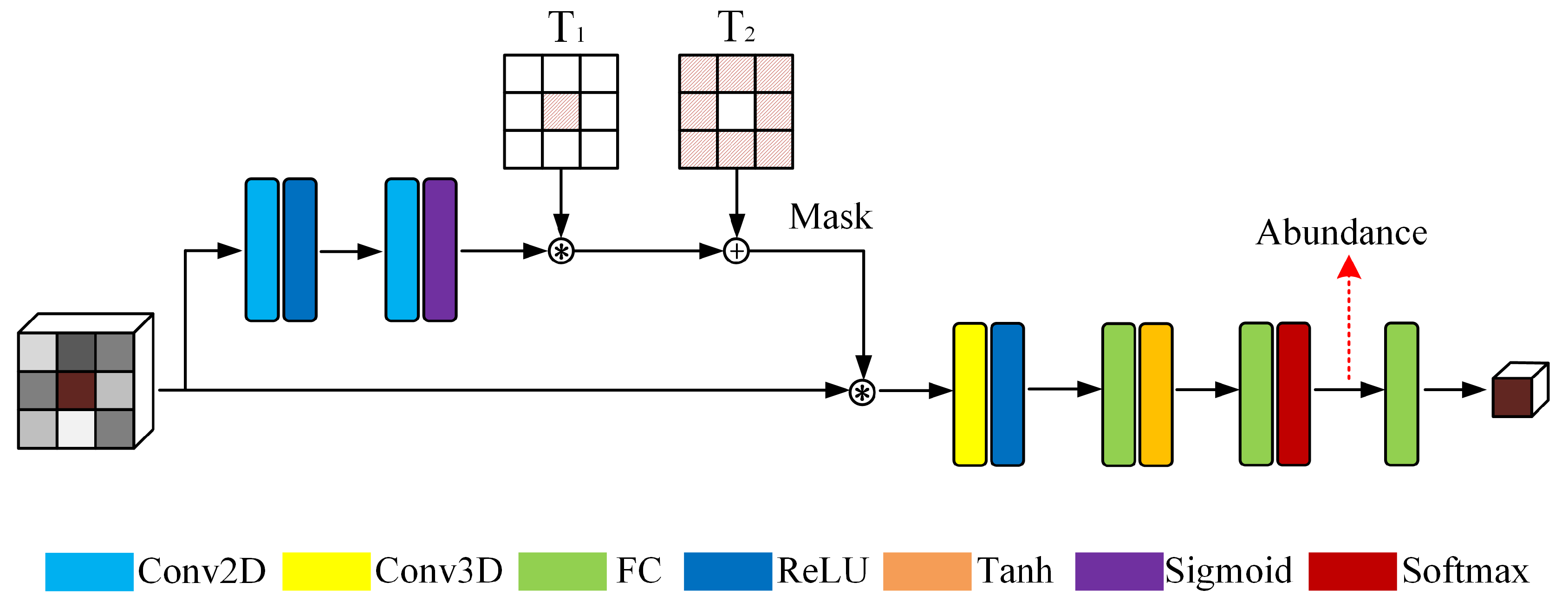
Figure 2.
Architecture of gated dual branch autoencoder network.
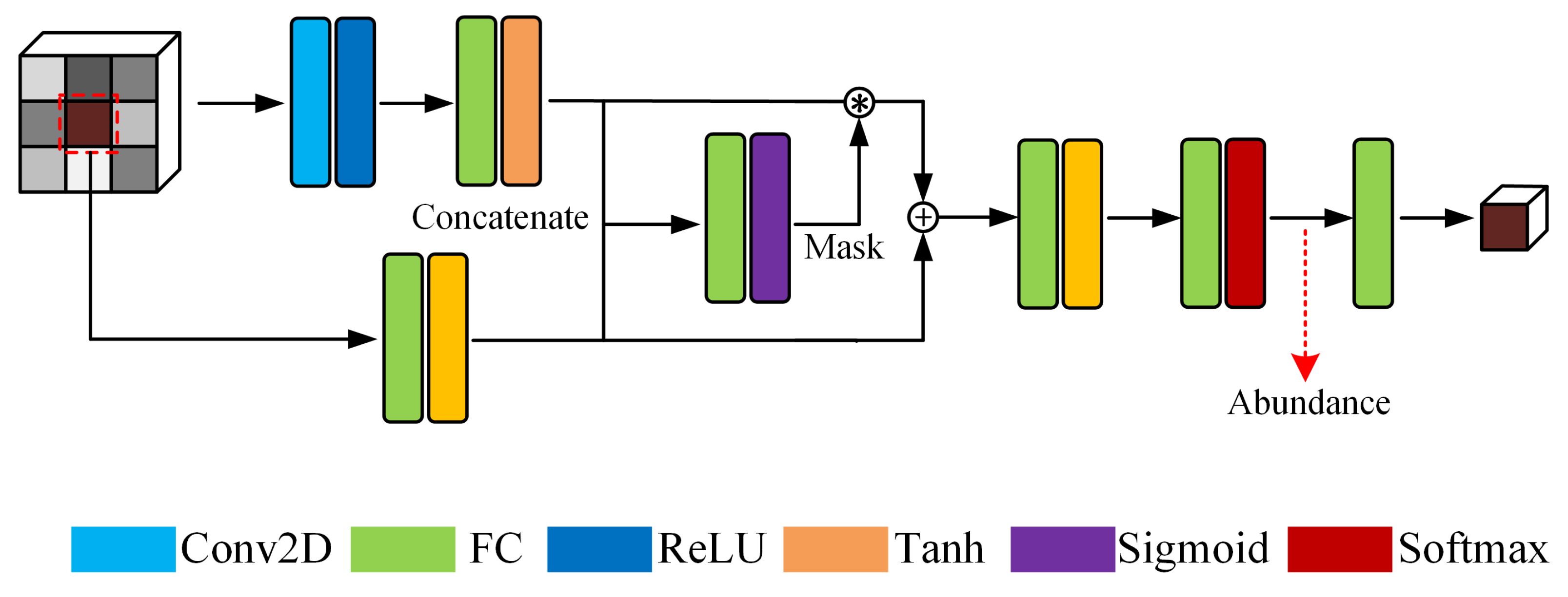
Figure 3.
A pseudo color image of synthetic data and endmembers. (a) Pseudo color image. (b) Endmember spectra.
Figure 3.
A pseudo color image of synthetic data and endmembers. (a) Pseudo color image. (b) Endmember spectra.
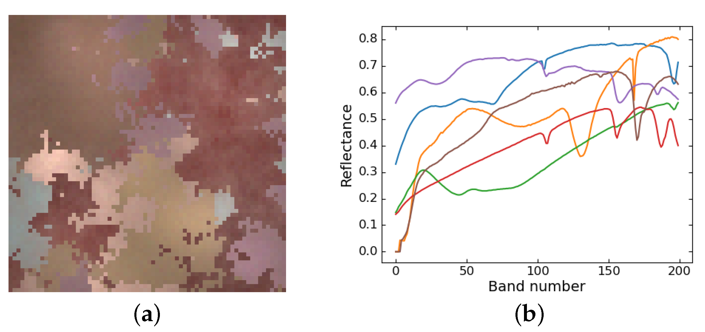
Figure 4.
Absolute error maps of the estimated abundances on synthetic data by different methods.
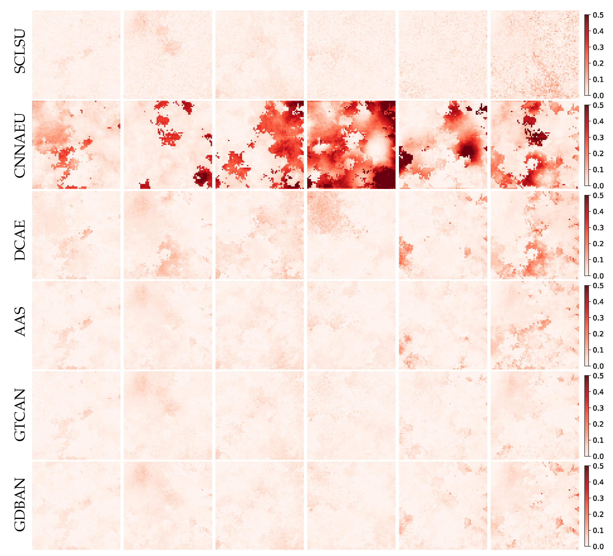
Figure 5.
Robustness analysis with the different SNRs. (a) rSAD. (b) aRMSE. (c) eSAD.

Figure 6.
Reference and estimated abundance maps on Samson data by different methods.

Figure 7.
Parameter sensitivity analysis of gating mechanism. (a) Samson scene. (b) Jasper Ridge scene. (c) Houston scene.
Figure 7.
Parameter sensitivity analysis of gating mechanism. (a) Samson scene. (b) Jasper Ridge scene. (c) Houston scene.

Figure 8.
Reference and estimated abundance maps on Jasper Ridge data by different methods.

Figure 9.
Ground truth of Houston data.
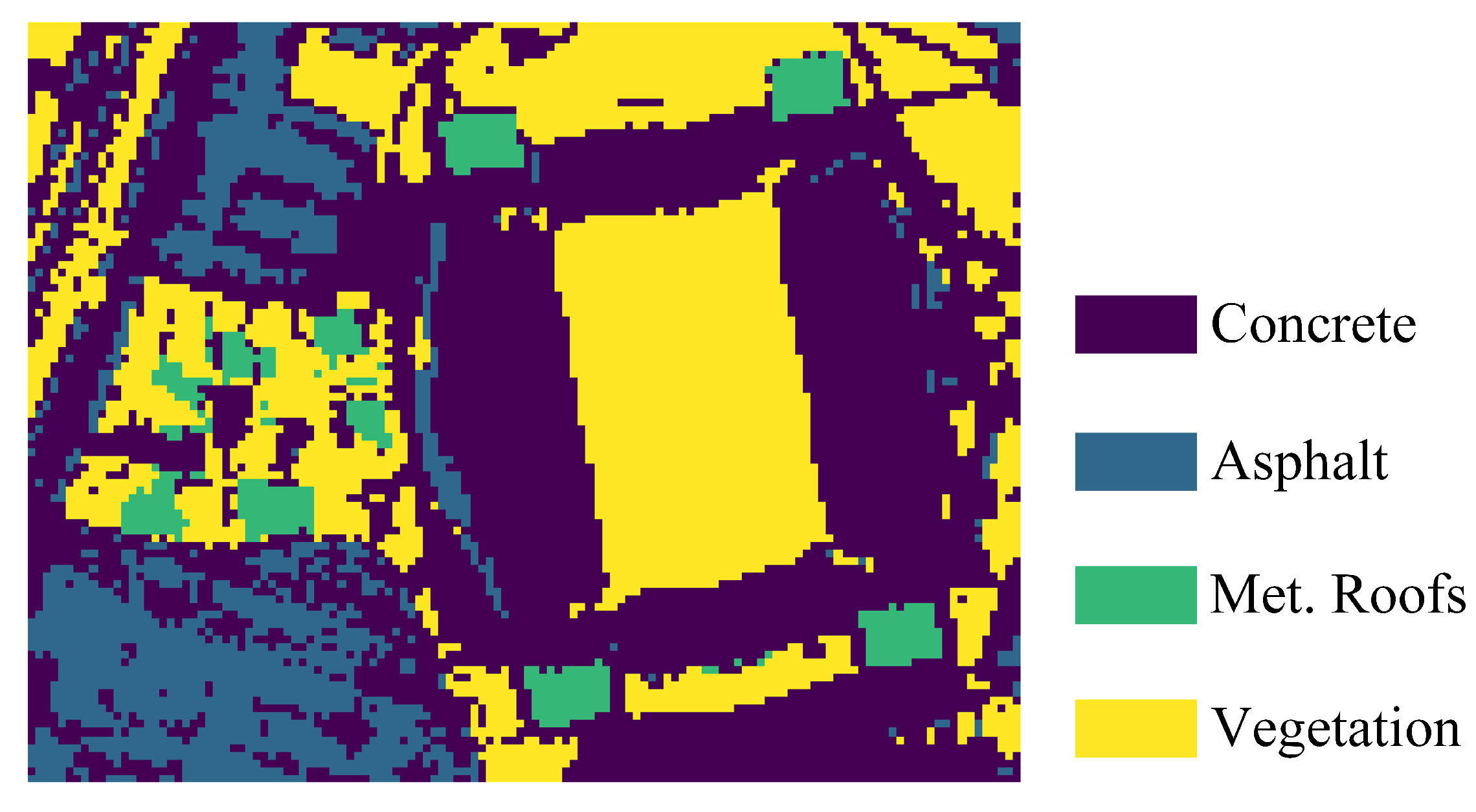
Figure 10.
Estimated abundance maps on Houston data by different methods.

Table 1.
Network configuration of the proposed architectures. The number of input channel is omitted.
Table 1.
Network configuration of the proposed architectures. The number of input channel is omitted.
| GTDAN | GDBAN |
|---|---|
| Gated Net | First Branch |
| Conv2D, size = , channel = 16, padding = 1 | Conv2D, size = , channel = 128 |
| Conv2D, size = , channel = 1, padding = 1 | FC, length = 64 |
| AE Net | Second Branch |
| Conv3D, size = , channel = 16 | FC, length = 64 |
| FC, length = 64 | Gated Net |
| FC, length = P | FC, length = 1 |
| FC, length = L, bias = false | The Rest |
| FC, length = 32 | |
| FC, length = P | |
| FC, length = L, bias = false |
Table 2.
Quantitative results on synthetic data (SNR = 30 dB). The optimal results are bolded.
| Methods | rSAD | aRMSE | eSAD |
|---|---|---|---|
| SCLSU | 2.90 ± 0.12 | 3.17 ± 0.25 | 1.89 ± 0.23 |
| CNNAEU | 5.01 ± 0.67 | 12.79 ± 4.66 | 1.88 ± 0.23 |
| DCAE | 2.95 ± 0.12 | 3.88 ± 0.40 | 1.63 ± 0.23 |
| AAS | 2.96 ± 0.12 | 3.55 ± 0.25 | 1.87 ± 0.23 |
| GTCAN | 2.88 ± 0.12 | 2.85 ± 0.21 | 1.66 ± 0.24 |
| GDBAN | 2.90 ± 0.12 | 3.18 ± 0.21 | 1.65 ± 0.23 |
Table 3.
Running time comparison.
| Methods | SCLSU | CNNAEU | DCAE | AAS | GTCAN | GDBAN |
|---|---|---|---|---|---|---|
| Time (s) | 1 | 34 | 99 | 38 | 86 | 72 |
Table 4.
Quantitative results on Samson and Jasper Ridge data. The optimal results are bolded.
| Data | Methods | rSAD | aRMSE | eSAD |
|---|---|---|---|---|
| Samson | SCLSU | 5.22 ± 0.25 | 13.27 ± 2.34 | 6.61 ± 0.26 |
| CNNAEU | 10.35 ± 1.02 | 24.13 ± 0.65 | 6.59 ± 0.26 | |
| DCAE | 3.76 ± 0.08 | 14.94 ± 1.68 | 6.57 ± 1.40 | |
| AAS | 5.30 ± 0.25 | 13.11 ± 2.35 | 6.54 ± 0.29 | |
| GTCAN | 3.45 ± 0.03 | 10.94 ± 1.35 | 6.56 ± 1.04 | |
| GDBAN | 3.45 ± 0.04 | 11.04 ± 1.41 | 6.51 ± 1.08 | |
| Jasper Ridge | SCLSU | 12.55 ± 5.82 | 18.41 ± 3.01 | 24.43 ± 5.73 |
| CNNAEU | 16.19 ± 6.21 | 17.90 ± 1.80 | 24.43 ± 5.73 | |
| DCAE | 8.92 ± 3.42 | 17.08 ± 3.39 | 22.76 ± 4.95 | |
| AAS | 12.49 ± 5.91 | 17.68 ± 3.36 | 24.18 ± 5.72 | |
| GTCAN | 6.60 ± 0.46 | 16.24 ± 3.39 | 21.27 ± 5.08 | |
| GDBAN | 6.51 ± 0.45 | 16.23 ± 3.24 | 23.20 ± 7.25 |
Table 5.
Quantitative results on Houston data. The optimal results are bolded.
| Methods | rSAD | OA | eSAD |
|---|---|---|---|
| SCLSU | 4.04 ± 0.84 | 71.33 ± 13.85 | 7.59 ± 0.68 |
| CNNAEU | 11.56 ± 1.81 | 59.23 ± 6.71 | 7.55 ± 0.68 |
| DCAE | 3.08 ± 0.65 | 73.51 ± 12.70 | 7.35 ± 0.71 |
| AAS | 4.10 ± 0.74 | 74.72 ± 15.59 | 7.55 ± 0.67 |
| GTCAN | 2.48 ± 0.43 | 75.71 ± 16.26 | 7.39 ± 0.77 |
| GDBAN | 2.76 ± 0.33 | 78.62 ± 16.41 | 6.06 ± 1.23 |
Publisher’s Note: MDPI stays neutral with regard to jurisdictional claims in published maps and institutional affiliations. |
© 2021 by the authors. Licensee MDPI, Basel, Switzerland. This article is an open access article distributed under the terms and conditions of the Creative Commons Attribution (CC BY) license (https://creativecommons.org/licenses/by/4.0/).
Share and Cite
MDPI and ACS Style
Hua, Z.; Li, X.; Jiang, J.; Zhao, L. Gated Autoencoder Network for Spectral–Spatial Hyperspectral Unmixing. Remote Sens. 2021, 13, 3147. https://0-doi-org.brum.beds.ac.uk/10.3390/rs13163147
AMA Style
Hua Z, Li X, Jiang J, Zhao L. Gated Autoencoder Network for Spectral–Spatial Hyperspectral Unmixing. Remote Sensing. 2021; 13(16):3147. https://0-doi-org.brum.beds.ac.uk/10.3390/rs13163147
Chicago/Turabian StyleHua, Ziqiang, Xiaorun Li, Jianfeng Jiang, and Liaoying Zhao. 2021. "Gated Autoencoder Network for Spectral–Spatial Hyperspectral Unmixing" Remote Sensing 13, no. 16: 3147. https://0-doi-org.brum.beds.ac.uk/10.3390/rs13163147
Note that from the first issue of 2016, this journal uses article numbers instead of page numbers. See further details here.