Automated Rain Detection by Dual-Polarization Sentinel-1 Data

Abstract

Rain Signatures on C-band Synthetic Aperture Radar (SAR) images acquired over ocean are common and can dominate the backscattered signal from the ocean surface. In many cases, the inability to decipher between ocean and rain signatures can disturb the analysis of SAR scenes for maritime applications. This study relies on Sentinel-1 SAR acquisitions in the Interferometric Wide swath mode and high-resolution measurements from ground-based weather radar to document the rain impact on the radar backscattered signal in both co- and cross-polarization channels. The dark and bright rain signatures are found in connection with the timeliness of the rain cells. In particular, the bright patches are demonstrated by the hydrometeors (graupels, hails) in the melting layer. In general, the radar backscatter under rain increases with rain rate for a given sea state and decreases when the sea state strengthens. The rain also has a stronger impact on the radar signal in both polarizations when the incidence angle increases. The complementary sensitivity of the SAR signal of rain in both channels is then used to derive a filter to locate the areas in SAR scenes where the signal is not dominated by rain. The filter optimized to match the rain observed by the ground-based weather radar is more efficient when both polarization channels are considered. Case studies are presented to discuss the advantages and limitations of such a filtering approach.

1. Introduction

Space-borne C-band Synthetic Aperture Radar (SAR) has now become an operational component of the existing Earth Observation (EO) network and is commonly used for investigating air–sea interactions from space. In particular, Copernicus, the European program for EO, includes a constellation of two C-band SAR, Sentinel-1A (2014) and Sentinel-1B (2016), and the Canadian Space Agency also recently launched the Radarsat Constellation Mission (2019), a new constellation of 3 satellites with a C-band SAR payload. These two operational programs have also defined dedicated acquisition strategies for SAR-based maritime applications. Copernicus level-2 ocean products encompasses waves (OSW), wind (OWI) and radial surface velocities (RVL) measurements. However, many other ocean and atmospheric geophysical phenomena such as oceanic front, convective cells, modulation of the stress in the marine atmospheric boundary layer or rain [1,2] also affect the signal. Although routinely available since the Radarsat-2 mission, the use of dual-polarization measurements for ocean processes analysis and level-2 ocean product definition is still emerging. Up to now, most of the work has been devoted to the analysis of oceanic fronts [3,4], surface currents [5], hurricanes wind forcing [6,7,8], slicks [9], or sea ice [10,11,12,13].

Studies on rain signatures in SAR imagery is still limited although such signatures can lead to significant errors during wind field or ocean waves spectrum inversion as they impact both the averaged signal and its wave-induced modulation when performing a spectral analysis. Fu and Holt [1] first documented the rain signatures for L-band and studies for X-band and C-band are then devoted [14,15,16,17]. Melsheimer et al. [14] compared the rain signatures simultaneously acquired at L-, X-, C-bands based on SIR-C/X-SAR data. For L-band, negative impacts of rain on the NRCS are observed usually attributed to the surface contribution through wave damping since the atmospheric effects are negligible with no attenuation for the large radar wavelengths. For X-band, surface scattering from ring wave and splash products together with the volume scattering in the atmosphere are expected to increase NRCS. The reduction behind the enhancement is interpreted by the attenuation in the atmosphere along the incident path. C-band lies between X- and L-band, and thus the impact of surface scattering on the radar signal of rain can give rise to both positive and negative contributions [18]. Additionally, the volume scattering and attenuation in the atmosphere cannot always be ignored especially under heavy precipitation [17,19,20]. Thus, the rain signatures at C-band are a combination of different contributions from the atmosphere (volume scattering and attenuation of hydrometeors) and sea surface roughness enhancement/decrease (surface scattering). The multiple contributions lead to the concurrent irregular bright and/or dark areas observed at C-band.

In addition, the rain signature is also sensitive to incidence angle and polarization. Braun and Gade [18] investigated the signatures with multi-frequency and multi-polarization scatterometers, including Doppler, has shown that the contribution due to scattering at stalks increases at HH polarization when the incidence angle increases, whereas the ring-wave impact decreases. Apart from the relative contribution from the surface scattering mechanisms, the attenuation and the volume scattering along the incident path in the atmosphere varies with incidence angle and thus the radar cross-section are incidence angle dependent. In the case of cross-polarization, Melsheimer et al. [14] showed that the signal at cross-polarization is more pronounced with respect to co-polarization. Alpers et al. [17] show several cases revealing that the signal-to-noise ratio is often too low for investigating the impact of rain effects such as the downdraft or the waves damping on the SAR images. However, areas associated with bright patches on the VV images are also visible as bright area on VH polarization channel and probably not due to Bragg scattering from ring waves but to enhanced roughness from splash products [17] or from scattering of hydrometeors in the melting layer [21].

These continuous studies have revealed that the complicated mechanisms of rain signatures at C-band SAR images. However, given the multiple factors intertwined on radar backscatter, it is quite challenging to figure out how strong the sensitivity of received radar backscatter to the rain rate. Lin et al. [22] showed that the statistics of VV-pol NRCS significantly increases even under light rain by collocating ASCAT NRCS data with TRMM/TMI rain data and wind speed from an atmospheric model. This impact decreases with increasing wind speed. In particular, for wind speeds larger than 15 m/s and for rain rates considered in this study, the effect is found to be negligible. However, the 25-km resolution of ASCAT NRCS measurements does not allow the capture of the full complexity observed in the SAR data at high resolution [17,23]. Recently, in a case study, Liu et al. [24] compared an ENVISAT/ASAR image with weather radar data from a station in Taiwan. They found that the NRCS increases with base reflectivity up to 45 dBZ (∼rain rate 24 mm/h) and then decreases gradually, showing a different trend from what is expected from scatterometer data. This case study, as well as the detailed study from Melsheimer et al. [23], point to the necessity of having collocated measurements with high-resolution ground-based weather radars and SARs to further investigate the relationship between NRCS and rain intensity. Apart from that, the radar backscatter under cross-polarization is not quantitatively compared to co-polarization.

In this study, we take advantage of the Sentinel-1 that provides a large amount of data close to the coast in co- and cross-polarization collocated with operational weather radar stations. Based on this dataset, we aim to document the different behaviors of high-resolution co-/cross-pol NRCS in response to intensifying rain rate and wind speed. This high-resolution investigation would help to understand the wind-rain interaction and provide a reference to rain signature recognition. Moreover, according to the collocated dataset, we propose a dual-polarization filter to detect the rain signatures. The systematic detection of heterogeneity objects in SAR images not associated with meso-scale winds has been investigated by Koch [25] only for single-polarization. Given the cross-pol contribution, the dual-polarization filter significantly improves the detection accuracy of rain signatures.

The paper is organized as follows: In Section 2 the dataset is described. Section 3 characterizes the rain impact on SAR image with respect to rain rate, background wind speed as a function of polarization, and incidence angle. In Section 4, we propose a method to detect rain signatures based on the dual-polarization acquisitions. Section 5 presents our conclusions and perspectives.

2. Dataset

To investigate the impact of rainfall on C-band SAR backscattering and develop an automated rain area detection for SAR images, we need both SAR and rain rate measurements. To this aim, we systematically collocate Sentinel-1 data and weather radar data from the National Oceanic Atmospheric Administration (NOAA) and the Japanese Meteorological Agency (JMA). This section describes these data and the collocation method.

2.1. Sentinel-1

Sentinel-1 is a satellite constellation carrying C-band SARs, with Sentinel-1A (S-1A) and Sentinel-1B (S-1B) launched in April 2014 and April 2016, respectively. They operate with four exclusive modes, Interferometric Wide Swath (IW) mode, Extra Wide Swath (EW) mode, StripMap (SM) mode, and Wave (WV) mode. Among these modes, IW is the main acquisition mode over coastal and land areas. The spatial resolution of IW is 5 m by 20 m and its incidence angles range from 29${}^{\circ }$ to 46${}^{\circ }$ with a swath width of 250 km. IW can operate at dual (VV + VH/HH + HV) or single (VV/HH) polarization. In this study, we focus on S-1 IW acquisitions (VV + VH) from March 2015 to November 2020. This is the default mode over coastal areas. The leakage from VV to VH channels is considered to be negligible as described in Longépé et al. [26].

2.2. Weather Radar

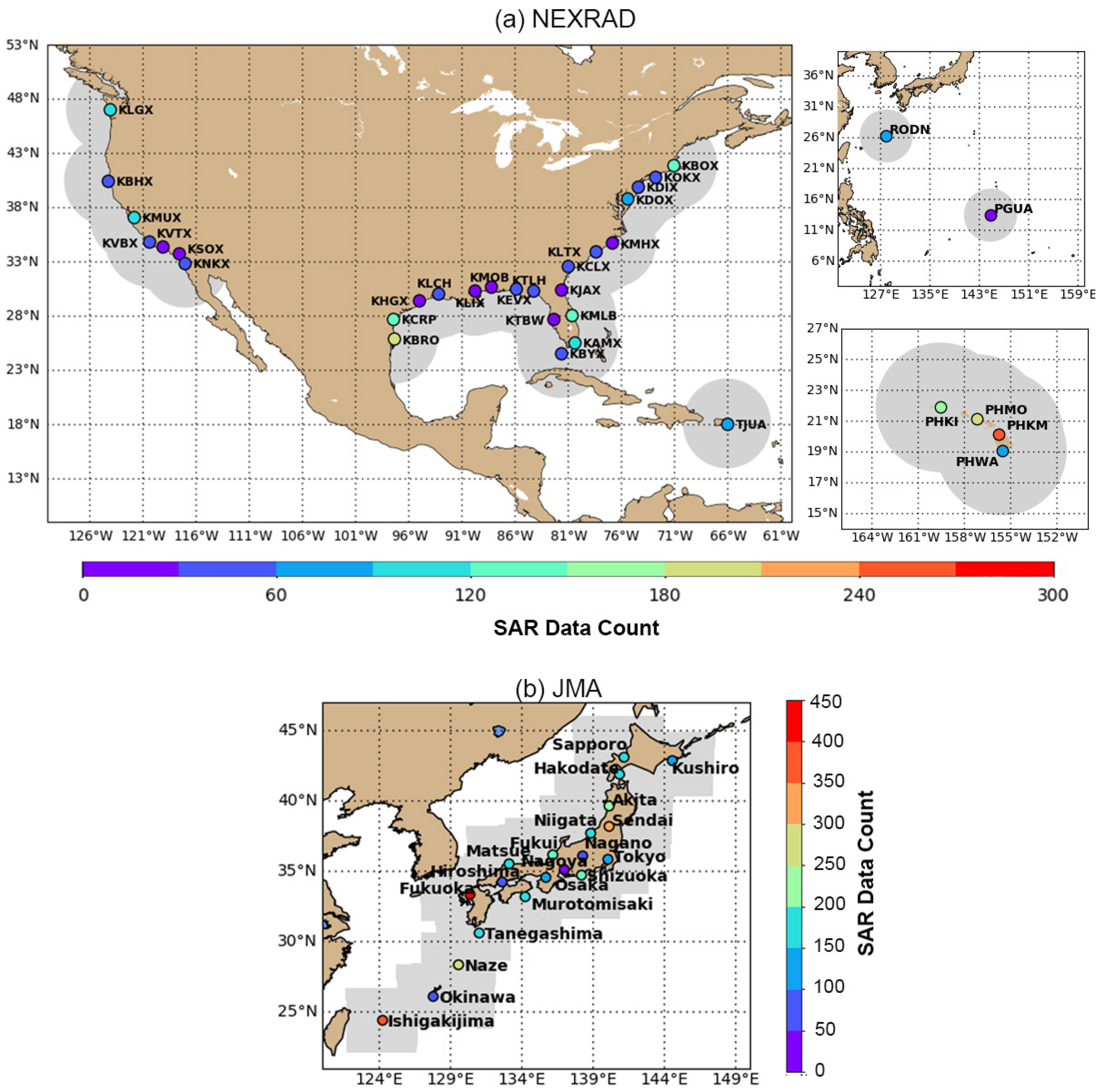
We use two different networks. The NOAA network is mainly used to document the impact of rain on NRCS and to develop the detection method. We rely on data from the JMA network for independent validation. The location and coverage of the coastal radars from NOAA and JMA are shown in Figure 1.

The NOAA network is called Next Generation Weather Radar (NEXRAD) network, which consists of 159 S-band high-resolution weather radars throughout the United States and several overseas locations. A total of 34 stations are distributed in the coastal area, as shown in Figure 1a. NEXRAD provides different precipitation products, including base reflectivity (1 km/5 min), base velocity (1 km/5 min), one-hour precipitation (1 km/1 h) and hydrometeor classification (0.25 km/5 min). In this paper, we rely on the base reflectivity instead of one-hour precipitation for rain intensity reference because of its high temporal resolution and its larger coverage. The base reflectivity is an indicator of rain intensity, which is usually used to derive rain rate by classical Marshall-Palmer conversion [27]. It is a radar station centered product with a radius of 460 km acquired with a 0.5${}^{\circ }$ elevation angle. Please note that the radar beam altitude increases with the distance from radar station to reach more than 10 km at the edge of radar coverage.

The rain rate provided by JMA has 1 km resolution every 10 min on a single grid and covers the full Japanese archipelago. The product is based on constant altitude plan position indicator (CAPPI) reflectivity data at about 2 km altitude from multiple JMA radars. Rainfall rate (mm/h) is estimated from reflectivity values (dBZ) using a reflectivity-rainfall (Z-R) relationship of Marshall and Palmer [27].

2.3. Match-Up Database with Sentinel-1 and Weather Radar Data

A match-up step is necessary for the following analysis because both data have different temporal and geographic coverage. Additionally, because rain can have a strong variability, assessing its impact on high-resolution products such as a SAR image requires severe criteria in both space and time. First, Sentinel-1 data are matched up with weather radar coverage. Secondly, for each Sentinel-1 case, we select the nearest weather radar observations in time. The maximum temporal difference between the satellite and weather radar is set to 5 min. Finally, the rain data at 1 km resolution are mapped on the same grid as Sentinel-1 products by searching the nearest neighbor in weather radar map. Please note that the Sentinel-1 products in Section 3 is degraded to 1 km. But in Section 4, the original resolution (5 m by 20 m) in IW mode was reduced to 200 m, 400 m, 800 m as applying the dual-polarization filter.

Note, although we benefit here from high-resolution rain measurements and high frequency sampling (with respect to any low-orbit satellite mission), this collocation strategy is not perfect. As pointed out by Melsheimer et al. [23], there is a time difference between the time when the rain is observed by the ground-based radar and the time when the raindrops hit the sea surface. This difference depends on the distance of the observed rain event, the altitude and height of the water column as well as on the rainfall speed. For instance, for a rainfall speed of 6 to 8 m/s observed at a height of 4 km, scattering effect due to raindrops impinging the surface are expected to be observed at least 10 min later. However, as rain fall speed and sizes are not known here, for each SAR scene we simply select the weather radar observation in the shortest time lag. In addition, Melsheimer et al. [23] pointed out that wave damping effect due to rain-generated turbulence may occur after the rainfall has stopped, inducing another time lag, which can contribute to collocation errors, but is very difficult to quantify. The spatial extent of the rain signature between the two sensors is also expected to be different for storm cells because the downdraft area is not visible on the ground-based rain radar. Finally, from our experience and as illustrated hereinafter, the correlation between the two nearest measurements in time is remarkable. After collocation, we restrict the match-up data pairs to rainy situations. We finally obtained a total of 2393 and 4311 S-1 images co-located with NEXRAD and JMA observations, respectively.

Additionally, considering that ocean surface winds have a direct influence on sea surface roughness and consequently on the SAR backscattered signal, we also collocated the measurements with hourly forecast wind products provided by European Centre for Medium Range Weather Forecasts (ECMWF). They are available on a spatial grid of 0.125${}^{\circ }$ limiting the time difference with the observations to 30 min.

3. Co-Analysis of Rain Rate and C-Band SAR Backscattering

3.1. A First Qualitative Assessment

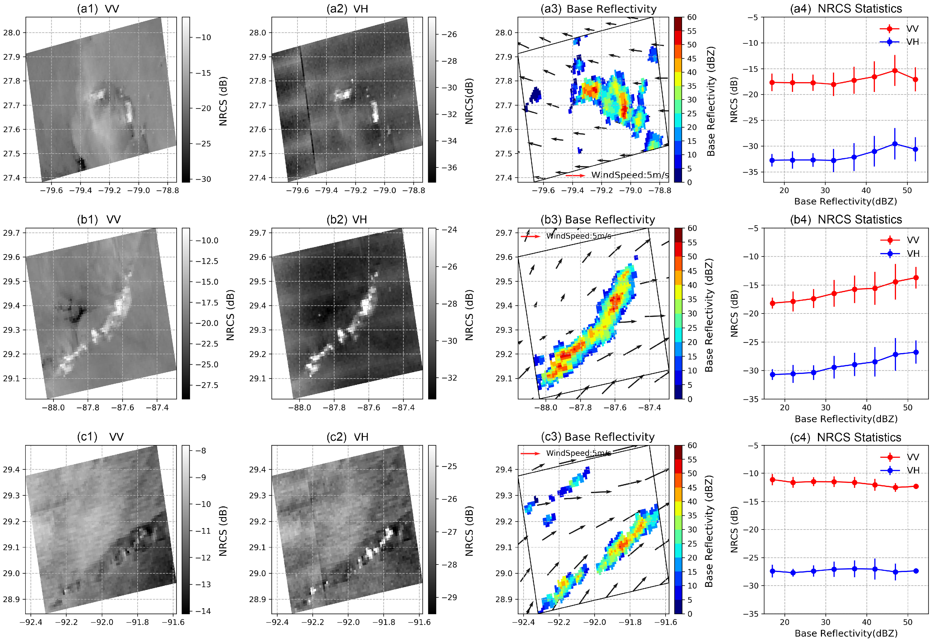
Different forms of rain exist in nature, such as rain cells, stratified rain, rain bands or squall lines. The nature of hydrometeors (type, size, distribution in the atmosphere column) and local effect on the ambient wind are different in these rain forms leading to different signatures on C-band SAR images. This variety is illustrated with three examples in Figure 2:

• Case a (Top in Figure 2): This is a typical example of storm cell footprint as discussed by Atlas [28]. Both VV- and VH-polarized images show two rain areas with concurrent bright and dark patches within the cell, the downdraft area and the wind gust. Here the surrounding wind speed is about 3 m/s. Collocated NEXRAD measurements presented in Figure 2(a3) indicate two separate rain cells. Bright patches are located at the same location in VV and VH images and correspond to NEXRAD base reflectivity measurements higher than 40 dBZ. This suggests an increase of C-band radar backscattering at high rain rates. As also noted by Melsheimer et al. [23], the extent of base reflectivity is less than the storm cell signature in the SAR image as rain radar is not sensitive to the wind acceleration due to downdraft or its associated wind gust. In this case, the relationship between NRCS and base reflectivity confirms the NRCS increases with base reflectivity for values larger than 40 dBZ.
• Case b (Middle in Figure 2): This case acquired in the Gulf of Mexico corresponds to a stationary front with stratiform precipitation without intense vertical convection. As indicated by Figure 2(b3), wind speed is significantly different on each side of the atmospheric front with ambient background wind speed lower than 2 m/s in the western area and higher than 6 m/s in the eastern area. In this case, there is also a good match between bright patches observed on both co- and cross-polarization channels and the highest values of base reflectivity (see Figure 2(b3)). The relationship between NRCS and base reflectivity also confirms that for values larger than 25 dBZ, the NRCS increases with base reflectivity.
• Case c (Bottom in Figure 2): Here, the background ambient wind is stronger than in the previous cases, about 13 m/s from the model. As observed, the distribution, size and intensity of the bright patches are not the same in co- and cross-polarization. More bright patches are observed in VH than in VV. In particular, dark areas are observed in the VV image where the VH image exhibits bright patches associated with high base reflectivity. As a result, in this case, the VV NRCS shows decreases when the base reflectivity increases whereas the VH NRCS stays almost constant.

As confirmed by these examples, the impact of rain on co- and cross-polarization NRCS at C-band is quite complex and depends on both rain rate, ambient sea state and polarization.

3.2. Timeliness of the Data

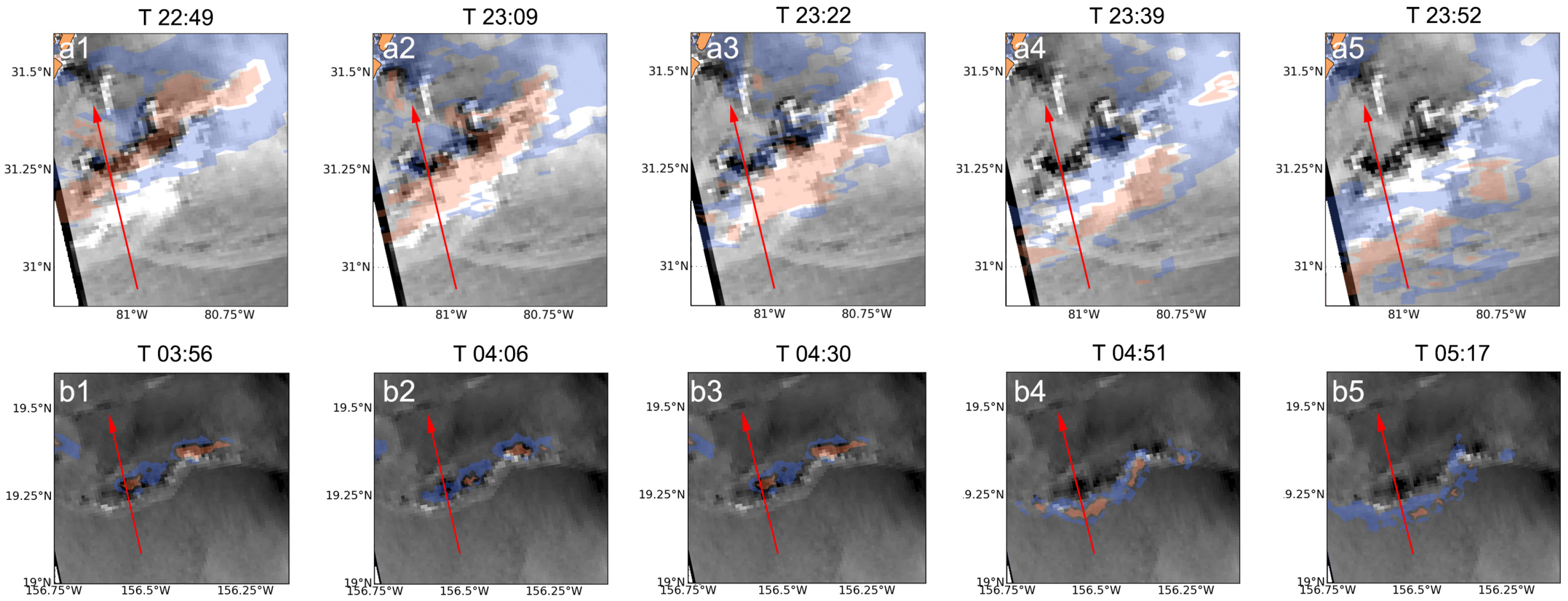
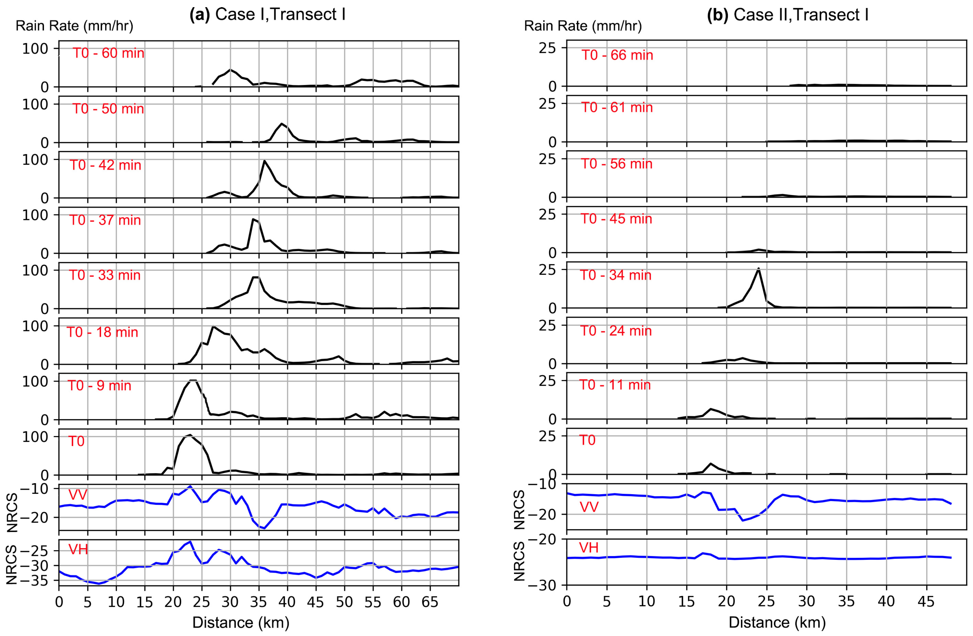
As explained in Section 2, we selected the rain data with the closest time to each Sentinel-1 case. The timeliness of the two datasets is very important and may be decisive for efficient training when preparing the reference dataset since the rain cells can have an apparent shift up to several minutes. In particular, the rain splash and ring waves are triggered immediately by raindrops but the wave damping is expected to be maximum after the rain event. Figure 3 and Figure 4 illustrate this point. In Figure 3, two different rain events are considered. The image in VV polarization is plotted along with the base reflectivity corresponding to different times before (a1–a2 and b1–b2) and after (a4–a5 and b4–b5) the acquisition time (a3 and b3). For a given transect across these two images (red line), the NRCS values for co- and cross-polarization are plotted together with the base reflectivity measured at different times around the SAR data acquisition. For each case, we observe a high negative correlation between the rain rate and the NRCS value at about 30 min (see Figure 4 before SAR acquisition time). Please note that for these two cases, we only observed the decrease in the co-polarized channel so that only VV-polarized images are presented in Figure 3. Here, the decrease cannot be attributed to attenuation of the radar signal by rain in the atmosphere, since the dark area is in front of the bright area with respect to the antenna look angle. This indicates that the rain occurring 30 min before the SAR data acquisition has generated turbulence. In addition, the maximum rain rate is observed at the SAR acquisition time, which is coincident with the enhanced NRCS in the SAR images. This observation suggests that NRCS enhancement is related to surface scattering at rain-generated splash products [18] or backscattering in the atmosphere [21]. The information of hydrometeor classification provided by NEXRAD network could help to classify this effect, which shall be discussed next.

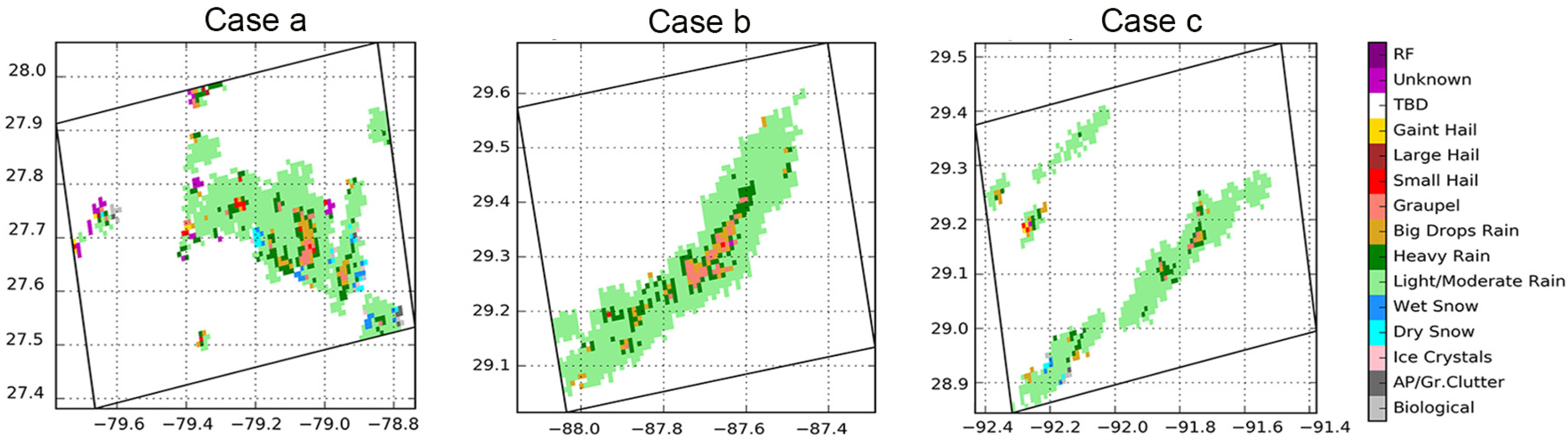
3.3. Scattering by the Melting Layer

There is no doubt that the rain-induced structures (ring waves and splash products) can enhance the sea surface roughness in low to moderate wind regimes as illustrated by the experiments conducted by Moore et al. [29], Bliven et al. [30] and Braun and Gade [18]. However, for SAR operating on spacecraft, the signal transmission in the atmosphere (not considered in the laboratory experiments) can not be neglected since rain/hydrometeors can scatter and absorb part of the microwave energy. By taking advantage of the observations from multi-sensors and/or at multi-polarizations, Jameson et al. [31], Katsaros et al. [32] and Alpers et al. [21] attribute the strong and localized enhancement of NRCS values to radar backscattering hydrometeors in the melting layer, where the falling ice particles undergo phase change from solid to liquid. Here, we provide more evidence for the contribution from hydrometeor in the melting layer in Figure 5. This figure presents the hydrometeor classification corresponding to the three rain events of Figure 2. The product of hydrometeor classification is provided by NEXRAD for an elevation angle of 0.5° (around 4–5 km where the rain cells are located). It shows that most of the rain-related features in the SAR image correspond to pixels for which the classification indicates light/moderate rain. However, the brightest patches (corresponding to highest NRCS values) in VV and VH seem to be strongly associated with radar backscattering from graupel/hail. Moreover the presence of graupel/hail, big drop rains validated the presence of the melting layer. As investigated by Browne and Robinson [33] and Jameson [34], the cross-polarized backscatter was found with more contribution from the melting layer than the co-polarized one. These high correlations found between the dual-pol images and the classification further confirm the importance of the melting layer in the strong backscatter observed in C-band SAR images acquired during events.

3.4. Statistical Analysis

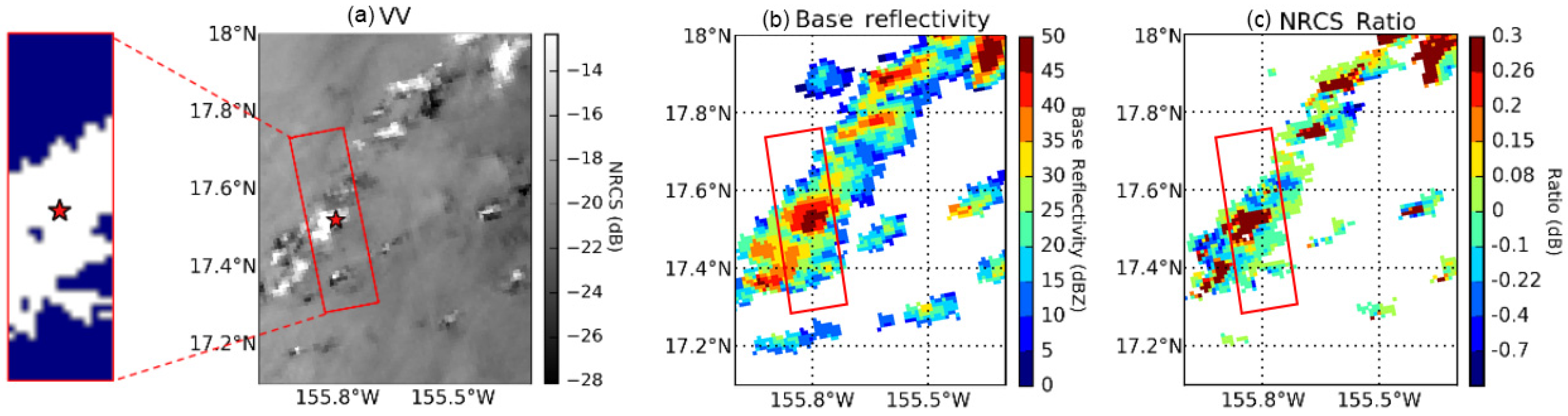
To further document the effective rain impact, we follow methodology from Braun and Gade [18] and rely on the ${\mathrm{NRCS}}_{\mathrm{ratio}}$ quantity, defined as the ratio of NRCS from rainy area over the NRCS from the sea surface in the surrounding area without rain as indicated by the rain radar:

$${\mathrm{NRCS}}_{\mathrm{ratio}}=10{log}_{10}\frac{{\mathrm{NRCS}}_{\mathrm{rain}}}{{\mathrm{NRCS}}_{\mathrm{rain}-\mathrm{free}}}\mathrm{with}\left\{\begin{array}{cc}\mathrm{rain}\hfill & \mathrm{if}Z\ge Z_0\hfill \\ \mathrm{rain}-\mathrm{free}\hfill & \mathrm{if}Z<Z_0\hfill \end{array}\right.$$

(1)

where Z is the base reflectivity (in dBZ) measured by NEXRAD and $Z_0$ the threshold to define rain-free area. $Z_0=20\mathrm{dBZ}$ hereinafter. The threshold of 20 dBZ usually indicates the falling precipitation according to the National Oceanic and Atmospheric Administration (NOAA). The ${\mathrm{NRCS}}_{\mathrm{ratio}}$ value indicates how much NRCS increases or decreases with rainfall in comparison to rain-free sea surface area, assuming a multiplicative effect on the backscattering intensities in linear scale. To account for the joint effect of local incidence angle and sea state, this variable is computed locally as illustrated in Figure 6.

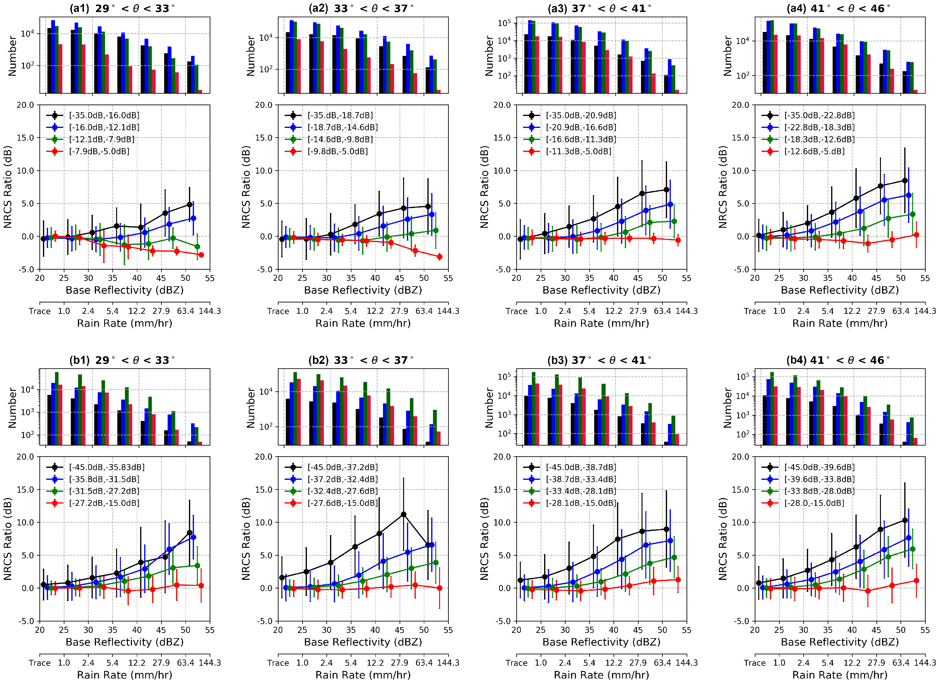
We have split the entire S-1/NEXRAD database into four ranges of incidence angles angle bins to analyze the ${\mathrm{NRCS}}_{\mathrm{ratio}}$. The incidence angle intervals are 29${}^{\circ }$–33${}^{\circ }$, 33${}^{\circ }$–37${}^{\circ }$, 37${}^{\circ }$–41${}^{\circ }$ and 41${}^{\circ }$–46${}^{\circ }$. Figure 7 displays the statistics of ${\mathrm{NRCS}}_{\mathrm{ratio}}$ as a function of base reflectivity with 5 dBZ bins. For convenience, we have also converted the NEXRAD base reflectivity into rain rate using the conversion ${\mathrm{Z}}_{\mathrm{lin}}=300{\mathrm{R}}^{1.4}$ [35], where ${\mathrm{Z}}_{\mathrm{lin}}$ is not in dBZ, but in linear scale. First and second rows show the results for VV and VH polarizations, respectively. In addition, for each range of base reflectivity, the ${\mathrm{NRCS}}_{\mathrm{ratio}}$ is analyzed for different ranges of ${\mathrm{NRCS}}_{\mathrm{rain}-\mathrm{free}}$ as a proxy of the wind speed condition. As expected from our ratio computation method, the ratio tends toward 0 when the rain rate tends toward the threshold used for rain-free areas ($Z_0=20\mathrm{dBZ}$).

For VV polarization, at low to moderate winds (<16 m/s), the ${\mathrm{NRCS}}_{\mathrm{ratio}}$ shows an increasing trend with rain rate at all incidence angles except as wind speed exceeds 8 m/s with incidence angle lower than 33${}^{\circ }$. Overall, these results conform with results obtained by Moore et al. [29] and Lin et al. [22]. The mean ${\mathrm{NRCS}}_{\mathrm{ratio}}$ values are found to be positive excepted for low winds (black lines corresponding to lowest values of NRCS without rain) and light rain (base reflectivity lower than 25 dBZ) for which the ratio is found to be around zero. This is different from statistical analysis carried out by Lin et al. [22] scatterometer data from ASCAT, which shows a significant increase of the NRCS even for very light rain. However, the ASCAT scatterometer (as well as microwave radiometers) have resolution of tens of kilometers, whereas the statistics in this study is at a resolution of 1 km. Neglecting the atmosphere attenuation effect (reasonable for light rain at C-band), we anticipate the negative ${\mathrm{NRCS}}_{\mathrm{ratio}}$ values reveal the localized effect of small-scales surface waves damping under light-to-medium rain rate. Because the data are in high resolution, this effect is not counterbalanced by wind sea from ambient wind or downdraft winds as is most likely the case for lower-resolution data.

For wind speeds larger than 16 m/s (see red lines), the ${\mathrm{NRCS}}_{\mathrm{ratio}}$ values are negative and almost constant in comparison with lower wind speeds. ${\mathrm{NRCS}}_{\mathrm{ratio}}$ even exhibits a slight decrease for incidence angles lower than 37${}^{\circ }$. Additionally, it is noted that the ${\mathrm{NRCS}}_{\mathrm{ratio}}$ fluctuates around zero for wind speed of 8–16 m/s as incidence angle lower than 33${}^{\circ }$. First, the decrease in sensitivity to rainfall in the C-band radar backscattering results from the competing effect of rain to change (mostly increasing) the NRCS and the background sea-state contribution. For stronger winds and severe sea state, the wind-waves already saturate the centimeter scales ocean surface waves and breaking waves become significant. In these conditions, rain-induced phenomena such as ring waves and splash products can hardly contribute to increasing the surface roughness and even probably contribute by smoothing the surface. This smoothing effect is pronounced at low incidence angle even though the wind speed is not that strong at a low incidence angle (See green line in Figure 7(a1)). Secondly, possible attenuation from the atmosphere can also add to the negative ${\mathrm{NRCS}}_{\mathrm{ratio}}$ values. Please note that except for the lower incidence angle range, the ratio is for intermediate wind speeds (green lines) close to zero or negative for rain rates lower than 30 dBZ before it increases for larger rain rates. For given wind speed and base reflectivity, the ${\mathrm{NRCS}}_{\mathrm{ratio}}$ increases with incidence angle. Rain signatures are thus expected to be larger at cross-polarization for large incidence angles than at co-polarization.

Compared to co-polarization, few studies exist on rain signatures at cross-polarization. Case studies analyzed by Melsheimer et al. [14], Vachon and Wolfe [36] and Mouche and Chapron [37], show that the rain signatures at cross-polarization might be more pronounced than at co-polarization. As for VH, the ${\mathrm{NRCS}}_{\mathrm{ratio}}$ statistics of VH-polarized images are presented in Figure 7(b1–b4). For light rain and low NRCS values (corresponding to light wind speeds), the ${\mathrm{NRCS}}_{\mathrm{ratio}}$ values at cross-polarization are found to be significantly higher than in co-polarization. However, the signal-to-noise ratio is very low in cross-polarization and noise contamination impact cannot be excluded for this particular regime. Apart from this, the ${\mathrm{NRCS}}_{\mathrm{ratio}}$ values are found to increase with base reflectivity for all wind speed regimes considered in this study. This sensitivity decreases with increasing wind speed. For a given base reflectivity, our analysis does not reveal a clear dependency of ${\mathrm{NRCS}}_{\mathrm{ratio}}$ on incidence angle. This is explained by the fact that the cross-polarization backscattered signal from the ocean surface is much less sensitive to incidence angle than at co-polarization [36]. This suggests that rain signature should not be incidence angle dependent in cross-polarization.

Overall, above statistics indicate that VH is more sensitive to rain than VV for the whole range of incidence angle and wind speed considered in this study. At VV channel, the ${\mathrm{NRCS}}_{\mathrm{ratio}}$ values are likely to be negative for strong wind speeds, leading to apparent darker features at VV than at VH with respect to the background NRCS. This is in line with the third case study presented in Figure 2. The sensitivity to rain is also found to be incidence angle dependent in VV as opposed to VH. This suggests less impact of rain at low incidence angles in VV.

In addition to assessing the mean behavior for the NRCS during rain events, our study also confirms a significant variability around the averaged trend (see vertical bars in Figure 7). The two main reasons are the possible temporal mismatch between the satellite and the ground-based radar, as well as the extreme variability of the rain features observed, which might include adjacent dark and bright areas(areas of increased as well as of decreased NRCS values relative to the background) as illustrated in Figure 2. For VV polarization, at low to moderate winds (<16 m/s), the ${\mathrm{NRCS}}_{\mathrm{ratio}}$ shows an increasing trend with rain rate at all incidence angles. Overall, these results are coincident with previous studies of Moore et al. [29] and Lin et al. [22]. The mean ${\mathrm{NRCS}}_{\mathrm{ratio}}$ values are found to be positive excepted for high winds.

4. Rain Detection

In the previous section, we have outlined the large variability of the rain signatures on C-band SAR co- and cross-polarized images with respect to incidence angle and to some extent to the underlying sea state. Due to the variety of rain-induced features, a simple methodology solely based on thresholds and NRCS intensities values may not be satisfactory enough. In the following, we thus consider textural information to attempt the detection and segmentation of rain on sea surface SAR images.

4.1. Optimization of the Heterogeneity Filter(s) for Rain Detection

The local gradient method is proposed by Koch [25] to detect heterogeneity across SAR images, which has the capability of locating multiple objects, such as land areas, fronts, oil spills, ships, even under non-uniform ocean environment conditions. To filter out small-scale ocean features and speckle noise, we first reduce the spatial resolution and thus smooth the image. Speckle noise is inherent to SAR images due to the coherent processing of radar signals. Our analysis requires further speckle noise reduction even though the speckle noise has already been decreased in ground-detected SAR images by applying multi-look SAR processing (the Equivalent Number of Looks for the Sentinel-1 IW SAR mode is 4.4). In addition to rain signatures, SAR images acquired over sea surface may include other small-scale features with scales of meters to decameters (e.g., waves) which are out of the scope of this study. In this study, we use three resolutions (200 m, 400 m and 800 m) in the analysis of co- and cross-pol Sentinel-1 SAR images to eliminate the wave impact with wavelengths on the order of 100 m. Following the study in Koch [25], we compute four parameters (denoted $P_i$):

• $P_1$: The ratio between the standard deviation and the average computed for each pixel using a sliding bounding box of the smoothed/reduced image. It is computed using a convolutive averaging bounding box over the amplitude (square root of NRCS) and its second moment. This parameter is particularly useful to decipher open water surface from other extended areas (land, tidal zones, sea ice, etc.)
• $P_2$: The second parameter is built on a Laplace pyramid filter with the difference between images at adjacent levels in the pyramid. It is based on the squared ratio of the high-pass-filtered image and its local average. It has the capability of detecting narrow image features, as slicks, internal waves, or fronts.
• $P_3$: The third parameter is the ratio of the magnitude of the squared local Sobel-based gradient and its local average. A Sobel operator is basically involved to do spatial gradient measurement on 2-dimensional images. It is generally adapted to detect edges and point targets.
• $P_4$: The ratio between the reduced/smoothed version of the squared local gradient and its absolute squared gradient: it can be considered to be a measure of directional coherence. It should detect the edges such as ”slicks, internal waves, or fronts” [25].

In study of Koch [25], these four parameters are studied via a histogram analysis to optimize the separability between wind and non-wind related features, which he termed heterogeneous areas. They are linearly scaled between 0 and 1, leading to the four parameters $f_i$. In this study we adapt these 4 parameters for rain detection, although they applied them to co-polarized ERS-1/-2 SAR images. The squared average of linearly scaled $f_i$ parameters is then computed, leading to a single F parameter ranging from 0 and 1.

$$F=\sqrt{\frac{1}{4}\sum _{i=1}^4{f}_i^2}$$

(2)

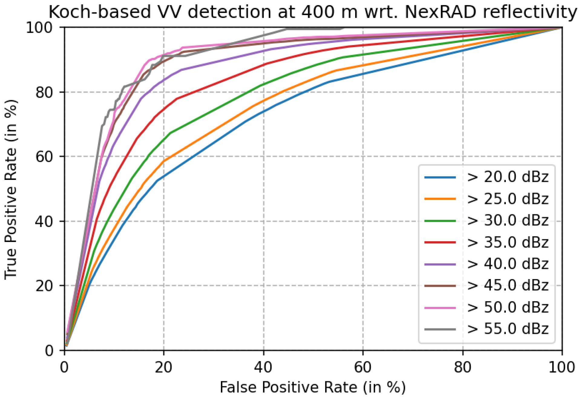
At this stage, this parameter is calculated at different resolutions r ($r=\{200,400,800\}$) and for the two polarization channels p ($p=\{\mathrm{VV},\mathrm{VH}\}$), hereafter denoted $F_{r,p}$. In Koch [25], a single threshold is applied to F to indicate the presence of heterogeneity (set as 0.6 for all proposed resolutions—ERS-1 only has single-polarization capabilities). Several quantitative indices/criteria can be employed to assess the goodness-of-fit between the rainy area provided by the reference rain mask and the $F_{r,p}$ parameter. Applying a specific threshold $F_{r,p}>{\nu }_{r,p}$ with ${\nu }_{r,p}=[0,1]$ would enable a direct comparison between two binary masks with Dice coefficient or Intersection over Union (IoU) indices. An analysis based on Receiver Operating Characteristic (ROC) curve is outlined in Figure 8 with $r=400$ and $p=VV$. The ROC is based on the analysis of True Positive Rate (TPR) and False Positive Rate (FPR) for varying ${\nu }_{r,p}=[0,1]$. We recall that TPR is the proportion of S-1 heterogeneous area in the S-1 SAR images that is correctly predicted out of all heterogeneous observations (based on a given rain flag reference from NEXRAD). Similarly, FPR is the proportion of S-1 observations that are incorrectly predicted as heterogeneous out of all homogeneous observations.

$$\begin{array}{cc}\hfill \mathrm{TPR}\left({\nu }_{r,p}\right)& =\frac{|F_{r,p}>{\nu }_{r,p}|\cap |Z>Z_0|}{|Z>Z_0|}\hfill \\ \hfill \mathrm{FPR}\left({\nu }_{r,p}\right)& =\frac{|F_{r,p}>{\nu }_{r,p}|-|F_{r,p}>{\nu }_{r,p}|\cap |Z>Z_0|}{|Z>Z_0|}\hfill \end{array}$$

Here $|.|$ denotes the cardinality of a given set, which is the number of pixels of the set in the database.

Figure 8 shows that the Koch filter improves with the rain rate increasing. It is remarkable that TPR reaches 90% with low FPR of 20% when considering Z₀ = 45 dBZ region (equivalent to 24 mm/h). In contrast, for the same value of TPR, FPR increases up 70% when the rain rate decreases below 30 dBZ (equivalent to 1 mm/h). It is expected that co-polarized SAR images show bright patches for base reflectivity exceeding 40 dBZ (see previous section, whereas the backscatter is dominated by sea surface winds especially at light rain).

To find the best trade-off between FPR and TPR (and hence the optimal ${\nu }_{r,p}^{opt}$), the minimum distance from the ROC curve to the top left corner is calculated as proposed by Tilbury et al. [38]. An alternative method is to calculate the maximum of the Youden index [39].

$${\nu }_{r,p}^{opt}=\mathrm{argmin}\sqrt{{\left(1-\mathrm{TPR}\left({\nu }_{r,p}\right)\right)}^2+\mathrm{FPR}{\left({\nu }_{r,p}\right)}^2}$$

(3)

For $r=400$ and $p=\mathrm{VV}$, ${\nu }_{400,VV}^{opt}$ is found to be equal to about 0.78 independently of the $Z_0$ value. Beyond this first analysis, it is also of interest to investigate the potential to combine different resolutions and/or polarization channels. To this end, the same assessment based on ROC curves is extended, where the final heterogeneity mask is the intersection of each individual heterogeneity mask. All the possible pairs of processing ($r=\{200,400,800\}$ and $p=\{\mathrm{VV},\mathrm{VH}\}$) are combined with a joint optimization of the two individual thresholds ${\nu }_{r1,p1}^{opt}$ and ${\nu }_{r2,p2}^{opt}$ ($r1,r2$∈ {200, 400, 800}, $p1,p2$∈$\{\mathrm{VV},\mathrm{VH}\}$ ).

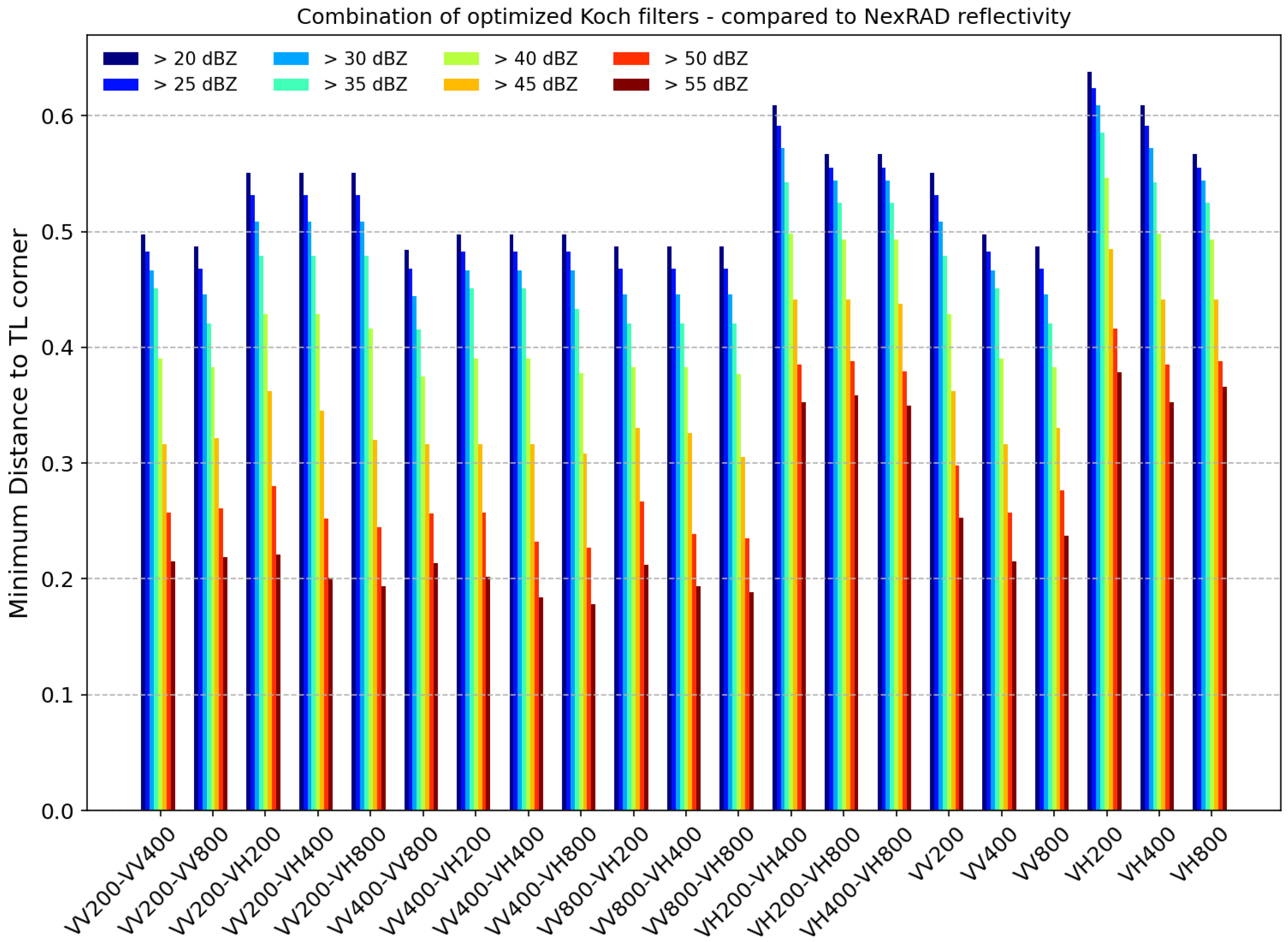
In Figure 9, the minimum distance to the top left corner is retained as criteria (similar results are obtained with the Youden Index—not shown here) and estimated for 5 intervals of rain rates (Z ranges from 20 to 55 dBZ). Figure 9 shows the following: The filters based on co-polarized NRCS values are significantly better than the ones based on cross-polarized NRCS values. One possible explanation is that the signal-to-noise ratio at cross-polarization is much lower than at co-polarization. Indeed, this can prevent to detect the texture modification in some cases. A striking example of the noise impact in the case of two storm cells observed by Sentinel-1A C-band SAR is presented in Figures 5 and 6 in Alpers et al. [17]. As observed, several storm cell related features are not visible in cross-polarization images, but in co-polarization images. $F_{400,VV}$ filter provides the best agreement when only one filter is chosen. Thus, combining co- and cross-polarization information improves the detection performance. Among all the possibilities, the joint $\left(F_{400,VV};F_{800,VH}\right)$ filter exhibits the best agreement with observations with weather radars. The optimized thresholds are ${\nu }_{400,VV}^{opt}=0.78$ and ${\nu }_{800,VH}^{opt}=0.71$. We refer to the filter obtained by combining both co- and cross-polarization channels as dual-pol filter hereafter.

4.2. Validation of the Performance of the Filters

The computation of the filter has been applied to all available Sentinel-1 data collocated with JMA rain measurements to assess rain detection performance with respect to the choice of polarization channels, incidence angle and wind speed. Here wind speed is used as a proxy of the local sea state. Three different polarization configurations are considered: The joint $\left(F_{400,VV};F_{800,VH}\right)$ filter and one for each polarization channel the $F_{400,VV}$ and $F_{800,VH}$ filters.

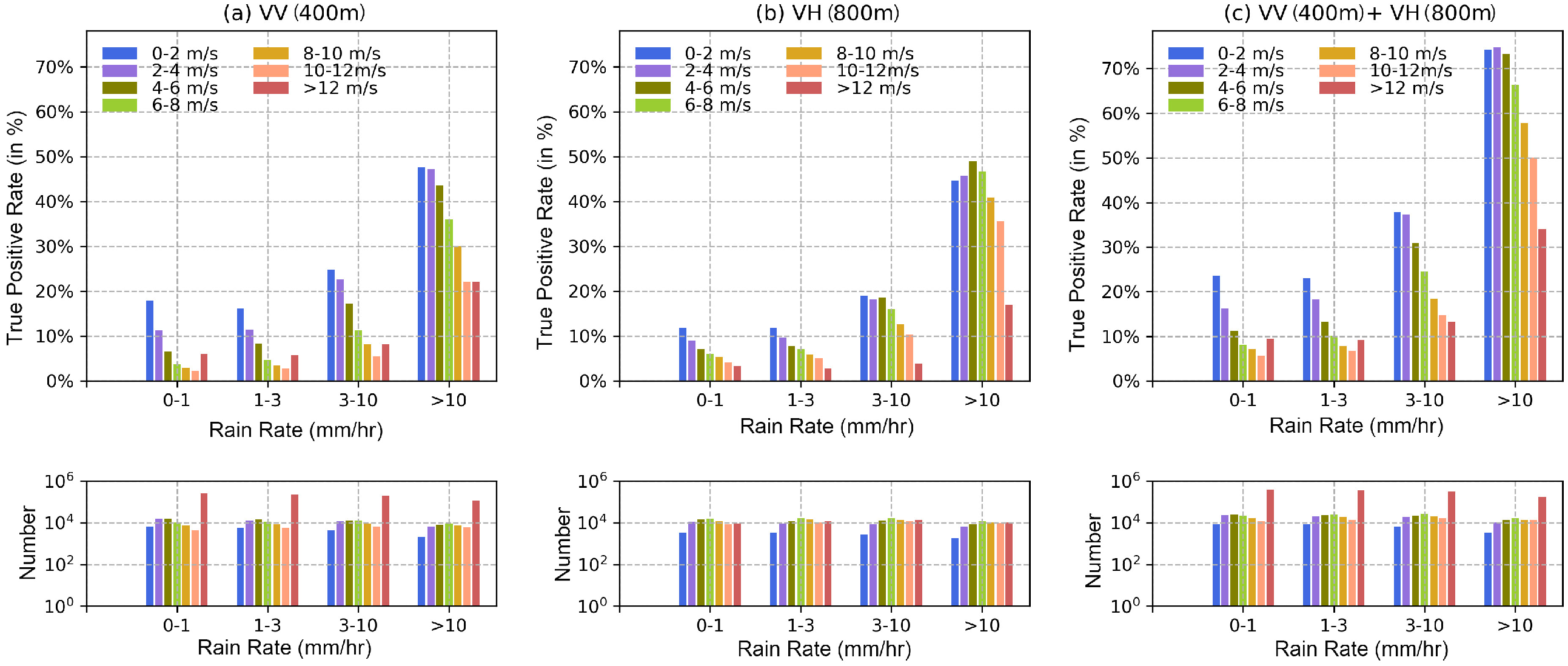
Figure 10 shows the rain detection percentage as a function of rain rate for different wind speed regimes with respect to the polarization channels considered for the detection. As observed, no matter the polarization configuration, rain is more likely detected when the rain rate is high. For all rain rate regimes, the background sea state is found to have an impact on the detection. For a given rain rate, the higher the wind speed, the less we can detect rain in the signal. In particular, for rain rates larger than 10 mm/h, the detection rate increases significantly when the wind speed decreases. Furthermore, the benefit of merging the two polarization channels for rain detection is evident, since the percentage of rain detected pixels increases from about 20–50% to up to $70\%$ when both co- and cross-polarization channels are combined.

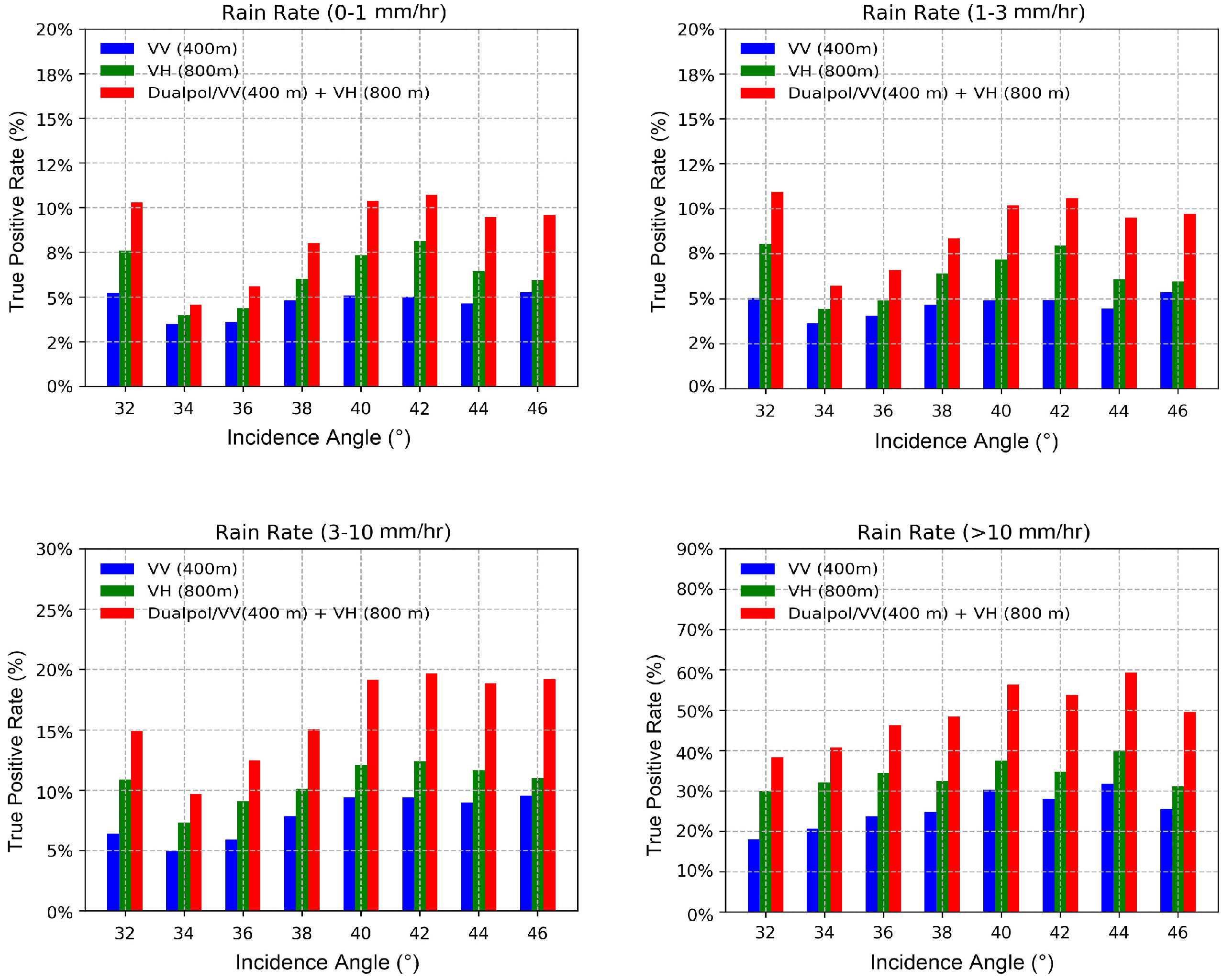
Figure 11 shows the detection rate as a function of incidence angle for different rain rates. It shows that the rain detection increases with incidence angle independent of the applied heterogeneity filter. These results confirm that C-band SAR measurements are more sensitive to rain for high incidence angles as documented in Section 3.

In general, the higher detection rate of rain obtained when the two polarizations are combined show their complementary. This suggests that the different sensitivity of the co- and cross-polarization channels to rain rate could be due to different scattering mechanisms.

4.3. Application of Dual-Pol Filter on Different Rain Types

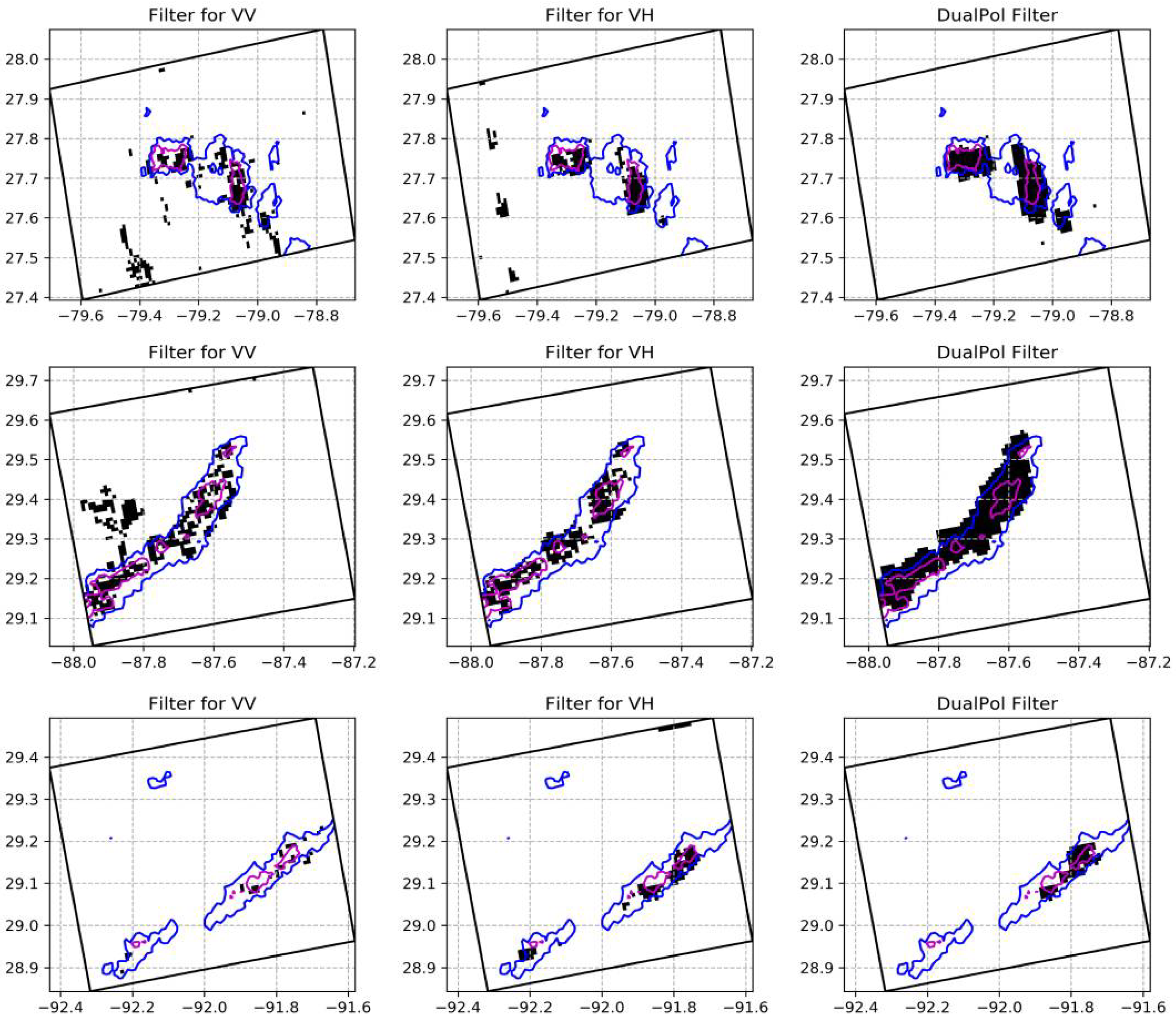
The application of the dual-pol filter on the three cases in Figure 2 is shown in Figure 12, where the filters generated with VV (400 m), VH (800 m) and dual-polarizations channels are included. Here the blue and purple contours indicate the base reflectivity of 20 dBZ and 40 dBZ as given by the NEXRAD weather radar. In these cases, the dual-pol filter clearly shows a better agreement with NEXRAD data, in particular as reflectivity is larger than 40 dBZ. As shown for the first case, it seems that the VH filter is more sensitive to noise than the VV and dual-pol filters as demonstrated by the subswath jump and the modulation in the azimuthal direction on the left-hand side of the swath at low incidence angle. Furthermore, VV filters seem to capture signatures that do not correspond to high base reflectivity values such as the wind gust front on the first case and the area with low backscattered signal observed on the second case. The third case is more complex. VH and VV signatures have opposite signs and only the VH filter (positive rain signature) can capture the rain signature in the south area. The areas with the strongest rain rate are captured by all three filters. These three cases illustrate the capabilities of the dual-polarization for filtering rain signatures.

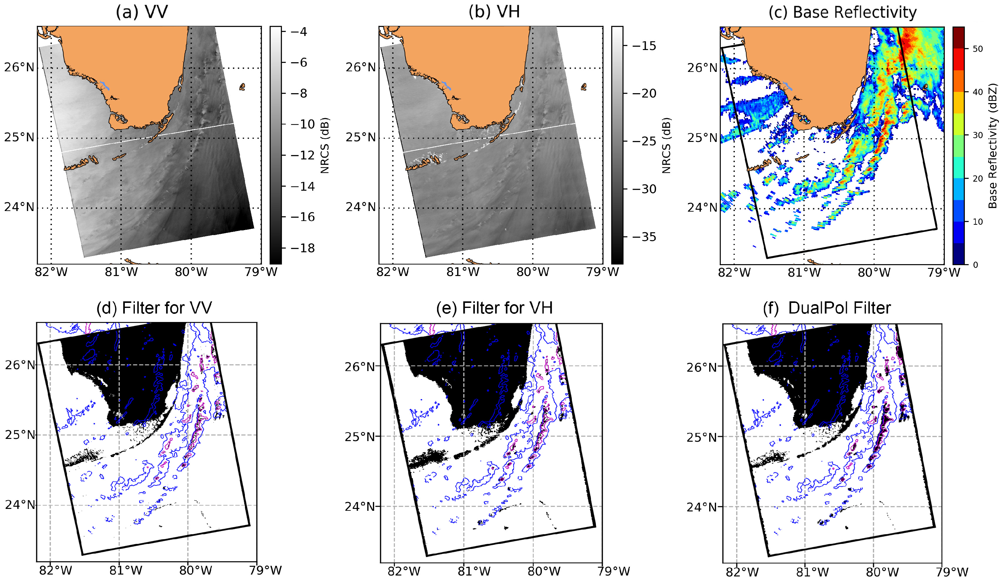
Tropical cyclones or strong storms such as extra-tropical cyclones, polar lows and medicanes are other phenomena in which the question of discriminating between rain and background sea state remains. Figure 13a,b show S-1 images for both VV and VH polarizations in the case of Irma tropical cyclone, when the eye was over Florida. Figure 13c is the corresponding base reflectivity as measured by the ground-based radar from NEXRAD network. Here the wind speed is larger than 30 m/s (larger than in our present study) and the base reflectivity is larger than 48 dBZ. As observed in Figure 13f, when applied to such an extreme case, the dual-pol filter can detect the main areas impacted by rain and certainly helps improve the quality of wind estimates in such complex situations. However, further analysis remains to be done for a proper assessment of our method in those extreme situations.

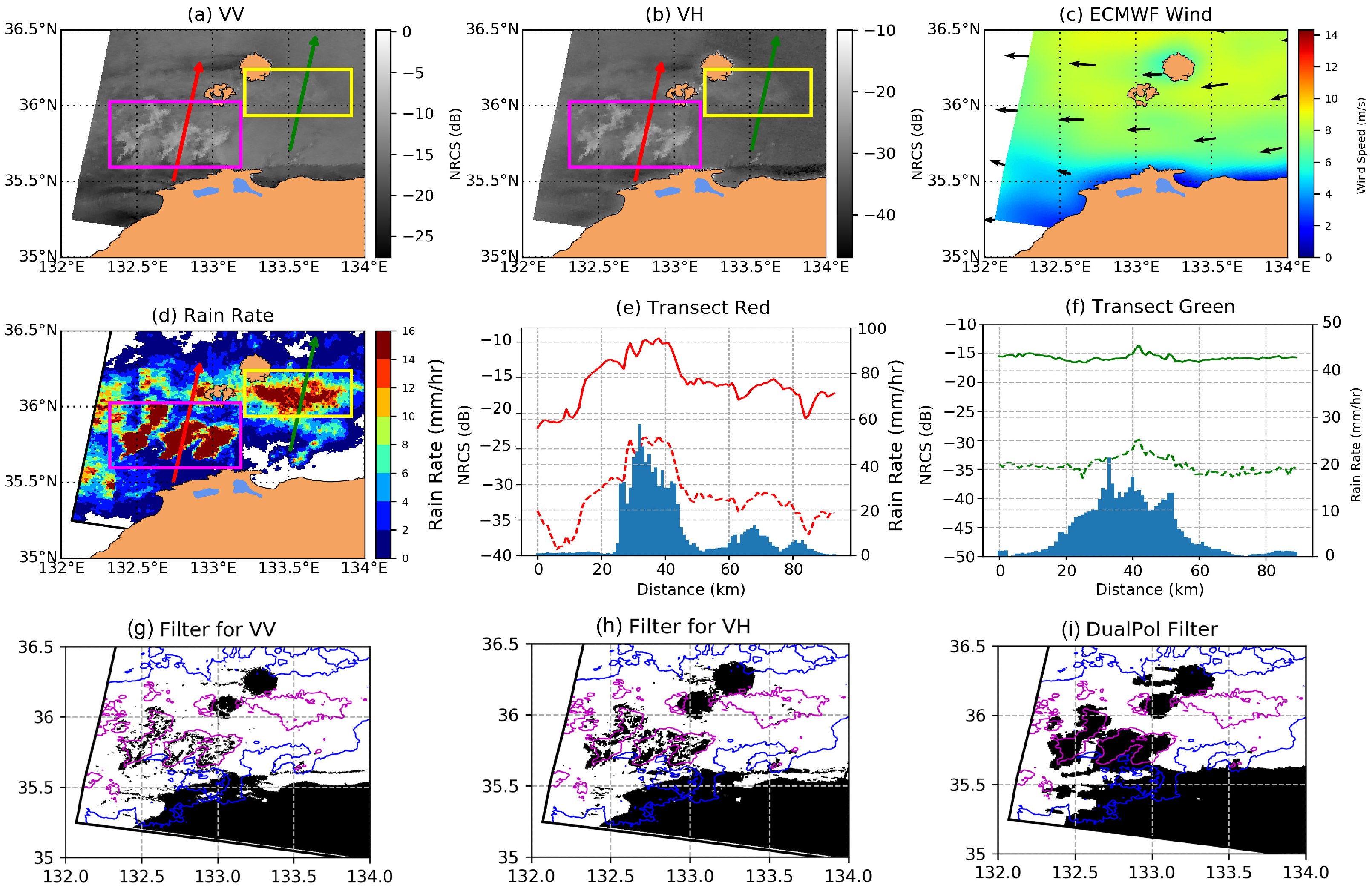
As shown in Figure 10, the detection rate is not 100%, especially for low to medium rain rates and high wind speeds. Indeed, our approach can only detect areas in SAR images where the backscattered signal is significantly affected by rain. Figure 14 illustrates such a case. Here the wind as given by ECMWF is about 9 m/s with two main areas exhibiting rain rates larger than 10 mm/h, but occurring at different incidence angles in the image. The first one (within the purple box) has a stronger rain rate (RR ∈ (14,16) mm/h) and corresponds to larger incidence angles ($\theta \in ({41}^{\circ },{46}^{\circ })$) than the second one (within the yellow box) (RR ∈ (10,14) mm/h; $\theta \in ({38}^{\circ },{41}^{\circ })$). As observed, for the second area, the rain impact on the roughness is much less (see the green transect). Consequently, it is not captured by our detection algorithm. In this case, such a difference between the two signatures probably results from the difference in incidence angle and rain rate.

This case also illustrates that our method does not only detect areas impacted by rain but also by non-wind related features that produce inhomogeneity in the SAR image. Indeed, areas with low backscattered values associated with low winds, such as in the lee of the island (middle) or close to the coast (south part of the area) are detected by our filter. This was already mentioned in the previous study by Koch [25] in which the detection is focused on edges and textural features. As implemented here, the addition of a second channel of polarization as well as the optimization of the detection parameters based on reflectivity measurements from high-resolution radar data is not sufficient for discriminating between various non-wind related phenomena.

5. Conclusions and Perspectives

This study takes benefit of Sentinel-1 C-band SAR mission new capabilities that provides observations over the sea surface in both co- and cross-polarization and of the significant number of data now routinely acquired in coastal areas. Sentinel-1 images have been systematically collocated with high-resolution measurements from ground-based radar from US and Japanese networks.

This unique dataset is used to document the rain impact on C-band co- and cross-polarization backscattered radar signals. We observe that in general, the radar backscattering increases with rain rate for light to moderate winds regime. However, this is not always the case for C-band, since the radar signature of rain can be positive as well as negative, i.e., it can have NRCS values, which are larger or smaller than the NRCS values of the surrounding rain—free area [14,17,40], explaining the variability around the mean trend (see Figure 7). This sensitivity of NRCS to rain rate is found to be more pronounced for higher incidence angles in the case of VV polarization and weak in the case of VH. For the strongest wind conditions analyzed here, the increase is found weaker, yielding to a negative contribution to the radar backscattering for co-polarization. We note that in the case of cross-polarization, the low signal-to-noise ratio observed for low wind speed regimes may have impacted our analysis. Improvements in future mission performance will certainly allow the refinement of this analysis.

The filter as defined by Koch [25] has been implemented on both co- and cross-polarization channels, for different resolutions. A threshold has been defined to maximize the rain detection based on the collocated dataset. We have obtained the result that the combination of the filters computed for each polarization channel at two different resolutions (VV: 400 m and VH: 800 m) improves the rain detection capability in comparison of using only co- or cross-polarization filters. The statistical analysis of NRCS behavior under rain conditions has yielded the result that the detection performance is sensitive to sea-state background, rain rate, and incidence angle. This work also reveals promising results for rain detection in the cases of extreme events such as tropical cyclones.

The dual-polarization filter is hopefully applied on other C-band satellite data, i.e., RADARSAT-2, yet the incidence angle differing from Sentinel-1 might gave slightly different performance. The encouraging performance of a dual-polarization filter to detect rain signatures in SAR images seems to be applicable also to other, non-rain-related features visible on SAR images, such as roll vortices [2]. Additionally, in the particular case of rain detection and segmentation, further work could be done to decipher between the various rain contributions (i.e., stratiform rain, convective rain) and the possible relationship of backscattered signal with lighting events by exploiting the full capability of SAR (for instance, by including phase information), including data from ground–based radars but also other ancillary products such as the Geostationary Global Lightning Mapper (GLM).

References

- Fu, L.L.; Holt, B. Seasat Views Oceans and Sea Ice with Synthetic-Aperture Radar; Jet Propulsion Laboratory, California Institute of Technology: Pasadena, CA, USA, 1982; Volume 81. [Google Scholar]
- Wang, C.; Vandemark, D.; Mouche, A.; Chapron, B.; Li, H.; Foster, R.C. An assessment of marine atmospheric boundary layer roll detection using Sentinel-1 SAR data. Remote Sens. Environ. 2020, 250, 112031. [Google Scholar] [CrossRef]
- Fan, S.; Kudryavtsev, V.; Zhang, B.; Perrie, W.; Chapron, B.; Mouche, A. On C-Band Quad-Polarized Synthetic Aperture Radar Properties of Ocean Surface Currents. Remote Sens. 2019, 11, 2321. [Google Scholar] [CrossRef] [Green Version]
- Kudryavtsev, V.N.; Fan, S.; Zhang, B.; Mouche, A.A.; Chapron, B. On quad-polarized SAR measurements of the ocean surface. IEEE Trans. Geosci. Remote Sens. 2019, 57, 8362–8370. [Google Scholar] [CrossRef]
- Kudryavtsev, V.; Kozlov, I.; Chapron, B.; Johannessen, J. Quad-polarization SAR features of ocean currents. J. Geophys. Res. Ocean. 2014, 119, 6046–6065. [Google Scholar] [CrossRef] [Green Version]
- Horstmann, J.; Wackerman, C.; Falchetti, S.; Maresca, S. Tropical cyclone winds retrieved from synthetic aperture radar. Oceanography 2013, 26, 46–57. [Google Scholar] [CrossRef] [Green Version]
- Zhang, B.; Perrie, W.; Zhang, J.A.; Uhlhorn, E.W.; He, Y. High-resolution hurricane vector winds from C-band dual-polarization SAR observations. J. Atmos. Ocean. Technol. 2014, 31, 272–286. [Google Scholar] [CrossRef]
- Mouche, A.A.; Chapron, B.; Zhang, B.; Husson, R. Combined co-and cross-polarized SAR measurements under extreme wind conditions. IEEE Trans. Geosci. Remote Sens. 2017, 55, 6746–6755. [Google Scholar] [CrossRef]
- Hansen, M.W.; Kudryavtsev, V.; Chapron, B.; Brekke, C.; Johannessen, J.A. Wave breaking in slicks: Impacts on C-band quad-polarized SAR measurements. IEEE J. Sel. Top. Appl. Earth Obs. Remote Sens. 2016, 9, 4929–4940. [Google Scholar] [CrossRef] [Green Version]
- Johansson, A.M.; Brekke, C.; Spreen, G.; King, J.A. X-, C-, and L-band SAR signatures of newly formed sea ice in Arctic leads during winter and spring. Remote Sens. Environ. 2018, 204, 162–180. [Google Scholar] [CrossRef]
- Longépé, N.; Thibaut, P.; Vadaine, R.; Poisson, J.C.; Guillot, A.; Boy, F.; Picot, N.; Borde, F. Comparative evaluation of sea ice lead detection based on SAR imagery and altimeter data. IEEE Trans. Geosci. Remote Sens. 2019, 57, 4050–4061. [Google Scholar] [CrossRef]
- Li, X.M.; Sun, Y.; Zhang, Q. Extraction of Sea Ice Cover by Sentinel-1 SAR Based on Support Vector Machine With Unsupervised Generation of Training Data. IEEE Trans. Geosci. Remote Sens. 2020, 59, 3040–3053. [Google Scholar] [CrossRef]
- Gelis, I.D.; Colin, A.; Longépé, N. Prediction of categorized Sea Ice Concentration from Sentinel-1 SAR images based on a Fully Convolutional Network. IEEE J. Sel. Top. Appl. Earth Obs. Remote Sens. 2021, 14, 5831–5841. [Google Scholar] [CrossRef]
- Melsheimer, C.; Alpers, W.; Gade, M. Investigation of multifrequency/multipolarization radar signatures of rain cells over the ocean using SIR-C/X-SAR data. J. Geophys. Res. Ocean. 1998, 103, 18867–18884. [Google Scholar] [CrossRef]
- Lin, I.I.; Alpers, W.; Khoo, V.; Lim, H.; Lim, T.K.; Kasilingam, D. An ERS-1 synthetic aperture radar image of a tropical squall line compared with weather radar data. IEEE Trans. Geosci. Remote Sens. 2001, 39, 937–945. [Google Scholar] [CrossRef]
- Danklmayer, A.; Doring, B.J.; Schwerdt, M.; Chandra, M. Assessment of Atmospheric Propagation Effects in SAR Images. IEEE Trans. Geosci. Remote Sens. 2009, 47, 3507–3518. [Google Scholar] [CrossRef]
- Alpers, W.; Zhang, B.; Mouche, A.; Zeng, K.; Chan, P.W. Rain footprints on C-band synthetic aperture radar images of the ocean-Revisited. Remote Sens. Environ. 2016, 187, 169–185. [Google Scholar] [CrossRef]
- Braun, N.; Gade, M. Multi-frequency scatterometer measurements on water surfaces agitated by artificial and natural rain. Int. J. Remote Sens. 2006, 27, 27–39. [Google Scholar] [CrossRef]
- Tournadre, J.; Morland, J.C. The effects of rain on TOPEX/Poseidon altimeter data. IEEE Trans. Geosci. Remote Sens. 1997, 35, 1117–1135. [Google Scholar] [CrossRef]
- Olsen, R.; Rogers, D.V.; Hodge, D. The aR b relation in the calculation of rain attenuation. IEEE Trans. Antennas Propag. 1978, 26, 318–329. [Google Scholar] [CrossRef]
- Alpers, W.; Zhao, Y.; Mouche, A.A.; Chan, P.W. A note on radar signatures of hydrometeors in the melting layer as inferred from Sentinel-1 SAR data acquired over the ocean. Remote Sens. Environ. 2020, 253, 112177. [Google Scholar] [CrossRef]
- Lin, W.; Portabella, M.; Stoffelen, A.; Turiel, A.; Verhoef, A. Rain identification in ASCAT winds using singularity analysis. IEEE Geosci. Remote Sens. Lett. 2014, 11, 1519–1523. [Google Scholar] [CrossRef] [Green Version]
- Melsheimer, C.; Alpers, W.; Gade, M. Simultaneous observations of rain cells over the ocean by the synthetic aperture radar aboard the ERS satellites and by surface-based weather radars. J. Geophys. Res. Ocean. 2001, 106, 4665–4677. [Google Scholar] [CrossRef]
- Liu, X.; Zheng, Q.; Liu, R.; Wang, D.; Duncan, J.H.; Huang, S.J. A study of radar backscattering from water surface in response to rainfall. J. Geophys. Res. Ocean. 2016, 121, 1546–1562. [Google Scholar] [CrossRef]
- Koch, W. Directional analysis of SAR images aiming at wind direction. IEEE Trans. Geosci. Remote Sens. 2004, 42, 702–710. [Google Scholar] [CrossRef]
- Longépé, N.; Mouche, A.; Ferro-Famil, L.; Husson, R. Co-Cross Polarization Coherence over the Sea Surface from Sentinel-1 SAR Data: Perspectives for Mission Calibration and Wind Field Retrieval. IEEE Trans. Geosci. Remote Sens. 2021. [Google Scholar] [CrossRef]
- Marshall, J.S.; Palmer, W.M. The distribution of raindrops with size. J. Meteor. 1948, 5, 165–166. [Google Scholar] [CrossRef]
- Atlas, D. Origin of storm footprints on the sea seen by synthetic aperture radar. Science 1994, 266, 1364–1366. [Google Scholar] [CrossRef]
- Moore, R.; Yu, Y.; Fung, A.; Kaneko, D.; Dome, G.; Werp, R. Preliminary study of rain effects on radar scattering from water surfaces. IEEE J. Ocean. Eng. 1979, 4, 31–32. [Google Scholar] [CrossRef]
- Bliven, L.; Sobieski, P.; Craeye, C. Rain generated ring-waves: Measurements and modelling for remote sensing. Int. J. Remote Sens. 1997, 18, 221–228. [Google Scholar] [CrossRef]
- Jameson, A.R.; Li, F.K.; Durden, S.L.; Haddad, Z.S.; Holt, B.; Fogarty, T.; Im, E.; Moore, R.K. SIR-C/X-SAR observations of rain storms. Remote Sens. Environ. 1997, 59, 267–279. [Google Scholar] [CrossRef]
- Katsaros, K.B.; Paris, W.; Vachon, P.G.B.; Dodge, P.P.; Uhlhorn, E.W. Wind fields from SAR: Could they improve our understanding of storm dynamics? Johns Hopkins Apl Tech. Dig. 2000, 21, 86–93. [Google Scholar]
- Browne, I.C.; Robinson, N. Cross-polarization of the radar melting-band. Nature 1952, 170, 1078–1079. [Google Scholar] [CrossRef]
- Jameson, A. The interpretation and meteorological application of radar backscatter amplitude ratios at linear polarizations. J. Atmos. Ocean. Technol. 1989, 6, 908–919. [Google Scholar] [CrossRef] [Green Version]
- Federal Meteorologica Handbook No. 11. In Doppler Radar Meteorological Observations. Part B, Doppler Radar Theory and Meteorology; Technical Report; FCM-H11B-2005; Office of the Federal Coordinator for Meteorological Services and Supporting Research: Washington, DC, USA, 2005.
- Vachon, P.W.; Wolfe, J. C-band cross-polarization wind speed retrieval. IEEE Geosci. Remote Sens. Lett. 2010, 8, 456–459. [Google Scholar] [CrossRef]
- Mouche, A.; Chapron, B. Global C-Band Envisat, RADARSAT-2 and Sentinel-1 SAR measurements in copolarization and cross-polarization. J. Geophys. Res. Ocean. 2015, 120, 7195–7207. [Google Scholar] [CrossRef] [Green Version]
- Tilbury, J.B.; Van Eetvelt, W.; Garibaldi, J.M.; Curnsw, J.; Ifeachor, E.C. Receiver operating characteristic analysis for intelligent medical systems-a new approach for finding confidence intervals. IEEE Trans. Biomed. Eng. 2000, 47, 952–963. [Google Scholar] [CrossRef] [PubMed] [Green Version]
- Youden, W.J. Index for rating diagnostic tests. Cancer 1950, 3, 32–35. [Google Scholar] [CrossRef]
- Atlas, D. Footprints of storms on the sea: A view from spaceborne synthetic aperture radar. J. Geophys. Res. Ocean. 1994, 99, 7961–7969. [Google Scholar] [CrossRef]
Figure 1.
The locations of NEXRAD and JMA coastal stations. (a) The NEXRAD coastal stations over contiguous United States, Hawaii, Guam island and one Japanese island. (b) The locations of JMA radars equipped in the Japanese archipelago.
Figure 2.
Three case studies with SAR data acquired on 13 June 2017 23:20 UTC (Top), 1 September 2017 23:53 UTC (Middle) and 31 August 2017 00:10 UTC (Bottom) with (from Left to Right) Sentinel-1 VV and VH-polarized NRCS images, co-located base reflectivity from NEXRAD at the same time. The wind vectors in the third column refer to ECMWF data. The last column presents the statistics of NRCS with respect to base reflectivity for each case. All these case studies have approximately the same range of incidence angle from about 35 to 41.
Figure 3.
Base reflectivity at different times overlaid on Sentinel-1 VV polarization SAR images. Upper panel: SAR image acquired on 25 June 2017 at 23:21 UTC. The orange contours mark base reflectivities larger than 40 dBZ and the blue contours mark base reflectivities between 20 and −40 dBZ. Lower panel: SAR image acquired on 11 June 2015 at 04:30 UTC. The orange contours mark base reflectivities larger than 35 dBZ and blue contours mark base reflectivities between 20 and −35 dBZ. The overlays (a3,b3) are coincident with the SAR acquisition time.
Figure 4.
The rain rate and NRCS along the transects for the upper case (a) and the lower case (b) in Figure 3. For each case, the upper seven plots with dark curves: Rain rate measured by the weather radar along the transect inserted in the images depicted in Figure 3 at different times. Lower two plots with blue curves: NRCS values measured along the same transect. T0 is the SAR acquisition time.
Figure 5.
Hydrometeor classification at elevation of 0.5 provided by NEXRAD for the three cases in Figure 2.
Figure 6.
Illustration of calculation based on a VV-polarized SAR image. (a) a VV-polarized SAR image acquired on 12 Feb 2017 at 04:29 UTC. The red star marks a single pixel for calculation of . The red rectangle covers the calculation area for the pixel, with a width of 0.5 incidence angle range and the length of 50 km in the azimuth direction. The blue area in the most left panel denotes the calculation area without rain ( dBZ). (b) co-located base reflectivity measured by NEXRAD at the same time and (c) the result of for all the pixels under rain.
Figure 7.
Statistics of with respect to base reflectivity for VV polarization (a-Top) and VH polarization (b-Bottom). The value of rain rate is computed from base reflectivity, according to conversion from NEXRAD manual [35]. The legend in each sub figure stands for the NRCS in rain-free area, suggesting different wind regimes (0–4 m/s, 4–8 m/s, 8–16 m/s, and >16 m/s) as approximately derived with CMOD-5 model. Above histogram denotes the data amount for lines at each base reflectivity bin.
Figure 8.
Illustration of a ROC (True Positive Rate versus False Positive Rate) as Koch filter is applied on VV SAR images at 400 m resolution. The color lines stand for the situation with the different reflectivity ranges.
Figure 9.
Performance of Koch filters at different resolution/polarization with dual-pol filters on the left, and single-pol filter on the right.
Figure 10.
True positive rate of rain detection percentage as a function of rain rate for different wind speed regimes with respect to the polarization channels considered. (a) VV-generated filter, (b) VH-generated filter and (c) dual-pol filter.
Figure 11.
True positive rate of rain detection percentage as function of incidence angle for the polarization channels considered with respect to different rain rates. The first bin at 32 is affected by artefacts linked to recurrent invalid data at near range.
Figure 12.
The first and second columns show the Koch filters generated with VV (400 m) and VH (800 m) channels respectively for the three cases in Figure 2. The last column shows the proposed dual-pol filters correspondingly. The blue and purple contours mark the base reflectivity of 20 dBZ and 40 dBZ respectively.
Figure 13.
(a,b) are VV- and VH-pol Sentinel-1 SAR images acquired over the Gulf of Mexico on 10 September 2017 at 23:27 UTC showing radar signatures of rain bands associated with the tropical cyclone IRMA. (c) base reflectivity from the NEXRAD KAMX station. (d,e) the masks generated only by single-pol VV/VH. (f) the dual-pol filter. The blue and purple contours in (d–f) mark the base reflectivity of 20 dBZ and 40 dBZ respectively.
Figure 14.
(a,b) show the S-1 maps at VV and VH at 21:08 UTC on 3 September 2019. (c) shows wind speed and direction from ECMWF. Rain rate provided by JMA are displayed on (d). (e) the masks generated only by single-pol VV/VH and by our proposed algorithm. (f) shows NRCS along two transects inserted in SAR images. Two rectangles are overlaid on (a,b,d) to demonstrate the 2 area with heavy rain. (g,h) the masks generated only by single-pol VV/VH. (i) the dual-pol filter.
Publisher’s Note: MDPI stays neutral with regard to jurisdictional claims in published maps and institutional affiliations. |
© 2021 by the authors. Licensee MDPI, Basel, Switzerland. This article is an open access article distributed under the terms and conditions of the Creative Commons Attribution (CC BY) license (https://creativecommons.org/licenses/by/4.0/).
Share and Cite
MDPI and ACS Style
Zhao, Y.; Longépé, N.; Mouche, A.; Husson, R. Automated Rain Detection by Dual-Polarization Sentinel-1 Data. Remote Sens. 2021, 13, 3155. https://0-doi-org.brum.beds.ac.uk/10.3390/rs13163155
AMA Style
Zhao Y, Longépé N, Mouche A, Husson R. Automated Rain Detection by Dual-Polarization Sentinel-1 Data. Remote Sensing. 2021; 13(16):3155. https://0-doi-org.brum.beds.ac.uk/10.3390/rs13163155
Chicago/Turabian StyleZhao, Yuan, Nicolas Longépé, Alexis Mouche, and Romain Husson. 2021. "Automated Rain Detection by Dual-Polarization Sentinel-1 Data" Remote Sensing 13, no. 16: 3155. https://0-doi-org.brum.beds.ac.uk/10.3390/rs13163155
Note that from the first issue of 2016, this journal uses article numbers instead of page numbers. See further details here.