Article

Deep Learning for Polarimetric Radar Quantitative Precipitation Estimation during Landfalling Typhoons in South China

1
School of Geographical Sciences, Nanjing University of Information Science & Technology, Nanjing 210044, China
2
Guangdong Meteorological Public Service Center, Guangzhou 510641, China
3
Institute of Artificial Intelligence for Meteorology, Chinese Academy of Meteorological Sciences, Beijing 100081, China
4
State Key Laboratory of Severe Weather, Chinese Academy of Meteorological Sciences, Beijing 100081, China
5
Department of Electrical and Computer Engineering, Colorado State University, Fort Collins, CO 80523, USA
6
Guangdong Emergency Early Warning Release Center, Guangzhou 510641, China
7
Guangdong Technology Support Center of Flood Control, Guangzhou 510635, China
*
Author to whom correspondence should be addressed.
Remote Sens. 2021, 13(16), 3157; https://0-doi-org.brum.beds.ac.uk/10.3390/rs13163157
Submission received: 20 July 2021 / Revised: 6 August 2021 / Accepted: 7 August 2021 / Published: 10 August 2021

Abstract

:
Heavy rain associated with landfalling typhoons often leads to disasters in South China, which can be reduced by improving the accuracy of radar quantitative precipitation estimation (QPE). At present, raindrop size distribution (DSD)-based nonlinear fitting (QPEDSD) and traditional neural networks are the main radar QPE algorithms. The former is not sufficient to represent the spatiotemporal variability of DSDs through the generalized Z–R or polarimetric radar rainfall relations that are established using statistical methods since such parametric methods do not consider the spatial distribution of radar observables, and the latter is limited by the number of network layers and availability of data for training the model. In this paper, we propose an alternative approach to dual-polarization radar QPE based on deep learning (QPENet). Three datasets of “dual-polarization radar observations—surface rainfall (DPO—SR)” were constructed using radar observations and corresponding measurements from automatic weather stations (AWS) and used for QPENetV1, QPENetV2, and QPENetV3. In particular, 13 × 13, 25 × 25, and 41 × 41 radar range bins surrounding each AWS location were used in constructing the datasets for QPENetV1, QPENetV2, and QPENetV3, respectively. For training the QPENet models, the radar data and AWS measurements from eleven landfalling typhoons in South China during 2017–2019 were used. For demonstration, an independent typhoon event was randomly selected (i.e., Merbok) to implement the three trained models to produce rainfall estimates. The evaluation results and comparison with traditional QPEDSD algorithms show that the QPENet model has a better performance than the traditional parametric relations. Only when the hourly rainfall intensity is less than 5 mm (R < 5 mm·h−1), the QPEDSD model shows a comparable performance to QPENet. Comparing the three versions of the QPENet model, QPENetV2 has the best overall performance. Only when the hourly rainfall intensity is less than 5 mm (R < 5 mm·h−1), QPENetV3 performs the best.

1. Introduction

Heavy rain from landfalling typhoons is one of the major natural disasters in South China, which often causes life and economic losses [1]. High-resolution precipitation estimation is a prerequisite for the typhoon rainfall forecast. The polarimetric radar (PR) is an efficient tool for observing precipitation and its microphysical structures [2]. The PR has significant advantages in quantitative precipitation estimation (QPE) over the single-polarization radar due to enhanced observations of the precipitation particle size, shape, and orientation [3].
QPE algorithms have been studied for many years using the PR measurements. In principle, the quantitative relation between the surface rainfall and radar observation aloft can be obtained from measurements [3]. However, it is difficult to present this functional relation in a simple form due to the complex spatiotemporal variability in DSDs [4,5], especially during typhoon events which are often characterized by complicated precipitation microphysical processes [6]. At present, DSD-based nonlinear fitting algorithms (hereafter referred to as the QPEDSD method) [2,5,7] and the traditional neural network approach [8,9,10,11] are the main QPE algorithms. The precipitation estimation accuracy of the parametric QPEDSD methods is determined by the physical model of DSD and the relationship between the physical model and the radar parameters [2,12,13]. DSD characteristics vary with the location and precipitation type. The parameter relationships between rain rate (R) and the polarimetric radar observables, including reflectivity (ZH), differential reflectivity (ZDR), and the specific differential phase (KDP), are not sufficient to characterize the variation [14,15,16,17]. In addition, the traditional neural network method is limited by the number of network layers and the availability of training data, resulting in poor learning performance.
In recent years, deep learning has been widely used in the fields of computer vision [18,19] and geoscience including precipitation research (e.g., [20,21]). Tan et al. built a deep neural network to estimate precipitation based on radar and surface rainfall observation data [22,23]. Chen et al. proposed a neural network based on a fusion mechanism to improve satellite precipitation retrievals using ground radar estimates [24]. Chandrasekar et al. [25] and Chen et al. [3] constructed a precipitation estimation algorithm composed of two deep neural networks in order to establish the relationship between a spaceborne radar and rain gauges using a ground radar as a bridge. Moraux et al. proposed a deep-learning precipitation estimation method based on satellite and rain gauge observations [26]. The abovementioned studies show that deep-learning algorithms have great potential for improving radar-based QPE.
In this study, we extended the deep learning applications for radar QPE in south China, with an emphasis on typhoon events. This study used hybrid volume scan data of ZH, ZDR, and KDP for precipitation estimation, which can better represent the actual cloud and rainfall conditions and help reduce systematic biases. In particular, a deep convolutional neural network (CNN) composed of multiscale convolutional operations was designed to realize the complex nonlinear mapping from radar measurements to rainfall rate. This multiscale encoding–decoding network structure had strong feature extraction and fitting capability, as well as the invariance of displacement, scale, and deformation. It could better extract the spatial characteristics of precipitation from radar data and learn the relationship between multidimensional radar observations and surface rainfall. In addition, for the same CNN structure, we used three different datasets to quantify the areal representation of radar observables and address which range bins should be used to obtain reliable precipitation estimates. In particular, 13 × 13, 25 × 25, and 41 × 41 radar range bins surrounding each AWS location were used in constructing the three datasets. For training the QPENet models, the radar data and AWS measurements from eleven landfalling typhoons in South China during 2017–2019 were used. For demonstration, an independent typhoon event was randomly selected (i.e., Merbok) to evaluate the trained models and compare with the traditional QPEDSD algorithms.
The remainder of this paper is organized as follows. Section 2 introduces the datasets used in this study. Section 3 details the deep learning-based radar QPE methodology, including the model architecture and training strategy, as well as how to construct the model input data for machine learning. In Section 4, the precipitation estimation accuracy of the three trained models is evaluated, and the influence of the input data dimension on the model results is thoroughly discussed. Section 5 compares the data with the conventional radar QPE algorithm while Section 6 summarizes the main findings of this research.

2. Data

Eleven heavy rainfall events caused by landfalling typhoons in South China from 2017 to 2019 were used in this study. Figure 1 shows the tracks of the eleven typhoons and the locations of the Guangzhou radar and nearby surface automatic weather stations (AWS). Table 1 lists the detailed information of these eleven typhoon events.

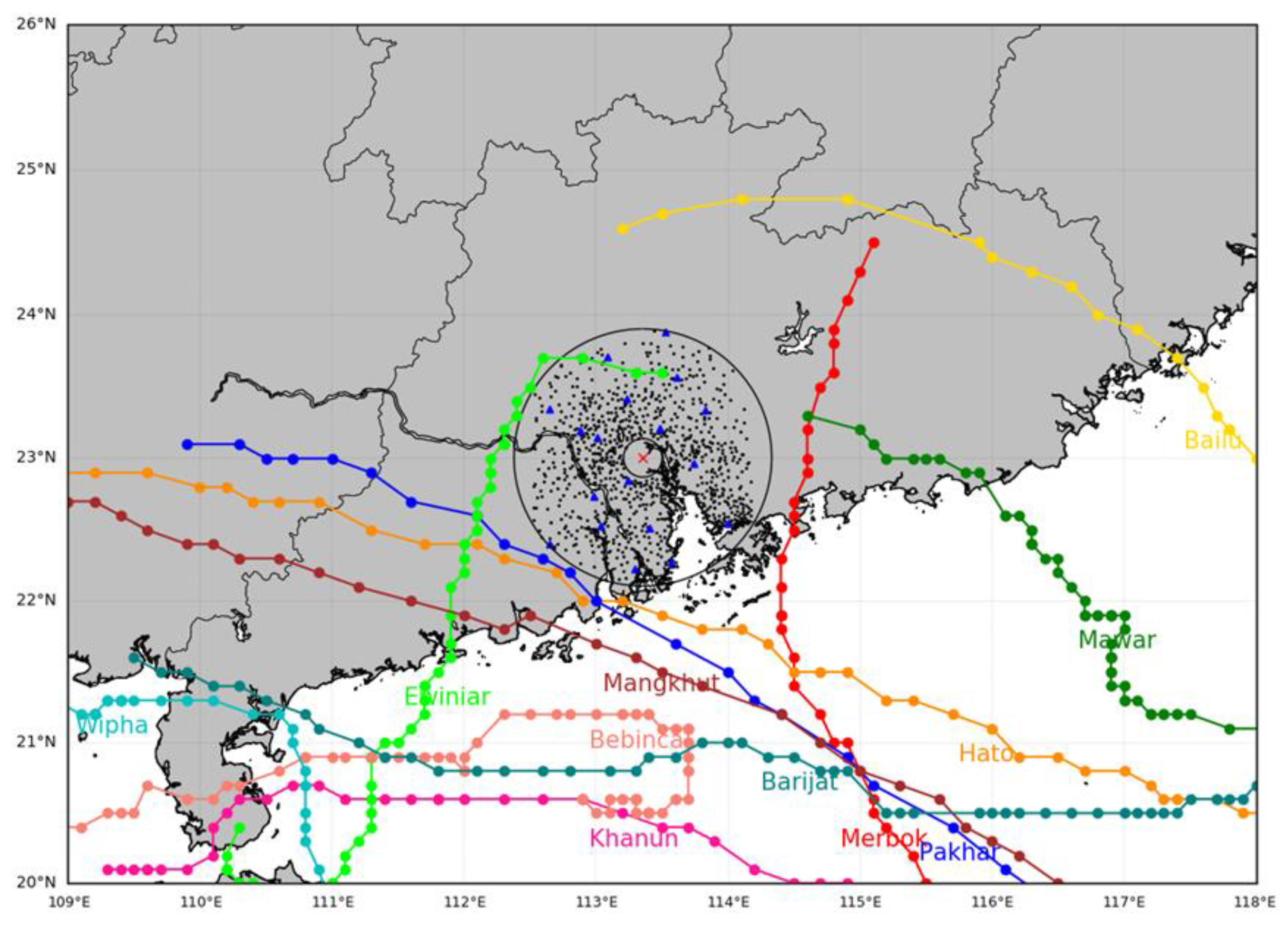
2.1. Dual-Polarization Radar Data

In 2016, the Guangzhou radar was upgraded with dual-polarization capability. According to the standards of the China Meteorological Administration (CMA), this radar has been calibrated by the manufacturer [27]. After the dual-polarization upgrade, the Meteorological Observation Center of the CMA conducted a series of tests, such as the built-in system component test and routine calibrations. The test results show that the measurement uncertainty of ZH is less than 1 dB, and the measurement uncertainty of ZDR is less than 0.4 dB. The radar operates with the general volume coverage pattern 21, which scans every six minutes with nine elevation angles (0.5°, 1.5°, 2.4°, 3.3°, 4.3°, 6.0°, 9.9°, 14.6°, and 19.5°). The radar beamwidth is 0.95°, the radial resolution is 0.25 km, and the commonly used maximum detection distance is 230 km.
In this study, polarimetric radar data in the range of 15–100 km from the radar (see Figure 1) were used in order to reduce the influence of the zero-degree layer and the interference of near-range ground objects. The selected eleven typhoon events consisted of 3150 volume scans, and the numbers of scans for each typhoon event are detailed in Table 1. In addition, thorough quality control was performed on the collected radar data, including removal of outliers and non-meteorological echoes, differential phase ΦDP processing, KDP estimation, etc. [28]. The quality-controlled data were used as the input to the deep-learning model for precipitation estimation.

2.2. Automatic Weather Station (AWS) Data
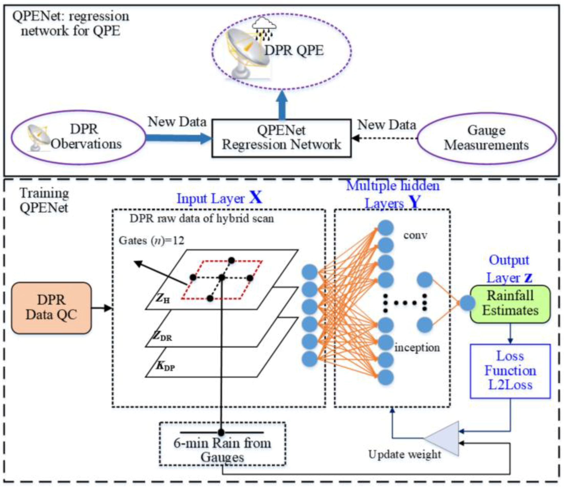
In this study, the rainfall observations from 18 national and 1041 regional automatic weather stations were used as target labels in training the deep-learning model. The locations of the AWS relative to the Guangzhou radar are indicated in Figure 1. The AWS rainfall resolution is 0.1 mm, and the rainfall data is archived every five minutes, including one-minute rainfall and five-minute accumulated rainfall. The six-minute accumulated rainfall can be obtained through the one-minute rainfall observation in order to match the radar observation times. Here, it should be noted that the method of Gou et al. [29] was used to control the quality of rainfall observations from the AWS and remove the suspicious records.

3. Methods

To test our deep-learning QPE method, the dataset was divided into two independent parts: the training dataset and the test dataset. The former was used to train the model by optimizing the learnable parameters of the model through the back-propagation algorithm [21]. In order to ensure that our model did not overfit the training data and could at the same time make full use of the existing data, we used the k-fold cross-validation method to optimize the network structure and training strategy through the performance evaluation of the k-fold validation dataset. The model and training strategy that performed the best on the validation dataset may overfit the dataset. Therefore, an independent test dataset was required for the final evaluation of the model.
In the following section, we describe in more detail how the data were prepared before being fed to our model, how the dataset was made for the training model, and how we split the data into the training dataset and the test dataset. Furthermore, we present the architecture of our model and its training strategy.

3.1. Model Inputs

The input features of the QPENet model are the dual-polarization radar-based data, and the target labels are rainfall measurements from the surface automatic weather stations. The QPENet model needs to be trained by datasets with tags. The model inputs used by Chen et al., the CAPPI reflectivity profiles with the horizontal resolution of 1 km and heights of 1, 2, 3, and 4 km, were not used in our model [3]. To preserve the original radar information in the network and include the polarization quantities closely related to precipitation microphysics, this study proposed using multiple polarimetric observables from the hybrid scan strategy as the inputs. In order to construct the dataset, we should have first found the corresponding relationship between the dual-polarization radar data and surface rainfall. Properly connecting the surface rainfall values (target labels) with multidimensional radar measurements was critical to training the machine-learning model for enhanced precipitation estimates.
In particular, at a given time and AWS location, we built the matching samples between rainfall measurements from the AWS and polarimetric variables at the elevation angles and different ranges surrounding the AWS. A trustworthy data sample (Figure 2) was obtained through adjusting the radar observation range (range bins surrounding the AWS), observation height (elevation angles), and polarization quantity (ZH, ZDR, and KDP).
The specific steps for establishing the data sample and dataset of “DPO—SR” are as follows (Figure 2):
(1) Automatic weather station selection: To avoid the influence of the melting layer and ground clutter, only the automatic weather stations within 15–100 km of the radar with rainfall greater than 0.1 mm were used in this study.
(2) Hybrid scan: It is formed by the four lowest elevation angles. To avoid the effect of ground clutter, the fourth elevation angle (3.3°) was selected for 15–20 km away from the radar, the third elevation angle (2.4°) was selected for 20–35 km, the second elevation angle (1.5°) was selected for 35–50 km, and the first elevation angle (0.5°) was selected for 50–100 km.
(3) Location correspondence: According to the distance from the automatic weather station to the radar, the range bin closest to the station at the corresponding elevation angle was selected as the corresponding range bin.
(4) Range bin selection: The range bin matrix of (2n + 1) × (2n + 1) was composed of the front and back n range bins in the same radial direction of the corresponding range bin and the right and left n radial directions of the corresponding range bins at the selected elevation angle.
(5) Generation of data samples: The matrix composed of the polarization quantities within the radar observation range bin (called data) and the observed rainfall amount (called label) from the corresponding automatic weather station was generated as a sample.
(6) Steps (1)–(5) are the process of labeling (tagging) the rainfall from automatic weather stations for dual-polarization radar observations. The “dual-polarization radar observation—surface rainfall” dataset was generated by repeating the tagging process.
Generally, the wind is stronger in typhoon precipitation. Affected by the wind, the range of falling raindrops is relatively wide. In other words, a wider range of radar observations is related to the rainfall observed by surface automatic stations. In order to obtain a better correspondence between the dual-polarization radar observations and surface rainfall, a sample and the dataset of “DPO—SR” were established, which are more conducive to precipitation estimation; 13 × 13, 25 × 25, and 41 × 41 bins surrounding the range bin on top of the AWS were chosen as the radar observation range bins, that is, the radar observation areas roughly at 1.5 km, 3 km, and 5 km away from the surface automatic weather stations were selected to correspond to the surface rainfall, and the QPE datasets (see Table 2 for details) for version 1 (13 × 13), version 2 (25 × 25), and version 3 (41 × 41) of the eleven typhoon events were respectively established to analyze the influence of the radar observation range on the typhoon precipitation estimation.

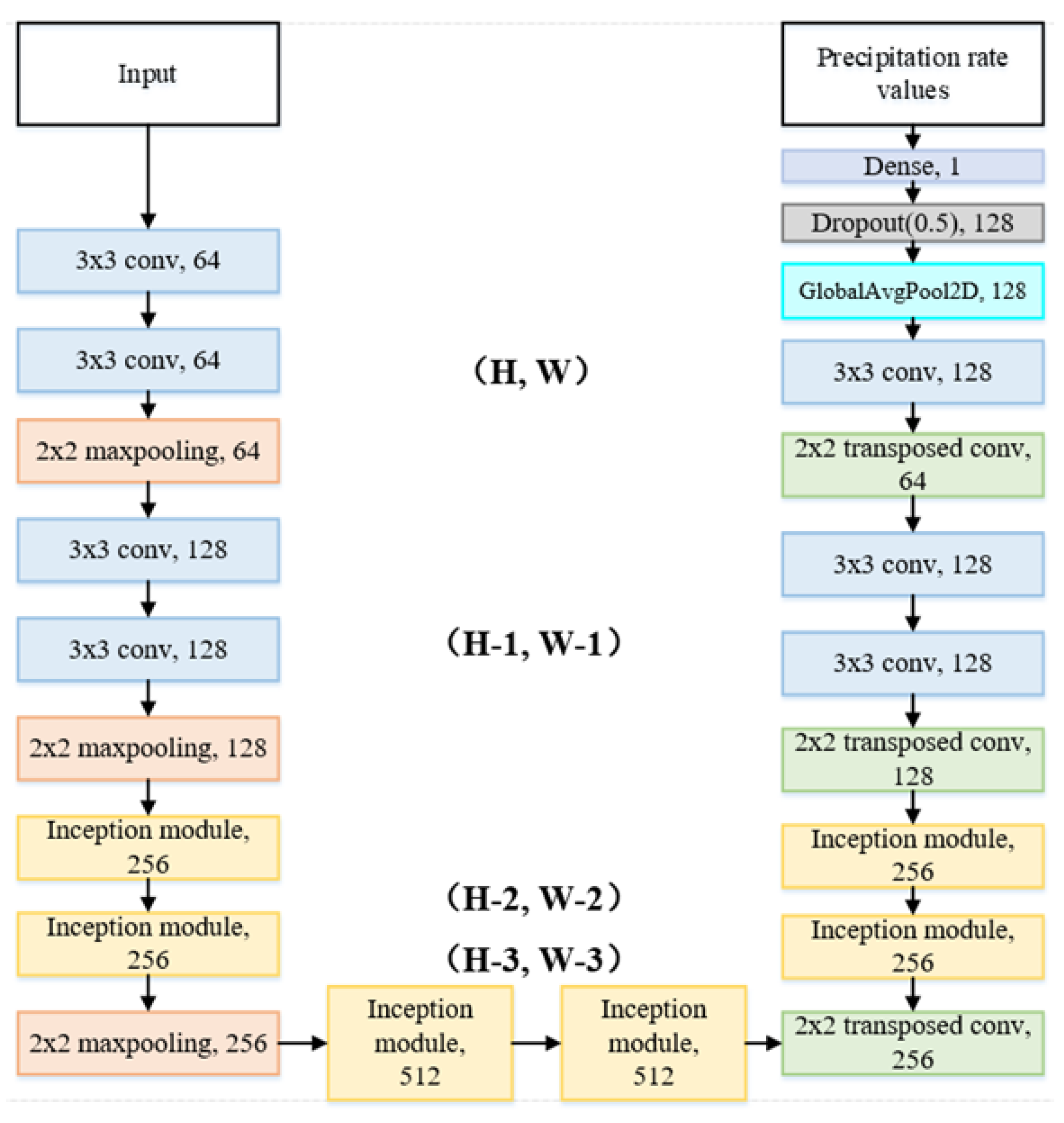
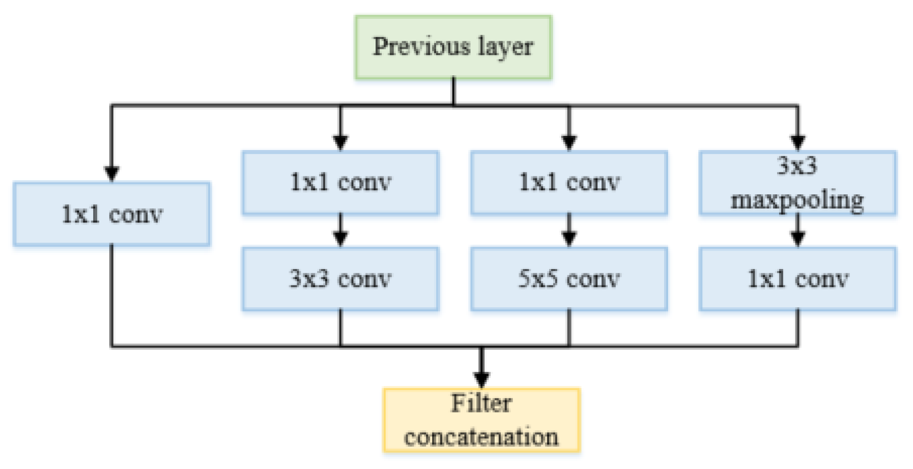
3.2. Model Architecture

The invariance of CNN displacement, scale, and deformation was used to extract the spatial features of radar data to better fit the relationship between radar observations and surface rainfall and give full play to the excellent feature extraction and fitting performance of the deep neural network (DNN). QPENet training and estimation processes (Figure 3) were designed to estimate the precipitation based on the classic DNN and CNN architectures, modules, and concepts (such as AlexNet [30], GoogLeNet [31], and ResNet [32]). The QPENet model is a regression deep CNN architecture directly facing the automatic weather station rainfall. It takes radar observation data as the inputs, automatic weather station rainfall as the target data, and mean square error as the loss function. The features in the inception module were used to extract multiscale precipitation features through multiple convolution kernels with different sizes. In particular, radar observations and the corresponding surface automatic weather station precipitation were used to train the QPENet regression network (the lower panel in Figure 3). The trained model could estimate surface precipitation based on the new radar observations (the upper panel in Figure 3) and evaluate its estimation accuracy through rainfall observation at new automatic weather stations.
The general expression of the QPENet model is as follows [3].
y 1 = f ( w 1 X + b 1 )
y n = f ( w n y n 1 + b n )
      Z = f ( w n + 1 y n + b n + 1 )
where X is the input variable which refers to multiple polarization parameters (i.e., ZH, ZDR, and KDP) of the radar at different ranges (i.e., 1.5 km, 3 km, and 5 km.); y 1 y n are the outputs of the hidden layers; w 1 is the weight vector for the input data; w 2 w n + 1 are the weights of the n hidden layers; b 1 b n + 1 are the biases associated with the input layers and the hidden layers; Z is the output (i.e., precipitation estimation) compared with the target labels (i.e., AWS-measured rainfall) to update the weights.
Our problem was very similar to the semantic segmentation application, and the purpose of the latter is to assign each pixel in the image to a category. For example, the hourglass-shaped network (HSN) is a kind of a convolutional neural network which can analyze the multiscale input, showing a good performance in the semantic segmentation of aerial images [33]. Due to the abovementioned reasons, our model could be divided into two parts, the encoder and the decoder (Figure 4). The encoder gradually reduced the input resolution through its maximum pooling layer, allowing the convolution kernel of the next layer to cover a larger spatial range. In addition, we used inception layers to further improve the multiscale conversion capability of the model [31] (Figure 5 and Table 3). These layers were composed of convolutional layers with different convolution kernel sizes to perform conversions of different scales. The decoder followed a pattern similar to the encoder. After the third maximum pooling layer, the transposed convolution was used instead of the maximum pooling layer to increase the resolution gradually. In this way, our model recovered the details lost in the continuous maximum pooling layer, reaching the highest resolution at the input time. Finally, the rain rate (R; units: mm·h−1) was obtained through the GlobalAvgPool2D, Dropout, and Dense layers at the end of the decoder.

3.3. Training Strategies

To train the model, we randomly chose one of the eleven typhoon precipitation events as the test dataset and the remaining ten as the training (validation) dataset. The k-fold cross-validation method randomly selected nine of the ten typhoons as the training dataset and one as the validation dataset. After ten training sessions, the hyperparameter tuning of the network based on the network performance of the verification dataset was determined. To prevent the model from overfitting, the test dataset was used to evaluate its generalization ability.
To explore the influence of the radar observation range on the precipitation estimation, three versions (V1, V2, and V3) of the QPE dataset were used to train the model. The numerical stability of deep-learning model training is related to the quality of the training results [31]. In order to ensure the numerical stability of the training process and obtain better training results, we normalized the input data (radar observation) and target data (automatic weather station precipitation) so that their mean value was 0, variance was 1, and their values were between 0 and 1.
Finally, based on the deep learning library of MXNet/Gluon from Amazon, the model selected Xavier for parameter initialization [34]. The Adam optimization algorithm with a learning rate of 10−3 and the method of early stopping were adopted, and four Nvidia Tesla P100s were used for training. The specific hyperparameter, the convergence epochs of our model, and the time spent on each batch are shown in Table 4.

3.4. Evaluation Method

Based on the test dataset, the automatic weather station rainfall was taken as the reference, and then the 6-min radar data was input into the network. By accumulating the output, the hourly rainfall intensity could be obtained. Furthermore, five indicators of correlation coefficient (CC), root-mean-square error (RMSE), normalized relative bias (NB), normalized absolute error (NE), and bias ratio were used to evaluate the estimation accuracy comprehensively. The results were then compared with the results of the QPEDSD method.
CC = i = 1 n ( RA i radar RA i radar ¯ ) ( RA i gauge RA i gauge ¯ ) i = 1 n ( RA i radar RA i radar ¯ ) 2 i = 1 n ( RA i gauge RA i gauge ¯ ) 2
RMSE = i = 1 n ( RA i radar RA i gauge ) 2 n
NB = i = 1 n ( RA i radar RA i gauge ) i = 1 n R i DSD × 100
NE = i = 1 n | RA i radar RA i gauge | i = 1 n RA i gauge × 100
bias   ratio = i = 1 n RA i radar i = 1 n RA i gauge
In the equations above, RA is the one-hour accumulated rainfall from the radar or automatic stations, and the overline indicates the average value; n is the number of RAigauge–RAiradar pairs; the units of measurement of the RMSE are millimeters; NE and NB are both percentages; and the bias ratio greater (or less) than 1 indicates overestimation (or underestimation).

4. Results

In this section, one typhoon from the eleven typhoon events in South China in 2017–2019 was randomly chosen to examine the QPENet algorithm for the operational Guangzhou radar. The Merbok (1702) typhoon event was taken as an example, and the QPEDSD and QPENetV2 algorithms were used to estimate the hourly average rainfall intensity (Figure 6) and accumulated rainfall intensity of this event. Figure 6 and Figure 7 show that the spatial distributions of hourly average rainfall intensity and accumulated rainfall intensity of these two estimation algorithms were basically the same, both consistent with actual precipitation events.

4.1. Performance of the QPENet Algorithm

Table 1 shows the eleven typhoon events that occurred in South China. The evaluated scores on four kinds of QPE algorithms for all rainfall intensities for the Merbok (1702) event are shown in Table 5, the scores for the rainfall intensity less than 5 mm·h−1 are shown in Table 6, the scores for the rainfall intensity greater than or equal to 5 mm·h−1 and less than 30 mm·h−1 are shown in Table 7, and the scores for the rainfall intensity greater than or equal to 30 mm are shown in Table 8. The four kinds of QPE algorithms are QPENetV1, QPENetV2, QPENetV3, and QPEDSD [35,36]. QPENetVn refers to the QPENet deep-learning model trained with the dataset of version n (n = 1, 2, or 3). QPEDSD refers to the QPE algorithm based on DSD fitting.
From Table 5, Table 6 and Table 7, it is found that the QPENet algorithms had better estimation performance than the QPEDSD algorithm, whether for the process with 5 ≤ R < 30 and R ≥ 30 mm·h−1 or for all the rainfall intensities. Only when R < 5 mm·h−1, the underestimation of the QPEDSD algorithm was small, and the overestimation of the QPENet algorithm was large. However, the RMSE of QPENet was small and the algorithm was relatively stable. Considering that weak precipitation has a small impact on daily life, these two algorithms are both applicable.
The evaluation indicators of the QPENet and QPEDSD algorithms were analyzed as follows. For all the rainfall intensities, the CC, RMSE, NB, NE, and bias ratio were increased by 0.2%, 39%, 73%, 17%, and 73% at the most, respectively. When R was greater than or equal to 5 mm·h−1 and less than 30 mm·h−1, the CC, RMSE, NB, NE, and bias ratio could be increased by −1%, 32%, 96%, 31%, and 96% at the most, respectively. When R was greater than or equal to 30 mm·h−1, the CC, RMSE, NB, NE, and bias ratio were increased by 4%, 47%, 34%, 34%, and 34% at the most, respectively. For the three situations of rainfall intensity above, the QPENet algorithms had apparent advantages. However, when R was less than 5 mm·h−1, the CC, RMSE, NB and bias ratio were increased by 19%, 28%, 6%, and −37% at the most, respectively. The performance of the QPEDSD algorithm was slightly better, indicating that the QPENet algorithm still has room for improvement when there is weak precipitation.

4.2. Effect of Input Data on the Performance of the QPENet Algorithms

During the rainfall episode of landfall typhoons, the wind is relatively strong. When establishing the corresponding relationship between dual-polarization quantities and surface automatic weather station observations, the influence of wind needs to be considered. Therefore, according to the distance from the surface automatic weather stations, this study established three versions of the QPE dataset: version 1 was 1.5 km away from the surface rainfall observation station, version 2 was 3 km away from the rainfall station, and version 3 was 5 km away from the rainfall station. After the QPENet model training for the three versions of the dataset, three precipitation estimation models of QPENetV1, QPENetV2, and QPENetV3 were obtained. According to Table 5, Table 6, Table 7 and Table 8, QPENetV2 had the best comprehensive estimation performance on all the rainfall intensities, 5 ≤ R < 30 mm·h−1 and R ≥ 30 mm·h−1. It shows that radar observations 3 km away from the stations were the most relevant to surface precipitation observations in the three cases above. When hourly rainfall intensity was less than 5 mm, QPENetV3 had the best estimation performance out of the three deep-learning algorithms. This may have been because the position of light rain falling to the surface is uncertain, and lighter rain has smaller drops that are advected further between the height of the radar beam and the surface.

5. Performance Comparisons between the QPEDSD and QPENetV2 Algorithms

According to the analysis in Section 4, the QPENetV2 algorithm had the best comprehensive performance among the three trained deep-learning models. This section compares the performance of QPENetV2 and the traditional QPEDSD method in detail in three aspects.

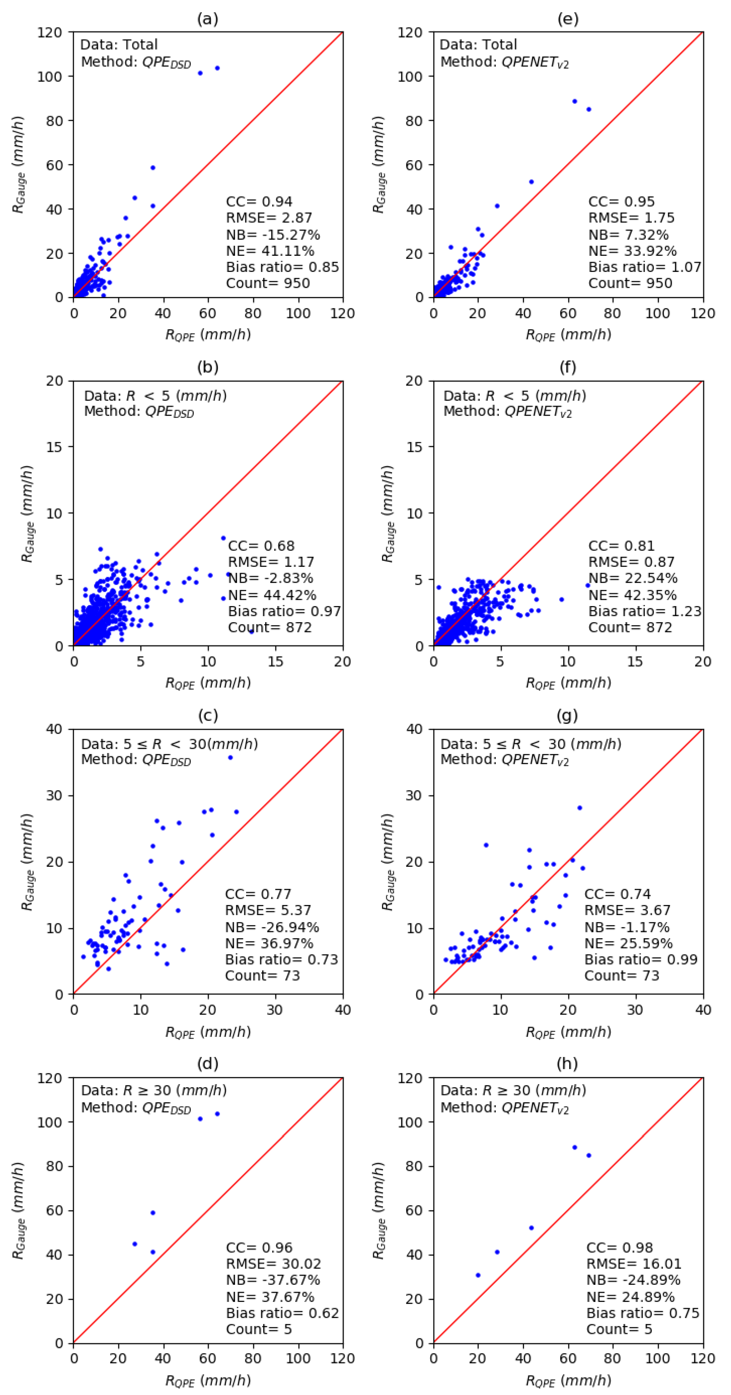
5.1. Performance of QPEDSD and QPENetV2 under Different Rainfall Intensities

The scatterplots of the radar rainfall estimates from QPEDSD and QPENetV2 versus AWS measurements under different rainfall intensities are shown in Figure 8. When R < 5 mm·h−1, the estimation accuracy of QPEDSD was slightly better than that of QPENetV2. It may have been due to the relatively large measurement uncertainty of the polarimetric radar variables (ZDR and KDP) during light rain. Since the QPEDSD algorithm was based on the segmentation of rain intensity, which takes into account the distribution of light rain, it showed a slightly better performance. However, for all the other rainfall intensities, the QPENetV2 algorithm had obvious advantages.

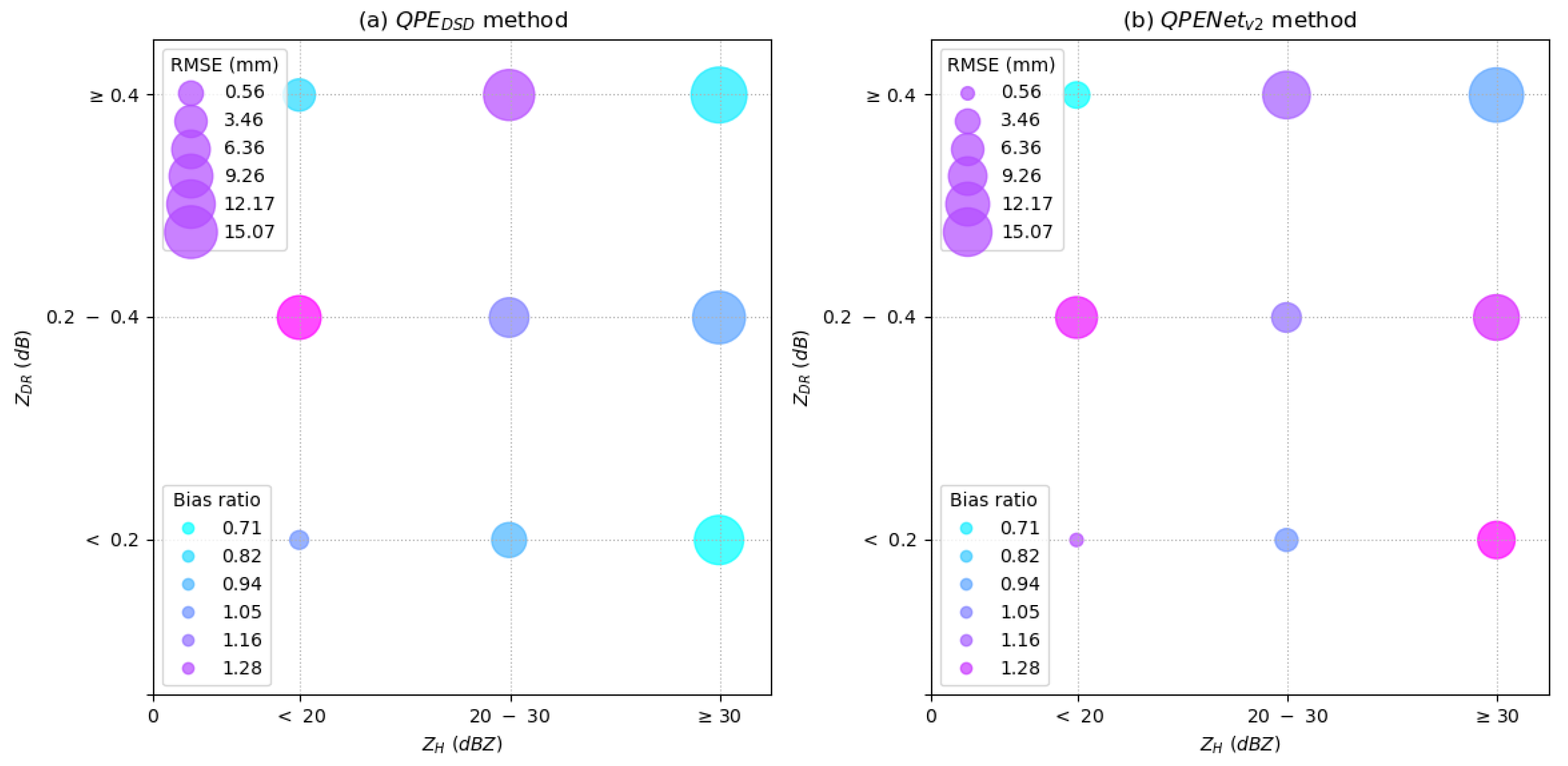
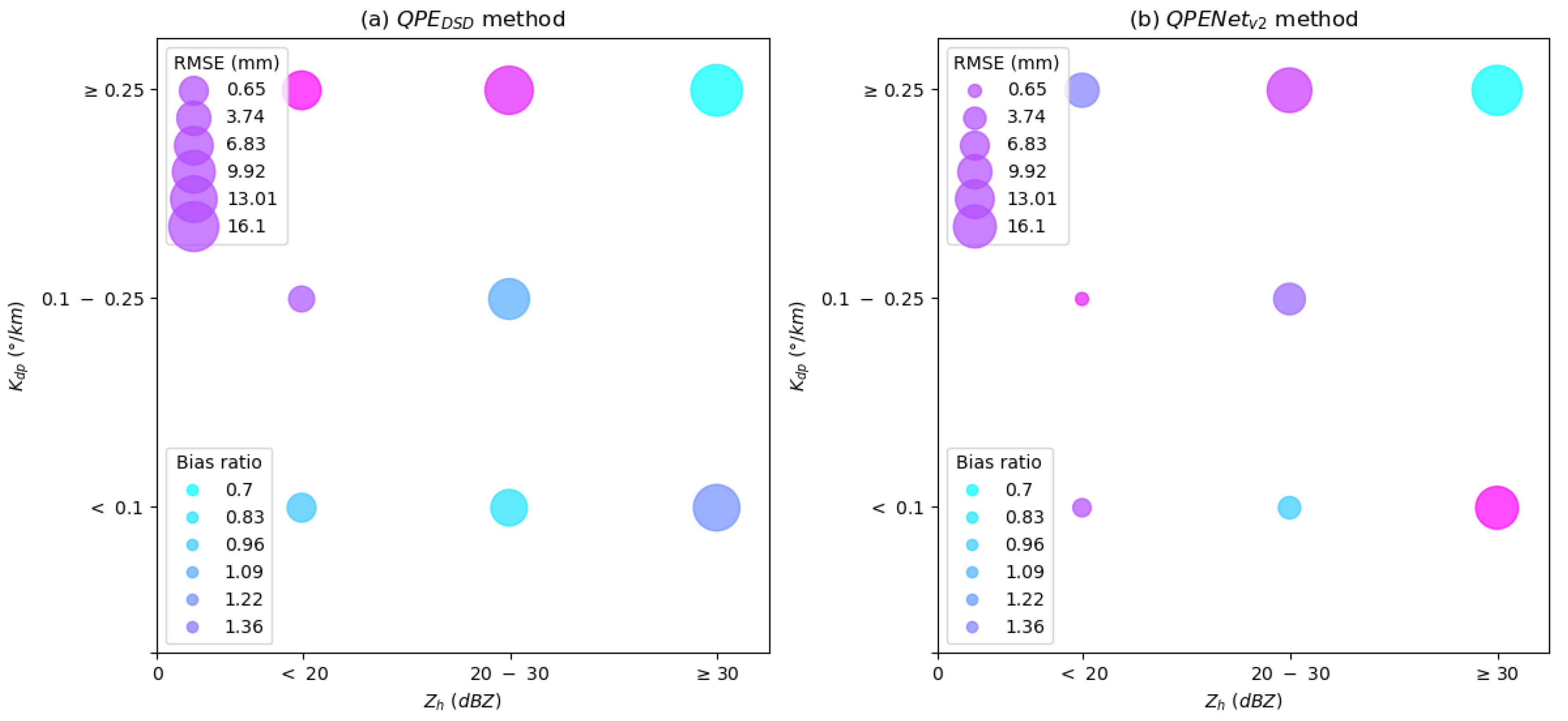
5.2. Performance of QPEDSD and QPENetV2 on Different Segments of ZH, ZDR, and KDP

The bias ratio and RMSE of the derived rainfall estimates using the QPEDSD and QPENetV2 algorithms were compared for different segments of ZH and ZDR (Figure 9). When ZH was small (<20 dBZ), the bias ratios of the two algorithms first increased and then decreased as ZDR increased, and the bias ratio of QPENetV2 decreased faster. When ZH was moderate (20–30 dBZ), the bias ratios increased with ZDR, and the bias ratio of QPENetV2 increased slower. When ZH was large (≥30 dBZ), the bias ratio of QPEDSD first increased and then decreased with the increase in ZDR, while the bias ratio of QPENetV2 decreased with the increase in ZDR.
Overall, the RMSE of QPENetV2 was smaller than that of QPEDSD, indicating that the former was more stable. But the RMSEs of both algorithms in the upper right corner were rather large, which means when ZH and ZDR are large, the stability of both algorithms has room for improvement.
On specific segments of ZH and KDP, the bias ratio and RMSE of precipitation estimates from QPEDSD and QPENetV2 are shown in Figure 10. It can be seen that when ZH was small (<20 dBZ), the bias ratio of the QPEDSD algorithm increased when KDP increased, whereas the bias ratio of the QPENetV2 algorithm first increased and then decreased with the increase in KDP. When ZH was moderate (20–30 dBZ), the bias ratios of the two algorithms increased with the increase in KDP. When ZH was large (≥30 dBZ), the bias ratios of the two algorithms decreased with the increase in KDP.
However, overall, the RMSE of the QPENetV2 algorithm was smaller than that of QPEDSD. In particular, when ZH was small or moderate, the RMSEs of the two algorithms were both small. When ZH was large, the RMSEs of the two algorithms increased, and the increase in the QPEDSD algorithm was more significant. Similar to the ZH and ZDR segmentation, the RMSEs of the two algorithms were both large when ZH and KDP were large, suggesting that the stability of both algorithms could be improved.

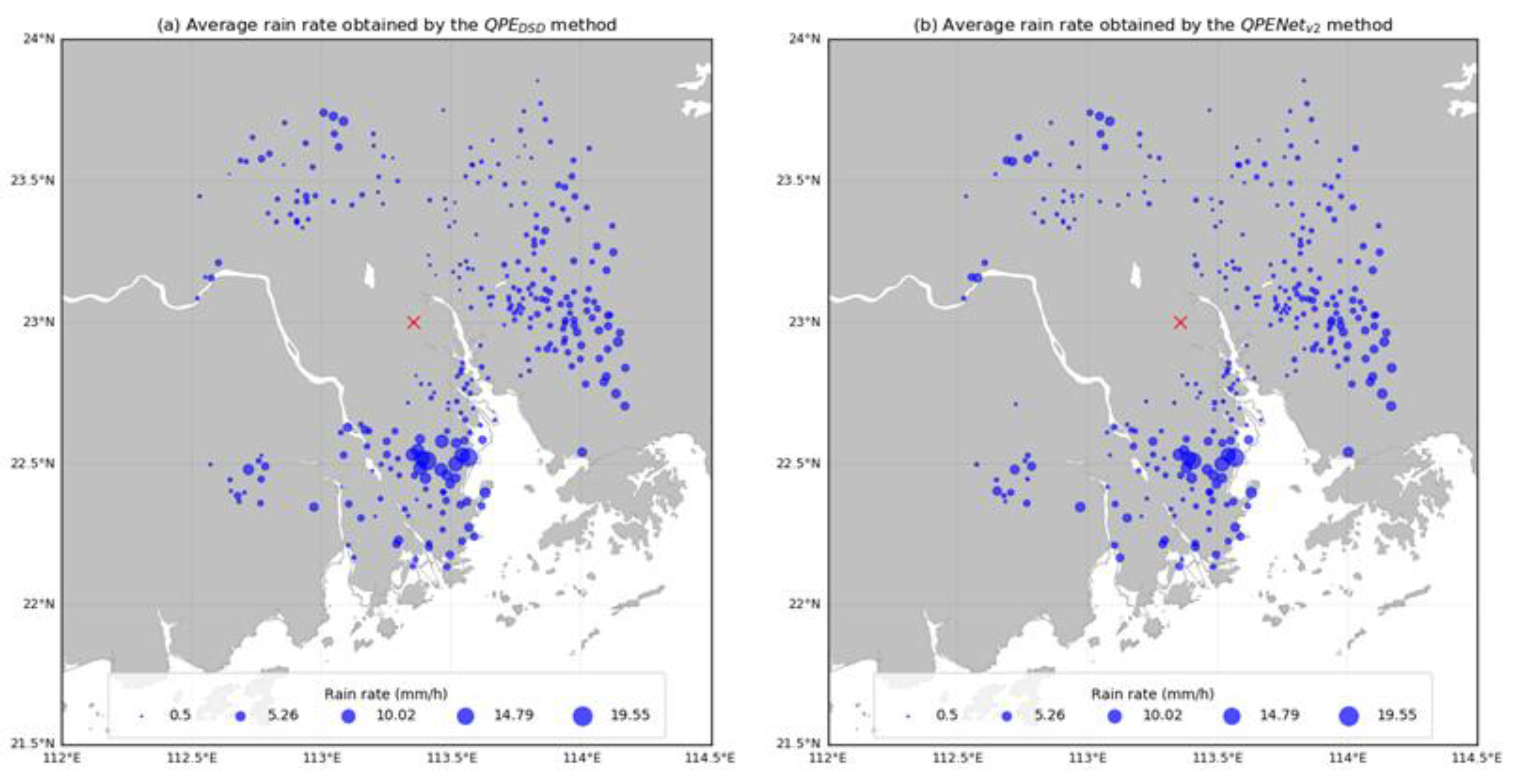
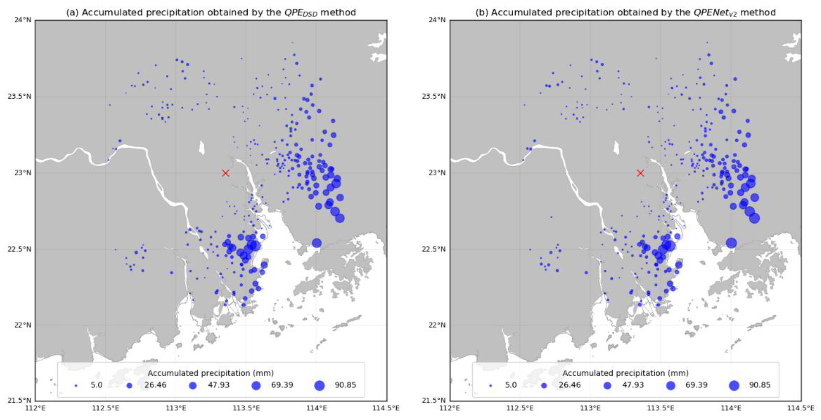
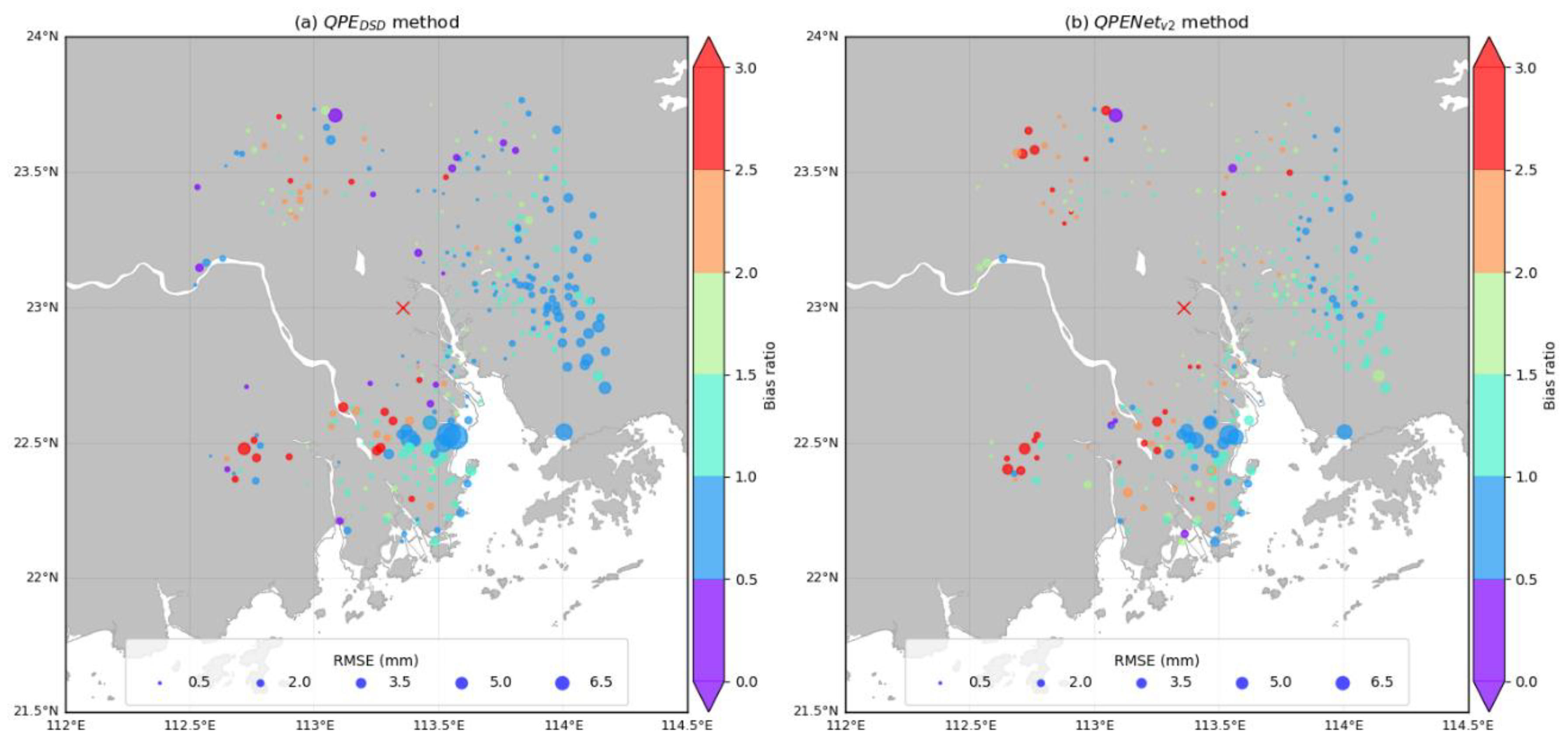
5.3. Spatial Distribution of the Errors Associated with QPEDSD and QPENetV2

The performance of QPEDSD and QPENetV2 was further analyzed in terms of the spatial distribution of the bias ratio and RMSE of the estimated precipitation (Figure 11). As can be seen, the large bias ratios were mainly distributed around 22.4°N 112.75°E, which is due to the partial beam blockage of the Guangzhou radar (i.e., the beam in this area is blocked by an iron tower). The large RMSE areas were mainly distributed in two areas near 22.5°N 113.5°E and 23.1°N 114°E, where the intense rainfall was located (see Figure 6). Overall, the bias ratios and RMSEs of the QPENetV2 algorithm were smaller than those of QPEDSD. Especially around 22.6°N 113.25°E, the bias ratio of QPENetV2 was much smaller. In addition, the RMSE of QPENetV2 was much smaller around 23.1°N 114°E, further demonstrating that the QPENetV2 algorithm had better performance.

6. Concluding Remarks

For this study, we designed a deep neural network algorithm termed QPENet for polarimetric radar QPE. To train this deep-learning model, three versions of the “DPO—SR” dataset were constructed using observations from the radar and AWS during eleven typhoon events in South China. Through evaluation and comparison with the traditional QPEDSD method using the test event, the performance and applicability of QPENet were investigated. In order to quantify the influence of the radar observation range on QPE, three datasets of “DPO—SR” were constructed based on the radar observational areas aloft. In particular, 13 × 13, 25 × 25, and 41 × 41 radar range bins centered by the range bin right on top of the AWS were used to match the AWS measurements in constructing the three datasets. Accordingly, three versions of the QPENet model were then trained. The primary findings are summarized as follows.
(1) Based on the evaluation results for all the rainfall intensities during typhoon Merbok, the new QPENet method has better performance than QPEDSD. The overall CC, RMSE, NB, NE, and bias ratio improved by 0.2%, 39%, 73%, 17%, and 73%, respectively, demonstrating the promising performance of the proposed algorithm.
(2) The evaluation results for different (hourly) rainfall intensities during typhoon Merbok also show that QPENet is superior to QPEDSD for most rain intensities. When 5 mm·h−1R < 30 mm·h−1, the CC, RMSE, NB, NE, and bias ratio improved by –1%, 32%, 96%, 31%, and 96%, respectively. When R ≥ 30 mm·h−1, the CC, RMSE, NB, NE, and bias ratio improved by 4%, 47%, 34%, 34%, and 34%, respectively. Only when R < 5 mm·h−1, the QPEDSD algorithm performed similarly to QPENet, which was likely due to the large measurement uncertainty of ZDR and KDP in weak precipitation.
(3) Among the three versions of QPENet, QPENetV2 has the best overall performance, suggesting that the areal radar observations within ~3 km from the AWS location can represent the pointwise surface precipitation the best. Although more experiments are required to further demonstrate this, we can interpret such results from two aspects: on the one hand, during the precipitation particle falling processes, the particle location drift from the radar range gate aloft to the surface can be as large as several kilometers, especially when the wind is strong. Using a 3 km area could resolve the drift fairly well (better than a 1.5 km area); on the other hand, we should not use an area that is too large to capture the fine structure of precipitation. Based on the results in this study, we conclude that 5 km may be too large to represent high-intensity precipitation gradients, resulting in reduced performance in rainfall-mapping heavy-rain regions. However, when R < 5 mm·h−1, the QPENetV3 algorithm performed the best because light rain falls to the surface in a wider area due to the wind effect. In this case, surface precipitation is more correlated with areal radar observations within ~5 km from the AWS.
(4) The performance of the QPEDSD and QPENetV2 algorithms was analyzed by using the bias ratio and RMSE on different segments of ZH, ZDR, and KDP. Overall, in most cases, both Figure 9 and Figure 10 show that the bias ratios of QPENetV2 were smaller than those of QPEDSD. Only when ZH was large and ZDR or KDP was small, the bias ratios of QPEDSD were slightly smaller than those of QPENetV2. Figure 9 and Figure 10 show that the RMSEs of QPENetV2 were smaller than those of QPEDSD in both Figure 9 and Figure 10; only when ZH, ZDR, and KDP were large, the RMSEs of the two algorithms were both large, indicating that there is room for improvement in the stability of the two algorithms. In general, the QPENetV2 algorithm is better than QPEDSD.
(5) The performance of the QPEDSD and QPENetV2 algorithms was further investigated by using the spatial distribution of the bias ratios and RMSEs. In the area around 22.4°N 112.75°E in Figure 11, the bias ratios of the two methods were both large, which may have been caused by the partial beam blockage of the radar. Near 22.5°N 113.5°E and 23.1°N 114°E, the RMSE was larger, which was caused by the larger hourly rainfall intensity (Figure 6). In general, the bias ratio and RMSE of the QPENetV2 algorithm were both smaller and its performance was better than those of QPEDSD.
In summary, the QPENet algorithm has a better performance to estimate surface rainfall intensity from polarimetric radar observations. When precipitation intensity is greater than or equal to 30 mm/h, the advantage of the QPENet algorithm is especially obvious. Nevertheless, the current QPENet algorithm is greatly affected by the quality of radar data. For example, when the rain intensity is less than 5 mm·h−1, the observational error of ZDR and KDP may be large, resulting in a large bias ratio of the QPENet algorithm. In addition, the limited amount of training and test data could have a negative impact on the performance of the QPENet algorithm. To address this, we need to extend the application to cover a variety of severe precipitation events for both training and testing.

Author Contributions

Conceptualization, L.L., S.B. and Y.Z. (Yonghua Zhang); methodology, L.L., Y.Z. (Yonghua Zhang) and H.C.; formal analysis, Y.Z. (Yonghua Zhang), P.S. and Y.Z. (Yang Zhang); resources, Y.Z. (Yi Zhang); data curation, F.Y.; writing—original draft preparation, Y.Z. (Yonghua Zhang), H.C. and P.S.; writing—review and editing, H.C., S.B. and S.Y.; project administration, Y.W.; visualization, Y.Z. (Yonghua Zhang); validation, Y.Z. (Yang Zhang), funding acquisition, Y.Z. (Yi Zhang). All authors have read and agreed to the published version of the manuscript.

Funding

This research was jointly funded by the Key-Area Research and Development Program of Guangdong Province (grant No. 2020B0101130021), the National Key R&D Program of China (grant Nos. 2018YFC1507401 and 2019YFC1510203), and the National Natural Science Foundation of China (grant No. 41971340). The work of H.C. and S.Y. was supported by Colorado State University.

Institutional Review Board Statement

Not applicable.

Informed Consent Statement

Not applicable.

Data Availability Statement

Not applicable.

Acknowledgments

We would like to thank Guangdong Meteorological Service for collecting and archiving the dual-polarization radar and automatic weather station data used in this study.

Conflicts of Interest

The authors declare no conflict of interest.

References

  1. Yin, J.; Yin, Z.; Xu, S. Composite risk assessment of typhoon-induced disaster for China’s coastal area. Nat. Hazards 2013, 69, 1423–1434. [Google Scholar] [CrossRef]
  2. Bringi, V.N.; Chandrasekar, V. Polarimetric Doppler Weather Radar: Principles and Applications; Cambridge University Press: Cambridge, UK, 2001; pp. 635–636. [Google Scholar]
  3. Chen, H.; Chandrasekar, V.; Tan, H.; Cifelli, R. Rainfall Estimation From Ground Radar and TRMM Precipitation Radar Using Hybrid Deep Neural Networks. Geophys. Res. Lett. 2019, 46, 10669–10678. [Google Scholar] [CrossRef]
  4. Cifelli, R.; Chandrasekar, V.; Chen, H.; Johnson, L.E. High Resolution Radar Quantitative Precipitation Estimation in the San Francisco Bay Area: Rainfall Monitoring for the Urban Environment. J. Meteorol. Soc. Jpn. 2018, 96, 141–155. [Google Scholar] [CrossRef] [Green Version]
  5. Gou, Y.; Ma, Y.; Chen, H.; Wen, Y. Radar-derived quantitative precipitation estimation in complex terrain over the eastern Tibetan Plateau. Atmos. Res. 2018, 203, 286–297. [Google Scholar] [CrossRef]
  6. Xia, Q.; Zhang, W.; Chen, H.; Lee, W.-C.; Han, L.; Ma, Y.; Liu, X. Quantification of Precipitation Using Polarimetric Radar Measurements during Several Typhoon Events in Southern China. Remote Sens. 2020, 12, 2058. [Google Scholar] [CrossRef]
  7. Ryzhkov, A.V.; Schuur, T.J.; Burgess, D.W.; Heinselman, P.L.; Giangrande, S.E.; Zrnic, D.S. The joint polarization experiment: Polarimetric rainfall measurements and hydrometeor classification. Bull. Am. Meteorol. Soc. 2005, 86, 809–824. [Google Scholar] [CrossRef] [Green Version]
  8. Xiao, R.; Chandrasekar, V. Development of neural network based algorithm for rainfall estimation based on radar measurements. IEEE Trans. Geosci. Remote Sens. 1997, 35, 160–171. [Google Scholar] [CrossRef] [Green Version]
  9. Chen, H.; Chandrasekar, V.; Cifelli, R. A Deep Learning Approach to Dual-Polarization Radar Rainfall Estimation. In Proceedings of the 2019 URSI Asia-Pacific Radio Science Conference (AP-RASC), New Delhi, India, 9–15 March 2019; pp. 1–2. [Google Scholar] [CrossRef]
  10. Xu, G.; Chandrasekar, V. Operational Feasibility of Neural-Network-Based Radar Rainfall Estimation. IEEE Geosci. Remote Sens. Lett. 2005, 2, 13–17. [Google Scholar] [CrossRef]
  11. Vulpiani, G.; Giangrande, S.; Marzano, F.S. Rainfall estimation from polarimetric S-band radar measurements: Validation of a neutral netwrok approach. J. Appl. Meteorol. Climatol. 2009, 48, 2022–2036. [Google Scholar] [CrossRef]
  12. Dolan, B.; Fuchs, B.; Rutledge, S.A.; Barnes, E.; Thompson, E.J. Primary Modes of Global Drop Size Distributions. J. Atmos. Sci. 2018, 75, 1453–1476. [Google Scholar] [CrossRef]
  13. Wen, G.; Chen, H.; Zhang, G.; Sun, J. An Inverse Model for Raindrop Size Distribution Retrieval with Polarimetric Variables. Remote Sens. 2018, 10, 1179. [Google Scholar] [CrossRef] [Green Version]
  14. Kitchen, M.; Brown, R.; Davies, A.G. Real-time correction of weather radar data for the effects of bright band, range and orographic growth in widespread precipitation. Q. J. R. Meteorol. Soc. 1994, 120, 1231–1254. [Google Scholar] [CrossRef]
  15. Steiner, M.; Smith, J.A. Reflectivity, Rain Rate, and Kinetic Energy Flux Relationships Based on Raindrop Spectra. J. Appl. Meteorol. 2000, 39, 1923–1940. [Google Scholar] [CrossRef]
  16. Kirstetter, P.-E.; Gourley, J.J.; Hong, Y.; Zhang, J.; Moazamigoodarzi, S.; Langston, C.; Arthur, A. Probabilistic precipitation rate estimates with ground-based radar networks. Water Resour. Res. 2015, 51, 1422–1442. [Google Scholar] [CrossRef]
  17. Chen, H.; Chandrasekar, V.; Bechini, R. An Improved Dual-Polarization Radar Rainfall Algorithm (DROPS2.0): Application in NASA IFloodS Field Campaign. J. Hydrometeorol. 2017, 18, 917–937. [Google Scholar] [CrossRef]
  18. Hinton, G.E.; Salakhutdinov, R.R. Reducing the Dimensionality of Data with Neural Networks. Science 2006, 313, 504–507. [Google Scholar] [CrossRef] [PubMed] [Green Version]
  19. LeCun, Y.; Bengio, Y.; Hinton, G. Deep learning. Nature 2015, 521, 436–444. [Google Scholar] [CrossRef] [PubMed]
  20. Han, L.; Zhao, Y.; Chen, H.; Chandrasekar, V. Advancing Radar Nowcasting Through Deep Transfer Learning. IEEE Trans. Geosci. Remote Sens. 2021, in press. [Google Scholar] [CrossRef]
  21. Chen, H.; Chandrasekar, V.; Cifelli, R.; Xie, P. A Machine Learning System for Precipitation Estimation Using Satellite and Ground Radar Network Observations. IEEE Trans. Geosci. Remote Sens. 2019, 58, 982–994. [Google Scholar] [CrossRef]
  22. Tan, H.; Chandra, C.V.; Chen, H. A Deep Neural Network Model for Rainfall Estimation Using Polarimetric WSR-88DP Radar Observations. American Geophysical Union, Fall Meeting, 2016, abstract #IN11B-1622. Available online: https://agu.confex.com/agu/fm16/meetingapp.cgi/Paper/196830 (accessed on 1 June 2021).
  23. Tan, H.; Chandrasekar, V.; Chen, H. A Machine Learning Model for Radar Rainfall Estimation Based on Gauge Observations. In Proceedings of the 2017 United States National Committee of URSI National Radio Science Meeting (USNC-URSI NRSM), Montreal, QC, Canada, 19–26 August 2017; pp. 1–2. [Google Scholar] [CrossRef]
  24. Chen, H.; Chandrasekar, V.; Cifelli, R.; Xie, P.; Tan, H. A data fusion system for accurate precipitation estimation using satellite and ground radar observations: Urban scale application in Dallas-Fort Worth Metroplex. In Proceedings of the 2017 XXXIInd General Assembly and Scientific Symposium of the International Union of Radio Science (URSI GASS), Montreal, QC, Canada, 19–26 August 2017; pp. 1–2. [Google Scholar] [CrossRef]
  25. Chandrasekar, V.; Tan, H.; Chen, H. A machine learning system for rainfall estimation from spaceborne and ground radars. In Proceedings of the 2017 XXXIInd General Assembly and Scientific Symposium of the International Union of Radio Science (URSI GASS), Montreal, QC, Canada, 19–26 August 2017; pp. 1–2. [Google Scholar] [CrossRef]
  26. Moraux, A.; Dewitte, S.; Cornelis, B.; Munteanu, A. Deep Learning for Precipitation Estimation from Satellite and Rain Gauges Measurements. Remote Sens. 2019, 11, 2463. [Google Scholar] [CrossRef] [Green Version]
  27. Wu, C.; Liu, L.; Wei, M.; Xi, B.; Yu, M. Statistics-based optimization of the polarimetric radar hydrometeor classification algorithm and its application for a squall line in South China. Adv. Atmos. Sci. 2018, 35, 296–316. [Google Scholar] [CrossRef]
  28. Wang, Y.; Chandrasekar, V. Algorithm for Estimation of the Specific Differential Phase. J. Atmos. Ocean. Technol. 2009, 26, 2565–2578. [Google Scholar] [CrossRef]
  29. Gou, Y.; Liu, L.; Yang, J.; Wu, C. Operational application and evaluation of the quantitative precipitation estimates algorithm based on the multi–radar mosaic. Acta Meteorol. Sin. 2014, 72, 731–748. (In Chinese) [Google Scholar]
  30. Krizhevsky, A.; Sutskever, I.; Hinton, G.E. Imagenet classification with deep convolutional neural networks. Adv. Neural Inf. Process. Syst. 2012, 25, 1097–1105. [Google Scholar] [CrossRef]
  31. Szegedy, C.; Liu, W.; Jia, Y.; Sermanet, P.; Reed, S.; Anguelov, D.; Erhan, D.; Vanhoucke, V.; Rabinovich, A. Going deep-er with convolutions. In Proceedings of the IEEE Conference on Computer Vision and Pattern Recognition, Boston, MA, USA, 7–12 June 2015; pp. 1–9. [Google Scholar] [CrossRef] [Green Version]
  32. He, K.; Zhang, X.; Ren, S.; Sun, J. Deep Residual Learning for Image Recognition. In Proceedings of the IEEE Conference on Computer Vision and Pattern Recognition (CVPR), Las Vegas, NV, USA, 27–30 June 2016; pp. 770–778. [Google Scholar] [CrossRef] [Green Version]
  33. Liu, Y.; Minh Nguyen, D.; Deligiannis, N.; Ding, W.; Munteanu, A. Hourglass-shapenetwork based semantic segmentation for high resolution aerial imagery. Remote Sens. 2017, 9, 522. [Google Scholar] [CrossRef] [Green Version]
  34. Glorot, X.; Bengio, Y. Understanding the difficulty of training deep feedforward neural networks. In Proceedings of the Thirteenth International Conference on Artificial Intelligence and Statistics Intelligence and Statistics, Sardinia, Italy, 13–15 May 2010; pp. 249–256. [Google Scholar]
  35. Zhang, Y.; Liu, L.; Bi, S.; Wu, Z.; Shen, P.; Ao, Z.; Chen, C.; Zhang, Y. Analysis of Dual-Polarimetric Radar Variables and Quantitative Precipitation Estimators for Landfall Typhoons and Squall Lines Based on Disdrometer Data in Southern China. Atmosphere 2019, 10, 30. [Google Scholar] [CrossRef] [Green Version]
  36. Zhang, Y.; Liu, L.; Wen, H.; Wu, C.; Zhang, Y. Evaluation of the Polarimetric-Radar Quantitative Precipitation Estimates of an Extremely Heavy Rainfall Event and Nine Common Rainfall Events in Guangzhou. Atmosphere 2018, 9, 330. [Google Scholar] [CrossRef] [Green Version]
Figure 1. Tracks of the eleven landfalling typhoons and the locations of the Guangzhou radar (red cross) and automatic weather stations. The blue triangles and black dots denote the national automatic weather stations and regional automatic weather stations between the 15 km and 100 km coverage ranges (two black circles) of the Guangzhou radar.
Remotesensing 13 03157 g001
Figure 2. Construction of data samples for machine learning. D is the distance from the automatic weather stations to the radar; (4), (3), (2), and (1) represent the fourth, third, second, and first scan elevation angles of the radar, respectively.
Remotesensing 13 03157 g002
Figure 3. Simplified flowchart of the QPENet model structure and its application for polarimetric radar quantitative precipitation estimation.
Remotesensing 13 03157 g003
Figure 4. Detailed architecture of the proposed model. Each convolutional layer is followed by a batch normalization layer, and the ReLU is used as the activation function.
Remotesensing 13 03157 g004
Figure 5. Diagram of the Inception module. The filter numbers used for each layer are given in Table 3.
Remotesensing 13 03157 g005
Figure 6. Hourly rainfall estimates using (a) QPEDSD and (b) QPENetv2 during typhoon Merbok. The red cross represents the location of the Guangzhou radar.
Remotesensing 13 03157 g006
Figure 7. The same as Figure 6, but for the accumulated rainfall during the whole event.
Remotesensing 13 03157 g007
Figure 8. Scatterplots of rainfall estimates from the automatic weather stations versus radar during typhoon Merbok. (ad) QPEDSD. (eh) QPENetV2. (a,e), (b,f), (c,g), and (d,h) correspond to all rainfall intensities, R < 5 mm·h−1, 5 ≤ R < 30 mm·h−1, and 30 mm·h−1R, respectively.
Remotesensing 13 03157 g008
Figure 9. Bubble charts of the bias ratios and RMSEs of the radar-derived hourly rainfall estimates during typhoon Merbok: (a) QPEDSD; (b) QPENetV2. The bias ratios and RMSEs were calculated for different ZH and ZDR ranges using observations from the automatic weather stations as references. ZH is divided into “<20 dBZ”, “20–30 dBZ”, and “≥30 dBZ”. ZDR is divided into “<0.2 dB”, “0.2–0.4 dB”, and “≥0.4 dB”. The size of the dots represents the RMSE, the color of the dots indicates the bias ratio.
Remotesensing 13 03157 g009
Figure 10. Bubble charts of the bias ratios and RMSEs of the radar-derived hourly rainfall estimates during typhoon Merbok: (a) QPEDSD; (b) QPENetV2. The bias ratios and RMSEs were calculated for different ZH and KDP ranges using observations from the automatic weather stations as references. ZH is divided into “<20 dBZ”, “20–30 dBZ”, and “≥30 dBZ”. KDP is divided into “<0.1°·km−1”, “0.1−0.25°·km−1”, and “≥0.25°·km−1”. The size of the dots represents the RMSE, the color of the dots indicates the bias ratio.
Remotesensing 13 03157 g010
Figure 11. The spatial distributions of the bias ratios and RMSEs of hourly rainfall estimates from (a) QPEDSD and (b) QPENetV2 during typhoon Merbok. The bias ratios and RMSEs were calculated based on the automatic weather station observations. The red cross represents the location of the Guangzhou radar. The size of the dots represents the RMSE, the color of the dots indicates the bias ratio.
Remotesensing 13 03157 g011
Table 1. Detailed information on the eleven typhoon precipitation events.
#Name
(No.)
Date (UTC)Total
Time
(h)
No. of
Valued
gauges
No. of
Radar Volumes
Mean Gauge
Accumulation
(mm)
Maximum Gauge
Accumulation
(mm)
1Merbok
(1702)
June 12–13, 20171954419018.32144.4
2Hato
(1713)
August 23, 20171277512025.2254
3Pakhar
(1714)
August 26–27, 201797639044.5471
4Mawar
(1716)
September 02–04, 20172872028031.67211.3
5Khanun
(1720)
October 15–16, 20171876518027.3385.2
6Ewiniar
(1804)
June 07–08, 201837793370212.46311.2
7Bebinca
(1816)
August 10–15, 20181198041190100.48255.6
8Mangkhut
(1822)
September 16, 201897979077.44148.4
9Barijat
(1823)
September 12–13, 2018216132102.9814
10Wipha
(1907)
August 01–02, 20192080620044.62170.4
11Bailu
(1911)
August 24–25, 20192379823045.4999.1
Table 2. Sample information of the “DPO—SR” dataset.
#Name
(No.)
No. of Samples
in Dataset V1
No. of Samples
in Dataset V2
No. of Samples
in Dataset V3
1Merbok (1702)450045024510
2Hato (1713)19,19619,18819,198
3Pakhar (1714)30,39830,40130,405
4Mawar (1716)899589928993
5Khanun (1720)11,89211,88011,884
6Ewiniar (1804)115,703115,737115,726
7Bebinca (1816)63,81863,87463,877
8Mangkhut (1822)47,23047,22047,229
9Barijat (1823)141214121414
10Wipha (1907)32,09732,09932,089
11Bailu (1911)39,93239,93539,942
Total375,173375,240375,267
Table 3. Filter numbers for each convolution type in the Inception module. Note: “n × n Reduce” stands for the 1 × 1 convolutions preceding the corresponding n × n convolutions.
Total # (Filter Output)# 1 × 1# 3 × 3 Reduce# 3 × 3# 5 × 5 Reduce# 5 × 5# 1 × 1
25664128128643232
51265256384643232
Table 4. The hyperparameters of the QPENet model.
Dataset VersionBatch SizeConvergence EpochsLearning RateTime per Epoch (s)Weight Decay
V151220.001114.50.0001
V2512120.001231.20.0001
V3256260.001615.40.0001
Table 5. Evaluated scores for four kinds of QPE algorithms for the Merbok event for all rainfall intensities.
QPE AlgorithmCCRMSENB (%)NE (%)Bias Ratio
QPENetV10.932.154.1438.051.04
QPENeV20.951.757.3233.921.07
QPENetV30.961.97−19.4236.720.81
QPEDSD0.942.87−15.2741.110.85
Table 6. The same as Table 5 except that the rainfall intensity is less than 5 mm·h−1 (R < 5 mm·h−1).
QPE AlgorithmCCRMSENB (%)NE (%)Bias Ratio
QPENetV10.780.9622.2545.101.22
QPENetV20.810.8722.5442.351.23
QPENetV30.740.84−14.1441.580.86
QPEDSD0.681.17−2.8344.420.97
Table 7. The same as Table 5 except that the rainfall intensity is greater than or equal to 5 mm and less than 30 mm (5 ≤ R < 30 mm·h−1).
QPE AlgorithmCCRMSENB (%)NE (%)Bias Ratio
QPENetV10.703.92−5.2229.050.95
QPENeV20.743.67−1.1725.590.99
QPENetV30.764.10−22.7432.700.77
QPEDSD0.775.37−26.9436.970.73
Table 8. The same as Table 5 except that the rainfall intensity is greater than or equal to 30 mm (R ≥ 30 mm·h−1).
QPE AlgorithmCCRMSENB (%)NE (%)Bias Ratio
QPENetV11.0022.03−35.8835.880.64
QPENeV20.9816.01−24.8924.890.75
QPENetV30.9819.24−29.6329.630.70
QPEDSD0.9630.02−37.6737.670.62
Publisher’s Note: MDPI stays neutral with regard to jurisdictional claims in published maps and institutional affiliations.

