Article

Joint Retrieval of Winter Wheat Leaf Area Index and Canopy Chlorophyll Density Using Hyperspectral Vegetation Indices

1
China Aero Geophysical Survey and Remote Sensing Center for Natural Resources, Beijing 100083, China
2
Key Laboratory of Digital Earth Science, Aerospace Information Research Institute, Chinese Academy of Sciences, Beijing 100094, China
3
College of Resources and Environment, University of Chinese Academy of Sciences, Beijing 100190, China
4
State Key Laboratory of Remote Sensing Science, Aerospace Information Research Institute, Chinese Academy of Sciences, Beijing 100094, China
5
Faculty of Science, University of Technology Sydney, Sydney, NSW 2007, Australia
*
Author to whom correspondence should be addressed.
Remote Sens. 2021, 13(16), 3175; https://0-doi-org.brum.beds.ac.uk/10.3390/rs13163175
Submission received: 14 June 2021 / Revised: 4 August 2021 / Accepted: 6 August 2021 / Published: 11 August 2021
(This article belongs to the Special Issue Remote Sensing for Precision Agriculture)

Abstract

:
Leaf area index (LAI) and canopy chlorophyll density (CCD) are key biophysical and biochemical parameters utilized in winter wheat growth monitoring. In this study, we would like to exploit the advantages of three canonical types of spectral vegetation indices: indices sensitive to LAI, indices sensitive to chlorophyll content, and indices suitable for both parameters. In addition, two methods for joint retrieval were proposed. The first method is to develop integration-based indices incorporating LAI-sensitive and CCD-sensitive indices. The second method is to create a transformed triangular vegetation index (TTVI2) based on the spectral and physiological characteristics of the parameters. PROSAIL, as a typical radiative transfer model embedded with physical laws, was used to build estimation models between the indices and the relevant parameters. Validation was conducted against a field-measured hyperspectral dataset for four distinct growth stages and pooled data. The results indicate that: (1) the performance of the integrated indices from the first method are various because of the component indices; (2) TTVI2 is an excellent predictor for joint retrieval, with the highest R2 values of 0.76 and 0.59, the RMSE of 0.93 m2/m2 and 104.66 μg/cm2, and the RRMSE (Relative RMSE) of 12.76% and 16.96% for LAI and CCD, respectively.

Graphical Abstract

1. Introduction

Vegetation-based remote sensing approaches utilizing the leaf area index (LAI) and canopy chlorophyll density (CCD) have provided valuable insights into the spatiotemporal variability of the biophysical and biochemical parameters or traits of plants [1,2]. LAI is calculated as the one-sided leaf area above per unit of the ground area [3]. It is the key biophysical parameter when evaluating agroecosystems. The chlorophyll content is of great importance in the biosphere as a photosynthetic pigment and is used as an intermediate indicator of leaf nitrogen contents, due to their linear correlation [4,5]. CCD represents the multiplication of LAI and leaf chlorophyll density (LCD). Thus, it represents the chlorophyll content at the canopy scale [6]. These values have been used as indicators to evaluate the structural and nutritional conditions of an area to further predict crop yield [7].
Remote sensing technology has become an efficient and useful method for vegetation parameter estimation. There is currently a discussion on the appropriate selection between hyperspectral data and multispectral data. Hyperspectral vegetation indices and their relationships with agricultural crop characteristics, including LAI, leaf chlorophyll content, biomass, and plant height, have been studied thoroughly [8]. Compared with broadband indices, narrowband indices perform better under certain circumstances [9]. The superiority of narrowband index parameter estimation can contribute to its fine resolution. With the growing public attention and demands in precision agriculture, it is vital to acquire accurate crop growth conditions over time. Researchers have performed much work on quantitatively estimating vegetation parameters [10,11,12,13,14,15]. Among the available estimation methods, establishing empirical models between vegetation indices and parameters with statistical relationships is a widely accepted parameter retrieval technique [16,17]. Over the past few decades, various spectral vegetation indices utilizing the spectral response to parameter characteristics have been proposed. Researchers have conducted retrieval methods for various vegetation types and crop types and for multiple remote sensing sensors, and they have also developed methods focused on eliminating interfering factors such as soil background, atmospheric conditions, and canopy structure effects [18,19,20,21,22]. For example, the normalized difference vegetation index (NDVI) is the cornerstone of the vegetation indices used to estimate LAI variations, with the normalized difference between the red and near-infrared reflectance bands [23]. Considering that they become saturated under a high foliage cover, the transformed triangular vegetation index (TTVI) was proposed to reduce the saturation effect for LAI retrieval by utilizing the triangular area embraced by LAI-sensitive bands [24]; in addition, the modified soil-adjusted vegetation index (MSAVI) eliminated the effects of chlorophyll on the LAI by adding a self-adjusted factor [25]. The optimized soil-adjusted vegetation index (OSAVI) minimized the impact of soil by adding an adjusting factor [26]; the modified triangular vegetation index (MTVI2) was found to be sensitive to LAI variations but resistant to leaf chlorophyll contents [17]. The chlorophyll index (CI) and MERIS terrestrial chlorophyll index (MTCI) were shown to be good chlorophyll indicators using chlorophyll-sensitive wavelengths before 600 nm [27], and the integrated vegetation index RECAI/TVI, which combines the red-edge chlorophyll absorption index and the modified triangular vegetation index, was proposed to estimate leaf chlorophyll contents. It is also able to reduce the effect of the LAI [28]. Parts of these indices have also been used for winter wheat parameter retrieval. In summary, the research basis for improving parameter retrieval accuracy is solid and sufficiently supported.
The increasing number of indices enriches the choices available for quantitatively estimating vegetation parameters. However, with the development of a growing demand for accurate and fast quantitative remote sensing techniques, a variety of problems in vegetation retrieval have emerged. For example, the lack of indices for joint retrieval needs to be determined. LAI and CCD together reflect the vegetation density, vitality and photosynthetic potential of an area [29]. Most published estimation models or vegetation indices focus on how to improve retrieval accuracy. However, another key point is that the single retrieval of biophysical or biochemical parameters is unilateral. No single parameter can interpret the condition of crops in all aspects. It would be efficient and comprehensive if there were a method available to capture both biochemical and biophysical information from both sides, based on the variation of winter wheat LAI and CCD at different growth stages. The regularized canopy reflectance model (REGFLEC) has inspired us to explore jointly retrieving parameters [30]. The model utilized automated image-based methodologies and was developed to incorporate space observations to exploit LAI and chlorophyll information that is derived from multiple satellite scenes [30]. It produces both LAI and chlorophyll estimations at the same time. Another group of joint retrieval methods comes from the crop status index (CSI). A minimum dataset was selected from twenty crop abiotic stress indicators and was then scored linearly or nonlinearly to form the index. Actually, the CSI is an integration of indicators and can be used for distinguishing and evaluating the types of composition stress [29]. An index used to estimate both parameters at the same time could also improve retrieval efficiency. Combining the advantages of indices and exploiting them for wider application in remote sensing can be considered a “reuse” of these indices.
One possible method for the joint retrieval of LAI and CCD is to integrate existing vegetation indices that are sensitive to biophysical and biochemical parameters, respectively. The same method has been used for the prediction of crop chlorophyll contents and has made great progress [31]. Theoretically, the multiplication of two kinds of indices could be used to combine information from both sides. However, due to the specific conditions, the sensitive wavelengths and index forms might harm the resulting accuracy. In this case, taking advantage of both sides introduces uncertainty. Notably, CCD is the multiplication of the LAI and the LCD, but LAI-sensitive or LCD-sensitive indices might not be able to show a good correlation with the CCD. There is a possibility that the multiplication of two indices leads to the suppression of one of the evaluated parameters. Another method used for the joint retrieval of LAI and CCD is to propose a new index specialized for joint retrieval. The LAI and CCD both exert influences on vegetation spectral reflectance, but at different spectral regions. Research on the red-edge spectral region indicates that the retrieval accuracy of both LAI and CCD can be improved [32,33]. The red-edge inflection point (REIP) moves toward longer wavelengths under a high vegetation cover or a high chlorophyll content, while moving backward toward shorter wavelengths under a low vegetation cover or when the leaves are withered. This shift of the REIP can be used not only for growth stage monitoring but also for nutritional status, crop biomass, and, furthermore, crop yield determinations [34,35]. Therefore, spectral bands from the red-edge region can be a good option for joint retrieval of winter wheat LAI and CCD.
The simultaneous retrieval of winter wheat LAI and CCD is challenging but promising. The joint retrieval of biophysical and biochemical parameters can be an efficient and cost-effective method to monitor crop growth conditions. Thus, the objectives of this study are: (1) to select optimal indices that are sensitive to LAI or chlorophyll variations for integration-based index development; (2) to propose a new index for joint retrieval based on the response patterns of spectral reflectance to biophysical and biochemical parameters; (3) to validate the proposed joint retrieval methods with field-measured data and to compare the estimation capabilities of new indices against other existing indices at the key growth stages of winter wheat.

2. Materials and Methods
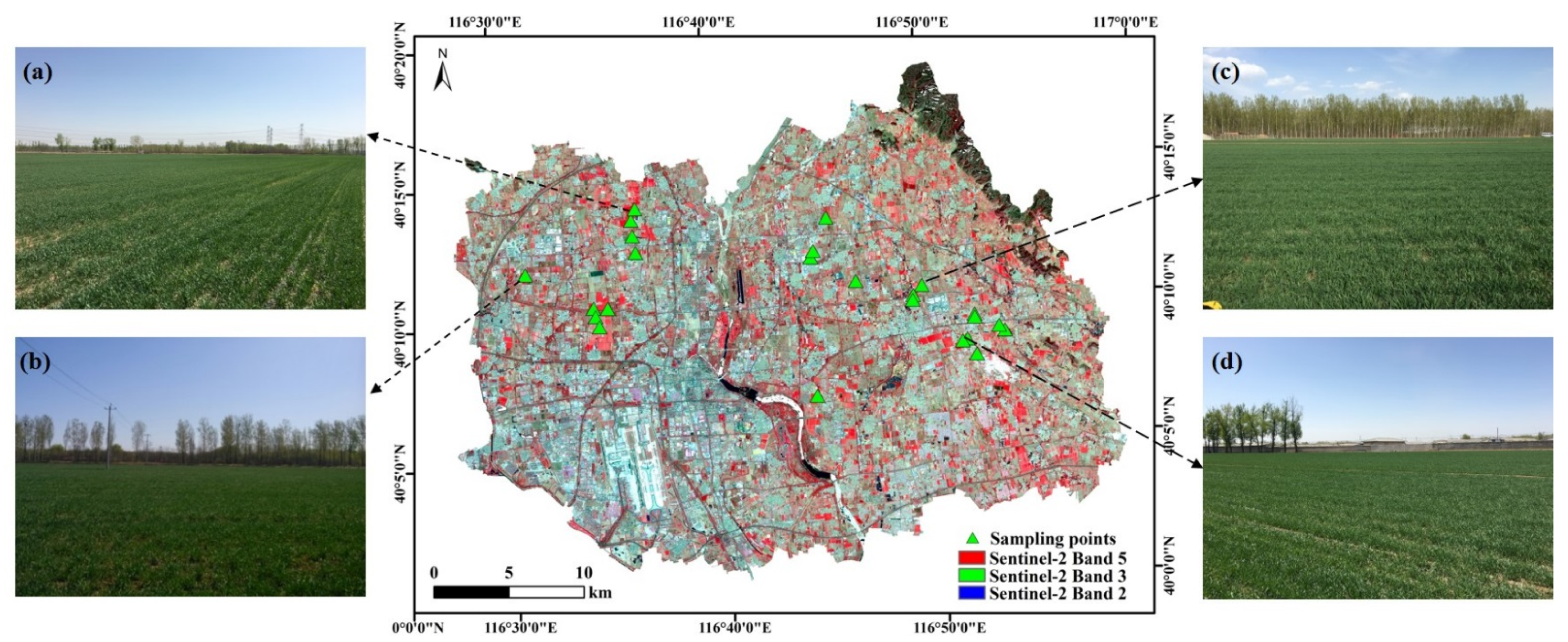
2.1. Study Area

Winter wheat is one of the most essential cereals in the world and is the research object of our study. The study site was located on winter wheat farmland in Shunyi District, Beijing (116°31′10″E to 116°53′26″E, 40°8′2″N to 40°14′0″N) in 2016 during the growing season. The study area is located on the Northern China Plain, with an average annual temperature of 13.8 °C. The field measurements were conducted during four specific growth stages: early jointing stage, late jointing stage, head emergence stage, and filling stage. There were twenty-four sampling units with an average size of more than 3 ha (the distribution of the sampling units is shown in Figure 1). A total of 96 plots were measured, each covering a square plot sized 1 m × 1 m. The sampling site consisted of continuous winter wheat farmland, and the growth conditions varied due to the application of various water- and fertilizer-management strategies. To eliminate the measuring errors of the field-collected data, the sampling plots were divided into four parts: northwest, northeast, southwest and southeast. There were 6 sampling plots in each area. After that, three-quarters of the measurements from each part were chosen randomly via MATLAB. Thus, 18 measurements at each growth stage were selected (the description of sample plots used at each growth stage is listed in Table 1). These data were pooled for validation in Section 3.3.

2.2. Field Measurements

Both biophysical and biochemical parameters, including the LAI and the CCD, were collected during field campaigns. A total of 96 LAI measurements were collected in each sample plot with the Plant Canopy Analyzer instrument LAI-2200c (LI-COR Inc., Lincoln, NE, USA). Fifteen whole winter wheat plants were pulled from the soil at each sampling point and were quickly moved into a cooler box with ice, in case of water loss. After all the samples from 24 points were collected, they were moved to the laboratory for further analyses. The laboratory analyses of the LCC were conducted according to standard processes [16,36,37]. The corresponding weights and area of sampling leaves were then used to transfer the LCC to leaf chlorophyll density (LCD, μg/cm2) [16]. Finally, canopy chlorophyll density (CCD) was calculated by multiplying the LAI and the LCD.
Together with parameter value collection, canopy reflectance collection was carried out using an ASD FieldSpec spectrometer (Analytical Spectral Devices, Inc., Boulder, CO, USA) simultaneously during field measurements. The spectrometer was configured with a spectral range of 350–2500 nm, with a field of view of 25°. Measurements were obtained from a nadir position at approximately 1.3 m above the ground and averaged by 10 repeated scans. For each sampling plot, an approximate area of 1 m2 was collected. The hyperspectral spectrum was calibrated by a 0.4 m × 0.4 m white reference panel, both before and after plant canopy measurements. To minimize the noise from the water and carbon dioxide components of the canopy spectra, only the spectral bands from 400 nm to 2500 nm were used in the research. The spectral resolution was 3 nm for wavelengths ranging from 350 to 1000 nm, and 10 nm for wavelengths from 1000 to 2500 nm.

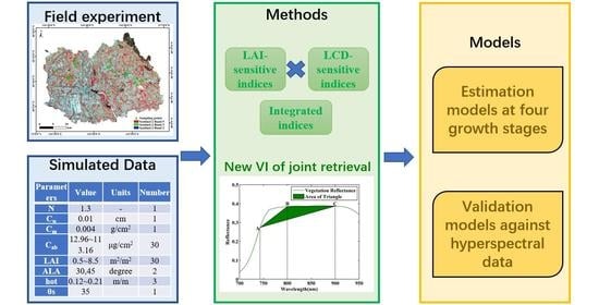
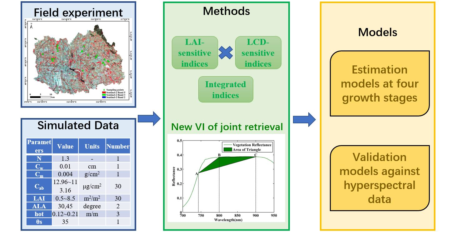
2.3. Simulated Spectral Datasets

To enrich the datasets, the PROSAIL-5 model was used in this study to analyze the sensitivity between spectral reflectance and vegetation parameters. PROSAIL is a typical radiation transfer model (RTM) that is based on physical laws and establishing cause-effect relationships [38]. It is the coupled model of the PROSPECT5B leaf reflectance model and the 4SAIL (scattering by arbitrary inclined leaves) canopy reflectance model, which are able to simulate the vegetation reflectance at the canopy level [39]. PROSPECT simulates reflectance and transmittance at the leaf level. The parameter settings in this research referred to the ranges of the field-measured vegetation parameters of winter wheat in 2016 (shown in Table 2), and relevant studies were also taken into consideration [17,40,41,42]. A total of 5400 sets were generated randomly, based on the parameter settings of the PROSAIL model. The aim of such a database is to test the estimation abilities of the model using a vast number of spectral reflectance that represent possible biochemical and biophysical properties for winter wheat, which is rarely achieved in field experiments.

2.4. Methods for Joint Retrieval

Two methods of joint retrieval are used in the manuscript. The first method is to select existed indices that have been widely utilized for the retrieval of LAI or CCD, and then compare their abilities regarding joint retrieval; the second method aims to create a joint-retrieval-specific index, making use of the above-mentioned indices.

2.4.1. Vegetation Indices Used for Integration-Based Indices

The vegetation indices used in this study can be categorized into three main classes: (1) indices sensitive to LAI; (2) indices sensitive to chlorophyll content; and (3) indices sensitive to both LAI and chlorophyll content. Integration-based indices were further proposed based on these three types of indices. When selecting the indices, three factors are considered: (1) the index has to be sensitive to LAI or CCD, or to both parameters; (2) the index is resistant to at least one interfering factor; (3) the index can be calculated with hyperspectral remote sensing data.
(1) Indices sensitive to LAI
The retrieval of LAI can be affected by atmospheric scattering and absorption effects, saturation effects, temporal effects, and soil background effects [43]. DVI, NDVI, TVI, TTVI, and MSAVI are selected as indices sensitive to LAI. NDVI is a fundamental index used in quantitative vegetation remote sensing. It utilizes the ratio of near-infrared and red bands to monitor the LAI variation but suffers from the saturation effect problem [23]. The retrieval accuracy is hindered by high vegetation cover. The triangular vegetation index (TVI) and its transformed counterparts and TTVI have been suggested as being sensitive to LAI and resistant to CCD for winter wheat [24,25]. The soil-adjusted vegetation index (SAVI) and its family indices, including MSAVI, use interfering factors to eliminate noise from the soil background and improve the LAI retrieval accuracy [26]. MSAVI also exhibited good LAI estimations for winter wheat LAI with ground-measured hyperspectral data [44].
(2) Indices sensitive to chlorophyll content
The first derivative and reciprocal reflectance are useful for chlorophyll retrieval [45]. In this class, PSSRa, CIred-edge, RES, and MCARI were selected. PSSRa indicates the chlorophyll-a concentration in the plant [23]. It presented a significant phenotypic correlation with winter wheat chlorophyll concentration (SPAD unit) at the heading and milk development stages in the previous study [46]. The chlorophyll index (CI) and its revisions, i.e., CIred-edge and CIgreen, take advantage of reciprocal data and show great potential in the remote tracking of the physiological status of crops, including maize and soybean [47,48]. CIred-edge was linearly related to the canopy chlorophyll content with hyperspectral remote sensing data, due to the sensitivity of the red edge to chlorophyll contents [14]. Red edge symmetry (RES) is an easily calculated index and is applicable to hyperspectral data [33]. Its ability to retrieve chlorophyll data meets our research goal in this study. Thus, we decided to use it as a chlorophyll-sensitive index. MCARI was proved to have better linearity with winter wheat and corn chlorophyll content [49].
(3) Indices capable for both parameters
The leaf chlorophyll level can affect LAI retrieval by affecting the canopy’s optical properties [43]. Thus, few indices have been designed to estimate both biophysical and biochemical parameters. The photochemical reflectance index (PRI) was initially proposed for photosynthetic radiation use efficiency [50]. It has also been proved to be sensitive to Cab in soybean and maize at the leaf scale, and sensitive to LAI at the canopy scale [51]. Two wavelengths of PRI 531 nm and 570 nm were utilized, due to their major role in the xanthophyll cycle and the reduction of chloroplast movements.
In this section, the first method of joint retrieval is proposed. It integrates LAI-sensitive indices and chlorophyll-sensitive indices and takes advantage of both sides. Based on the indices selected in Table 3, the integration-based indices in the study are CI-integrated indices, including CIred-edge×NDVI, CIred-edge×TVI, CIred-edge×TTVI, CIred-edge×PSSRa, CIred-edge×MSAVI, CIred-edge×MCARI, CIred-edge×PRI, and RES-integrated indices, including RES×NDVI, RES×TVI, RES×TTVI, RES×PSSRa, RES×MSAVI, RES×MCARI, and RES×PRI.

2.4.2. New Indices for Joint Retrieval

We calculated the Pearson correlation coefficients between the vegetation parameters, including LAI, LCD, and CCD, with PROSAIL simulated spectral reflectance (see Figure 2). As shown in the figure, the sensitive spectral regions are distinct for LAI and LCD. Wavelengths of approximately 640–690 nm are sensitive to LAI variation, and wavelengths near 520–560 nm are better correlated with LCD. However, the multiplication of LCD and LAI, which equals the CCD, takes the mutual advantages of the two parameters and shows a good correlation with two spectral regions before 700 nm. The CCD curve exhibited similar trends with LAI after 700 nm. There was a difference in the correlation between LAI and Cab at approximately 718 nm, which is sensitive to LCD variations but resistant to LAI variations. Wavelengths less than 718 nm are negatively related to Cab. We further discovered the correlation between CCD and the red-edge position in Figure 3. In conclusion, the possible spectral regions for both LAI and CCD are red-edge and NIR regions. The red-edge position is affected by both LAI and chlorophyll concentration [53]. To ensure the sensitivity of CCD to reflectance at approximately 700 nm, we further calculated the correlation of CCD and the red-edge position in Figure 3. The CCD is exponentially related to the red-edge position with an R2 value of 0.758. For now, we were able to count red-edge spectral bands in the new index.
We further tested the sensitivity of wavelength combinations for LAI and CCD with TVI-like indices. The red-edge spectral region ranged from 680 nm to 760 nm, and the two NIR regions were 760 nm to 860 nm and 800 nm to 1000 nm. As shown in Figure 4, the combination of wavelengths for the two parameters is not the same. The selection of the red-edge wavelength is the key point for the index. For the LAI, wavelengths shorter than 740 nm had an r over 0.8, but the situation was the opposite for the CCD. The indices with wavelengths greater than 740 nm exhibited higher correlations. For both parameters, incorporating longer NIR wavelengths is helpful for the index. Spectral band 6 of the Sentinel-2 MSI sensor is located at 743 nm and has been shown to be sensitive to LAI variations using hyperspectral spectra [24]. To establish a new spectral index for winter wheat LAI and CCD estimation, 800 nm was used because it had a relatively high correlation with both parameters (Figure 4). We included this selection of red-edge regions in the new index. The selection of two near-infrared wavelengths referred to the sensitiveness in Figure 4 and previous studies. Most indices use 800 nm to represent NIR information, such as hyperspectral OSAVI [31] and hyperspectral MCARI/OSAVI, and TCARI/OSAVI [14]. To keep the sensitive response to parameters and take advantage of the correlation, we selected 900 nm as another NIR wavelength for the index.
The three wavelengths of the index were determined. We proposed a new index, i.e., the transformed triangular vegetation index 2 (TTVI2), based on the triangular vegetation index. The mathematical mechanism of TTVI2 is the triangular area embraced by the three vertices of the reflectance spectrum, as shown in Figure 5. According to the law of linear algebra [54], the area of the triangle circled by three vertices can be calculated based on the concept of determinants. The Leibniz formula for the determinant of a 2 × 2 matrix is calculated as shown in Equation (1) below.
The area of the parallelogram is the absolute value of the determinant of the matrix formed by the vectors representing the parallelogram’s sides. Thus, the area of the triangle is half that of the parallelogram with the same sides. In this case, the three vertices are located at A (743, R743), B (800, R800), and C (900, R900). The two vectors of AB and AC are 800–743 and R800–R743, and 900–743 and R900–R743, respectively. Thus, the area of the triangle representing the transformed triangular vegetation index 2 (TTVI2) is calculated using Equations (2) and (3):
| a b c d | = ad bc
TTVI = 0.5 × | ( 800 743 ) ( R 800 R 743 ) ( 900 743 ) ( R 900 R 743 ) |
TTVI 2 = 0.5 × [ ( 800 743 ) × ( R 900 R 743 ) ( 900 743 ) × ( R 800 R 743 ) ]

2.5. Vegetation Parameters Estimation and Validation

The indices for joint retrieval were calculated with the PROSAIL simulated datasets. Parameterized expressions, including linear regression, exponential regression, and logarithmic regression, were built between the indices and parameters individually. For each index, the best-fit model is used as the estimation model. The estimation models were subsequently applied for estimating the LAI and CCD with field-measured hyperspectral data at four growth stages. K-fold cross-validation (k = 4) was used to ensure that every measurement was used for analysis. To ensure that the data range covered the condition of winter wheat at various growth stages, 3/4 of the field measurements from each growth stage were selected, as stated in Section 2.1, and used for validation. A total of 72 measurements were used to ensure that the datasets covered specific growth characteristics and avoided errors from field measurements. The results were validated against ground-measured LAI and CCD. The coefficient of determination (R2), root mean square error (RMSE), and relative root mean square error (RRMSE) are common indicators used for evaluating estimation models. The RRMSE is computed as the RMSE, normalized by the measured range of the corresponding parameter [55]. It evaluates the robustness of indices.

3. Results

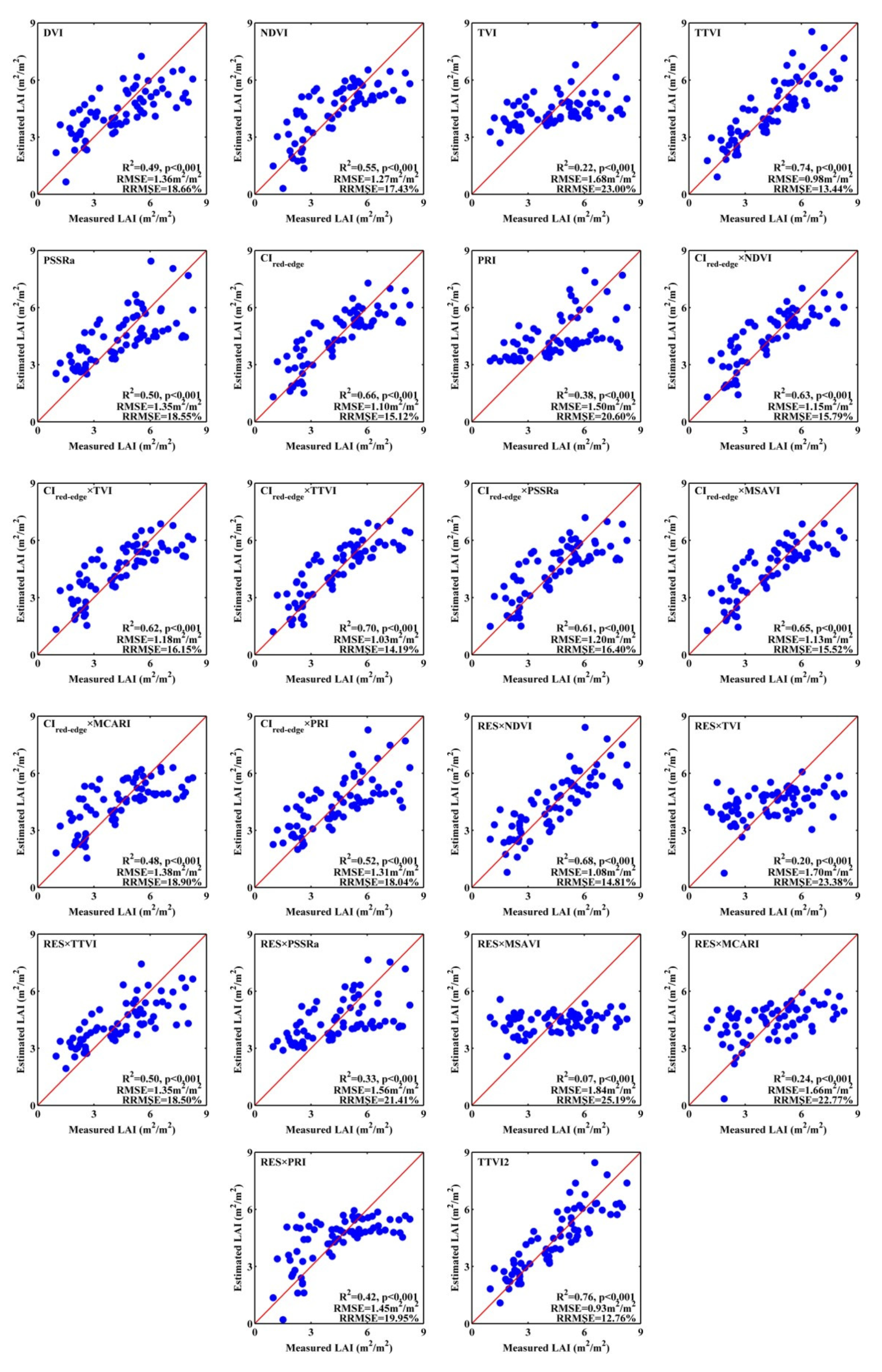
3.1. Estimation Models from PROSAIL Datasets

The estimation models for the PROSAIL-derived indices and parameters are shown in Table 4. It is obvious that the indices from different classes (referred to in Section 2.4.1) performed differently. The three main relationships between indices and parameters are linear, exponential, and logarithmic relationships. It is common for most CIred-edge-integrated indices to be logarithmically related to the LAI and linearly related to the CCD. The classic indices, including DVI, PSSRa, and NDVI, exhibited high correlations with both the LAI and the CCD. TVI is more related to LAI than CCD, and the situation for CIred-edge is the opposite. The situation for integration-based indices can vary. Most integrated indices performed well, with R2 values higher than 0.5, such as PRI, TVI, and the majority of CIred-edge-integrated indices. CIred-edge-integrated indices are also more closely related to the CCD than the LAI. There is no doubt that CIred-edge is a good CCD indicator. However, the RES-integrated indices did not show a satisfactory estimation. Most RES-integrated indices reported R2 values of less than 0.5. The only exception is RES×TTVI, with R2 values of 0.85 and 0.72 for the LAI and CCD, respectively. There was also no obvious commonality between RES-integrated indices. Some of them were more closely related to the CCD, while others were not. The form of the triangular vegetation index plays an influential role in parameter retrieval. TTVI, CIred-edge×TTVI, and RES×TTVI are all good indicators for CCD with relatively high R2. Among them, TTVI2 exhibited the best performance, with the highest R2 value of 0.95. PRI showed good estimation for both LAI and CCD, and it had the highest R2 value with LAI of 0.97 among all the indices.

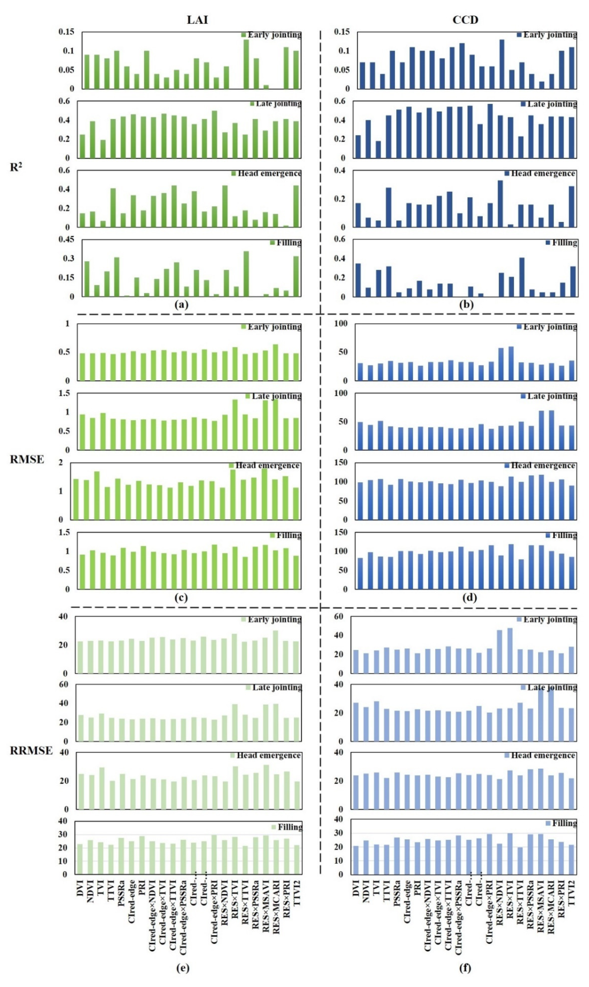
3.2. Estimation Results at Different Growth Stages
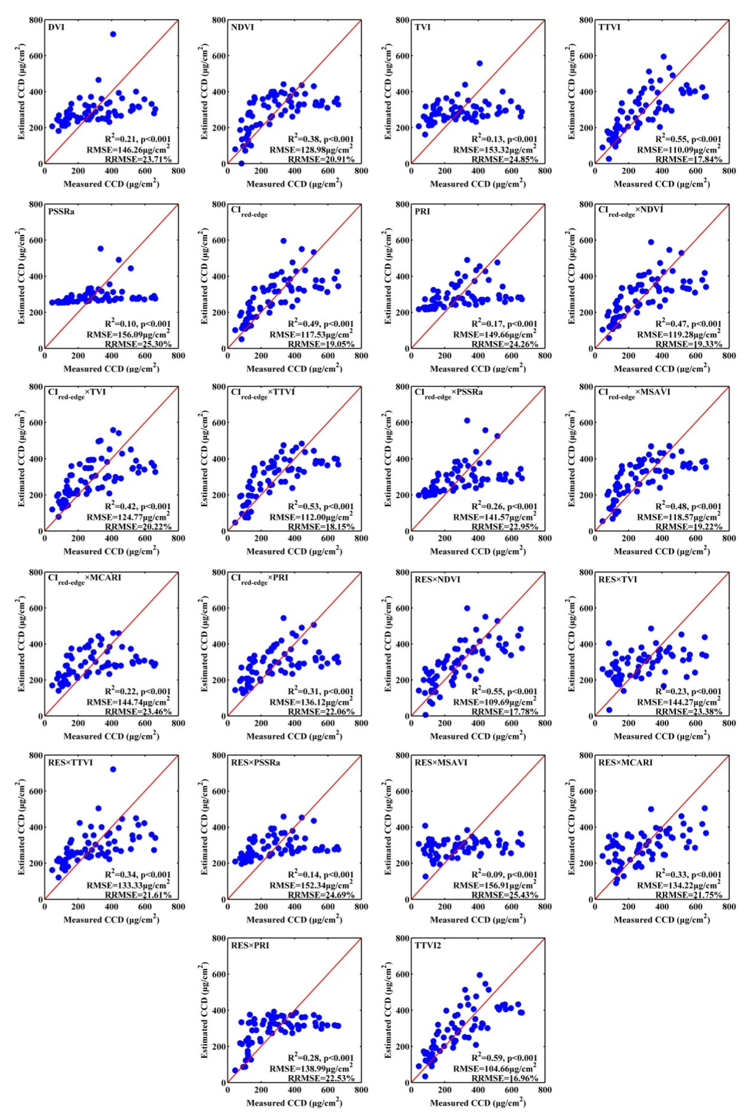
To further discover the VIs’ estimating performances, the estimation results of all the indices at different growth stages were analyzed in the study. To maximize the usage of limited datasets, k-fold cross-validation (k = 4) was used for parameter estimation. Based on the estimation models from Section 3.1, the estimation of the LAI and CCD values at four growth stages was conducted. The estimating indicators, including R2, RMSE, and RRMSE, are shown in Table 4 and Figure 6.
As seen from Figure 6, the estimation for LAI was distinct at different growth stages. For the early jointing stage, the indices exhibited poor performances, with R2 values reaching no more than 0.1. There was almost no correlation between indices and LAI, indicating that they might be unable to assess winter wheat LAI at this stage. For the late jointing stage, the performances were better, with an increase in R2 values. CIred-edge and CIred-edge-integrated indices exhibited good performances and outperformed RES-integrated indices. The classical LAI-sensitive indices, DVI, NDVI, and TVI, were not good estimators at this stage. The estimation at the head emergence stage was similar to that of the last stage, with a relatively higher R2. The estimation at the filling stage was no better than that at the late jointing stage and head emergence stage. However, it was still better than that at the early jointing stage.
The variation trend of R2 values of LAI retrieval started with a smaller value at the early jointing stage, increased to a higher value at the late jointing stage and head emergence stage, and finally decreased at the filling stage. This trend also applied to the CCD estimation. As seen from Figure 6, the indices exhibited the worst performances at the early jointing stage but showed better estimation at the late jointing stage and head emergence stage. There was a decrease in R2 values at the filling stage, but they still outperformed the early jointing stage. CIred-edge-integrated indices were better for CCD estimation at the head emergence stage, with comparatively higher R2 values and lower RRMSE values. These results are consistent with the research of previous studies and can be concluded as indicating the sensitivity of canopy reflectance against LAI and CCD [56]. When LAI increased, the NIR reflectance increased but the red reflectance decreased at the early growth stages, and then reached the asymptote as LAI exceeded three [56].
TTVI2 might not be the best estimation index for all growth stages. However, TTVI2 excelled far beyond the other indices with its ability to estimate the LAI and CCD at four stages, especially for the head emergence stage and filling stage. Several indices used in this research, such as CIred-edge×PRI and CIred-edge×PSSRa, performed good estimations for CCD at the late jointing stage, with R2 values greater than 0.5, but the estimations for other growth stages were poor. Another example is RES×TTVI. The index had the highest R2 value at the filling stage of 0.41 and the lowest RRMSE of 19.87%; however, the estimations at the other stages were not acceptable.

3.3. Validation

A total of 22 hyperspectral indices were validated in this section, including: DVI, NDVI, TVI, TTVI, PSSRa, CIred-edge, PRI; integration-based indices CIred-edge×NDVI, CIred-edge×TVI, CIred-edge×TTVI, CIred-edge×PSSRa, CIred-edge×MSAVI, CIred-edge×MCARI, CIred-edge×PRI, RES×NDVI, RES×TVI, RES×TTVI, RES×PSSRa, RES×MSAVI, RES×MCARI, and RES×PRI; and the newly proposed TTVI2 index. The results are shown in Figure 7 and Figure 8. The estimation models from Section 3.1 were further applied to hyperspectral indices for LAI and CCD estimations. The validation process was conducted against field-measured LAI, CCD, and hyperspectral-estimated parameters pooled at four stages. The estimations were calculated from those in PROSAIL models. The validation results may differ from the estimation results for some of the indices. Analyzing and comparing the joint retrieval ability was the research object in this study. Thus, R2, RMSE, and RRMSE were used as indicators for evaluating estimations. The comparison of RRMSE helps us analyze the performances not only from the single model of the specific index but also as a comparison among all the indices. A lower RMSE and RRMSE indicate a better predictor for the parameters.
Generally, the majority of vegetation indices presented reliable estimates for LAI, with acceptable R2 and RMSE values. TTVI2 exhibited a significant linear trend with winter wheat LAI. The scatterplots plotted closer to the 1:1 line, compared with other indices. It also performed the best estimation, with the highest R2 value of 0.76 and lowest RMSE and RRMSE values of 0.93 m2/m2 and 12.76%, respectively. TTVI, CIred-edge×TTVI, and RES×TTVI also exhibit good performances. Only the RRMSE reveals that their estimations were not as good as that of TTVI2. Classical vegetation indices, including DVI and NDVI, are still good for LAI retrieval, but the saturation effect hinders the estimation for an LAI greater than 6. The CIred-edge-integrated indices estimated the LAI with fairly equal R2 values. The CIred edge might play a dominant role in the integrations. The success of CIred-edge integrations also reflects the merits of reciprocal data in parameter retrieval.
For CCD retrieval, the overall estimation was not as good as that of LAI, as seen from the corresponding RRMSE. The underestimation was obvious for CIred-edge-integrated and RES-integrated indices. TTVI2 still showed the best performance for CCD, with the highest R2 value of 0.59 and lowest RMSE and RRMSE of 104.66 μg/cm2 and 16.96%, respectively. The scatterplot pattern is similar for TTVI2 and TTVI, considering their analogous formulations. PSSRa exhibited a moderate performance for LAI but was almost resistant to CCD variations. RES×NDVI was rather scattered while estimating CCD.
For the joint retrieval of LAI and CCD, some indices yielded unexpected results. PRI was supposed to be related to both LAI and CCD, but the plots were scattered with relatively low R2 values. We cannot deny the estimation ability of PRI. The reason might be that the index is not suitable for winter wheat. Its combination with CIred-edge was slightly better but was not suitable for joint retrieval. The saturation effect might be an obstacle for this index. TTVI2, TTVI, CIred-edge×TTVI, and RES×NDVI can be considered good indices for the simultaneous retrieval of LAI and CCD. RES×NDVI did not perform well with the POSAIL dataset but was good with field-measured data. However, the multiplication of LAI-sensitive and CCD-sensitive indices was not always successful. The combination with CIred-edge was better than those with RES. There was an underestimation of RES-integrated indices under high CCD and LAI values. RES×MSAVI exhibited poor estimation for both LAI and CCD, with an R2 value no higher than 0.1, which was consistent with the estimation results in Section 3.1.
A key point in this research is that the retrieval of pooled LAI and CCD is better than the retrieval at different growth stages with higher R2 values.

4. Discussion

Integration-based indices and the new index TTVI2 are proposed in this study for LAI and CCD joint retrieval. Compared with published indices, part of the integration-based indices and TTVI2 are able to predict both the LAI and CCD of winter wheat. The development of the new index improves the calculation efficiency, which enables us to acquire both biophysical and biochemical data through a simple process. It simplifies the processes of selecting and calculating optimal indices. There might be a debate on whether a single index is able to estimate the LAI and CCD simultaneously. This consideration might focus on the overlapping sensitive spectral regions for biophysical and biochemical parameters. However, in this study, we avoid overlapped regions and utilize spectral regions that are sensitive to both parameters. The concept of integrating published vegetation indices to exploit their expanding application is demonstrated as being useful to some extent. The research basis of the joint retrieval of LAI and CCD lies in the dynamic variation at growth stages, due to winter wheat characteristics. The parameters have an effect on each other. The increase in the leaf area offers an opportunity for more chloroplast formation. In response, a higher chlorophyll content leads to greater vigor in photosynthesis and produces more leaves. Therefore, not only the individual parameters but also the overall situation matter.
Even though the two methods worked for the joint retrieval of LAI and CCD, some key points need to be noted. The multiplication of a LAI-sensitive index and a chlorophyll-sensitive index is not a prerequisite of a CCD-sensitive index. In contrast, a CCD-sensitive index might not be sensitive to its composition in LAI or LCD. The sensitive wavelengths and forms used in the index are what matter. For example, RES is a good predictor of chlorophyll content, and MSAVI is linearly related to the green LAI [25,33]. However, the RES-integrated and MSAVI-integrated indices don’t show good estimations for LAI or CCD. The reason might lie in that MSAVI was designed to minimize the effect of chlorophyll content on the prediction of green LAI with a self-adjustment factor [25]. It is a good LAI estimator that is less affected by canopy parameters, thus it is apparently very resistant to chlorophyll [57]. There is the possibility that the integration takes advantage of both sides, but there is also the possibility that the multiplications cause more problems than before. Taking TTVI as an example, the integrated index CIred-edge×TTVI is not as good as TTVI itself. Even for the same index CIred-edge, its combination with TTVI performed well in estimation, but its integration with PSSRa was poor when performing parameter retrieval. In conclusion, the selection of indices is important. If one of the indices is resistant to another, the multiplication of the two indices will do harm instead of supporting retrieval.
In addition, the estimation results and validation results can be inconsistent for some indices. Backtracking the processes, the only difference lies in the datasets. The PROSAIL dataset was used to establish models, and validation was conducted against a field-measured hyperspectral dataset. Good results of an index observed on both field measured data and simulated dataset would indicate that this index is in agreement with field measurements and could potentially be applied to a wide range of crop species. Good results for simulated datasets, but poor results for field datasets, indicate that the index is limited to specific species or crops. The opposite situation, where an index is good for field datasets but gives poor results for simulated datasets, demonstrates that the simulated dataset might not be able to represent the specified crop [58].
Another finding in this research is that REIP is not linearly related to the variation of CCD and LAI. In addition, the relationship is not fixed. The red edge shifted faster toward longer wavelengths with increasing chlorophyll contents ranging from 100 to 300 μg/cm2, and the movement of the red edge position slowed down even when the chlorophyll content was greater than 300 μg/cm2. This explains why some of the indices could be sensitive to parameters, while others were not correlated to vegetation parameters. The longest red-edge inflection point in this study is 740 nm. According to the relationships between the red-edge shift wavelengths and LAI/CCD, the red-edge-based indices can better estimate the parameters at the beginning of the crop growth stages, when LAI and CCD increase slowly, and the values are not very high. This might be useful to explain why a massive number of indices exhibited exponential or multiple relationships with vegetation parameters.
In addition, the sensitivities of TTVI2 to interfering factors like soil background, atmospheric conditions, BRDF effects, and surface topography need to be discussed. The topographic effect can bring noise to LAI retrieval, especially for hilly areas [59,60]. According to a previous study, the topographic effect can be reduced by band ratios, due to the spectrum similarity between NIR and visible bands [61]. In this study, the TTVI2 was only used for a row crop—winter wheat, and the experimental area is in plain terrain. The influence of surface topography, or the difference in solar radiation between a sunny (equatorial-facing) slope and shady (polar-facing) slope, is inconspicuous. The research of its sensitivity to topographical effect can be tested on heterogeneous terrain in the future. Besides this, the field hyperspectral spectrum was collected at a height of 1.3 m above the ground. The observing range is about 1 m2, with winter wheat taking up the major view. Thus, the BRDF effect might not be an overwhelming interfering effect. In the study, the TTVI2 estimation models were established with simulated data and field-level hyperspectral data. Comparing this to satellite data, the scattering and absorption by atmospheric aerosols and gases can be eliminated [62]. However, the index might be used with airborne hyperspectral data like PRISMA, EO-1 Hyperion, PROBA, and GF-5 for further study, and the usage of TTVI2 can be explored. In summary, the application of TTVI2 can be further studied from the aspect of rough surface topography and its resistance to atmospheric effect. The TTVI2 is also winter wheat-specific; its suitability for other crops needs to be studied further.

5. Conclusions

We proposed two methods for the joint retrieval of winter wheat LAI and CCD in this study. The two methods both realize the joint retrieval but are successful to different extents. The first method integrated LAI-sensitive and CCD-sensitive indices to generate a new index, and the second method created a novel vegetation index incorporating sensitive wavelengths. The results indicate that both methods are feasible for joint retrieval. Only the selection of indices is complicated for the first method because not all combinations are suitable for joint retrieval. Our newly created index, i.e., the transformed triangular vegetation index (TTVI2), exhibited the highest R2 of 0.76 and 0.59 for LAI and CCD prediction, respectively. It also exhibited the lowest RMSE (0.93 m2/m2 for LAI, 104.66 μg/cm2 for CCD), and RRMSE (12.76% for LAI, 16.96% for CCD), which indicates that the estimating errors are small among all the indices. TTVI, CIred-edge×TTVI, and RES×TTVI were also good predictors for LAI and CCD. Most RES-integrated indices were poor at retrieval, which finding indicates that the selection of indices is vital for simultaneous retrieval.
The use of the new index as a proxy for plant biophysical and physiological status is convenient for remote sensing monitoring. The findings of this research exploit the application of existing vegetation indices and improve retrieval efficiency. It provides technical support in winter wheat crop growth monitoring in precision agriculture. Notably, the integration-based indices, TTVI2, and the derived conclusions in this study are specific for winter wheat, and they might have limited applicability for a wider range of crop species. The feasibility of TTVI2 in rough terrain and its extension to more crop and vegetation types needs to be researched further.

Author Contributions

Conceptualization, N.X. and W.H.; methodology, Q.X.; validation and formal analysis, N.X.; writing the original draft, review and editing, N.X.; supervision, Y.R. and H.Y.; funding acquisition, W.H. All authors have read and agreed to the published version of the manuscript.

Funding

This research was funded by the Strategic Priority Research Program of the Chinese Academy of Sciences (XDA19080304), National Natural Science Foundation of China (42071320, 41871339), National Special Support Program for High-level Personnel Recruitment (Wenjiang Huang), Youth Innovation Promotion Association CAS (2021119) and Future Star Talent Program of the Aerospace Information Research Institute, Chinese Academy of Sciences (2020KTYWLZX08).

Data Availability Statement

Not applicable.

Acknowledgments

The authors would like to highly appreciate the workers who conducted the experiments. Our thanks are also extended to the editors and the two reviewers for their valuable suggestions.

Conflicts of Interest

The authors declare no conflict of interest.

References

  1. Clevers, J.; Van Leeuwen, H. Combined use of optical and microwave remote sensing data for crop growth monitoring. Remote Sens. Environ. 1996, 56, 42–51. [Google Scholar] [CrossRef]
  2. Ni, J.; Zhang, J.; Wu, R.; Pang, F.; Zhu, Y. Development of an Apparatus for Crop-Growth Monitoring and Diagnosis. Sensors 2018, 18, 3129. [Google Scholar] [CrossRef] [PubMed] [Green Version]
  3. Chen, J.M.; Black, T.A. Defining leaf area index for non-flat leaves. Plant Cell Environ. 1992, 15, 421–429. [Google Scholar] [CrossRef]
  4. Bojović, B.; Marković, A. Correlation between nitrogen and chlorophyll content in wheat (Triticum aestivum L.). Kragujev. J. Sci. 2009, 31, 69–74. [Google Scholar]
  5. Schlemmer, M.; Gitelson, A.; Schepers, J.; Ferguson, R.; Peng, Y.; Shanahan, J.; Rundquist, D. Remote estimation of nitrogen and chlorophyll contents in maize at leaf and canopy levels. Int. J. Appl. Earth Obs. Geoinf. 2013, 25, 47–54. [Google Scholar] [CrossRef] [Green Version]
  6. Broge, N.; Mortensen, J. Deriving green crop area index and canopy chlorophyll density of winter wheat from spectral reflectance data. Remote Sens. Environ. 2002, 81, 45–57. [Google Scholar] [CrossRef]
  7. Son, N.T.; Chen, C.F.; Chang, L.Y.; Duc, H.N.; Nguyen, L.D. Prediction of rice crop yield using MODIS EVI−LAI data in the Mekong Delta, Vietnam. Int. J. Remote Sens. 2013, 34, 7275–7292. [Google Scholar] [CrossRef]
  8. Thenkabail, P.S.; Smith, R.B.; De Pauw, E. Hyperspectral Vegetation Indices and Their Relationships with Agricultural Crop Characteristics. Remote Sens. Environ. 2000, 71, 158–182. [Google Scholar] [CrossRef]
  9. Thenkabail, P.S.; Smith, R.B.; De Pauw, E. Evaluation of narrowband and broadband vegetation indices for determining optimal hyperspectral wavebands for agricultural crop characterization. Photogramm. Eng. Remote Sens. 2002, 68, 607–622. [Google Scholar]
  10. Baret, F.; Guyot, G. Potentials and limits of vegetation indices for LAI and APAR assessment. Remote Sens. Environ. 1991, 35, 161–173. [Google Scholar] [CrossRef]
  11. Clevers, J.G.P.W.; Kooistra, L.; van den Brande, M.M.M. Using Sentinel-2 Data for Retrieving LAI and Leaf and Canopy Chlorophyll Content of a Potato Crop. Remote Sens. 2017, 9, 405. [Google Scholar] [CrossRef] [Green Version]
  12. Delegido, J.; Verrelst, J.; Alonso, L.; Moreno, J. Evaluation of Sentinel-2 Red-Edge Bands for Empirical Estimation of Green LAI and Chlorophyll Content. Sensors 2011, 11, 7063–7081. [Google Scholar] [CrossRef] [PubMed] [Green Version]
  13. Blackburn, G.A. Quantifying chlorophylls and caroteniods at leaf and canopy scales: An evaluation of some hyperspectral approaches. Remote Sens. Environ. 1998, 66, 273–285. [Google Scholar] [CrossRef]
  14. Clevers, J.G.; Kooistra, L. Using hyperspectral remote sensing data for retrieving canopy chlorophyll and nitrogen content. IEEE J. Sel. Top. Appl. Earth Obs. Remote Sens. 2011, 5, 574–583. [Google Scholar] [CrossRef]
  15. Fang, H.; Liang, S. Retrieving leaf area index with a neural network method: Simulation and validation. IEEE Trans. Geosci. Remote Sens. 2003, 41, 2052–2062. [Google Scholar] [CrossRef] [Green Version]
  16. Li, Z.; Jin, X.; Wang, J.; Yang, G.; Nie, C.; Xu, X.; Feng, H. Estimating winter wheat (Triticum aestivum) LAI and leaf chlorophyll content from canopy reflectance data by integrating agronomic prior knowledge with the PROSAIL model. Int. J. Remote Sens. 2015, 36, 2634–2653. [Google Scholar] [CrossRef]
  17. Dong, T.; Liu, J.; Shang, J.; Qian, B.; Ma, B.; Kovacs, J.M.; Walters, D.; Jiao, X.; Geng, X.; Shi, Y. Assessment of red-edge vegetation indices for crop leaf area index estimation. Remote Sens. Environ. 2019, 222, 133–143. [Google Scholar] [CrossRef]
  18. Li, W.; Weiss, M.; Waldner, F.; Defourny, P.; Demarez, V.; Morin, D.; Hagolle, O.; Baret, F. A Generic algorithm to estimate LAI, FAPAR and FCOVER variables from SPOT4_HRVIR and landsat sensors: Evaluation of the consistency and comparison with ground measurements. Remote Sens. 2015, 7, 15494–15516. [Google Scholar] [CrossRef] [Green Version]
  19. Eriksson, H.; Eklundh, L.; Hall, K.; Lindroth, A. Estimating LAI in deciduous forest stands. Agric. For. Meteorol. 2005, 129, 27–37. [Google Scholar] [CrossRef]
  20. Kawashima, S.; Nakatani, M. An algorithm for estimating chlorophyll content in leaves using a video camera. Ann. Bot. 1998, 81, 49–54. [Google Scholar] [CrossRef] [Green Version]
  21. Gitelson A, A. Wide dynamic range vegetation index for remote quantification of biophysical characteristics of vegetation. J. Plant Physiol. 2004, 161, 165–173. [Google Scholar] [CrossRef] [Green Version]
  22. Daughtry, C.S.T.; Walthall, C.L.; Kim, M.S.; De Colstoun, E.B.; McMurtrey, J.E. Estimating Corn Leaf Chlorophyll Concentration from Leaf and Canopy Reflectance. Remote Sens. Environ. 2000, 74, 229–239. [Google Scholar] [CrossRef]
  23. Blackburn, G.A. Spectral indices for estimating photosynthetic pigment concentrations: A test using senescent tree leaves. Int. J. Remote Sens. 1998, 19, 657–675. [Google Scholar] [CrossRef]
  24. Xing, N.; Huang, W.; Xie, Q.; Shi, Y.; Ye, H.; Dong, Y.; Wu, M.; Sun, G.; Jiao, Q. A transformed triangular vegetation index for estimating winter wheat leaf area index. Remote Sens. 2020, 12, 16. [Google Scholar] [CrossRef] [Green Version]
  25. Haboudane, D.; Miller, J.R.; Pattey, E.; Zarco-Tejada, P.J.; Strachan, I.B. Hyperspectral vegetation indices and novel algorithms for predicting green LAI of crop canopies: Modeling and validation in the context of precision agriculture. Remote Sens. Environ. 2004, 90, 337–352. [Google Scholar] [CrossRef]
  26. Rondeaux, G.; Steven, M.; Baret, F. Optimization of Soil-Adjusted Vegetation Indices. Remote Sens. Environ. 1996, 55, 95–107. [Google Scholar] [CrossRef]
  27. Dash, J.; Curran, P.J. The MERIS terrestrial chlorophyll index. Int. J. Remote Sens. 2004, 25, 5403–5413. [Google Scholar] [CrossRef]
  28. Cui, B.; Zhao, Q.; Huang, W.; Song, X.; Ye, H.; Zhou, X. A new integrated vegetation index for the estimation of winter wheat leaf chlorophyll content. Remote Sens. 2019, 11, 974. [Google Scholar] [CrossRef] [Green Version]
  29. Banerjee, V.; Krishnan, P.; Das, B.; Verma, A.; Varghese, E. Crop Status Index as an indicator of wheat crop growth condition under abiotic stress situations. Field Crops Res. 2015, 181, 16–31. [Google Scholar] [CrossRef]
  30. Houborg, R.; McCabe, M.; Cescatti, A.; Gao, F.; Schull, M.; Gitelson, A. Joint leaf chlorophyll content and leaf area index retrieval from Landsat data using a regularized model inversion system (REGFLEC). Remote Sens. Environ. 2015, 159, 203–221. [Google Scholar] [CrossRef] [Green Version]
  31. Haboudane, D.; Miller, J.R.; Tremblay, N.; Zarco-Tejada, P.J.; Dextraze, L. Integrated narrow-band vegetation indices for prediction of crop chlorophyll content for application to precision agriculture. Remote Sens. Environ. 2002, 81, 416–426. [Google Scholar] [CrossRef]
  32. Delegido, J.; Verrelst, J.; Meza, C.; Rivera, J.; Alonso, L.; Moreno, J. A red-edge spectral index for remote sensing estimation of green LAI over agroecosystems. Eur. J. Agron. 2013, 46, 42–52. [Google Scholar] [CrossRef]
  33. Chang-Hua, J.; Yong-Chao, T.I.A.N.; Xia, Y.A.O.; Wei-Xing, C.A.O.; Yan, Z.H.U.; Hannaway, D. Estimating leaf chlorophyll content using red edge parameters. Pedosphere 2010, 20, 633–644. [Google Scholar]
  34. Sharma, L.K.; Bu, H.; Denton, A.; Franzen, D.W. Active-Optical Sensors Using Red NDVI Compared to Red Edge NDVI for Prediction of Corn Grain Yield in North Dakota, U.S.A. Sensors 2015, 15, 27832–27853. [Google Scholar] [CrossRef]
  35. Kanke, Y.; Tubaña, B.; Dalen, M.; Harrell, D. Evaluation of red and red-edge reflectance-based vegetation indices for rice biomass and grain yield prediction models in paddy fields. Precis. Agric. 2016, 17, 507–530. [Google Scholar] [CrossRef]
  36. Zhou, X.; Huang, W.; Kong, W.; Ye, H.; Dong, Y.; Casa, R. Assessment of leaf carotenoids content with a new carotenoid index: Development and validation on experimental and model data. Int. J. Appl. Earth Obs. Geoinf. 2017, 57, 24–35. [Google Scholar] [CrossRef]
  37. Gao, J. Experimental Guidance for Plant Physiology; China Higher Education Press: Beijing, China, 2006. [Google Scholar]
  38. Verrelst, J.; Camps-Valls, G.; Muñoz-Marí, J.; Rivera, J.P.; Veroustraete, F.; Clevers, J.; Moreno, J. Optical remote sensing and the retrieval of terrestrial vegetation bio-geophysical properties—A review. ISPRS J. Photogramm. Remote Sens. 2015, 108, 273–290. [Google Scholar] [CrossRef]
  39. Jacquemoud, S.; Verhoef, W.; Baret, F.; Bacour, C.; Zarco-Tejada, P.J.; Asner, G.P.; François, C.; Ustin, S.L. PROSPECT+SAIL models: A review of use for vegetation characterization. Remote Sens. Environ. 2009, 113, S56–S66. [Google Scholar] [CrossRef]
  40. Li, Z.; Jin, X.; Yang, G.; Drummond, J.; Yang, H.; Clark, B.; Li, Z.; Zhao, C. Remote sensing of leaf and canopy nitrogen status in winter wheat (Triticum aestivum L.) based on N-PROSAIL model. Remote Sens. 2018, 10, 1463. [Google Scholar] [CrossRef] [Green Version]
  41. Xie, Q.; Dash, J.; Huete, A.; Jiang, A.; Yin, G.; Ding, Y.; Peng, D.; Hall, C.C.; Brown, L.; Shi, Y.; et al. Retrieval of crop biophysical parameters from Sentinel-2 remote sensing imagery. Int. J. Appl. Earth Obs. Geoinf. 2019, 80, 187–195. [Google Scholar] [CrossRef]
  42. Duveiller, G.; Weiss, M.; Baret, F.; Defourny, P. Retrieving wheat Green Area Index during the growing season from optical time series measurements based on neural network radiative transfer inversion. Remote Sens. Environ. 2011, 115, 887–896. [Google Scholar] [CrossRef]
  43. Fang, H.; Baret, F.; Plummer, S.; Schaepman-Strub, G. An overview of global leaf area index (LAI): Methods, products, validation, and applications. Rev. Geophys. 2019, 57, 739–799. [Google Scholar] [CrossRef]
  44. Xie, Q.; Huang, W.; Zhang, B.; Chen, P.; Song, X.; Pascucci, S.; Pignatti, S.; Laneve, G.; Dong, Y. Estimating Winter Wheat Leaf Area Index From Ground and Hyperspectral Observations Using Vegetation Indices. IEEE J. Sel. Top. Appl. Earth Obs. Remote Sens. 2015, 9, 771–780. [Google Scholar] [CrossRef]
  45. Gitelson, A.A.; Gritz, Y.; Merzlyak, M.N. Relationships between leaf chlorophyll content and spectral reflectance and algorithms for non-destructive chlorophyll assessment in higher plant leaves. J. Plant Physiol. 2003, 160, 271–282. [Google Scholar] [CrossRef]
  46. Babar, M.A.; Reynolds, M.P.; Van Ginkel, M.; Klatt, A.R.; Raun, W.; Stone, M.L. Spectral Reflectance to Estimate Genetic Variation for In-Season Biomass, Leaf Chlorophyll, and Canopy Temperature in Wheat. Crop Sci. 2006, 46, 1046–1057. [Google Scholar] [CrossRef]
  47. Gitelson, A.A.; Keydan, G.P.; Merzlyak, M.N. Three-band model for noninvasive estimation of chlorophyll, carotenoids, and anthocyanin contents in higher plant leaves. Geophys. Res. Lett. 2006, 33, L11402. [Google Scholar] [CrossRef] [Green Version]
  48. Gitelson, A.A.; Viña, A.; Ciganda, V.; Rundquist, D.C.; Arkebauer, T.J. Remote estimation of canopy chlorophyll content in crops. Geophys. Res. Lett. 2005, 32, L08403. [Google Scholar] [CrossRef] [Green Version]
  49. Wu, C.; Niu, Z.; Tang, Q.; Huang, W. Estimating chlorophyll content from hyperspectral vegetation indices: Modeling and validation. Agric. For. Meteorol. 2008, 148, 1230–1241. [Google Scholar] [CrossRef]
  50. Gamon, J.A.; Surfus, L.S.S. The Photochemical Reflectance Index: An Optical Indicator of Photosynthetic Radiation Use Efficiency across Species, Functional Types, and Nutrient Levels. Oecologia 1997, 112, 492–501. [Google Scholar] [CrossRef]
  51. Gitelson, A.A.; Gamon, J.A.; Solovchenko, A. Multiple drivers of seasonal change in PRI: Implications for photosynthesis 2. Stand level. Remote Sens. Environ. 2017, 190, 198–206. [Google Scholar] [CrossRef] [Green Version]
  52. Tucker, C.J. Red and photographic infrared linear combinations for monitoring vegetation. Remote Sens. Environ. 1979, 8, 127–150. [Google Scholar] [CrossRef] [Green Version]
  53. Clevers, J.G.; De Jong, S.; Epema, G.F.; van der Meer, F.; Bakker, W.H.; Skidmore, A.; Addink, E. MERIS and the red-edge position. Int. J. Appl. Earth Obs. Geoinf. 2001, 3, 313–320. [Google Scholar] [CrossRef]
  54. Lay, D.C.; Lay, S.R.; McDonald, J.J. Linear Algebra and Its Applications; Pearson: London, UK, 2016. [Google Scholar]
  55. Malenovský, Z.; Homolová, L.; Zurita-Milla, R.; Lukeš, P.; Kaplan, V.; Hanuš, J.; Gastellu-Etchegorry, J.P.; Schaepman, M.E. Retrieval of spruce leaf chlorophyll content from airborne image data using continuum removal and radiative transfer. Remote Sens. Environ. 2013, 131, 85–102. [Google Scholar] [CrossRef] [Green Version]
  56. Xie, Q.; Dash, J.; Huang, W.; Peng, D.; Qin, Q.; Mortimer, H.; Casa, R.; Pignatti, S.; Laneve, G.; Pascucci, S.; et al. Vegetation Indices Combining the Red and Red-Edge Spectral Information for Leaf Area Index Retrieval. IEEE J. Sel. Top. Appl. Earth Obs. Remote Sens. 2018, 11, 1482–1493. [Google Scholar] [CrossRef] [Green Version]
  57. Broge, N.H.; Leblanc, E. Comparing prediction power and stability of broadband and hyperspectral vegetation indices for estimation of green leaf area index and canopy chlorophyll density. Remote Sens. Environ. 2001, 76, 156–172. [Google Scholar] [CrossRef]
  58. Le Maire, G.; François, C.; Dufrêne, E. Towards universal broad leaf chlorophyll indices using PROSPECT simulated database and hyperspectral reflectance measurements. Remote Sens. Environ. 2004, 89, 1–28. [Google Scholar] [CrossRef]
  59. Hao, D.; Wen, J.; Xiao, Q.; Wu, S.; Lin, X.; You, D.; Tang, Y. Modeling Anisotropic Reflectance Over Composite Sloping Terrain. IEEE Trans. Geosci. Remote Sens. 2018, 56, 3903–3923. [Google Scholar] [CrossRef]
  60. Kumari, N.; Saco, P.M.; Rodriguez, J.F.; Johnstone, S.A.; Srivastava, A.; Chun, K.P.; Yetemen, O. The Grass Is Not Always Greener on the Other Side: Seasonal Reversal of Vegetation Greenness in Aspect-Driven Semiarid Ecosystems. Geophys. Res. Lett. 2020, 47, e2020GL088918. [Google Scholar] [CrossRef]
  61. Matsushita, B.; Yang, W.; Chen, J.; Onda, Y.; Qiu, G. Sensitivity of the Enhanced Vegetation Index (EVI) and Normalized Difference Vegetation Index (NDVI) to Topographic Effects: A Case Study in High-density Cypress Forest. Sensors 2007, 7, 2636–2651. [Google Scholar] [CrossRef] [Green Version]
  62. Kaufman, Y.; Tanre, D. Atmospherically resistant vegetation index (ARVI) for EOS-MODIS. IEEE Trans. Geosci. Remote Sens. 1992, 30, 261–270. [Google Scholar] [CrossRef]
Figure 1. Study sites and the distribution of sampling points in Beijing, Shunyi District. The satellite background is the border of the Shunyi district. (ad) are photos of sampling points No. 20, No. 16, No. 9, and No. 4 at the early jointing stage.
Remotesensing 13 03175 g001
Figure 2. The Pearson correlation coefficient between simulated spectral reflectance and vegetation parameters.
Remotesensing 13 03175 g002
Figure 3. The relationship between the red-edge position and canopy chlorophyll density.
Remotesensing 13 03175 g003
Figure 4. The correlation between TVI-like indices and vegetation parameters. (a) Correlation between the LAI and wavelengths, (b) correlation between the CCD and wavelengths.
Remotesensing 13 03175 g004
Figure 5. The triangular area of the transformed triangular vegetation index 2 (TTVI2). The vegetation reflectance comes from the No. 9 sampling plot at the head emergence stage.
Remotesensing 13 03175 g005
Figure 6. The estimation results for LAI and CCD at different growth stages. Figures (a,c,e) show the R2, RSMSE, and RRMSE results between VIs and LAI; (b,d,f) are the corresponding results between VIs and CCD.
Remotesensing 13 03175 g006
Figure 7. Scatterplots of the measured LAI versus estimated LAI, derived from ground hyperspectral vegetation indices. Red dashed lines indicate the 1:1 line.
Remotesensing 13 03175 g007
Figure 8. Scatterplots of the measured CCD versus the estimated CCD derived from ground hyperspectral vegetation indices. Red solid lines indicate 1:1 lines.
Remotesensing 13 03175 g008
Table 1. Sample plots at four growth stages.
Growth Stages.Total Sample PlotsSelected Sample Plots
Early jointing stage2418
Late jointing stage2418
Head emergence stage2418
Filling stage2418
Pooled9672
Table 2. Input parameter settings in the PROSAIL model.
ParametersNotesValueDistributionUnitsNumber
Leaf parameters
NLeaf structure parameter1.3Gaussian-1
CwWater content0.01 cm1
CmDry matter content0.004 g/cm21
CabChlorophyll a + b content12.96~113.16Gaussian standard deviation of 50, mean value of 50μg/cm230
Canopy parameters
LAILeaf area index0.5~8.5Uniformm2/m230
ALAAverage leaf angle30,45 degree2
hotHot spot parameter0.12~0.21Uniformm/m3
θsSolar zenith angle35 1
Table 3. List of vegetation indices used in the study. All the indices were calculated with hyperspectral resolution data in this study.
IndexDescriptionCalculationRelated toReference
DVIDifference vegetation index R 800 R 680 LAI[52]
NDVINormalized difference vegetation index ( R 800 R 680 ) / ( R 800 + R 680 ) LAI[23]
TVITriangular vegetation index 0.5 × [ 120 × ( R 750 R 550 ) 200 × ( R 670 R 550 ) ] LAI[25]
TTVITransformed triangular vegetation index 0.5 × [ ( 783 740 ) × ( R 865 R 740 ) ( 865 740 ) × ( R 783 R 740 ) ] LAI[24]
PSSRaPigment-specific simple ratio R 800 / R 680 CCD[13]
CIred-edgeRed-edge chlorophyll index ( R 780 / R 710 ) 1 CCD[45,47]
RESRed edge symmetry ( R 718 R 675 ) / ( R 755 R 675 ) CCD[33]
PRIPhotochemical reflectance index ( R 531 R 570 ) / ( R 531 + R 570 ) LAI, CCD[50]
MCARIModified chlorophyll absorption ratio index [ ( R 700 R 670 ) 0.2 × ( R 700 R 550 ) ] ( R 700 / R 670 ) CCD[25]
MSAVIModified soil-adjusted vegetation index 0.5 × [ 2 R 800 + 1 ( 2 R 800 + 1 ) 2 8 ( R 800 R 670 ) ] LAI[25]
Table 4. The best-fit models for PROSAIL-derived indices and vegetation parameters.
Vegetation IndicesEquationsR2
Indices sensitive to LAIDVILAI = 17.359x − 3.2295R2 = 0.77
CCD = 13.805exp(5.6679x)R2 = 0.61
NDVILAI = 0.0508exp(4.9621x)R2 = 0.84
CCD = 1.7412exp(5.3067x)R2 = 0.66
TVILAI = 0.4118exp(0.0936x)R2 = 0.73
CCD = 29.572exp(0.0735x)R2 = 0.31
TTVILAI = 0.7212x + 0.8171R2 = 0.64
CCD = 58.487x − 57.855R2 = 0.93
Indices sensitive to chlorophyll contentPSSRaLAI = 0.1895x + 0.3459R2 = 0.84
CCD = 39.318exp(0.068x)R2 = 0.78
CIred-edgeLAI = 2.2074ln(x) + 1.809R2 = 0.45
CCD = 65.064x − 22.27R2 = 0.91
Indices for joint retrievalPRILAI = 1.5749exp(59.885x)R2 = 0.97
CCD = 72.208exp(59.885x)R2 = 0.67
CIred-edge×NDVILAI = 1.9344ln(x) + 2.4569R2 = 0.51
CCD = 66.614x − 3.4656R2 = 0.92
CIred-edge×TVILAI = 1.9757ln(x) − 3.978R2 = 0.62
CCD = 2.5883x − 8.544R2 = 0.93
CIred-edge×TTVILAI = 1.2541ln(x) + 1.1513R2 = 0.55
CCD = 6.2787x + 72.157R2 = 0.93
CIred-edge×PSSRaLAI = 1.3206ln(x) − 0.8848R2 = 0.66
CCD = 1.735x + 52.04R2 = 0.94
CIred-edge×MSAVILAI = 1.8228ln(x) + 2.9543R2 = 0.58
CCD = 72.364x + 10.192R2 = 0.94
CIred-edge×MCARILAI= 1.5191ln(x) + 7.1729R2 = 0.48
CCD = 123.48exp(0.9887x)R2 = 0.04
CIred-edge×PRILAI = 9.6612x + 2.5863R2 = 0.68
CCD = 683.65x + 101.39R2 = 0.75
RES×NDVILAI = −0.657ln(x) + 3.3084R2 = 0.01
CCD = −354.9ln(x) − 225.45R2 = 0.38
RES×TVILAI = 2.0488exp(0.0589x)R2 = 0.08
CCD = −123.5ln(x) + 458.13R2 = 0.10
RES×TTVILAI = 0.5659exp(1.225x)R2 = 0.85
CCD = 21.232exp(1.364x)R2 = 0.72
RES×PSSRaLAI = 0.9024exp(0.1997x)R2 = 0.78
CCD = 54.284exp(0.158x)R2 = 0.34
RES×MSAVILAI = 1.3865exp(3.5257x)R2 = 0.14
CCD = −542.55x + 343.47R2 = 0.07
RES×MCARILAI = 3.0636exp(2.0307x)R2 = 0.02
CCD = −62.16ln(x) − 45.108R2 = 0.29
RES×PRILAI = 2.666exp(31.215x)R2 = 0.79
CCD = 126.79exp(25.946x)R2 = 0.37
TTVI2LAI = 0.6796x + 0.8802R2 = 0.63
CCD = 55.897x − 56.483R2 = 0.95
1 x indicates the corresponding index. All the R2 values passed the t-test, with a p-value of less than 0.001.
Publisher’s Note: MDPI stays neutral with regard to jurisdictional claims in published maps and institutional affiliations.

