
Hyperspectral and Multispectral Image Fusion by Deep Neural Network in a Self-Supervised Manner


1
School of Geodesy and Geomatics, Wuhan University, Wuhan 430072, China
2
School of Resource and Environmental Sciences, Wuhan University, Wuhan 430072, China
*
Author to whom correspondence should be addressed.
Remote Sens. 2021, 13(16), 3226; https://0-doi-org.brum.beds.ac.uk/10.3390/rs13163226
Submission received: 18 July 2021
/
Revised: 9 August 2021
/
Accepted: 9 August 2021
/
Published: 13 August 2021
(This article belongs to the Special Issue Recent Advances in Hyperspectral Image Processing)
Abstract
:Compared with multispectral sensors, hyperspectral sensors obtain images with high- spectral resolution at the cost of spatial resolution, which constrains the further and precise application of hyperspectral images. An intelligent idea to obtain high-resolution hyperspectral images is hyperspectral and multispectral image fusion. In recent years, many studies have found that deep learning-based fusion methods outperform the traditional fusion methods due to the strong non-linear fitting ability of convolution neural network. However, the function of deep learning-based methods heavily depends on the size and quality of training dataset, constraining the application of deep learning under the situation where training dataset is not available or of low quality. In this paper, we introduce a novel fusion method, which operates in a self-supervised manner, to the task of hyperspectral and multispectral image fusion without training datasets. Our method proposes two constraints constructed by low-resolution hyperspectral images and fake high-resolution hyperspectral images obtained from a simple diffusion method. Several simulation and real-data experiments are conducted with several popular remote sensing hyperspectral data under the condition where training datasets are unavailable. Quantitative and qualitative results indicate that the proposed method outperforms those traditional methods by a large extent.
1. Introduction
Different from multispectral remote sensing images, hyperspectral remote sensing images can reflect not only the color information but also the physical property of ground objects, which contributes a lot to Earth observation tasks such as ground object classification [1], target tracking [2] and environment monitoring [3,4,5]. However, due to the signal-to-noise ratio, spatial resolution of hyperspectral images cannot be as high as that of multispectral images. The low resolution constrains the precise application of hyperspectral images. One mainstream strategy to obtain high-resolution hyperspectral (HR HSI) optical images is to fuse the spectral information from low-resolution hyperspectral (LR HSI) images and spatial information from corresponding multispectral images (HR MSI). According to the study in [6], traditional LR HSI and HR MSI fusion methods can be roughly classified into three families: (1) component substitution-based methods (CS-based methods) [7,8,9,10]; (2) multiresolution analysis-based methods (MRA-based methods) [11,12,13,14]; (3) variation model-based methods (VM-based methods) [15,16,17,18,19,20].
CS-based methods are the most traditional LR HSI and HR MSI fusion methods. They actually extend the application of CS-based methods on the pansharpening task to LR HSI and HR MSI fusion tasks. CS-based methods share the same three steps to complete the fusion process. First, they project the LR HSI to a novel feature space; then some bands in the new feature space are substituted by the bands from HR MSI. Finally, HR HSI is obtained by transforming the bands in the novel feature space back to the original space. Different projection methods contribute to different CS-based methods. These methods include Gram–Schmidt transformation (GS) [9] and Adaptive Gram–Schimidt transformation (GSA) [10]. General CS-based methods can obtain HR HSI with vivid and sharp edges. However, these transformation methods cannot obtain feature maps perfectly matching the spectral information of HR MSI. The reason is that the actual relationship between HR HSI and HR MSI is non-linear but existing transformation methods in CS-based methods are linear. Therefore, the fusion results usually have severe spectral distortion.
MRA-based methods are also most classic LR HSI and HR MSI fusion methods. They share the same main steps. First, high-frequency information and low-frequency information of LR HSI and HR MSI are separated by specific filtering methods. The fusion result is obtained by combining the high-frequency information of HR MSI and the low-frequency information of LR HSI. MRA-based methods differ from each other in terms of filtering methods. Representative filtering methods include High-pass filter (HPF) [13], Generalized Laplacian Pyramid family (GLP) [11], the decimated wavelet transform (DWT) [14] and smoothing filter-based intensity modulation (SFIM) [12]. Due to the high-frequency information having almost no spectral information, MRA-based methods avoid the effect of spectral distortion. However, the high-frequency information cannot be completely extracted by these filtering methods so MRA-based methods often suffer from the blurry spatial presentation.
VM-based methods are more novel methods than CS-based methods and MRA-based methods. They treat the fusion of LR HSI and HR MSI as an ill-posed inverse problem. Equations are first established by observation model [21,22,23] and then constrained by many handcraft priors. Popular priors contain the sparse prior [16,18,19] and low-rankness prior [24,25]. These equations are solved by iterative optimization methods such as alternating direction method of multipliers (ADMM) [26] and gradient descent algorithm [27]. Dictionary learning methods [22,23] are a representative kind of VM-based methods. By using sparse representation, they can combine the dictionaries from LR HSI and the high-resolution sparse coefficients from HR MSI to obtain HR HSI. Compared with CS-based methods and MRA-based methods, VM-based methods can acquire fusion results with better balance between spatial and spectral accuracy. However, it is hard to determine the most suitable parameters.
Due to the strong non-linear fitting ability of deep neural network, recent studies focus on introducing deep learning methods to the fusion of LR HSI and HR MSI, which can be classified as the fourth kind of methods (DL-based methods). They train the deep neural network in the supervised manner with triplets of HR HSI image, HR MSI and LR HSI image and then apply the trained network to the other data. For example, the study in [28] proposed a Unet-style network for LR HSI and HR MSI fusion tasks in order to analyze the features of multi-scales. The study in [29] took the idea from the super resolution work of 3D-CNN [30] and introduced 3D convolution layers into LR HSI and HR MSI fusion tasks. Xie, et al. [31] proposed an interpretable deep neural network for the fusion of LR HSI and HR MSI. Shuaiqi Liu, et al. [32] introduced a multi-attention-guided network and trained the network in an unsupervised manner. Lu, et al. [33] made use of a cascaded convolutional neural network for HR HSI resolution enhancement via an auxiliary panchromatic image. Despite the success of DL-based methods in LR HSI and HR MSI fusions, their performance depends heavily on the size and quality of datasets. When the dataset is small or non-existent, DL-based methods will be unsatisfying or not work. DL-based methods train the network in a supervised manner, which means they ignore the spatial and spectral features in the original resolution and have to down-sample the original HR HSI by specific times according to Wald’s protocol, largely decreasing the number of available training data. Therefore, DL-based methods are not as flexible as those traditional methods under the situation of limited dataset.
Therefore, it is of great value to explore how to obtain results by strong fitting ability of deep neural network without datasets. In some recent studies, deep neural network are introduced [34,35,36,37] to some interesting applications in a self-supervised manner where training datasets are unavailable. These applications includes style transfer [34], super-resolution and inpainting [35]. For example, given a style image and a content image, reference [34] extracts style representation of the style image and content representation of the content image from the internal layer of a pre-trained deep neural network, such as VGG19 network [38], which is a famous classification model, and combines them to optimize the input map. Finally, a style-transferred image is acquired until optimizing to the optimal. A similar work is that given a texture image, Leon Gatys, et al. [39] shows the generation of images in a VGG19 network with similar but different texture from reference image. Ulyanov, et al. [35] finds that the deep neural network itself can be viewed as a prior. With the random noise as input of network and the known degradation model, the network can complete many low-level vision tasks including super-resolution, inpainting and denoising. The above methods work well because they establish the simple yet accurate relationship between output and the given images. However, when it comes to spatial and spectral fusion tasks such as LR HSI and HR MSI fusion, they cannot extract accurate spatial and spectral features because existing methods cannot establish the complex relationship between LR HSI, HR MSI and the target image.
In order to obtain high-quality fusion results training without training datasets, we introduce a novel strategy for LR HSI and HR MSI fusion. The proposed method can operate in a self-supervised manner where all constraints in the method are constructed by LR HSI and HR MSI themselves. The process of the proposed strategy can be summarized as follows. First, the network takes a fake HR HSI as input, which is obtained roughly by a traditional information diffusion method, to obtain an initial output. Then, one optimization term is constructed between the output and LR HSI to constrain the spectral accuracy; another optimization term is constructed by the output and the fake HR HSI to constrain the spatial accuracy. By optimizing the network parameters with the two optimization terms, we obtain the final output with both high spatial and spectral accuracy. We summarize our contribution as follows:
- We introduce a strategy for self-supervised fusion of LR HSI and HR MSI. Different from deep learning methods, the proposed strategy gets rid of the dependence on the size and even the existence of a training dataset.
- A simple diffusion process is introduced as the reference to constrain the spatial accuracy of fusion results. Two simple but effective optimization terms are proposed as constraints to guarantee the spectral and spatial accuracy of fusion results.
- Several simulation and real-data experiments are conducted with some popular hyperspectral datasets. Under the condition where no training datasets are available, our method outperforms all comparison methods, testifying the superiority of the proposed strategy.
Our paper is developed with the following four sections. In Section 2, we present the workflow and the details of the proposed strategy; in Section 3, experiment results of the proposed method are displayed and compared with other state-of-the-art fusion methods under the condition without datasets. In Section 4, we discuss some findings in our experiment. In Section 5, we summarize the merits and demerits of our method applied on LR HSI and HR MSI fusions and discuss the potential improvement of the proposed method in the future.
2. Methods
2.1. Problem Formulation
Before the introduction of the proposed methods, we give some important notations for simplification and state the problem of LR HSI and HR MSI fusion. means the LR HSI image where , and are respectively the width, height and the number of channels of . is HR MSI where , and respectively mean the width, height and band number of . We aim to obtain which shares the same spatial resolution with and the same spectral resolution with . Specifically, the width and height of are much larger than those of while the channel number of is much larger than that of , i.e., , and .
It is well accepted that and are two degradation results of . On the one hand, can be viewed as the product of down-sampling by some spatial down-sampling algorithm such as bicubic and bilinear algorithm. On the other hand, is thought to be obtained by down-sampling in the spectral dimension with some spectral down-sampling algorithm . The two degradation processes are illustrated in Equations (1) and (2). The target HR HSI can be obtained by solving the Equation (3):
For the spectral degradation model , existing studies all select linear regression model or spectral response function which is also a linear model in their simulation experiments. However, the results may not be satisfying when linear spectral response function cannot accurately reflect the complex relation between and real MSI. We will reflect this phenomenon in the real experiment. We attempt to abandon and try another choice to constrain the spatial information.
2.2. Fusion Process
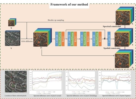
To guarantee the robustness of fusion process, we first diffuse the spatial information from to all bands of with GSA [10] to obtain a fake HR HSI as backbone:
Then serves as the input of network and we obtain an initial output from :
To constrain the spectral accuracy of , we construct the spectral optimization term directly with and :
where is the operation of down-sampling by times and is the operation of up-sampling by times. is the spatial resolution ratio between and . Although down-sampling operation can well represent the spectral information of , we add the up-sampling operation to the constraint term to further strengthen the spatial information of .
Then we make use of the to construct the spatial optimization term with to constrain the spatial accuracy of output:
With limited loss of spatial information, contains more spectral information of compared with because of the diffusion operation in Equation (4). In this way, could have less effect on the spectral accuracy of fusion results compared with .
Finally, the total optimization term, which is described in Equation (8), is constructed by the two optimization terms:
where denotes the weight.
The optimization process ends when the total optimization term reaches the optimal. Different from those deep learning-based methods whose target is a trained network, we abandon the network after optimization but retain the output:
It is worth mentioning that the whole process does not depend on a training dataset and operates in a self-supervised manner. Actually, the proposed method can also be viewed as the process of spectral information correction of .
2.3. Network Structure
We design a simple 5-layer deep neural network to complete the whole task. The whole structure and parameters are displayed in Figure 1. In each of the first five layers, there exists a convolution operation, a batch-normalization operation and a non-linear activation operation. For the last layer, there are only a convolution operation and a nonlinear activation operation. To avoid the gradient vanishing phenomena, one skip connection operations are used between the first layer and the fifth layer. Detailed parameters are listed in Figure 1.
3. Experiments
3.1. Experiment Settings
3.1.1. Datasets
We apply three hyperspectral datasets in the experiment with simulated multispectral images. They are respective CAVE dataset, Pavia University dataset and Washington DC dataset. Two datasets are used in experiment with real multispectral images. They are respectively CAVE dataset and Houston 2018 dataset. We introduce these datasets in detail.
CAVE dataset consists of 32 HR HSI, whose spatial resolution is 512 × 512. The spectral range of hyperspectral images covers from 400 nm to 700 nm and each band covers 10 nm.
Each HR HSI image has a corresponding natural RGB image with the same spatial resolution. In the experiment of CAVE dataset, we select six HR HSI images. We set the down-sampling ratio as 8 so the original HR HSI are down-sampled to 64 × 64 as the LR HSI images. For the simulation experiment, HR MSI are produced by down-sampling HR HSI images in the spectral dimension. For the real-data experiment, we make use of natural RGB images provided by the official website https://www.cs.columbia.edu/CAVE/databases/multispectral/ (accessed on 12 August 2021) of CAVE dataset.
Pavia University dataset is obtained by the Reflective Optics System Imaging Spectrometer (ROSIS) sensor. The image, whose size is 610 × 340, have the spectral range between 430 nm and 860 nm. The original image has 115 bands and only 103 bands among them are used for experiments after processing. We crop a patch with the size of 280 × 280 × 103 from the dataset as HR HSI. Then, we follow the Wald’s protocol and down-sample HR HSI by 8 times to obtain LR HSI with the size of 35 × 35 × 103. HR MSI is simulated by linearly combining the channels of HR HSI and we finally acquire HR MSI with the size of 280 × 280 × 4. In the experiment, we view HR HSI as the ground truth.
Washington DC dataset is an aerial hyperspectral image acquired by the Hydice sensor whose spectral range is between 400 nm and 2400 nm. The image has a total of 191 bands and has a size of 1208 × 307. We select a patch with the size of 280 × 280 × 191 as HR HSI and the ground truth. Then we down-sample it to the size of 35 × 35 × 191 to acquire LR HSI by following the Wald’s protocol. We also simulate HR MSI by down-sampling the HR HSI in the spectral dimension and finally obtain HR MSI with the size of 280 × 280 × 4.
Houston 2018 dataset: Houston 2018 dataset is the dataset originally used in the competition of 2018 IEEE GRSS Data Fusion. It is produced and published by University of Houston. Houston 2018 dataset consists of 14 pairs of hyperspectral images and natural HR MSI. Hyperspectral images, whose spatial resolution is 1 m, have a size of 601 × 596 and 48 bands. HR MSIs, whose spatial resolution is 0.05 m, have a size of 12,020 × 11,920 and 3 bands. In the experiment, we select 8 pairs of hyperspectral and multispectral images to testify the effectiveness of the proposed method. First, we follow the Wald’s protocol and down-sample HR MSI to the similar size of hyperspectral images. Then we crop patches with the size of 400 × 400 respectively from the hyperspectral images and the down-sampled multispectral images as the ground truth and HR MSI for fusion. The hyperspectral images are further down-sampled by 8 times to the size of 50 × 50 to get the LR HSI for fusion.
3.1.2. Comparison Methods
Different from those deep learning-based methods which need datasets for training, the proposed method needs no training datasets and can be applied on only one image in a self-supervised manner. Hence, we select six state-of-the-art fusion methods from different kinds of fusion methods. They operate under the same conditions as the comparison methods. The six selected methods are respectively Adaptive Gram-Schmidt method (GSA) [13], Coupled Nonnegative Matrix Factorization (CNMF) [17], Coupled Spectral Unmixing (ICCV15) [20], Generalized Laplacian Pyramid for HyperSharpening (GLPHS) [40], Hyperspectral Subspace regularization (HySure) [41] and Smoothing Filter-based Intensify Modulation for HyperSharpening (SFIMHS) [12].
3.1.3. Evaluation Methods
Four commonly used indexes are used to evaluate the fusion results of the proposed and the comparison methods. They are respectively peak-signal-to-noise ratio (PSNR), structure similarity index (SSIM), correlation coefficient (CC) and spectral angle mapper (SAM). The first three indexes can judge the spatial accuracy of fusion results while the last one can evaluate the spectral accuracy of fusion results. For PSNR and SSIM, a higher index means the better result. While for SAM, a lower index indicates more accurate spectral information.
3.1.4. Impletion Details
All of the experiments are conducted with Pytorch 1.0 under the environment of Ubuntu 16.04. Adam optimizer is used to optimize the fusion result and we set the learning rate of the network as 0.0002.
3.2. Experiment with Simulated Multispectral Images
In our experiment, we attempt to obtain HR HSI with spatial resolution 8 times higher than LR HSI by the process of fusion, which is a really challenging task. In this part, we test our method with images from CAVE dataset, Pavia University dataset and Washington DC dataset, with HR MSI of which are simulated by adding channels linearly from HR HSI according to the spectral response function. Linear spectral response function is also the basic assumption of the above six comparison methods.
3.2.1. CAVE Dataset
We visualize the fusion results of the proposed method and six comparison methods on CAVE dataset in Figure 2. Band 11, 21 and 31 are selected as R, G and B bands of the displayed images. Results of GSA, SFIMHS, GLPHS, CNMF are respectively displayed in Figure 2a–d. Results of ICCV15, HySure and the proposed method and the ground truth are presented in Figure 2e–h. To more intuitively compare the results of all methods, we further display their residual difference maps from the ground truth in Figure 3. It can be observed that residual map of the proposed method is darker than those of other methods, indicating that the proposed method can obtain results with least difference from the ground truth. We also compare the proposed method with the other six methods quantitatively in Table 1 which lists the three indexes mentioned above. We mark quantitative evaluation results with the highest scores in bold and those with the second highest scores with underline. The proposed method achieves the highest scores in all five indexes and outperforms the method with the second highest score by a large extent. For co-variance map and RX detection map of results in Pavia University dataset with simulated HR MSI, please view Figures S3 and S8 in Supplementary Materials.
3.2.2. Pavia University Dataset
The fusion results of patches from Pavia University dataset obtained by the seven methods are displayed in Figure 4. We select the 37th, 68th and 103rd bands as the R, G and B bands for visualization. Figure 5 presents the residual information of results from all methods compared with the ground truth. The proposed method has the less residual information in the fusion result than the other methods. We also compare the fusion results with quantitative evaluation in Table 2. The evaluation results with the highest scores are marked in bold and those with the second highest scores are marked with underline. Again the proposed method achieves the highest scores in all five evaluation indexes, indicating that the result of the proposed method is the most accurate in both spatial and spectral details. For co-variance map and RX detection map of results in Pavia University dataset with simulated HR MSI, please view Figures S6 and S11 in Supplementary Materials.
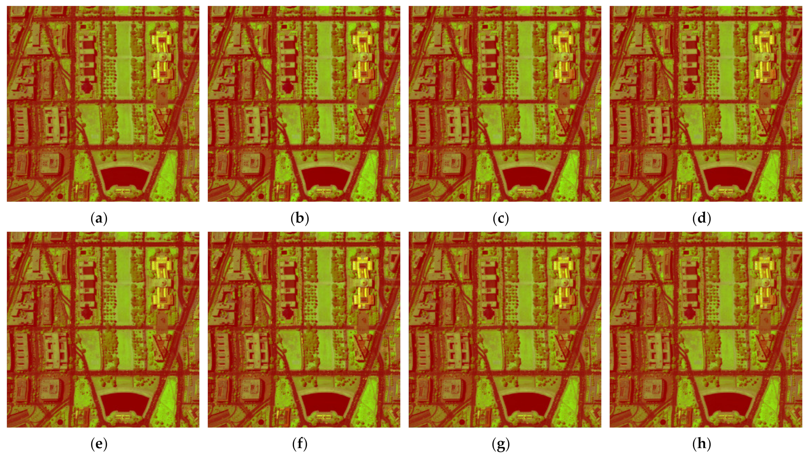
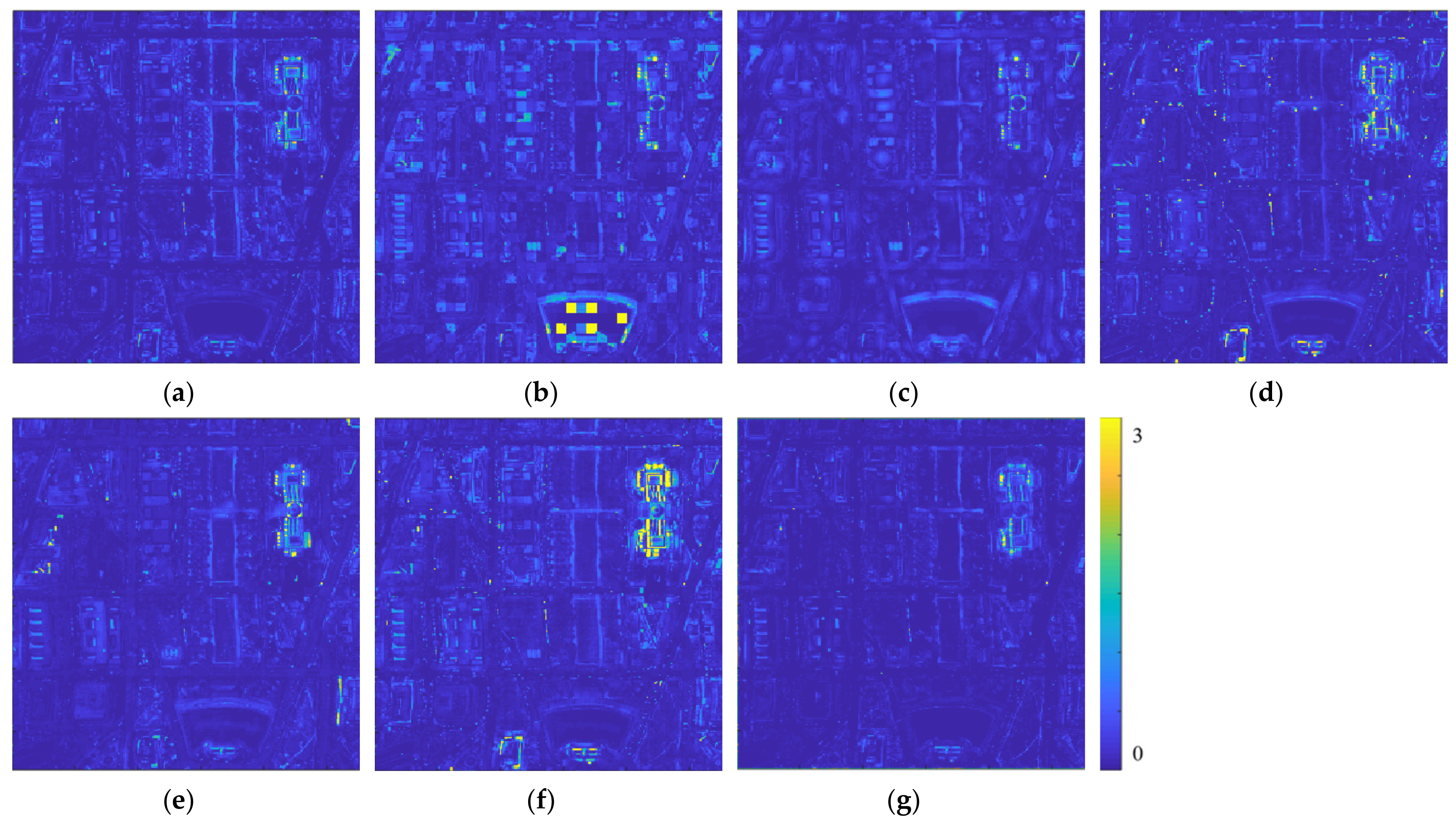
3.2.3. Washington DC Dataset
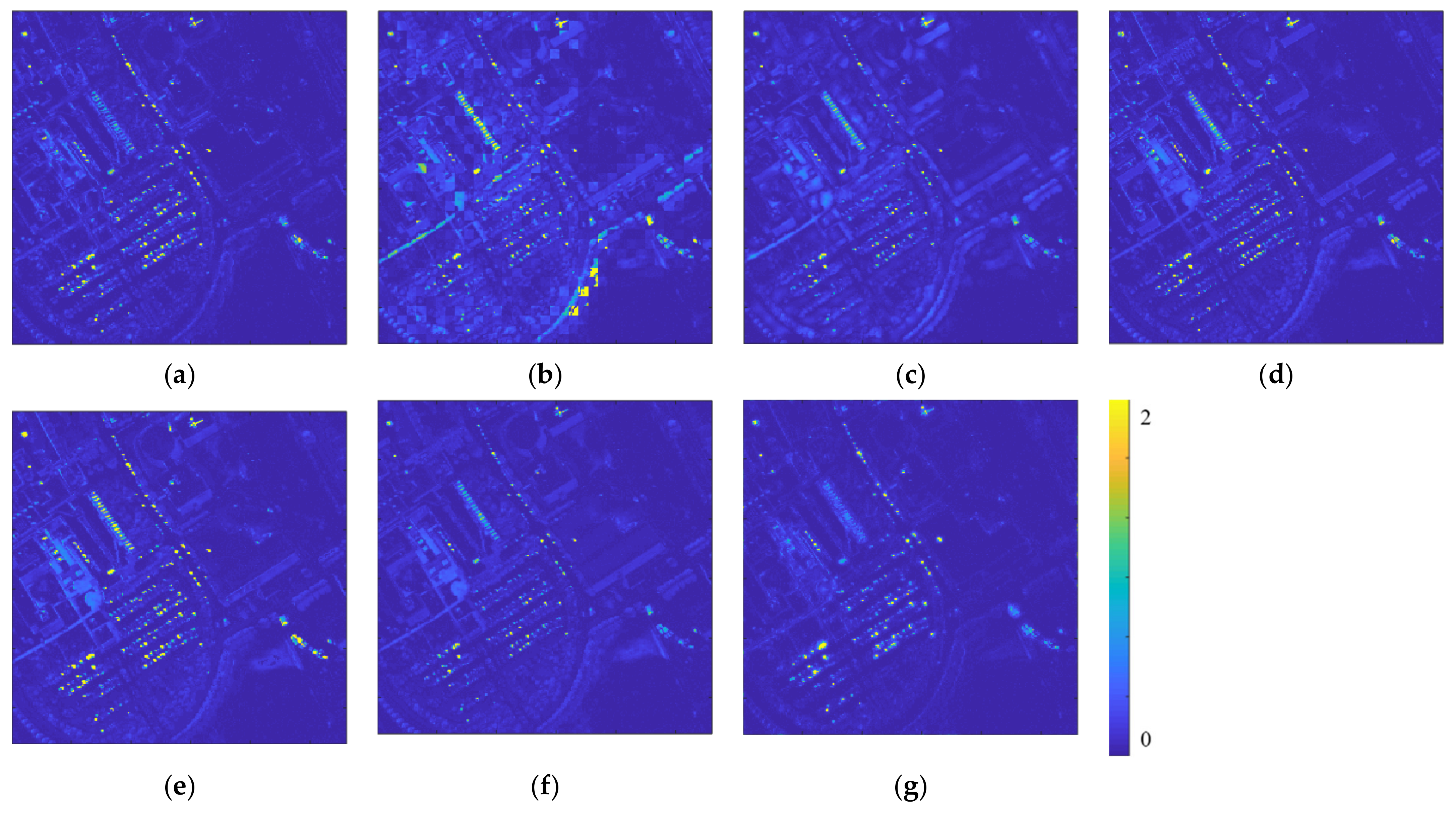
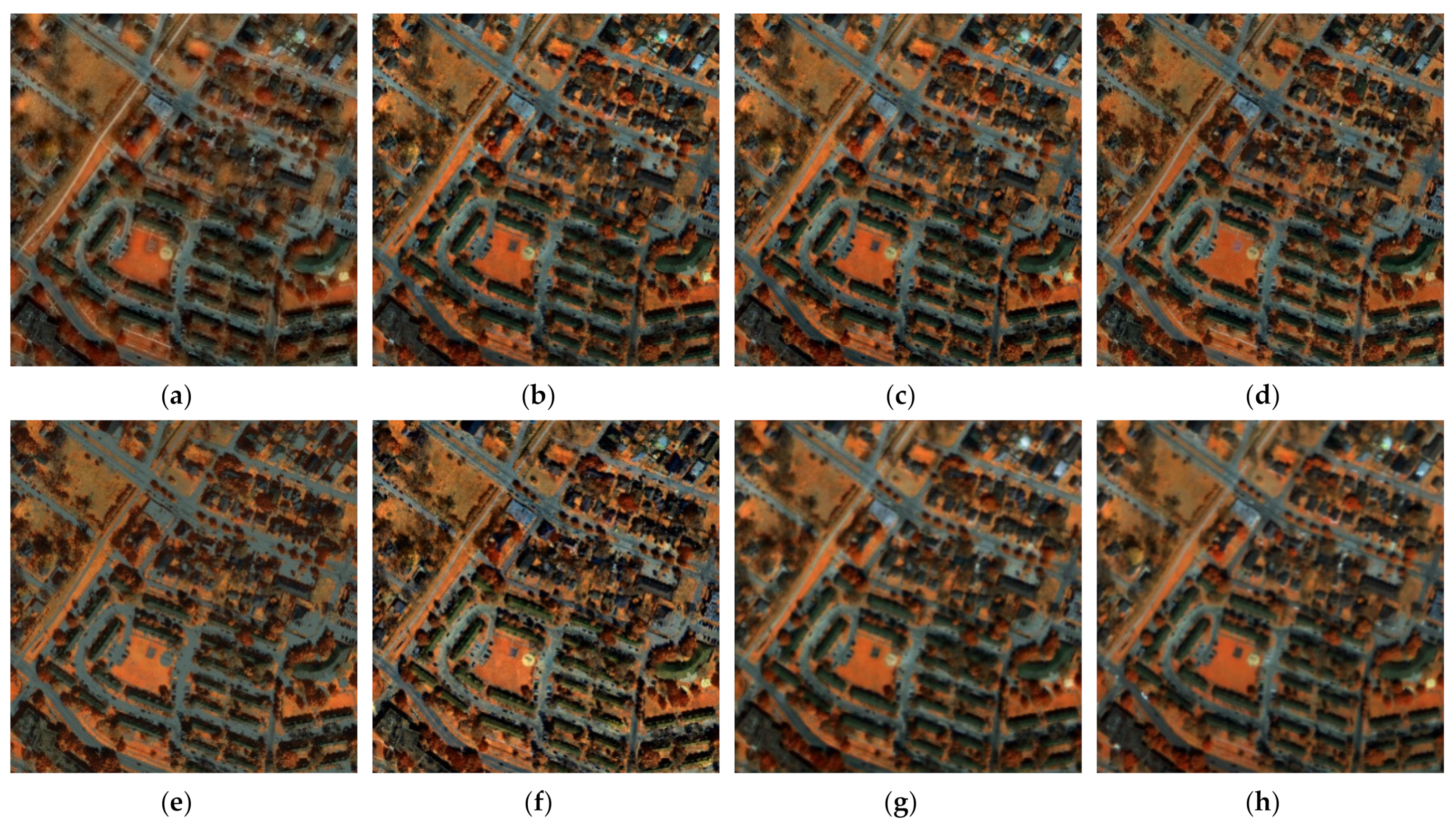
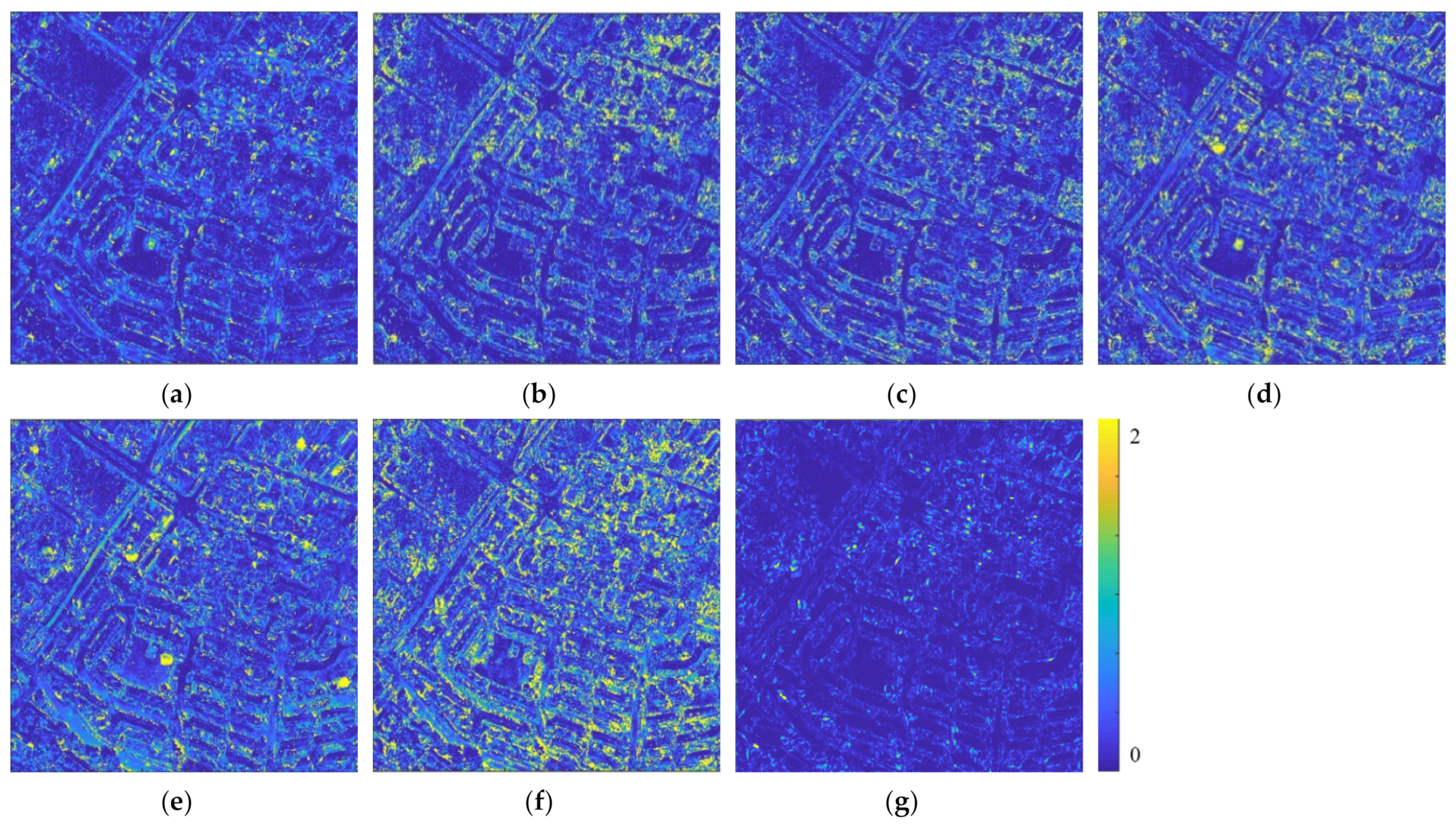
We visualize the fusion results of the proposed method and six comparison methods on Washington DC dataset in Figure 6. Band 16, 82 and 166 are selected as R, G and B bands of the displayed images. Results of GSA, SFIMHS, GLPHS, CNMF are respectively displayed in Figure 6a–d. Results of ICCV15, HySure and the proposed method and the ground truth are presented in Figure 6e–h. To more intuitively compare the results of all methods, we further display their residual difference maps from the ground truth in Figure 7. It can be observed that the result of the proposed method has the least residual information. We also compare the proposed method with other six methods quantitatively in Table 3 which lists the five indexes mentioned above. We mark quantitative evaluation results with the highest scores in bold and those with the second highest scores with underline. The proposed method achieves the highest scores in all five indexes and outperforms the method with the second highest score by a large extent. For co-variance map and RX detection map of results in Washington DC dataset with simulated HR MSI, please view Figures S4 and S9 in Supplementary Materials.
3.3. Experiment with Real Multispectral Images
The experiments presented above assume that HR MSI can be simulated by adding the channels of corresponding HR HSI linearly according to the spectral response function. However, according to reference [6], the actual relationship between HSI and MSI obtained physically is far from linear but non-linear, and it is hard to precisely establish the complex relationship between them. So those methods based on the assumption of simple linear relationship between real HR HSI and HR MSI will not operate well in real applications. However, the proposed method is not based on this assumption and can deal well with complex spectral response function in the real situation.
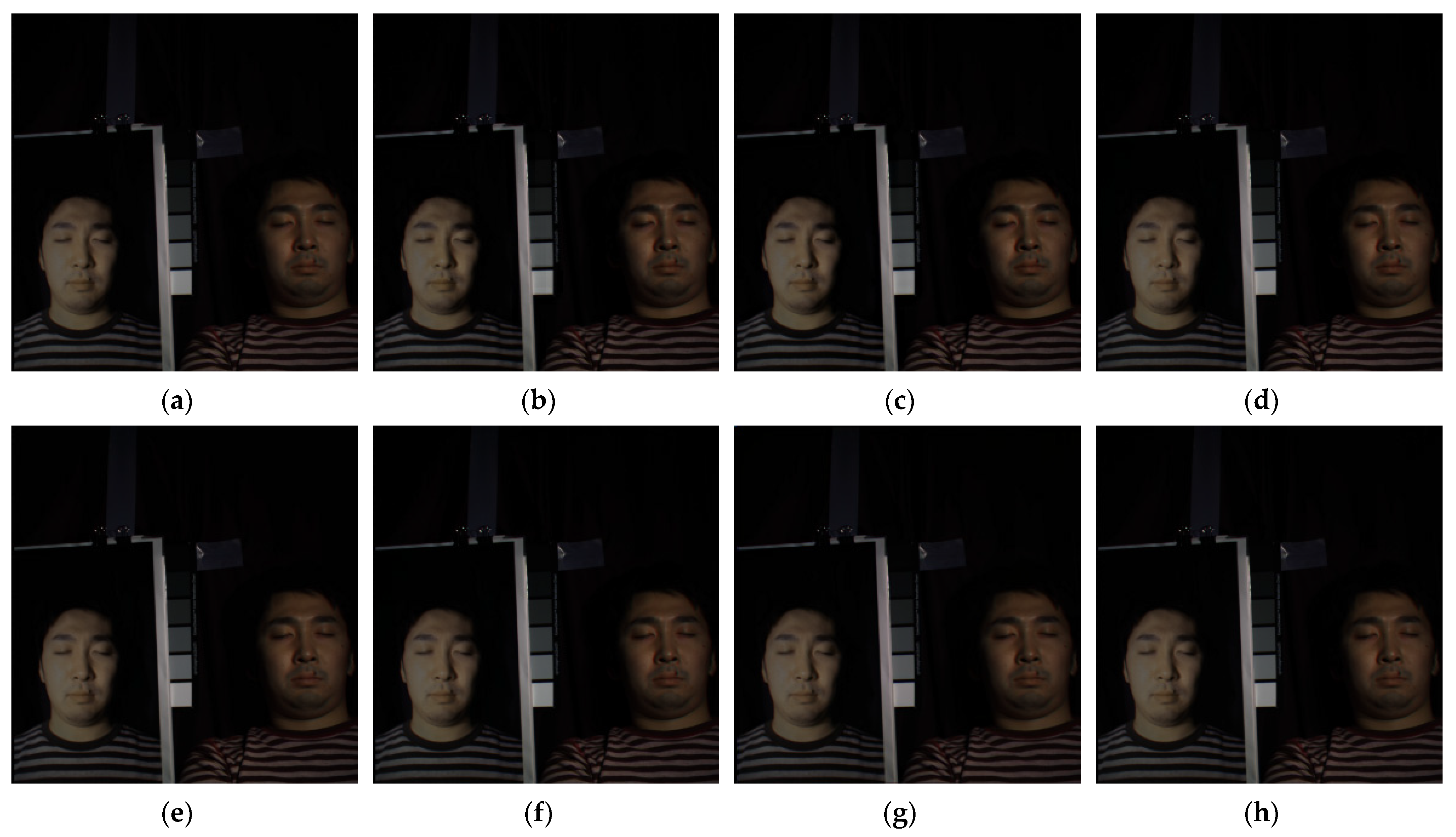
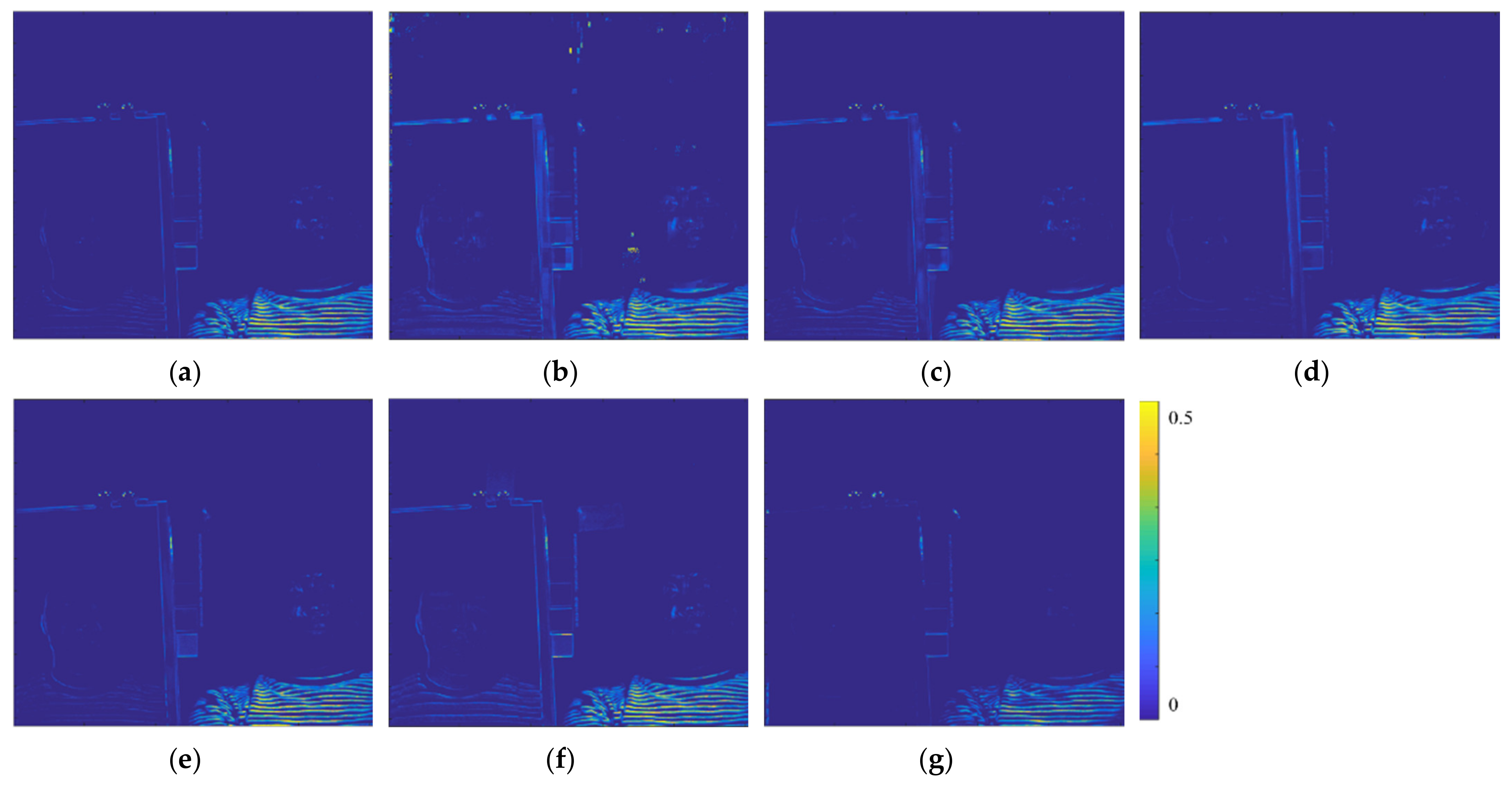
3.3.1. CAVE Dataset
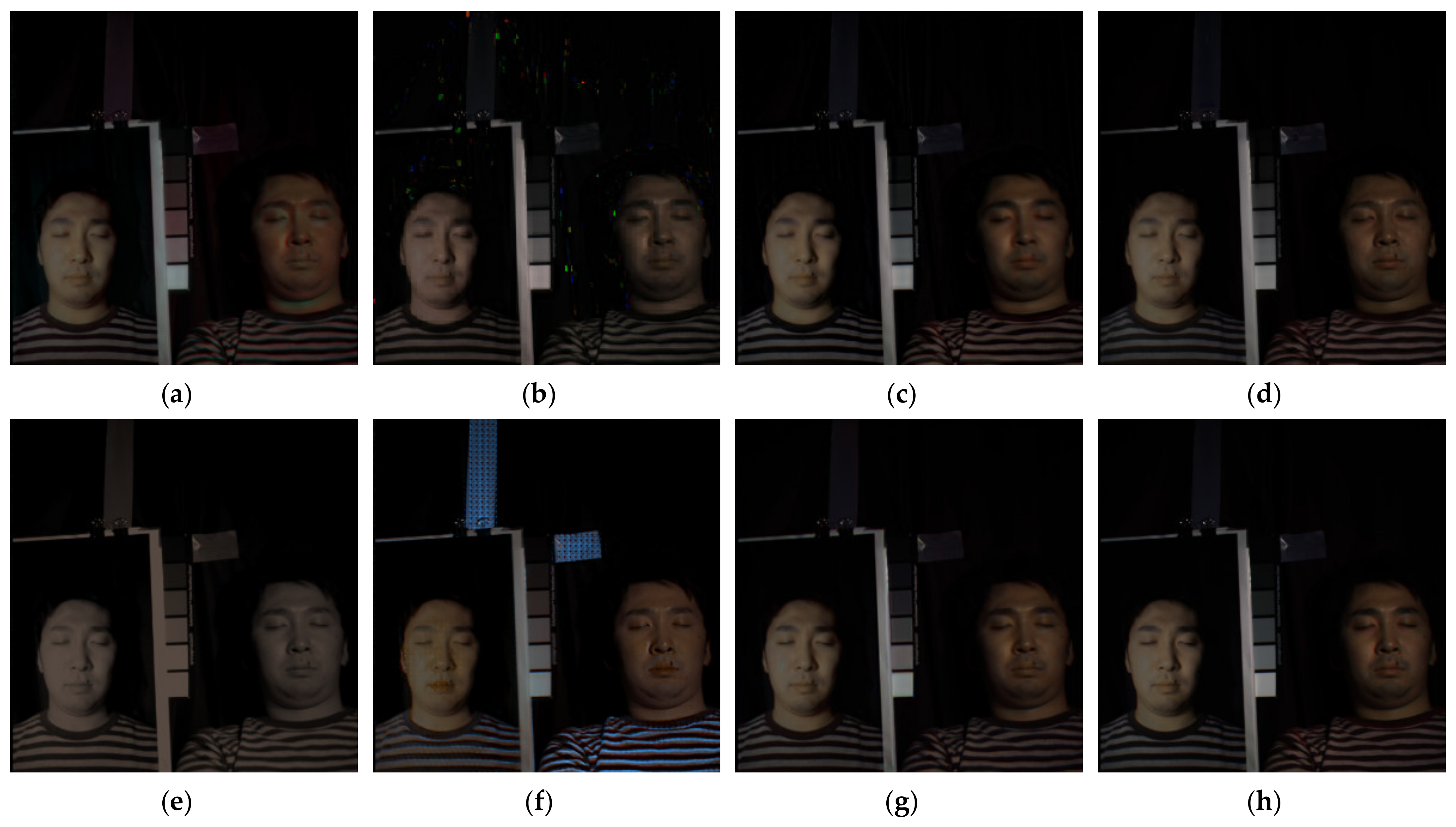
We pick one image among six test images from CAVE and display the fusion results of the proposed method and the comparison method in Figure 8. The 11th, 21st and 31st bands are chosen as the R, G and B bands for visualization. With the real multispectral images in CAVE dataset, all six comparison methods, which are all based on the assumption of simple linear spectral response function, obtain unsatisfying fusion results. We also display the residual information maps of ground truth and results from all methods in Figure 9. In terms of the results of the six comparison methods, there is much more residual information in the experiment with real HR MSI than that in the experiments with simulated HR MSI that are displayed in Figure 3 and Figure 5. It is testified again that the six comparison methods follow the wrong assumption. The proposed method, however, has the least residual information in the fusion results compared with the other six methods in CAVE dataset and has the equivalent residual information in experiments with simulated HR MSI and real HR MSI, which can be observed in Figure 3 and Figure 9. That means the proposed method does not rely on the accuracy of spectral response function and can well perform in real situations. The quantitative evaluation scores of fusion results from all methods are listed in Table 4. We mark the highest scores of indexes in bold and the second highest with underline. It is worth noting that in the experiment of real HR MSI, all six comparison methods cannot obtain the scores as high as those in the experiments with simulated HR MSI, which again indicates that they are not ready for real situations. The proposed method, however, acquires the highest scores in all indexes and outperforms the comparison methods by a large extent. Comparing the quantitative evaluation results of the proposed methods in the experiments of real HR MSI and those in the experiments of simulated HR MSI, the proposed method obtains the same good results in both situations, which again confirms that the proposed method is not constrained by the accuracy of spectral response function and can be practically used. For co-variance map and RX detection map of results in CAVE dataset with real HR MSI, please view Figures S2 and S6 in Supplementary Materials.
3.3.2. Houston 2018 Dataset
We display the fusion results of the proposed method and the comparison method in Figure 10. From Figure 10, we observe that all comparison methods cannot acquire results with sharp spatial details and spectral information at the same time. Compared with these methods, results of the proposed method have accurate spectral and spatial information. We also display the residual information maps of ground truth and results from all methods in Figure 11. The proposed method has the least residual information in the fusion results compared with the other six methods in Houston 2018 dataset. The quantitative evaluation scores of fusion results from all methods are listed in Table 5. The proposed method acquires the highest scores in all indexes and outperforms the comparison methods by a large extent. For co-variance map and RX detection map of results in Houston 2018 dataset with real HR MSI, please view Figures S5 and S10 in Supplementary Materials.
4. Discussion
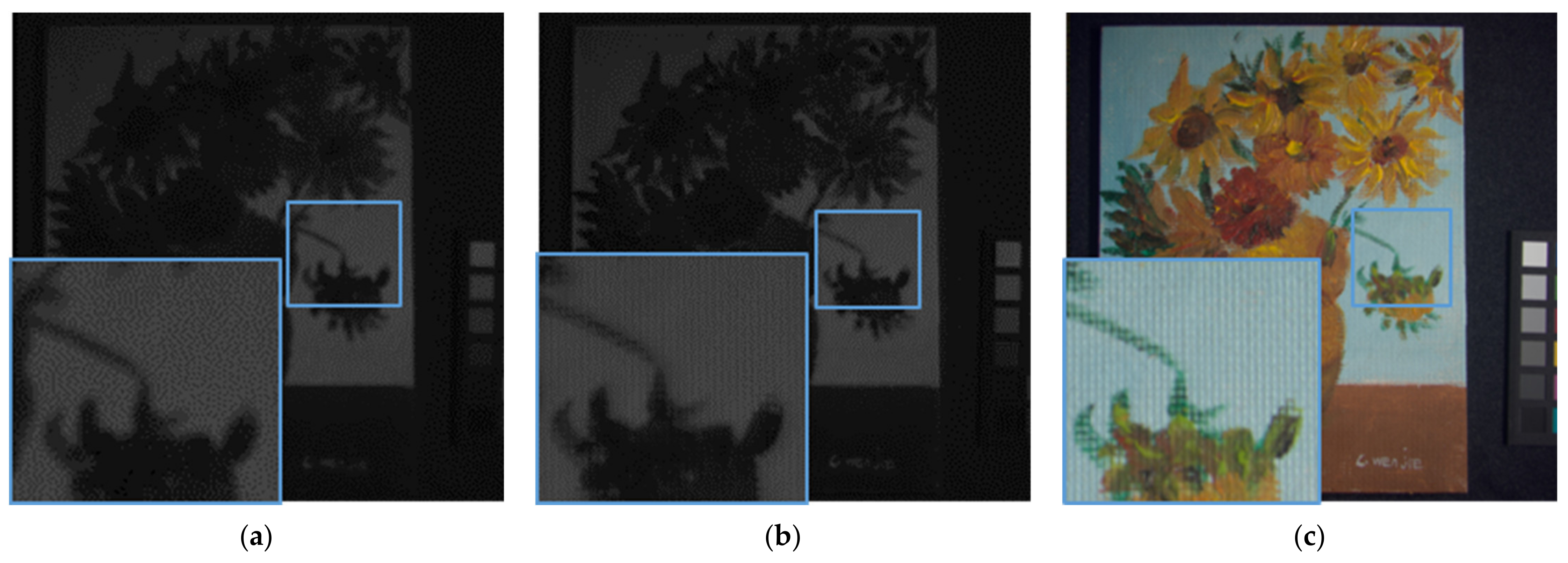
In our experiment results, we find that the proposed method can even obtain enhanced results compared with ground truth images. As is mentioned in reference [17], out-of-focus blur exists at the extremes of the spectral range because different channels are acquired individually in a fixed focal length with the tunable filters. An example is selected from CAVE dataset. The 1st band of hyperspectral image is displayed in Figure 12a. There is no texture information in the 1st band of ground truth image while there is rich texture information in the corresponding RGB image. However, the proposed method can inject the spatial information from the RGB image to this band of the result without largely changing the spectral accuracy, which is shown in Figure 12b.
5. Conclusions
In this paper, we introduce a novel strategy, which makes use of the strong fitting ability of deep neural network to LR HSI and HR MSI fusion task and can operate without training datasets in a self-supervised manner. The spatial information of target is constrained by the fake HR HSI obtained by the spatial diffusion and the spectral accuracy is constrained by LR HSI. A simple deep neural network is used to complete the interpolation process. We conduct several simulation and real-data experiments on some popular hyperspectral datasets to compare the proposed method with other state-of-the-art methods. Quantitative and qualitative results confirm the outperformance and higher accuracy of the proposed methods compared with other fusion methods.
In spite of the great performance of our method, the optimization process costs much time. In our future work, we will train a deep neural network in a self-supervised manner with the proposed strategy and process the images in a feed-forward manner. On the other hand, we will attempt to further improve the accuracy of fusion results by combining other strategies such as recurrence.
Supplementary Materials
The following are available online at https://0-www-mdpi-com.brum.beds.ac.uk/article/10.3390/rs13163226/s1, Figure S1. Curve of spectral difference between selected pixels and ground truth; Figure S2. co-variance matrix of CAVE dataset experiment with real HR MSI; Figure S3. co-variance matrix of CAVE dataset experiment with simulated HR MSI; Figure S4. co-variance matrix of Washington DC dataset experiment with simulated HR MSI; Figure S5. co-variance matrix of Houston 2018 dataset experiment with real HR MSI; Figure S6. co-variance matrix of Pavia dataset experiment with simulation HR MSI; Figure S7. RX map of CAVE dataset experiment with real HR MSI; Figure S8. RX map of CAVE dataset experiment with simulated HR MSI; Figure S9. RX map of Washington DC dataset experiment with real HR MSI; Figure S10. RX map of Houston 2018 dataset experiment with simulated HR MSI; Figure S11. RX map of Pavia dataset experiment with simulated HR MSI.
Author Contributions
Conceptualization, J.G., M.J. and J.L.; Formal analysis, M.J. and J.L.; Funding and acquisition, J.L.; Investigation, J.G.; Methodology, J.G., M.J. and J.L.; Project administration, J.L.; Resources, M.J. and J.L.; Supervision, M.J. and J.L.; Validation, J.G.; Writing—original draft, J.G. and J.L.; Writing—review and editing, M.J. and J.L. All authors have read and agreed to the published version of the manuscript.
Funding
This research was funded by National Key R&D Program of China, grant number 2017YFA0604402, National Natural Science Foundation of China, grant number 62071341.
Data Availability Statement
Publicly available datasets were analyzed in this study. This data can be found here: CAVE dataset is from https://www.cs.columbia.edu/CAVE/databases/multispectral/ (accessed on 12 August 2021); Houston 2018 dataset is from https://hyperspectral.ee.uh.edu/?page_id=1075 (accessed on 12 August 2021); Pavia University dataset is from http://www.ehu.eus/ccwintco/index.php/Hyperspectral_Remote_Sensing_Scenes (accessed on 12 August 2021).
Conflicts of Interest
The authors declare no conflict of interest.
References
- Zhang, F.; Du, B.; Zhang, L. Scene classification via a gradient boosting random convolutional network framework. IEEE Trans. Geosci. Remote. Sens. 2015, 54, 1793–1802. [Google Scholar] [CrossRef]
- Uzkent, B.; Rangnekar, A.; Hoffman, M. Aerial vehicle tracking by adaptive fusion of hyperspectral likelihood maps. In Proceedings of the IEEE Conference on Computer Vision and Pattern Recognition Workshops, Honolulu, HI, USA, 21–26 July 2017; pp. 39–48. [Google Scholar]
- Plaza, A.; Du, Q.; Bioucas-Dias, J.M.; Jia, X.; Kruse, F.A. Foreword to the special issue on spectral unmixing of remotely sensed data. IEEE Trans. Geosci. Remote. Sens. 2011, 49, 4103–4110. [Google Scholar] [CrossRef] [Green Version]
- Du, L.; Tian, Q.; Yu, T.; Meng, Q.; Jancso, T.; Udvardy, P.; Huang, Y. A comprehensive drought monitoring method integrating MODIS and TRMM data. Int. J. Appl. Earth Obs. Geoinf. 2013, 23, 245–253. [Google Scholar] [CrossRef]
- Rodríguez-Veiga, P.; Quegan, S.; Carreiras, J.; Persson, H.J.; Fransson, J.E.; Hoscilo, A.; Ziółkowski, D.; Stereńczak, K.; Lohberger, S.; Stängel, M. Forest biomass retrieval approaches from earth observation in different biomes. Int. J. Appl. Earth Obs. Geoinf. 2019, 77, 53–68. [Google Scholar] [CrossRef]
- Yokoya, N.; Grohnfeldt, C.; Chanussot, J. Hyperspectral and multispectral data fusion: A comparative review of the recent literature. IEEE Geosci. Remote Sens. Mag. 2017, 5, 29–56. [Google Scholar] [CrossRef]
- Kwarteng, P.; Chavez, A. Extracting spectral contrast in Landsat Thematic Mapper image data using selective principal component analysis. Photogramm. Eng. Remote. Sens. 1989, 55, 339–348. [Google Scholar]
- Carper, W.; Lillesand, T.; Kiefer, R. The use of intensity-hue-saturation transformations for merging SPOT panchromatic and multispectral image data. Photogramm. Eng. Remote. Sens. 1990, 56, 459–467. [Google Scholar]
- Laben, C.A.; Brower, B.V. Process for Enhancing the Spatial Resolution of Multispectral Imagery Using Pan-Sharpening. U.S. Patent No. 6,011,875, 1 April 2000. [Google Scholar]
- Aiazzi, B.; Baronti, S.; Selva, M. Improving component substitution pansharpening through multivariate regression of MS + Pan data. IEEE Trans. Geosci. Remote. Sens. 2007, 45, 3230–3239. [Google Scholar] [CrossRef]
- Chavez, P.; Sides, S.C.; Anderson, J.A. Comparison of three different methods to merge multiresolution and multispectral data- Landsat TM and SPOT panchromatic. Photogramm. Eng. Remote. Sens. 1991, 57, 295–303. [Google Scholar]
- Liu, J. Smoothing filter-based intensity modulation: A spectral preserve image fusion technique for improving spatial details. Int. J. Remote. Sens. 2000, 21, 3461–3472. [Google Scholar] [CrossRef]
- Aiazzi, B.; Alparone, L.; Baronti, S.; Garzelli, A.; Selva, M. MTF-tailored multiscale fusion of high-resolution MS and Pan imagery. Photogramm. Eng. Remote. Sens. 2006, 72, 591–596. [Google Scholar] [CrossRef]
- Shahdoosti, H.R.; Javaheri, N. Pansharpening of clustered MS and Pan images considering mixed pixels. IEEE Geosci. Remote Sens. Lett. 2017, 14, 826–830. [Google Scholar] [CrossRef]
- Yasuma, F.; Mitsunaga, T.; Iso, D.; Nayar, S.K. Generalized assorted pixel camera: Postcapture control of resolution, dynamic range, and spectrum. IEEE Trans. Image Process. 2010, 19, 2241–2253. [Google Scholar] [CrossRef] [Green Version]
- Iordache, M.-D.; Bioucas-Dias, J.M.; Plaza, A. Sparse unmixing of hyperspectral data. IEEE Trans. Geosci. Remote. Sens. 2011, 49, 2014–2039. [Google Scholar] [CrossRef] [Green Version]
- Yokoya, N.; Yairi, T.; Iwasaki, A. Coupled nonnegative matrix factorization unmixing for hyperspectral and multispectral data fusion. IEEE Trans. Geosci. Remote. Sens. 2011, 50, 528–537. [Google Scholar] [CrossRef]
- Akhtar, N.; Shafait, F.; Mian, A. Sparse spatio-spectral representation for hyperspectral image super-resolution. In Proceedings of the European Conference on Computer Vision, Glasgow, UK, 23–28 August 2020; pp. 63–78. [Google Scholar]
- Akhtar, N.; Shafait, F.; Mian, A. Bayesian sparse representation for hyperspectral image super resolution. In Proceedings of the IEEE Conference on Computer Vision and Pattern Recognition, Boston, MA, USA, 7–12 June 2015; pp. 3631–3640. [Google Scholar]
- Lanaras, C.; Baltsavias, E.; Schindler, K. Hyperspectral super-resolution by coupled spectral unmixing. In Proceedings of the IEEE International Conference on Computer Vision, Santiago, Chile, 7–13 December 2015; pp. 3586–3594. [Google Scholar]
- Zhang, L.; Shen, H.; Gong, W.; Zhang, H. Adjustable model-based fusion method for multispectral and panchromatic images. IEEE Trans. Syst. Man Cybern. Part. B (Cybern.) 2012, 42, 1693–1704. [Google Scholar] [CrossRef] [PubMed]
- Chatterjee, A.; Yuen, P.W. Endmember learning with k-means through scd model in hyperspectral scene reconstructions. J. Imaging 2019, 5, 85. [Google Scholar] [CrossRef] [Green Version]
- Zhang, L.; Nie, J.; Wei, W.; Li, Y.; Zhang, Y. Deep Blind Hyperspectral Image Super-Resolution. IEEE Trans. Neural Netw. Learn. Syst. 2020, 32, 2388–2400. [Google Scholar] [CrossRef] [PubMed]
- Yang, S.; Zhang, K.; Wang, M. Learning low-rank decomposition for pan-sharpening with spatial-spectral offsets. IEEE Trans. Neural Netw. Learn. Syst. 2017, 29, 3647–3657. [Google Scholar]
- Zhou, Y.; Feng, L.; Hou, C.; Kung, S.-Y. Hyperspectral and multispectral image fusion based on local low rank and coupled spectral unmixing. IEEE Trans. Geosci. Remote. Sens. 2017, 55, 5997–6009. [Google Scholar] [CrossRef]
- Liu, X.; Shen, H.; Yuan, Q.; Lu, X.; Zhou, C. A universal destriping framework combining 1-D and 2-D variational optimization methods. IEEE Trans. Geosci. Remote. Sens. 2017, 56, 808–822. [Google Scholar] [CrossRef]
- Shen, H. Integrated fusion method for multiple temporal-spatial-spectral images. In Proceedings of the 22nd ISPRS Congress, Melbourne, Australia, 5 August–1 September 2012; Volume B7, pp. 407–410. [Google Scholar] [CrossRef] [Green Version]
- Han, X.-H.; Zheng, Y.; Chen, Y.-W. Multi-level and multi-scale spatial and spectral fusion CNN for hyperspectral image super-resolution. In Proceedings of the IEEE/CVF International Conference on Computer Vision Workshops, Seoul, Korea, 27–28 October 2019. [Google Scholar]
- Palsson, F.; Sveinsson, J.R.; Ulfarsson, M.O. Multispectral and hyperspectral image fusion using a 3-D-convolutional neural network. IEEE Geosci. Remote Sens. Lett. 2017, 14, 639–643. [Google Scholar] [CrossRef] [Green Version]
- Mei, S.; Yuan, X.; Ji, J.; Zhang, Y.; Wan, S.; Du, Q. Hyperspectral image spatial super-resolution via 3D full convolutional neural network. Remote. Sens. 2017, 9, 1139. [Google Scholar] [CrossRef] [Green Version]
- Xie, Q.; Zhou, M.; Zhao, Q.; Meng, D.; Zuo, W.; Xu, Z. Multispectral and hyperspectral image fusion by MS/HS fusion net. In Proceedings of the IEEE/CVF Conference on Computer Vision and Pattern Recognition, Long Beach, CA, USA, 15–20 June 2019; pp. 1585–1594. [Google Scholar]
- Liu, S.; Miao, S.; Su, J.; Li, B.; Hu, W.; Zhang, Y.-D. UMAG-Net: A New Unsupervised Multi-attention-guided Network for Hyperspectral and Multispectral Image Fusion. IEEE J. Sel. Top. Appl. Earth Obs. Remote. Sens. 2021, 14, 7373–7385. [Google Scholar] [CrossRef]
- Lu, X.; Zhang, J.; Yang, D.; Xu, L.; De Jia, F. Cascaded Convolutional Neural Network-Based Hyperspectral Image Resolution Enhancement via an Auxiliary Panchromatic Image. IEEE Trans. Image Process. 2021, 30, 6815–6828. [Google Scholar] [CrossRef]
- Gatys, L.A.; Ecker, A.S.; Bethge, M. Image style transfer using convolutional neural networks. In Proceedings of the IEEE Conference on Computer Vision and Pattern Recognition, Las Vegas, NV, USA, 27–30 June 2016; pp. 2414–2423. [Google Scholar]
- Ulyanov, D.; Vedaldi, A.; Lempitsky, V. Deep image prior. In Proceedings of the IEEE Conference on Computer Vision and Pattern Recognition, Salt Lake City, UT, USA, 18–23 June 2018; pp. 9446–9454. [Google Scholar]
- Shaham, T.R.; Dekel, T.; Michaeli, T. Singan: Learning a generative model from a single natural image. In Proceedings of the IEEE/CVF International Conference on Computer Vision, Seoul, Korea, 27 October–2 November 2019; pp. 4570–4580. [Google Scholar]
- Shocher, A.; Bagon, S.; Isola, P.; Irani, M. Ingan: Capturing and retargeting the "DNA" of a natural image. In Proceedings of the IEEE/CVF International Conference on Computer Vision, Seoul, Korea, 27 October–2 November 2019; pp. 4492–4501. [Google Scholar]
- Simonyan, K.; Zisserman, A. Very deep convolutional networks for large-scale image recognition. arXiv Prepr. 2014, arXiv:1409.1556. [Google Scholar]
- Gatys, L.; Ecker, A.S.; Bethge, M. Texture synthesis using convolutional neural networks. Adv. Neural Inf. Process. Syst. 2015, 28, 262–270. [Google Scholar]
- Selva, M.; Aiazzi, B.; Butera, F.; Chiarantini, L.; Baronti, S. Hyper-sharpening: A first approach on SIM-GA data. IEEE J. Sel. Top. Appl. Earth Obs. Remote. Sens. 2015, 8, 3008–3024. [Google Scholar] [CrossRef]
- Simoes, M.; Bioucas-Dias, J.; Almeida, L.B.; Chanussot, J. A convex formulation for hyperspectral image superresolution via subspace-based regularization. IEEE Trans. Geosci. Remote. Sens. 2014, 53, 3373–3388. [Google Scholar] [CrossRef] [Green Version]
Figure 1.
Framework of our method.

Figure 2.
Results of CAVE dataset with simulated multispectral images. (a) results of GSA; (b) results of SFIMHS; (c) results of GLPHS; (d) results of CNMF; (e) results of ICCV15; (f) results of HySure; (g) ours results; (h) Ground truth.
Figure 2.
Results of CAVE dataset with simulated multispectral images. (a) results of GSA; (b) results of SFIMHS; (c) results of GLPHS; (d) results of CNMF; (e) results of ICCV15; (f) results of HySure; (g) ours results; (h) Ground truth.

Figure 3.
Residual information of CAVE dataset with simulated multispectral images. (a) results of GSA; (b) results of SFIMHS; (c) results of GLPHS; (d) results of CNMF; (e) results of ICCV15; (f) results of HySure; (g) ours results.
Figure 3.
Residual information of CAVE dataset with simulated multispectral images. (a) results of GSA; (b) results of SFIMHS; (c) results of GLPHS; (d) results of CNMF; (e) results of ICCV15; (f) results of HySure; (g) ours results.

Figure 4.
Results of Pavia University dataset with simulated multispectral images. (a) results of GSA; (b) results of SFIMHS; (c) results of GLPHS; (d) results of CNMF; (e) results of ICCV15; (f) results of HySure; (g) ours results; (h) Ground truth.
Figure 4.
Results of Pavia University dataset with simulated multispectral images. (a) results of GSA; (b) results of SFIMHS; (c) results of GLPHS; (d) results of CNMF; (e) results of ICCV15; (f) results of HySure; (g) ours results; (h) Ground truth.
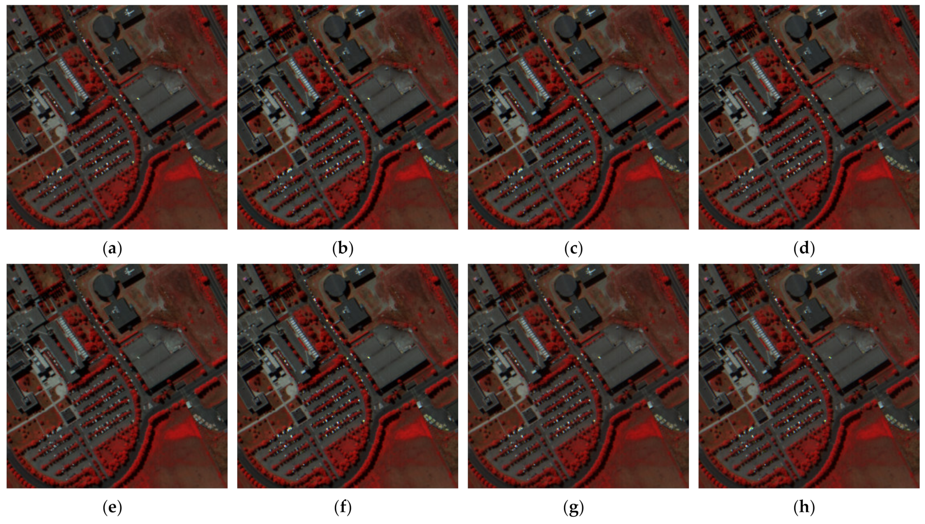
Figure 5.
Residual information of Pavia University dataset with simulated multispectral images. (a) results of GSA; (b) results of SFIMHS; (c) results of GLPHS; (d) results of CNMF; (e) results of ICCV15; (f) results of HySure; (g) ours results.
Figure 5.
Residual information of Pavia University dataset with simulated multispectral images. (a) results of GSA; (b) results of SFIMHS; (c) results of GLPHS; (d) results of CNMF; (e) results of ICCV15; (f) results of HySure; (g) ours results.

Figure 6.
Results of Washington DC dataset with simulated multispectral images. (a) results of GSA; (b) results of SFIMHS; (c) results of GLPHS; (d) results of CNMF; (e) results of ICCV15; (f) results of HySure; (g) ours results; (h) Ground truth.
Figure 6.
Results of Washington DC dataset with simulated multispectral images. (a) results of GSA; (b) results of SFIMHS; (c) results of GLPHS; (d) results of CNMF; (e) results of ICCV15; (f) results of HySure; (g) ours results; (h) Ground truth.

Figure 7.
Residual information of Washington DC dataset with simulated multispectral images. (a) results of GSA; (b) results of SFIMHS; (c) results of GLPHS; (d) results of CNMF; (e) results of ICCV15; (f) results of HySure; (g) ours results.
Figure 7.
Residual information of Washington DC dataset with simulated multispectral images. (a) results of GSA; (b) results of SFIMHS; (c) results of GLPHS; (d) results of CNMF; (e) results of ICCV15; (f) results of HySure; (g) ours results.

Figure 8.
Results of CAVE dataset with real multispectral images. (a) results of GSA; (b) results of SFIMHS; (c) results of GLPHS; (d) results of CNMF; (e) results of ICCV15; (f) results of HySure; (g) ours results; (h) Ground truth.
Figure 8.
Results of CAVE dataset with real multispectral images. (a) results of GSA; (b) results of SFIMHS; (c) results of GLPHS; (d) results of CNMF; (e) results of ICCV15; (f) results of HySure; (g) ours results; (h) Ground truth.

Figure 9.
Residual information of CAVE dataset with real multispectral images. (a) results of GSA; (b) results of SFIMHS; (c) results of GLPHS; (d) results of CNMF; (e) results of ICCV15; (f) results of HySure; (g) ours results.
Figure 9.
Residual information of CAVE dataset with real multispectral images. (a) results of GSA; (b) results of SFIMHS; (c) results of GLPHS; (d) results of CNMF; (e) results of ICCV15; (f) results of HySure; (g) ours results.

Figure 10.
Results of Houston 2018 dataset with real multispectral images. (a) results of GSA; (b) results of SFIMHS; (c) results of GLPHS; (d) results of CNMF; (e) results of ICCV15; (f) results of HySure; (g) ours results; (h) Ground truth.
Figure 10.
Results of Houston 2018 dataset with real multispectral images. (a) results of GSA; (b) results of SFIMHS; (c) results of GLPHS; (d) results of CNMF; (e) results of ICCV15; (f) results of HySure; (g) ours results; (h) Ground truth.

Figure 11.
Residual information of Houston 2018 dataset with real multispectral images. (a) results of GSA; (b) results of SFIMHS; (c) results of GLPHS; (d) results of CNMF; (e) results of ICCV15; (f) results of HySure; (g) ours results.
Figure 11.
Residual information of Houston 2018 dataset with real multispectral images. (a) results of GSA; (b) results of SFIMHS; (c) results of GLPHS; (d) results of CNMF; (e) results of ICCV15; (f) results of HySure; (g) ours results.

Figure 12.
Enhancement from ground truth. (a) 1st band of ground truth; (b) 1st band of ours; (c) original RGB image.
Figure 12.
Enhancement from ground truth. (a) 1st band of ground truth; (b) 1st band of ours; (c) original RGB image.


Table 1.
Quantitative evaluation results of CAVE dataset with simulated multispectral images.
| PSNR | SSIM | SAM | CC | |
|---|---|---|---|---|
| GSA | 38.4838 | 0.9742 | 4.5940 | 0.9745 |
| SFIMHS | 33.8042 | 0.9396 | 8.7843 | 0.9641 |
| CNMF | 34.8185 | 0.9506 | 7.6047 | 0.9109 |
| ICCV15 | 36.5875 | 0.9652 | 6.0231 | 0.9766 |
| GLPHS | 37.4164 | 0.9606 | 5.5818 | 0.9769 |
| HySure | 37.3821 | 0.9585 | 6.7477 | 0.9641 |
| Ours | 40.1032 | 0.9864 | 4.2902 | 0.9832 |
Scores marked in bold mean the best and those marked with underline mean the second best.
Table 2.
Quantitative evaluation results of Pavia University dataset with simulated multispectral images.
Table 2.
Quantitative evaluation results of Pavia University dataset with simulated multispectral images.
| PSNR | SSIM | SAM | CC | |
|---|---|---|---|---|
| GSA | 38.0679 | 0.9721 | 3.6394 | 0.9337 |
| SFIMHS | 35.8753 | 0.9651 | 4.0605 | 0.9343 |
| CNMF | 37.6781 | 0.9720 | 3.6576 | 0.9335 |
| ICCV15 | 38.3872 | 0.9737 | 3.3430 | 0.9220 |
| GLPHS | 37.6992 | 0.9742 | 3.3215 | 0.9178 |
| HySure | 35.7145 | 0.9676 | 3.6405 | 0.9215 |
| Ours | 38.7403 | 0.9751 | 3.2625 | 0.9345 |
Scores marked in bold mean the best and those marked with underline mean the second best.
Table 3.
Quantitative evaluation results of Washington DC dataset with simulated multispectral images.
Table 3.
Quantitative evaluation results of Washington DC dataset with simulated multispectral images.
| PSNR | SSIM | SAM | CC | |
|---|---|---|---|---|
| GSA | 38.6088 | 0.9839 | 1.9482 | 0.9932 |
| SFIMHS | 36.4287 | 0.9817 | 2.2033 | 0.9924 |
| CNMF | 38.3836 | 0.9857 | 1.8832 | 0.9929 |
| ICCV15 | 36.9171 | 0.9696 | 2.2603 | 0.9767 |
| GLPHS | 37.5585 | 0.9763 | 2.1159 | 0.9750 |
| HySure | 37.5309 | 0.9805 | 1.9879 | 0.9901 |
| Ours | 39.1805 | 0.9873 | 1.6875 | 0.9937 |
Scores marked in bold mean the best and those marked with underline mean the second best.
Table 4.
Quantitative evaluation results of CAVE dataset with real multispectral images.
| PSNR | SSIM | SAM | CC | |
|---|---|---|---|---|
| GSA | 30.3058 | 0.8591 | 13.8931 | 0.9727 |
| SFIMHS | 25.2277 | 0.8126 | 22.3912 | 0.9244 |
| CNMF | 30.6975 | 0.8908 | 10.7764 | 0.9496 |
| ICCV15 | 27.1515 | 0.8811 | 12.9924 | 0.9412 |
| GLPHS | 35.0865 | 0.9262 | 8.4063 | 0.9829 |
| HySure | 27.7137 | 0.8312 | 14.7039 | 0.9482 |
| Ours | 36.0586 | 0.9601 | 6.6032 | 0.9863 |
Scores marked in bold mean the best and those marked with underline mean the second best.
Table 5.
Quantitative evaluation results of Houston 2018 dataset with real multispectral images.
| PSNR | SSIM | SAM | CC | |
|---|---|---|---|---|
| GSA | 24.2119 | 0.5682 | 9.4216 | 0.9995 |
| SFIMHS | 22.6962 | 0.5431 | 11.0776 | 0.9996 |
| CNMF | 24.4170 | 0.5633 | 8.0521 | 0.9996 |
| ICCV15 | 18.8145 | 0.3710 | 18.2986 | 0.9961 |
| GLPHS | 24.6457 | 0.5935 | 8.5538 | 0.9990 |
| HySure | 23.6509 | 0.5699 | 8.0248 | 0.9994 |
| Ours | 27.1543 | 0.6772 | 7.4625 | 0.9997 |
Scores marked in bold mean the best and those marked with underline mean the second best.
Publisher’s Note: MDPI stays neutral with regard to jurisdictional claims in published maps and institutional affiliations. |
© 2021 by the authors. Licensee MDPI, Basel, Switzerland. This article is an open access article distributed under the terms and conditions of the Creative Commons Attribution (CC BY) license (https://creativecommons.org/licenses/by/4.0/).
Share and Cite
MDPI and ACS Style
Gao, J.; Li, J.; Jiang, M. Hyperspectral and Multispectral Image Fusion by Deep Neural Network in a Self-Supervised Manner. Remote Sens. 2021, 13, 3226. https://0-doi-org.brum.beds.ac.uk/10.3390/rs13163226
AMA Style
Gao J, Li J, Jiang M. Hyperspectral and Multispectral Image Fusion by Deep Neural Network in a Self-Supervised Manner. Remote Sensing. 2021; 13(16):3226. https://0-doi-org.brum.beds.ac.uk/10.3390/rs13163226
Chicago/Turabian StyleGao, Jianhao, Jie Li, and Menghui Jiang. 2021. "Hyperspectral and Multispectral Image Fusion by Deep Neural Network in a Self-Supervised Manner" Remote Sensing 13, no. 16: 3226. https://0-doi-org.brum.beds.ac.uk/10.3390/rs13163226
Note that from the first issue of 2016, this journal uses article numbers instead of page numbers. See further details here.