1. Introduction
Invasive species are a global problem with many negative impacts. An estimated USD 120 billion in damage is done annually by these species in the United States alone [
1].
Phragmites australis (Cav.) Trin. Ex Steud. ssp.
australis (hereafter
Phragmites) is an invasive plant that has impaired wetlands, shorelines, and roadsides in the Great Lakes region and across much of the United States. It is a perennial grass that grows in a range of habitats from aquatic to terrestrial.
Phragmites was originally introduced to the United States in the form of contaminated ballast material in the 18th or 19th centuries [
2]. The regulatory status of
Phragmites varies from state to state. In the state of Michigan,
Phragmites is listed as a restricted plant [
3], while in the state of Minnesota, its status was recently changed from a restricted noxious weed to a prohibited control species [
4]. In Minnesota, restricted noxious weeds are plants whose importation, sale, and transportation are illegal. Prohibited control species share the same legalities with restricted noxious weeds for preventing spread; however, these species are legally required to be controlled by removing established populations.
Phragmites grows rapidly with the potential to reach up to 5 m tall. After becoming established,
Phragmites quickly forms dense monotypic stands by using aerial seed dispersal and extensive networks of rhizomes.
Phragmites can quickly become the dominant species in invaded areas due to fast growth rates [
5], salinity tolerance [
6], and by taking advantage of anthropogenic impacts to wetlands [
7]. Examples of anthropogenic impacts include: removal of vegetation, soil removal or deposition, fragmentation, and pollutant runoff. Once established, this plant has the ability to alter hydrology [
8], change nutrient cycles [
9,
10,
11], and ultimately lead to a loss of biodiversity [
12,
13]. Minnesota also has populations of a native
Phragmites genotype (
Phragmites australis Trin. Ex. Steud. ssp.
americanus Saltonst., P.M. Peterson and Soreng). In comparison, this native genotype does not exhibit the same growth and aggressiveness as the invasive
Phragmites genotype. Native
Phragmites has a smaller stature and generally does not form dense monotypic stands. Invasive
Phragmites is spreading quickly in Minnesota and will likely see an expansion of its distribution [
14].
Successful management of invasive species, such as
Phragmites, depends heavily on knowing the location and extent of infestations. Physical mapping of invasive species, in the form of in situ monitoring, may be costly and requires large amounts of time and specialized equipment to access the locations of infestations. This, coupled with the inter- and-intra annual changes in distributions, leads to challenges for land managers attempting to control these pests. Current knowledge of
Phragmites locations in Minnesota has been dependent on in situ monitoring. Individuals have reported
Phragmites throughout the state through the Early Detection and Distribution Mapping System (EDDMapS) [
15]. Although a remarkable resource, large-scale in situ mapping efforts cannot be completed quickly enough to track the changing distribution of
Phragmites. Moreover, these survey methods may be hindered by a lack of access to private lands, physical inaccessibility of remote locations, and individuals unwilling to report locations.
Remote sensing has the potential to identify
Phragmites over large areas without the requirement of extensive fieldwork. Satellites are collecting swaths of imagery daily, which can be acquired at minimal cost due to increased platform accessibility (Landsat or Sentinel) or through affiliations (university, federal, etc.). Occupied aircraft and unoccupied aircraft systems (UAS) are other often-used remote sensing technologies for conservation purposes [
16,
17,
18]. Although occupied aircraft and UAS require upfront costs, such as equipment purchases or contractual services, and often lack the spectral resolution found in satellite-based platforms, they allow for spatial resolutions of less than 10 cm and flexible data acquisition. Each of these data have trade-offs between spatial, spectral, and temporal resolutions [
19,
20,
21]. Research is needed to assess the different data and classification methods for remote sensing to be a viable tool for
Phragmites detection.
Recent research has tested the use of remote sensing data for species identification. Hyperspectral sensors have been used to identify different vegetation types [
22,
23,
24], including
Phragmites [
25]. Pengra et al. (2007) [
25] used the EO-1 Hyperion hyperspectral sensor to identify
Phragmites. It was noted that the moderate spatial resolution of the Hyperion sensor (30 m) hindered the identification of linear patches of
Phragmites due to mixing of vegetation types within a pixel. Bourgeau-Chavez et al. (2013) [
26] used a similar spatial resolution (20–30 m PALSAR and Landsat). They utilized backscatter intensities from multiple acquisitions of synthetic aperture radar (SAR) imagery to identify
Phragmites with high producer’s accuracies. SAR has been used extensively for vegetation identification and monitoring [
27,
28,
29,
30,
31,
32] because the backscattered energy is indicative of the geometric and dielectric properties of surface features [
33]. Spaceborne sensors with higher spatial resolutions have also been studied for wetland and species mapping [
34,
35,
36,
37,
38,
39,
40]. Laba et al. (2008) [
39] reported consistently high accuracies for identifying
Phragmites using QuickBird imagery and a maximum-likelihood classifier. They attributed the monotypic nature of
Phragmites and the resulting consistent spectral values for accuracies of above 70%. Another study used an object-based classification approach with WorldView-2 imagery to achieve classification accuracies of
Phragmites above 90% [
40]. The high accuracies seen when using high-resolution satellite imagery for mapping invasive species has been validated by others [
41,
42,
43].
To date, there are multiple satellite platforms that offer spatial resolutions higher than two meters. However, some researchers have expressed the need for even higher spatial resolutions for tracking plant invasions [
44,
45]. In that regard, UAS have gained popularity as a tool for invasive species detection due to high spatial and temporal resolution, relatively low cost, and their ability to survey locations quickly. Many have explored the use of UAS for identifying and monitoring invasive
Phragmites [
46,
47,
48]. Samiappan et al. (2017) [
46] indicated that a maximum likelihood classifier with the use of textural algorithms could identify
Phragmites from UAS imagery with average accuracies above 85%. The use of texture to identify
Phragmites from UAS imagery has been studied by others. Abeysinghe et al. (2019) [
47] used image texture, normalized difference vegetation index (NDVI), and a canopy height model (CHM) to identify
Phragmites within an estuary in Lake Erie. They noted the importance of using a CHM to identify Phragmites.
Phragmites is taller than most wetland vegetation, and others have demonstrated the importance of using height for vegetation classification [
49]. After patches had been identified, Tóth (2018) [
48] demonstrated the potential for tracking and monitoring changes in distribution through the use of NDVI.
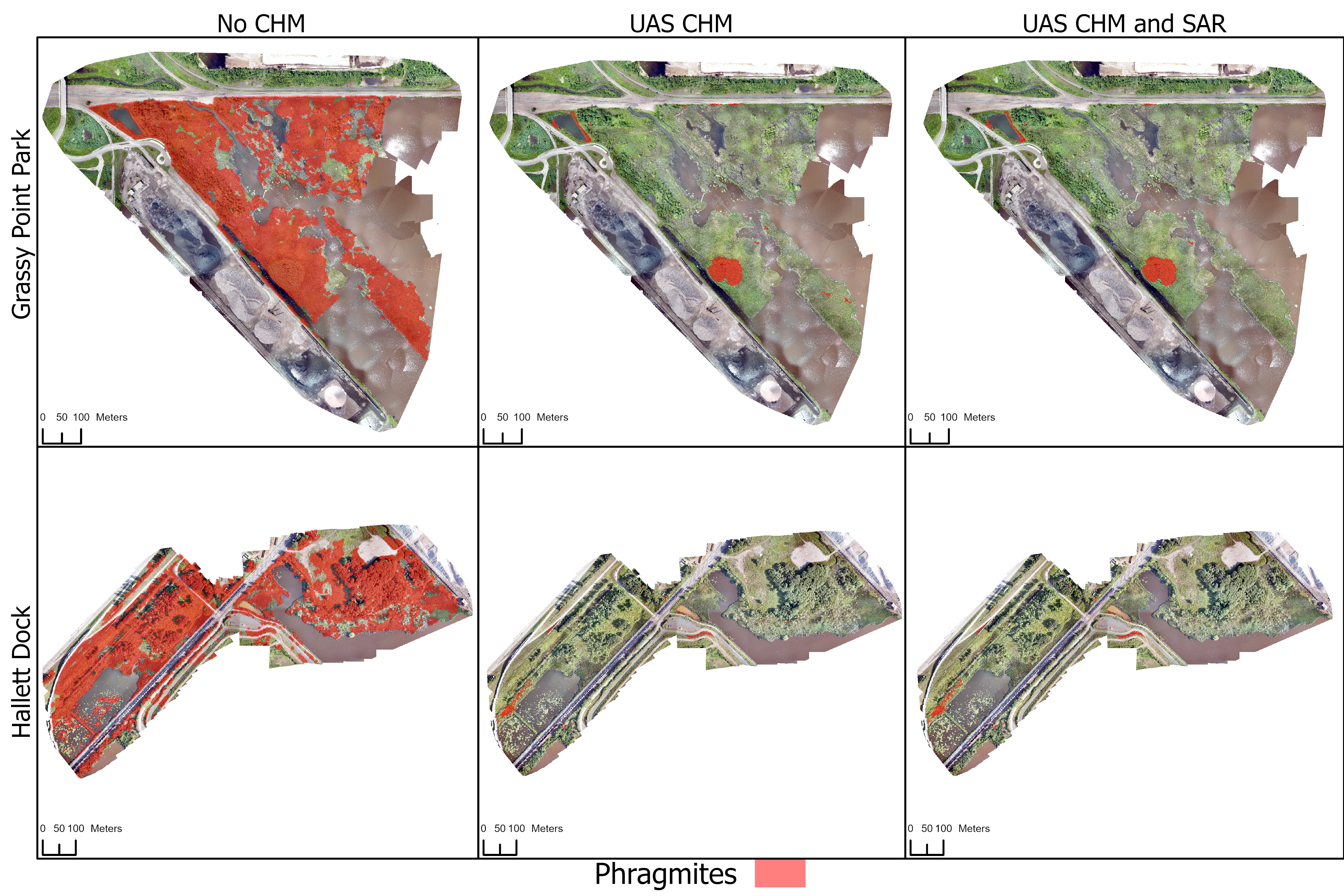
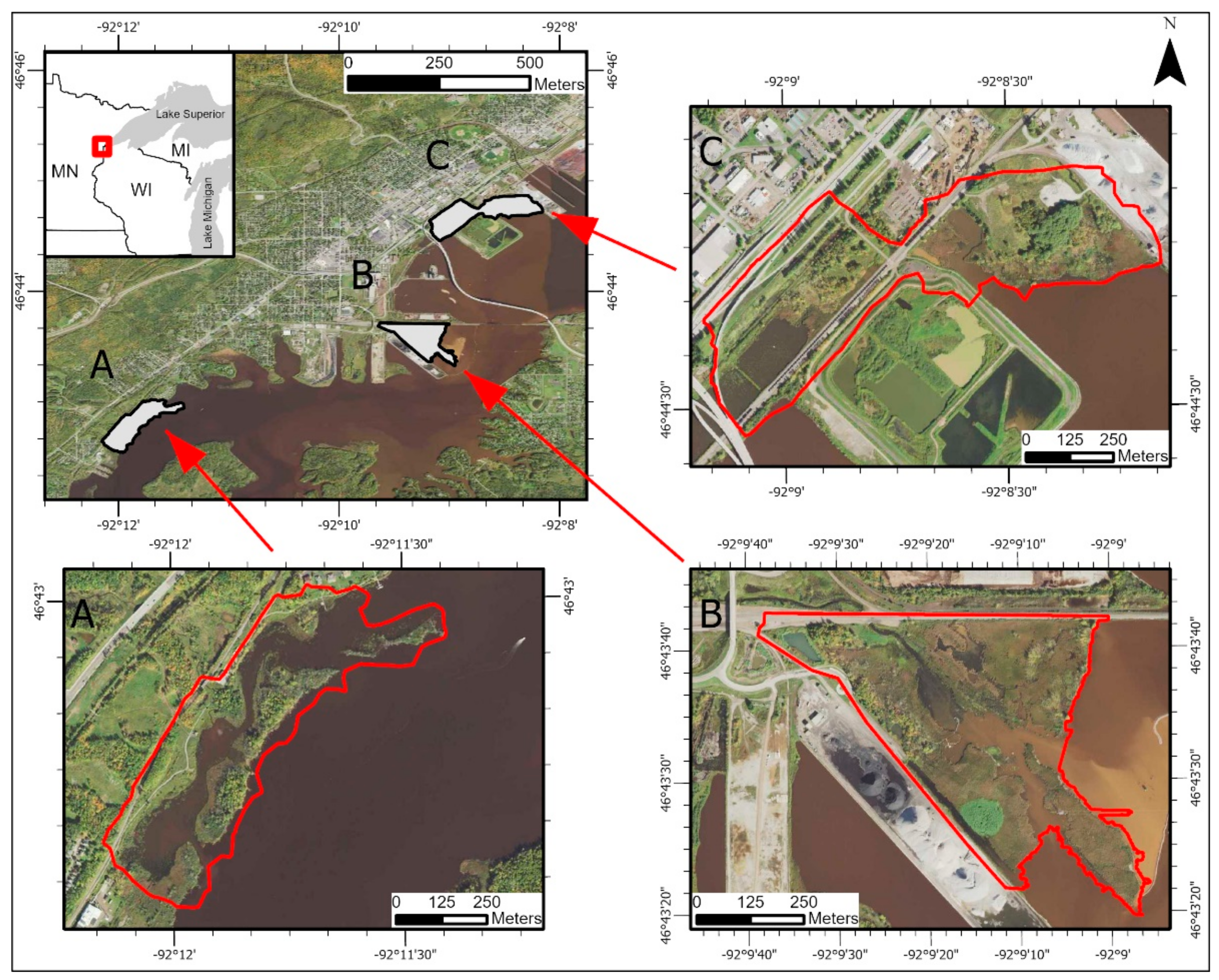
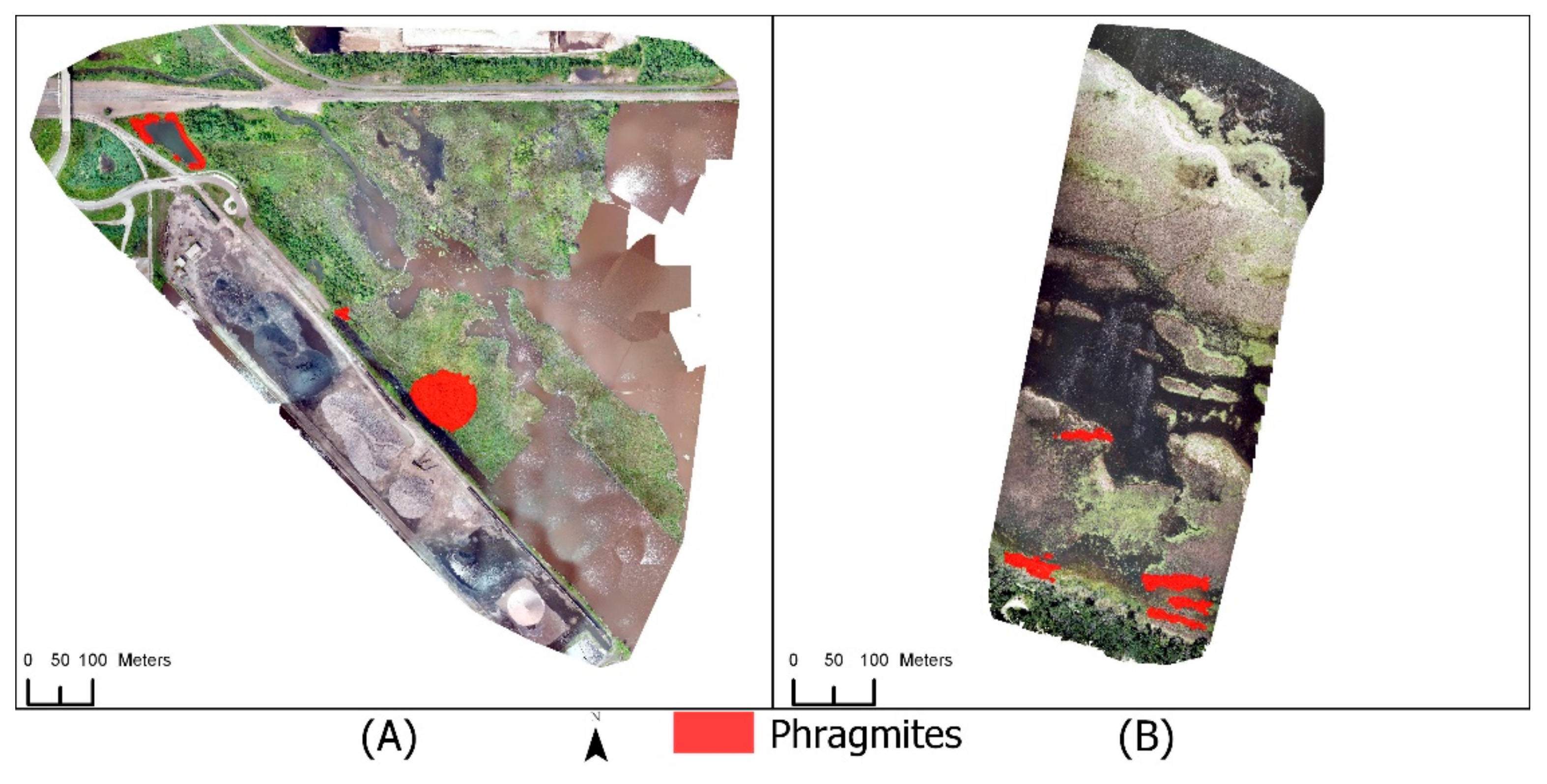
This study aimed to explore the capability of UAS for identifying Phragmites in Minnesota and Michigan using object-based image analysis. The impact of incorporating a CHM and SAR imagery within the classification was also explored. In this text, a CHM is used interchangeably with a normalized digital surface model (nDSM), and it is created by subtracting a digital elevation model (DEM) from a digital surface model (DSM). CHMs can be derived from lidar, SAR, and optical imagery. This study examined the use of both UAS-derived CHMs and stereo satellite-derived CHMs. We aimed to determine the effect of CHMs and SAR backscatter when identifying Phragmites from UAS imagery. The objectives of this study were: (i) determine whether Phragmites can be identified using only the spectral and textural information from three-band (i.e., red, green, and blue; RGB) UAS imagery; (ii) explore the effects of the addition of a canopy height model within the classification, both UAS-derived and stereo satellite-derived; (iii) evaluate whether the addition of SAR backscatter information improves the identification accuracy of Phragmites.
4. Discussion
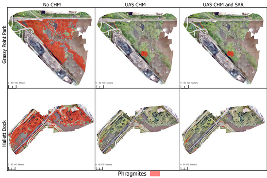
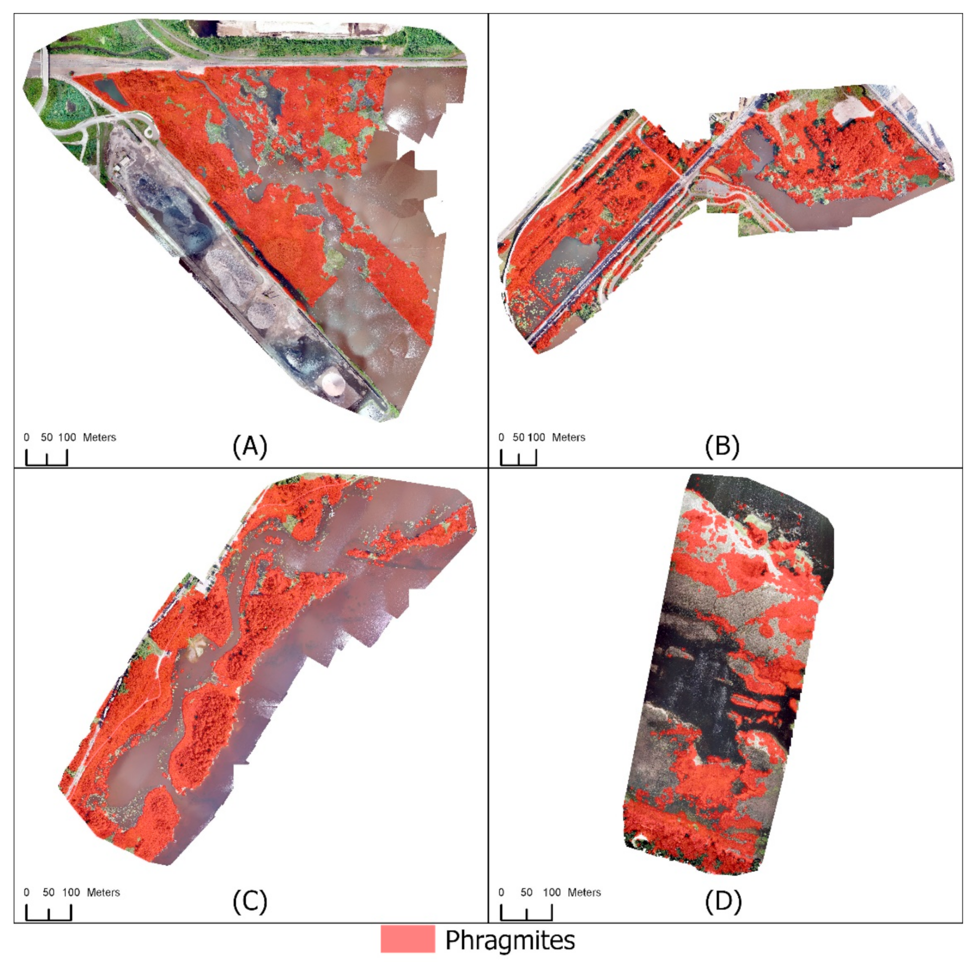
This study used OBIA to identify Phragmites from three-band UAS imagery and tested the functionality of CHMs and SAR within those classifications. Based on the results in four study locations, accurate identification of Phragmites from UAS imagery is unlikely without the use of a CHM. This is clearly demonstrated by the low producer’s and user’s accuracies of the Phragmites class when not using a CHM. Visual analysis of the resulting classifications showed that trees, shrubs, and Typha spp. were highly subject to commission errors in each of the four study sites. Phragmites in the training location exhibited rough textures due to shadowing, which corresponds to low GLCM homogeneity values. Misclassification of woody vegetation and Typha spp. may be due to their similar textural values as Phragmites.
4.1. Use of CHMs for Phragmites Identification
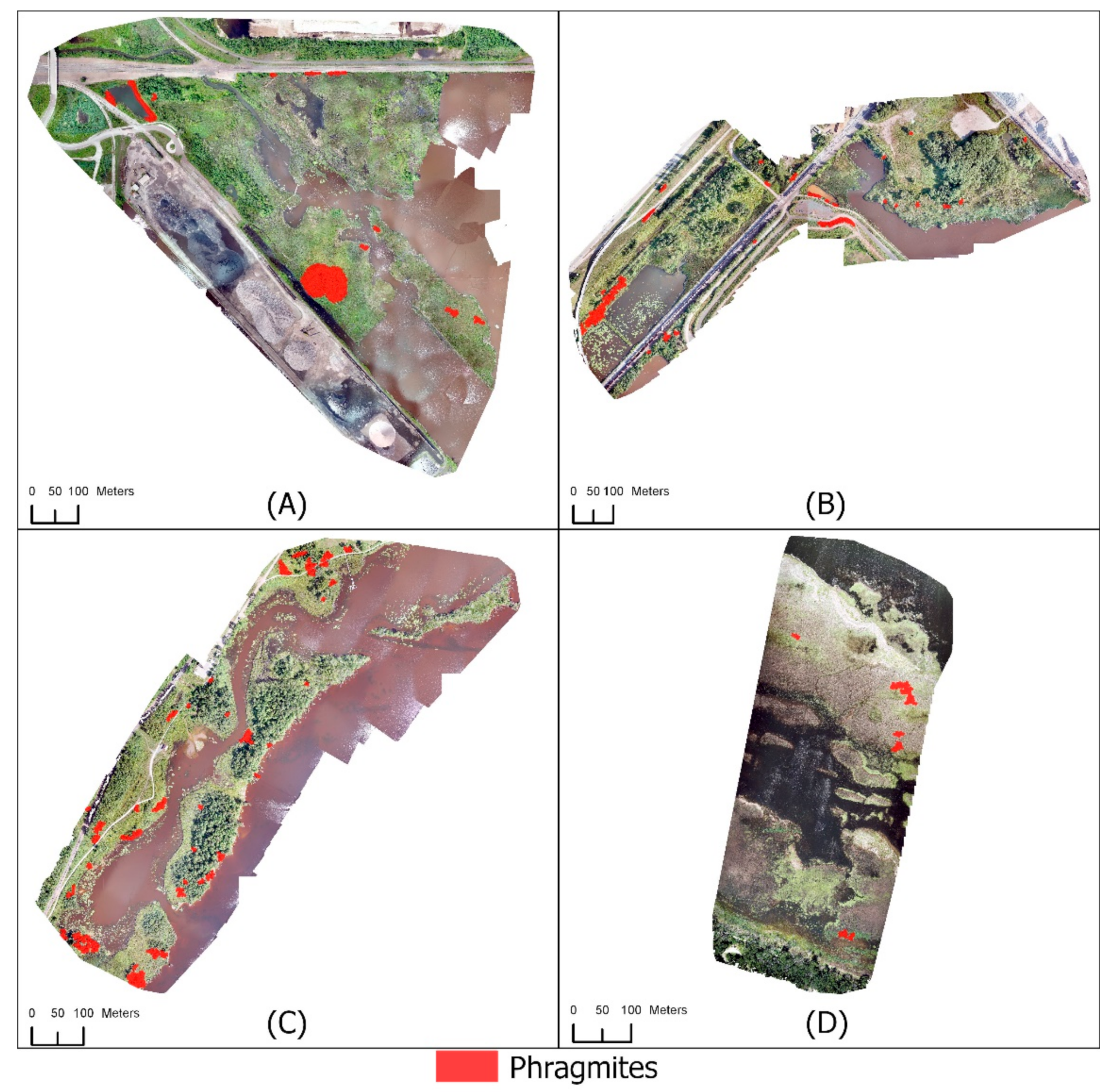
Inclusion of a CHM allowed for a significant increase (>20%) in classification accuracy for three of the four study sites. The increased accuracy is attributed to the exclusion of wetland trees, shrubs, and shorter wetland vegetation from the final Phragmites class. It is possible that the CHM had further impacts. The CHM was used with the RGB imagery when calculating GLCM homogeneity and contrast. Texture values of objects changed, which resulted in objects being included or excluded from the final Phragmites class. Although the separation of vegetation by height resulted in the most significant change to classifications using a CHM, the texture values calculated with the addition of a CHM were important for the classification and refinement of Phragmites objects. In comparison, using texture without a CHM resulted in broad misclassification. Further research is needed to determine the role of textural algorithms for Phragmites classification.
Although the inclusion of a CHM provided a large increase in classification accuracy in three study sites, results from the Saginaw Bay study site demonstrate that classification accuracy is tied to the quality of the CHM. Each study site was flown without ground control points while using single-frequency GNSS equipment. Errors in positional estimates of the UAS will propagate through the workflow, lowering the accuracy of the subsequent UAS data.
Phragmites frequently invades locations where ground control points are difficult to establish. A UAS with post-processing kinematic (PPK) or real-time kinematic (RTK) capabilities would increase positional accuracy [
79,
80,
81] and decrease CHM errors. CHM accuracy is also dependent on the quality of the lidar used to create the DEM. Density of
Phragmites patches may inhibit the lidar laser pulse from striking the ground or water surface below, resulting in returns being incorrectly classified (i.e., vegetation returns classified as ground returns). This issue may be circumvented where
Phragmites is growing as emergent vegetation. A single parameter, mean water level, for example, could be used to create the CHM. However, this method would not be appropriate elsewhere. More testing is needed to determine how to achieve accurate DEMs in locations that
Phragmites invades, as well as the impact of a PPK or RTK enabled UAS on classification accuracy.
The results seen at Saginaw Bay were attributed to the potential CHM errors described above. Portions of live and dead Phragmites stands can be seen in the lidar DEM. Additionally, the GNSS instruments on the DJI Mavic Pro may not be accurate enough for estimating emergent vegetation height. Visual assessment of the UAS-derived DSM showed significant underestimation of vegetation height. This was present even when accounting for potential errors in the lidar-derived DEM. For example, most vegetation was estimated to be under one meter tall. More research is needed to confirm whether a DJI Mavic Pro can accurately estimate the height of Phragmites and non-Phragmites herbaceous vegetation.
Field conditions and Phragmites patch characteristics during data acquisition are another critical aspect to CHM quality. The density of a Phragmites patch directly determines what can be captured in the CHM. The potential to capture individual stalks of Phragmites in a CHM is unlikely. This is due to the increased difficulty of point matching at the top of a Phragmites stalk because of its small size and frequent movement in wind. Higher density Phragmites patches provide more options for point matching, which will lead to a more accurate CHM. The potential issues with proper point matching can be compounded during flooded conditions due to the movement of water. Future research should prioritize methods, data, and field conditions that produce high-quality CHMs.
Satellite-derived CHMs had classification accuracies that were slightly lower than the UAS-derived CHMs. Saginaw Bay was the only study area that had a higher classification accuracy with the satellite-derived CHM than the UAS-derived CHM, but this is attributed to the accuracy of the GNSS equipment on the DJI Mavic Pro. Commission errors were more abundant at the boundaries of tree lines and low vegetation than when using a UAS-derived CHM. This is attributed to the lower spatial resolution of the satellite-derived CHMs. Larger pixel size inhibits a distinct boundary between the tree canopy and low vegetation canopy. Additionally, commission errors may be attributed to the vertical accuracy and adjustment method of the satellite-derived CHMs. Others have noted errors of multiple meters when using commercial satellite stereo retrievals to estimate canopy height [
82,
83,
84]. Errors of this magnitude will directly impact the detection of
Phragmites. Examples of this error can be seen in both the Hallett Dock and Tallas Island study sites. Large sections of herbaceous vegetation were correctly classified in these two sites when using a UAS-derived CHM, but the same areas were incorrectly classified when using a satellite-derived CHM. This issue highlights the need for the evaluation of DSMs created using the SETSM algorithm.
Implications of large-area
Phragmites identification is promising despite the commission errors when using a satellite-derived CHM. Knowing that a CHM is necessary for accurate
Phragmites identification, a major issue with large-area identification is having a CHM from the same growing season as the optical imagery.
Phragmites patches can expand rapidly during a growing season [
85], new patches can establish between years, and active management can reduce patch size and change patch shape. Outdated CHMs would result in inaccurate classifications, potentially causing unaccounted or incorrectly identified
Phragmites patches. These errors could lead to mismanagement of resources apportioned to control
Phragmites. Large-area lidar acquisitions are infrequent, and vegetation structure and abundance will change after the acquisition. Satellite-derived CHMs allow for classifications to use CHMs from the same day as the optical imagery. In addition to up-to-date CHMs, optical satellites frequently collect more than just the RBG spectral bands, which will assist in the discrimination of vegetation [
86]. Large-area identification of
Phragmites using satellite-derived CHMs is the subject of our ongoing studies.
4.2. SAR for Phragmites Identification
Use of the RADARSAT-2 HH polarization did not improve classification accuracy at any of the four study sites. These results are similar to Millard and Richardson (2013) [
87] who found no improvement when pairing SAR with lidar derivatives for wetland classification. Tallas Island and Hallett Dock had no increase in accuracy or decrease in commission errors when incorporating the HH polarization. Commission errors at Grassy Point were reduced to only three objects being misclassified as
Phragmites. Contrarily, omission errors were significantly higher in Saginaw Bay where no
Phragmites was correctly identified. This is attributed to different environmental conditions in the St. Louis River Estuary and Lake Huron. However, these environmental conditions, which are not exclusive to Saginaw Bay, could be present in wetlands in any location. Higher σ° values were detected in the Saginaw Bay study site compared to the other study sites. A majority of the vegetation in Saginaw Bay was flooded, while the vegetation in the Minnesota study sites was not. The HH polarization is more sensitive to double-bounce scattering, and flooded, tall vegetation facilitates double-bounce scattering with perpendicular water-stem surfaces [
32]. Although the CHM caused most omission errors in Saginaw Bay, the failure of the classifier in Saginaw Bay when incorporating the HH polarization was caused by the omission of
Phragmites patches due to higher HH backscatter. The differences between Grassy Point and Saginaw Bay show that environmental conditions have great influence over SAR backscatter. The dielectric properties of all scattering surfaces and the geometry of those surfaces determines the intensity and polarization of the returned signal [
33]. Future work should normalize SAR variables to account for environmental differences between locations.
Results from including the HH polarization demonstrate that using a single polarization from a single date is not effective for differentiating
Phragmites from other wetland vegetation. Different SAR methods than those used in this study may prove beneficial for
Phragmites mapping. For example, others have employed multiple dates of SAR imagery when identifying
Phragmites [
26,
88]. A multi-temporal approach may provide the ability to track changes in wetland vegetation structure across the growing season.
Phragmites has more aboveground biomass than other wetland species [
89,
90] and fast rates of growth [
5]. A multi-temporal approach could differentiate
Phragmites from other species due to seasonal growth characteristics. Others have used polarimetric SAR (PolSAR) to identify different wetland types [
91,
92,
93]. PolSAR decompositions are suitable for differentiating surface features based on their scattering behaviors [
94].
Phragmites may have unique scattering characteristics relative to other wetland vegetation due to its density of stems, large amount of aboveground biomass, and the orientation of large, overlapping leaves. Further testing is needed to determine whether other SAR methods can improve the classification accuracy of
Phragmites.
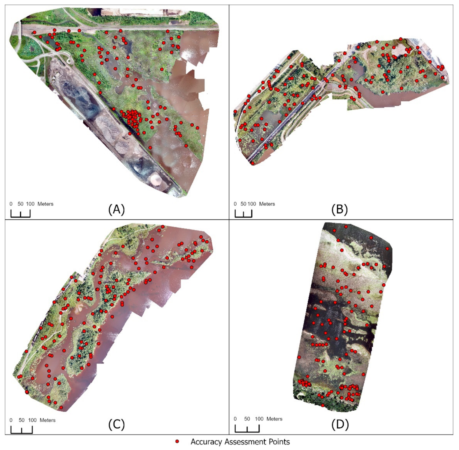
4.3. Validation
Validation of this study was done entirely through visual interpretation of the UAS imagery. Physical mapping of the St. Louis River Estuary had been completed by the GLIFWC, and other individuals provided point data on the location of known Phragmites populations, but the randomized assessment points were not physically validated. Physical validation of each assessment point would allow for higher confidence in the accuracy of each point. Furthermore, the number of Phragmites validation points in Grassy Point Park and Saginaw Bay was low, which likely reduced the precision at which class accuracies could be calculated. The size and shape of the Phragmites patches in the two study areas was not conducive for the creation of more validation points. A higher point density could have been generated, but the generally narrow shape would result in validation points being located too closely together. This brings into question how validation should be completed for classifications where the aim is to identify a cover class that covers a very small percentage of an already small study area. For invasive species mapping, this problem is especially relevant because a land manager’s goal is to identify invasive species’ extent before it becomes too costly to manage, i.e., when populations are small. Further research is needed to determine best practices for this unique problem.


