
Neighboring Discriminant Component Analysis for Asteroid Spectrum Classification


1
Faculty of Information Technology, Macau University of Science and Technology, Taipa, Macau 999078, China
2
State Key Laboratory of Lunar and Planetary Sciences, Macau University of Science and Technology, Taipa, Macau 999078, China
3
School of Communication and Information Engineering, Chongqing University of Posts and Telecommunications, Chongqing 400065, China
4
Global Information and Telecommunication Institute, Waseda University, Tokyo 169-8050, Japan
*
Author to whom correspondence should be addressed.
Remote Sens. 2021, 13(16), 3306; https://0-doi-org.brum.beds.ac.uk/10.3390/rs13163306
Submission received: 1 July 2021
/
Revised: 15 August 2021
/
Accepted: 16 August 2021
/
Published: 20 August 2021
(This article belongs to the Special Issue Recent Advances in Hyperspectral Image Processing)
Abstract
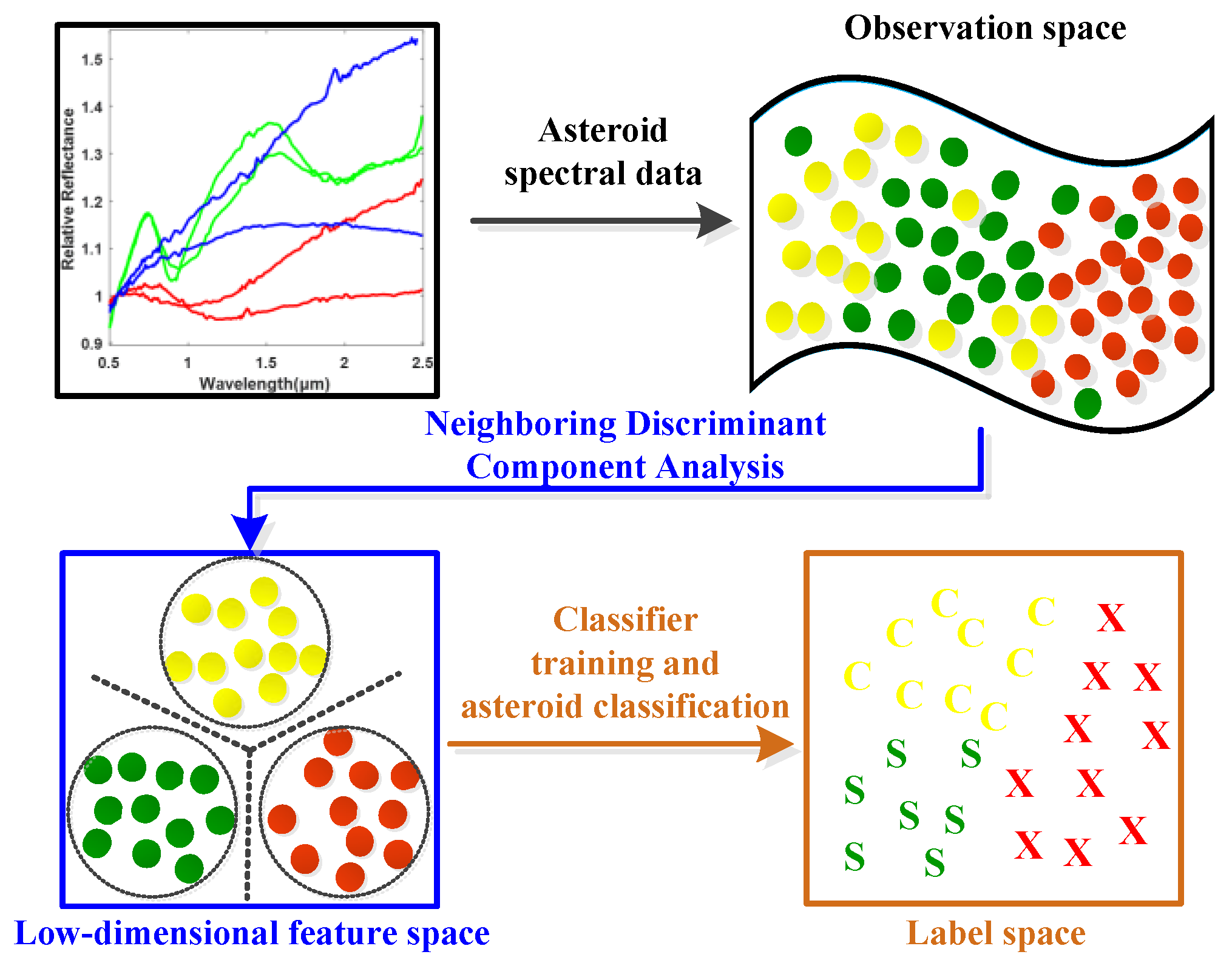
:With the rapid development of aeronautic and deep space exploration technologies, a large number of high-resolution asteroid spectral data have been gathered, which can provide diagnostic information for identifying different categories of asteroids as well as their surface composition and mineralogical properties. However, owing to the noise of observation systems and the ever-changing external observation environments, the observed asteroid spectral data always contain noise and outliers exhibiting indivisible pattern characteristics, which will bring great challenges to the precise classification of asteroids. In order to alleviate the problem and to improve the separability and classification accuracy for different kinds of asteroids, this paper presents a novel Neighboring Discriminant Component Analysis (NDCA) model for asteroid spectrum feature learning. The key motivation is to transform the asteroid spectral data from the observation space into a feature subspace wherein the negative effects of outliers and noise will be minimized while the key category-related valuable knowledge in asteroid spectral data can be well explored. The effectiveness of the proposed NDCA model is verified on real-world asteroid reflectance spectra measured over the wavelength range from 0.45 to 2.45 μm, and promising classification performance has been achieved by the NDCA model in combination with different classifier models, such as the nearest neighbor (NN), support vector machine (SVM) and extreme learning machine (ELM).
1. Introduction
Deep space exploration is the focus of space activities around the world, which aims to explore the mysteries of the universe, search for extraterrestrial life and acquire new knowledge [1,2,3]. Planetary science plays an increasingly important role in the high-quality and sustainable development of deep space exploration [4,5]. Asteroids, as a kind of special celestial body revolving around the sun, are of great scientific significance for human beings in studying the origin and evolution of the solar system, exploring the mineral resources and protecting the safety of the earth due to their large number, different individual characteristics and special orbits [6,7,8]. Studies have shown that the thermal radiation from asteroids mainly depends on its size, shape, albedo, thermal inertia and roughness of the surface [9,10]. The asteroids with different types (such as the S-type, V-type, etc.) in different regions (such as the Jupiter trojans, Hungarian group, etc.) show different spectral characteristics, which establishes the foundations for identifying different kinds of asteroids via remote spectral observation [11,12]. For example, the near-infrared data can reveal the diagnostic compositional information, and the salient features at 1 and 2 μm bands can be used to indicate the existence or absence of olivine and pyroxene [12]. The astronomers have developed many remote observation methods for asteroids, such as spectral and polychromatic photometry, infrared and radio radiation methods [13,14,15,16]. Thus, a large volume of asteroid visible and near-infrared spectral data has been collected with the development of space and ground-based telescope observation technologies, which induced great progress in the field of asteroid taxonomy through their spectral characteristics [17,18,19,20].
The Eight-Color Asteroid Survey (ECAS) is the most remarkable ground-based asteroid observation survey, which gathered the spectrophotometric observations of about 600 large asteroids [14]. However, very few small main-belt asteroids have been observed due to their faintness. With the appearance of charge-coupled device (CCD), it has been possible to study the large-scale spectral data of small main-belt asteroids with a diameter less than 1 km [21]. The first phase of the Small Main belt Asteroid Spectroscopic Survey (SMASSI) was implemented from 1991 to 1993 at the Michigan-Dartmouth-MIT Observatory [15,20]. The main objective of SMASSI was to measure the spectral properties for small and medium-sized asteroids, and it primarily focuses on the objects in the inner main belt aiming to study the correlations between meteorites and asteroids. Based on the survey, abundant spectral measurements for 316 different asteroids have been collected. In view of the successes of SMASSI, the second phase of the Small Main-belt Asteroid Spectroscopic Survey (SMASSII) mainly focused on gathering an even larger and internally consistent asteroid dataset with spectral observations and reductions, which were carried out as consistently as possible [20]. Thus, SMASSII has provided a new basis for studying the composition and structure of the asteroid belt [9].
For asteroid taxonomy, Tholen et al. applied the minimal tree method by a combination with the principal component analysis (PCA) method in order to classify nearly 600 asteroid spectra from the ECAS [14]. For more comprehensive and accurate classification of asteroids, DeMeo et al. developed an extended taxonomy to characterize visible and near -infrared wavelength spectra [20]. The asteroid spectral data used for the taxonomy are based on the reflectance spectral characteristics measured in the wavelength range from 0.45 to 2.45 μm with 379–688 bands. In summary, the dataset was comprised of 371 objects with both visible and near-infrared data. SMASSII dataset provided the most visible wavelength spectra, and the near-infrared spectral measurements from 0.8 to 2.5 μm were obtained by using SpeX, the low-resolution to medium-resolution near-infrared spectrograph and imager at the 3-m NASA IRTF in Mauna Kea, Hawaii [20]. A detailed description for the dataset is illustrated in Table 1. Based on the dataset, DeMeo et al. have presented the taxonomy, as well as the method and rationale, for the class definitions of different kinds of asteroids. Specifically, three main complexes, i.e., S-complex, C-complex and X-complex, were defined based on some empirical spectral characteristics/features, such as the spectral curve slope, absorption bands and so on.
Nevertheless, the question of how to automatically discover the key category-related spectral characteristics/features for different kinds of asteroids remains an open problem [9,22,23]. Meanwhile, owing to the noise of observation systems and the ever-changing external conditions, the observed spectral data usually contain noise and distortions, which will cause spectrum mixture due to the random perturbation of electronic observation devices. As a result, the observed asteroid spectra data often show indivisible pattern characteristics [24,25]. Furthermore, the observed spectral data always have wide bands, such as the visible and near-infrared bands. Thus, the reflectance at one wavelength is usually correlated with the reflectance of the adjacent wavelengths [26]. Accordingly, the adjacent spectral bands are usually redundant, and some bands may not contain discriminant information for asteroid classification. Moreover, the abundant spectral information will result in high data dimensionality containing useless or even harmful information and bring about the “curse of dimensionality” problem, i.e., under a fixed and limited number of training samples, the classification accuracy of spectral data might decrease when the dimensionality of spectral feature increases [27]. Therefore, it is necessary to develop effective low-dimensional asteroid spectral feature learning methods and find the latent key discriminative knowledge for different kinds of asteroids, which will be very beneficial for the precise classification of asteroids.
Machine learning techniques have developed rapidly in recent years for spectral data processing and applications, such as the classification and target detection [28,29,30,31,32,33,34,35]. For example, the classic PCA has been applied to extract meaningful features from the observed spectral data without using the prior label information. PCA is also useful for asteroid and meteorite spectra analysis due to the fact that many of the variables, i.e., the reflectance at different wavelengths, are highly correlated [15,20,36]. Linear discriminant analysis (LDA) can make full use of the label priors by concurrently minimizing the within-class scatter and maximizing the between-class scatter in a dimension-reduced subspace [37]. In addition to the above statistics-based methods, some geometry theory-based methods have also been proposed for the problem of data dimensionality reduction. For example, the locality preserving projections (LPP) assume that neighboring samples are likely to share similar labels, and the affinity relationships among samples should be preserved in subspace learning/dimension reduction [38]. Locality preserving discriminant projections (LPDP) have also been developed with locality and Fisher criterions, which can be seen as a combination of LDA and LPP [39,40].
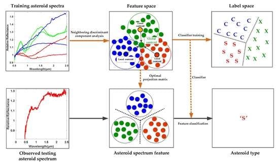
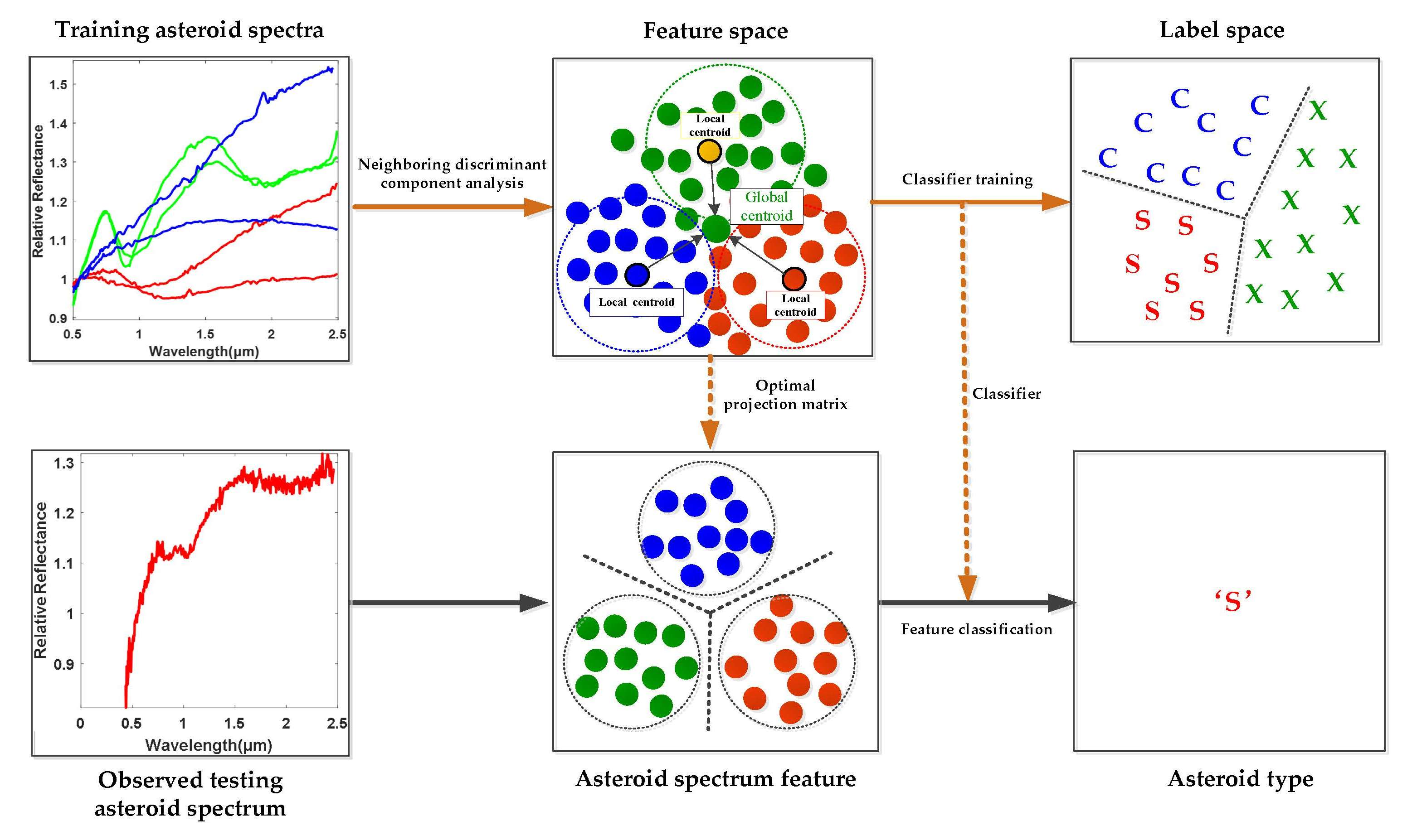
In order to define the class boundaries for asteroid classification, traditional methods always empirically determine the spectral features by relying on the presence or absence of specific features, such as the spectral curve slope, absorption wavelengths and so on, which might be intricate and less reliable. Based on the well labeled asteroid spectral dataset described in Table 1 the main objective of this paper is to study the pattern characteristics of different categories of asteroids from the perspective of data-driven machine learning technique and to develop efficient asteroid spectral feature learning and classification method in a supervised fashion, as shown in Figure 1. In order to be specific, it is assumed that not only the specified absorption bands, such as the 1 μm and 2 μm bands but also all the spectral wavelengths might carry some useful diagnostic information for asteroid category identification and will contribute to the accurate classification of different kinds of asteroids. As a result, the spectral data spanning across the visible to near-infrared wavelengths, i.e., from 0.45 to 2.45 μm, are treated as a whole in order to automatically discover the key category-related discriminative information for efficient asteroid spectral feature learning and classification by using supervised data-driven machine learning methodology. The novelties and contributions of this paper are summarized as below.
- (1)
- Instead of empirically determining the spectral features via the presence or absence of specific spectral features to define asteroid class boundaries for classification, this paper presents a novel supervised Neighboring Discriminant Components Analysis (NDCA) model for discriminative asteroid spectral feature learning by simultaneously maximizing the neighboring between-class scatter and data variances, minimizing the neighboring within-class scatter to alleviate the overfitting problem caused by outliers and enhancing the discrimination and generalization ability of the model.
- (2)
- With the neighboring discrimination learning strategy, the proposed NDCA model has stronger robustness to abnormal samples and outliers, and the generalization performance can thus be improved. In addition, the NDCA model transforms the data from the observation space into a more separable subspace, and the key category-related knowledge can be well discovered and preserved for different classes of asteroids with neighboring structure preservation and label prior guidance.
- (3)
- The performance of the proposed NDCA model is verified on real-world asteroid dataset covering the spectral wavelengths from 0.45 to 2.45 μm by combining with different baseline classifier models, including the nearest neighbor (NN), support vector machine (SVM) and extreme learning machine (ELM). In particular, the best result is achieved by ELM, with a classification accuracy of about 95.19%.
The reminder of this paper is structured as follows. Section 2 introduces related works on subspace learning/dimension reduction and machine learning classifier models. The proposed NDCA model is meticulously introduced in Section 3. Section 4 contains the experimental results and discussions. The final conclusion is given in Section 5.
2. Related Work
2.1. Notations Used in This Paper
In this paper, the observed asteroid visible and near-infrared spectroscopy dataset is denoted as comprising spectral samples with dimensionality from classes. is the number of the samples in the i-th class. The label matrix for is denoted as with as the label vector for . The label of each sample in is coded as a C-dimensional vector, and the j-th entry of is +1 with the remaining entities as 0, which indicates that sample belongs to the j-th category. The basic idea of linear low-dimensional feature learning, i.e., dimension reduction, is to automatically learn an optimal transformation matrix with d < D, which can project the observed spectral data from the original high D-dimensional observation space into a lower d-dimensional feature subspace, and obtains the low-dimensional meaningful features of via . Table 2 summarizes the important notations used in this paper.
2.2. Low-Dimensional Feature Learning for Spectral Data
In the process of low-dimensional feature learning, the key data knowledge and information, such as the discriminative structures, should be preserved and enhanced. Meanwhile, the noise and redundant information should be removed and suppressed. Principal component analysis (PCA) is a widely applied unsupervised statistical dimension reduction and feature learning method, which focuses on maximizing the variance of the data with significant principal components [33]. A formulation for PCA can be derived by solving the following least squares problem:
where means the Frobenius norm of a matrix, and is an identity matrix with the size of . Formula (1) is equivalent to maximizing the variance of the transformed data as follows [33].
Unlike PCA, LDA is a supervised dimension reduction learning method and aims to maximize the separability between different classes and enhance the compactness within each class with the guidance of label information as described below [34,41,42,43]:
where and are, respectively, the within-class and between-class scatter matrices of data, which are calculated in the following way [34,41,42,43]:
where is the j-th sample of the i-th class, and and are the mean value of the samples in i-th class and all the samples in , respectively.
2.3. Classifier Models for Spectral Data Classification
Classifier models, such as NN, SVM [44] and ELM [45,46,47,48], have been commonly used in the contexts of machine learning and pattern recognition communities in order to recognize and classify spectral data. In particular, the extreme learning machine (ELM) is a newly developed machine learning paradigm for the generalized single hidden layer feed forward neural networks and has been widely studied and applied due to its some unique characteristics, such as the high learning speed, good generalization and universal approximation abilities [47]. The most noteworthy characteristic for ELM is that the weights between the input and the hidden layers are randomly generated without further adjustments. The objective function of ELM is formulated as below:
where denotes the output weights connecting the hidden layer and the output layer. is the prediction error matrix with respect to the training data. is the hidden layer output matrix and is computed with the following method:
where is the activation function in the hidden layer, for example the sigmoid function. and refer to the randomly generated input weights and bias, respectively. The output weight matrix is used to transform the data from the L-dimensional hidden layer space into the C-dimensional high-level label space and is analytically calculated in the following manner.
With the optimal output weight matrix obtained, the predicted label for a new test sample can be computed as follows:
where is the hidden layer output for test sample .
3. The Proposed Neighboring Discriminant Component Analysis Model: Formulation and Optimization
The remote observed asteroid spectral data usually contain noise and outliers, which will mix different categories of asteroids and make them inseparable. In addition, learning with outliers will easily cause overfitting problem, which will decrease the generalization ability of machine learning models for testing samples. Thus, the key problem is to distinguish the outliers and to select the most valuable samples for the learning of low-dimensional feature subspace and preserve the key discriminative data knowledge for different classes of asteroids.
To this end, the idea of neighboring learning is introduced to find a neighboring group of valuable samples from all the training samples as well as the samples in each class, and the outliers and noised samples are excluded in dimension reduction learning in order to enhance the generalization ability of the model. As shown in Figure 2, the normalized asteroid spectral data are firstly inputted as in (a). Secondly, (b) finds the neighboring samples in each asteroid class in order to characterize the neighboring within-class and between-class properties of data. Meanwhile, the neighboring samples from all the samples for neighboring principal components were found to preserve the most valuable data information as in (c). With the basic principles of (b) and (c), a clearer class boundary can be found to alleviate the overfitting problem caused by the outliers and noised samples and enhance the neighboring and discriminative information of data for efficient spectral feature learning shown in (d). In order to achieve this goal, the neighboring between-class and within-class scatter matrices need to be calculated in order to characterize the neighboring discriminative properties of the observed asteroid spectra.
Neighboring between-class scatter matrix computation: Firstly, calculate the global centroid for all the samples in training dataset and find Nb = Rb · N neighboring samples to by using between-class neighboring ratio Rb (0 < Rb < 1). Thus, Nb = [Nb1, Nb2, …, Nbc, …, NbC] global neighboring samples can be obtained with Nbc as the number of the neighboring samples in the c-th class for computing the neighboring between-class scatter matrix. Secondly, compute the local centroid for the c-th class, and is the j-th sample in the c-th class of the neighboring samples . Finally, the neighboring between-class scatter matrix is calculated as follows.
At the same time, the global neighboring samples are used to calculate the covariance matrix as below.
Neighboring within-class scatter matrix computation: Firstly, calculate the basic local centroid for each class of samples, where is the i-th sample in the c-th class of , and then find the samples group containing Nwc = Rw · Nc neighboring samples to by using within-class neighboring ratio Rw (0 < Rw < 1) in the i-th class. Secondly, refine the local centroid of each class using the samples in the obtained neighboring group of samples . Finally, compute the neighboring within-class scatter matrix as follows:
where is the refined centroid of each class based on the neighboring sample groups , and is the i-th samples of c-th class samples in the neighboring group. By comprehensively consider Equations (10)–(12) in a dimension-reduced subspace, the following optimization problem is formulated.
The details for deriving Equation (13) based on Equations (10)–(12) are shown in Appendix A. In Equation (13), γ and μ are the tradeoff parameters for balancing the corresponding components in the objective function, from which one can observe that, in the subspace formed by P, the goals of neighboring between-class scatter maximization, within-class scatter minimization and neighboring principal components preservation can be simultaneously achieved. Accordingly, the side effects of outliers and noised samples will be suppressed to the largest extent. As a result, the global and local neighboring discriminative structures and principal components will be enhanced and preserved by using the neighboring learning mechanism. Furthermore, optimization problem (13) can be transformed into the following one by introducing an equality constraint [49]:
where is a constant used to ensure a unique solution for model (13). The objective function for model (14) can be formulated as the following unconstrained one by introducing the Lagrange multiplier λ.
Then, the partial derivative of the objective function (15) with respect to P is calculated and set as zero, resulting in the following equations:
where the projection matrix can be acquired, which is composed of the eigenvectors corresponding to the first d largest eigenvalues λ1, λ2 …, λd of the eigenvalue decomposition problem as described below.
Once the above optimal projection matrix is calculated, the training data are projected into the subspace using in order to acquire the low-dimensional discriminative feature of the observed spectral data. Afterwards, a classifier model is trained using the dimension-reduced training data. For testing, an asteroid spectral sample with unknown label is firstly transformed into the subspace by using the optimal projection matrix P and then classified by the trained classifier model.
4. Experiments
4.1. Preprocessing for the Asteroid Spectral Data
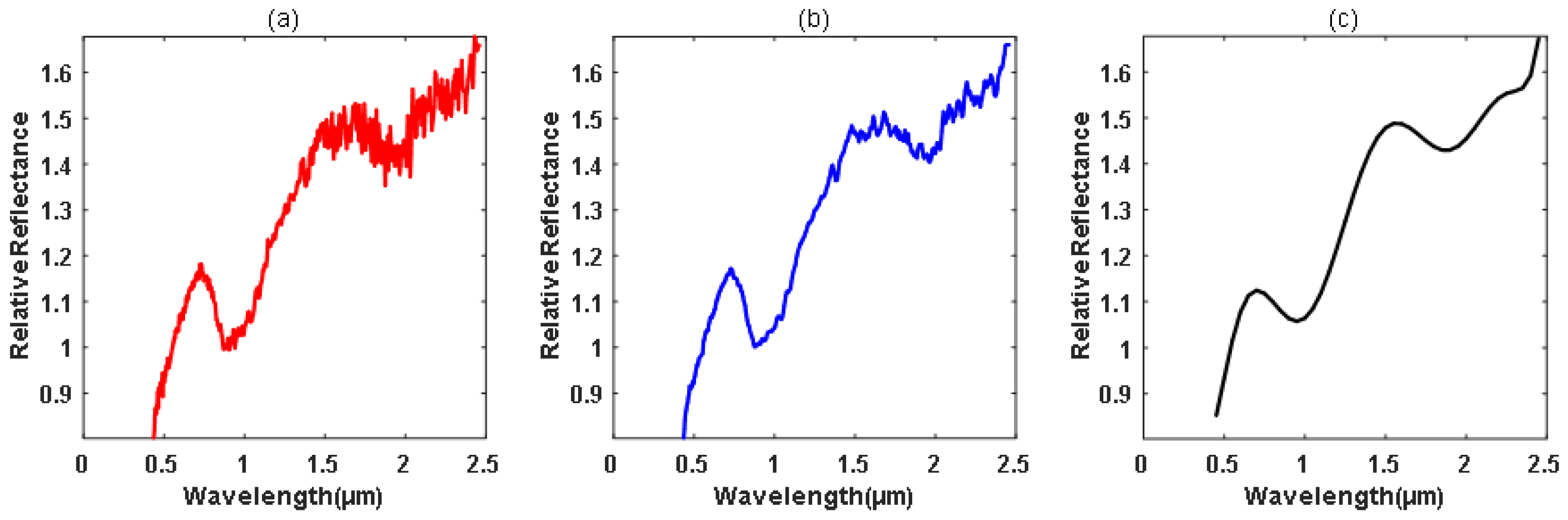
As shown in Table 3, a part of the samples described in Table 1 was used in the study. The data preprocessing was performed to preliminarily reduce the influences of noise for ease of classification. Firstly, the original spectral data were filtered and smoothed by using some data filtering method, such as the moving average filter. Secondly, the discrete spectrum measurements were fitted using the high-order polynomial method. Thirdly, the obtained fitted spectral curves within the spectral wavelengths from 0.45 to 2.45 μm were sampled with certain step interval. Several examples the original spectra, smoothed spectra and the fitted spectra for different kinds of asteroids are shown in Figure 3, Figure 4 and Figure 5, from which one can see that the abnormal noises in some spectral bands were suppressed to a certain extent.
4.2. Experimental Setup and Results
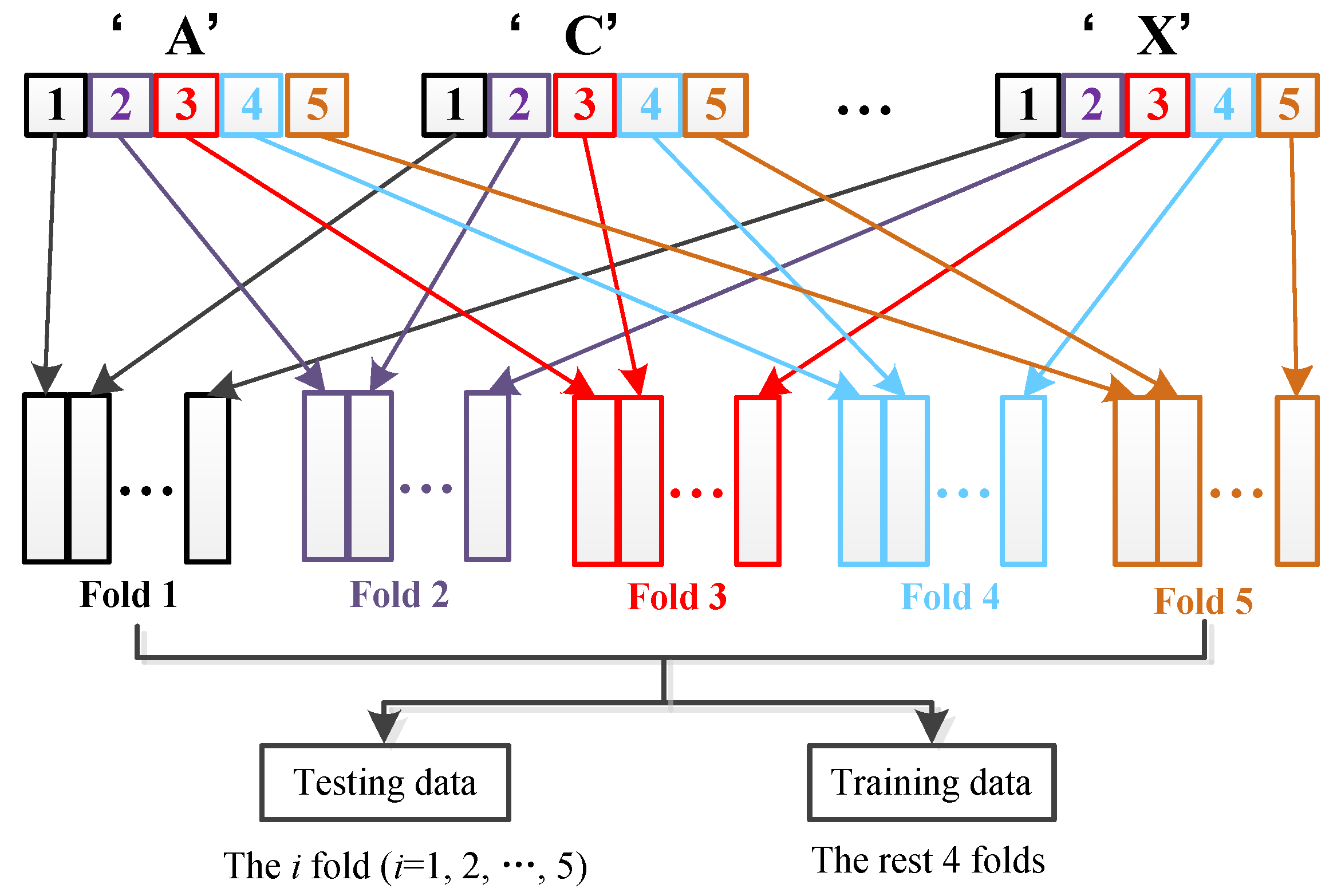
As previously mentioned, the smoothed asteroid spectral curves were fitted using a high order polynomial, which was furthered sampled in wavelength region from 0.45 to 2.45 μm with an increment step interval of 0.05 μm, obtaining 41 measurements for each asteroid spectrum. In order to valid the effectiveness of the proposed method, the data from different classes were firstly approximately equally divided into five groups as shown in Figure 6. Afterwards, the five groups of samples from different classes are merged into 5-folds. Each fold contains five groups of samples with each group from distinct classes. The data partition of the 5-folds was illustrated in Table 4. Then, the 5-fold cross validation (CV) strategy was adopted for the performance evaluation of different methods. Specifically, random 4folds of samples were selected and used as the training dataset, and the remaining 1 fold of samples was utilized for testing; thus, five experiments were carried out. A detailed description for the five experiment settings is shown in Table 5, and the individual and average classification accuracy of different methods on the five experiments will be reported. All the experiments were conducted under the same settings and computing platform. Thus, a fair comparison between different methods can be guaranteed. The proposed NDCA model was compared with several representative subspace learning methods, including PCA, LDA, LPP and LPDP. Moreover, the sampled raw asteroid spectral data without feature learning were also included for comparison. In addition, some baseline classifier models, such as the nearest neighbor (NN), SVM and ELM, were adopted in the experiments for the classification of the asteroid features.
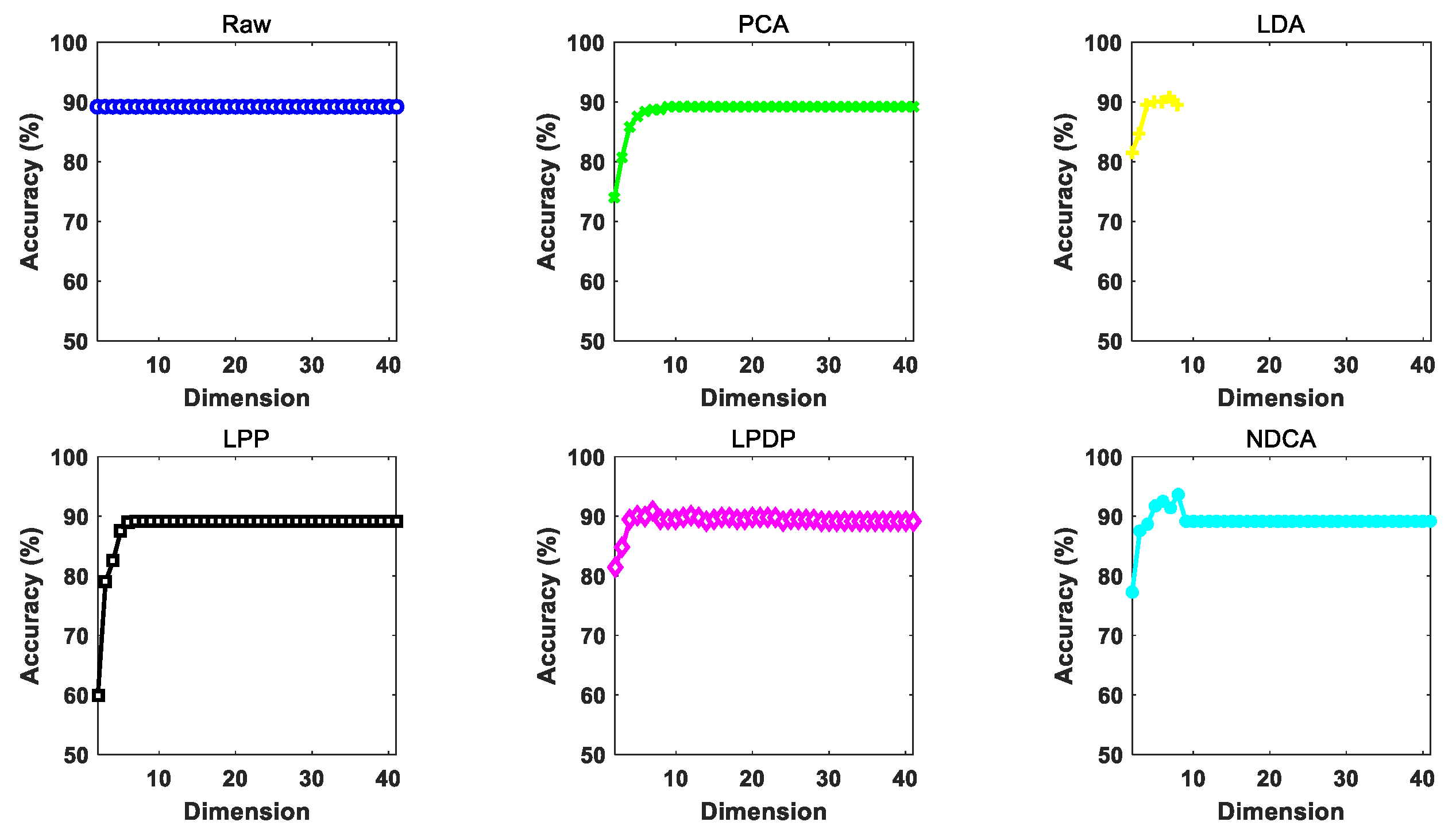
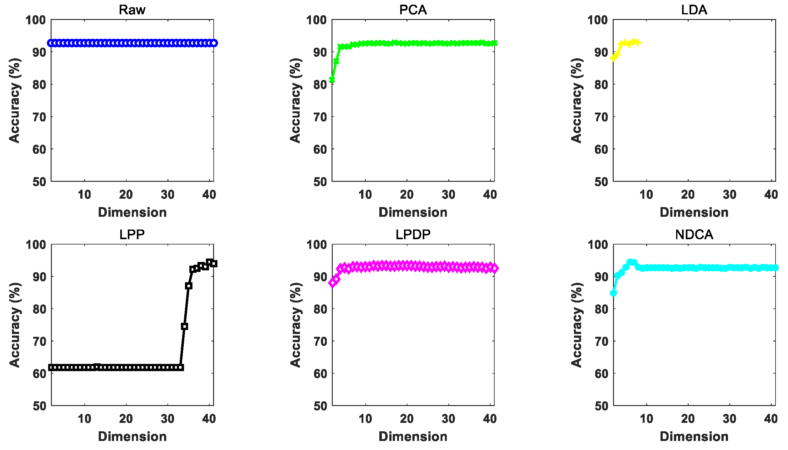
The performance of different dimension reduction methods under gradually increasing reduced dimension d (from 2 to 41 with an interval of 1) by using different baseline classifier models, i.e., NN, SVM and ELM, is illustrated in Figure 7, Figure 8 and Figure 9. In addition, the highest classification accuracy of different comparative methods under varying dimensions for each experiment is reported in Table 6, Table 7 and Table 8, respectively. Based on the experimental results, all the comparative methods tend to achieve improved classification performance with the growth of feature dimension. For the proposed NDCA method, the classification accuracy of NDCA method increases first, then decreases and finally tends to be stable. This could be due to the fact that too many dimension features might introduce redundant harmful information and decrease classification performance. It is also notable that the classification performance of LPP stabilizes first and then increases when the feature dimension increases to about 33 in the case of SVM and ELM. Meanwhile, when LPP combines with the NN classifier, the classification performance increases first and, finally, tends to be stable. Even though LPP can only achieve comparative classification performance in a relatively high dimensionality, the best classification accuracies for LPP in combination with NN, SVM and ELM also reached 89.7565%, 92.8158% and 94.4711%, respectively.
Generally speaking, the proposed NDAC method can yield the best classification accuracies of 94.1971%, 93.6377% and 95.1895% with different classifiers. Table 9 further summarizes the performance improvement of the proposed NDCA method in comparison with different comparative methods by using different classifiers. Specifically, the maximal performance improvement of NDCA method is 4.9886% in comparison with raw feature and the PCA method by using NN as the classifier, and the minimal performance improvement of NDCA method is 0.4521% when comparing with LPDP plus ELM method. In summary, the average performance improvement in all the experimental settings is 2.045%. Therefore, the effectiveness and superiority of the proposed NDCA method can be clearly observed from the perspective of experimental verifications.
In addition, the results show that the raw data without feature learning achieves worse classification performance among all the comparative methods. In contrast, the proposed NDCA model can achieve the highest classification accuracy by combining with different classifier models. Moreover, it should be noted that the highest accuracy can be achieved when the feature dimension is around nine. Thus, the optimal reduced dimension d can be searched around the total number of categories for the samples in asteroid spectral dataset.
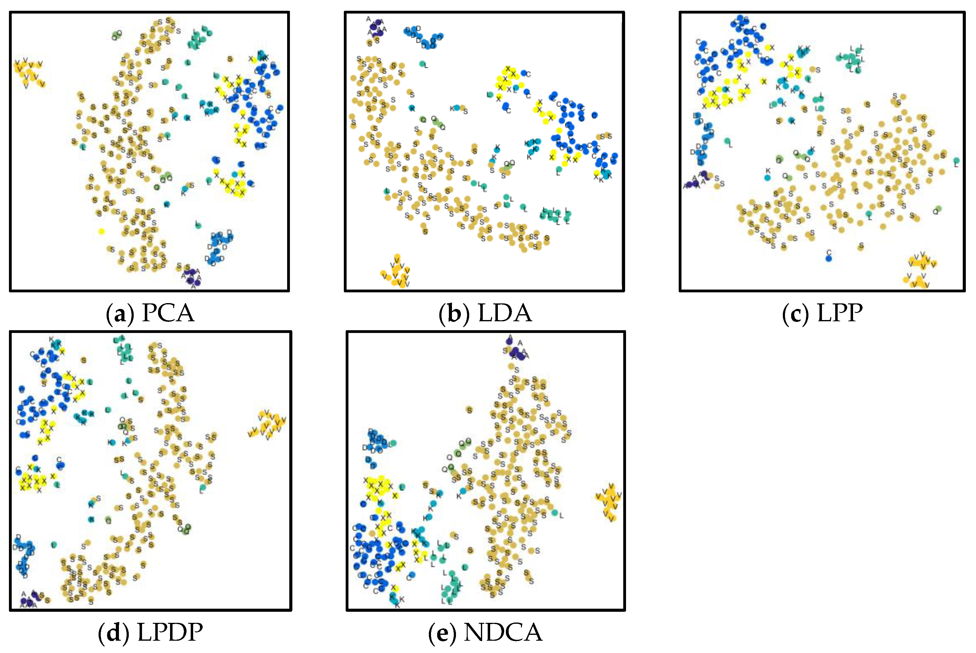
Furthermore, the scatter points for the first two dimensions acquired by different methods are visualized in Figure 10 in order to further intuitively observe the low-dimensional feature learning performance. In contrast, the scatter points obtained by the comparative methods have serious data mixture effects between different classes, especially the “K”, “L” and “Q” classes, which will result in lower classification performance. From Figure 10e, it can be observed that the scatter points derived by the proposed NDCA model show better within-class compactness and between-class separation characteristics with relatively clearer category boundaries. Accordingly, the spectral characteristics within each class and the discriminant between different classes of asteroids are fully explored and enhanced by using the proposed NDCA model. By combining with the off-the-shelf classifier models, the class boundaries between different kinds of asteroid spectral data can be easily found, which will result in promising generalization and classification performance.
4.3. Analysis for NDCA Parameters
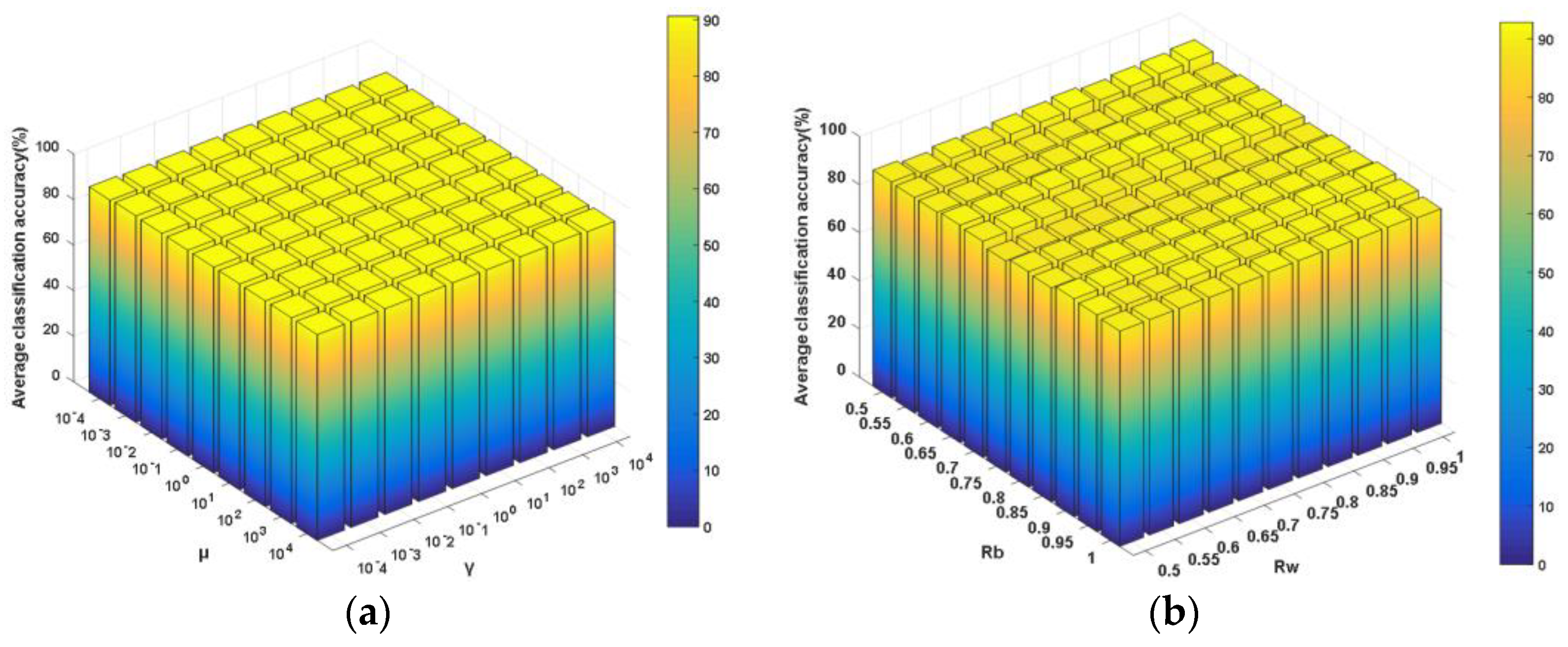
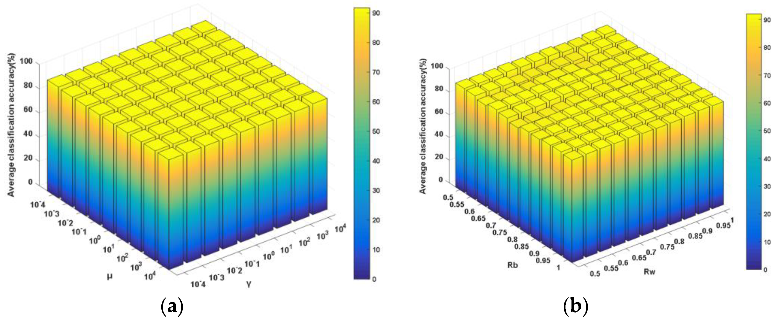
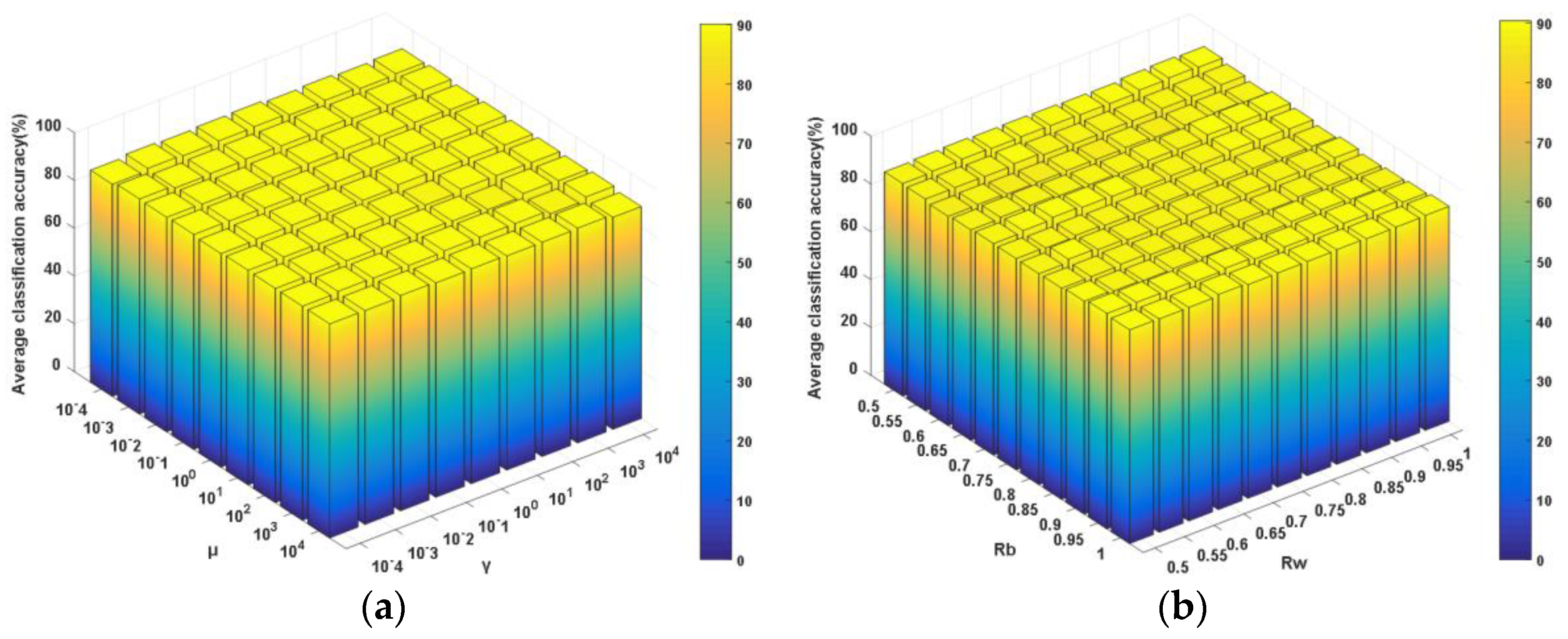
Apart from the dimensionality of the derived feature subspace d, the proposed NDCA model has several key other parameters, including the between-class neighboring ratio Rb, the within-class neighboring ratio Rw and the balance parameters γ and μ in the model formulation (13). Obviously, different parameter settings will result in fluctuating performances. Thus, parameter sensitivity analyses were needed to be conducted in order to show the classification performance variation with respect to these parameters. Specifically, the four parameters were divided into two groups, i.e., (γ, μ) and (Rw, Rb). Among them, γ and μ were selected from the candidate parameter set {10g, g = −4, −3, −2, −1, 0, 1, 2, 3, 4}, while Rw and Rb were selected from the candidate parameter set {0.5, 0.55, 0.6, 0.65, 0.7, 0.75, 0.8, 0.85, 0.9, 0.95, 1}. As shown in Figure 11, Figure 12 and Figure 13, one can observe that the average classification performance change surfaces in sub-figures (a) of Figure 11, Figure 12 and Figure 13 are smoother and more stable within a wide parameter setting range, which means that the classification is not very sensitive to the settings of parameter pair (γ, μ). By contrast, the classification performance changes more acutely with the variations of different parameter pairs (Rw, Rb).
4.4. Analysis for ELM Classifier Parameters
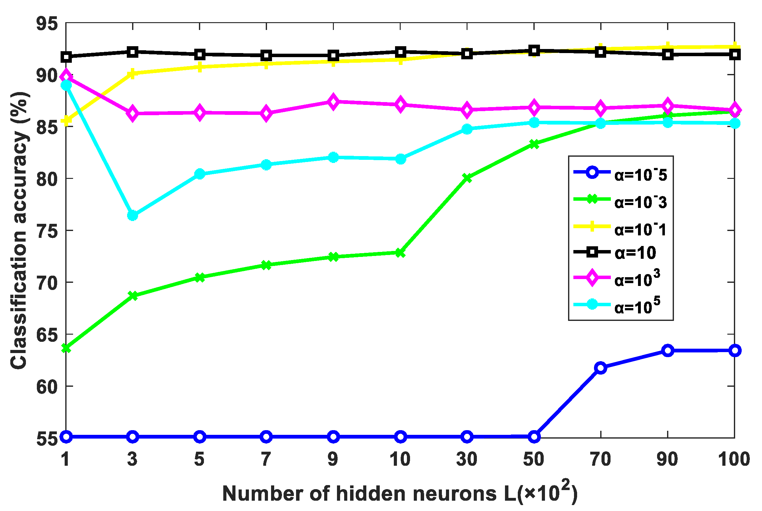
The former experiments show that the proposed NDCA method can generally achieve promising and higher classification accuracy in combination with ELM. As shown in formulation (6), ELM has two key hyper-parameters, i.e., the number of hidden neurons L and the balance parameter α. Figure 14 shows that classification performance changes with different settings of L and α. In general, with the increase in the hidden neurons, the classification accuracy increases first and then tends to be stable. In the experiments, the number of hidden neurons L in ELM is empirically set around 9000. As for the trade-off parameter α, the classification accuracy first improves when α increases from 10−5 to 10 and then degrades when α increases from 10 to 105. In the experiments, α can be set around 10 by which promising performance can be expected.
From the above experimental results, we observe the following:
- (1)
- The benefits of feature learning for asteroid spectrum classification. In the experiments shown in Table 6, Table 7 and Table 8, the original observed raw spectral data without feature learning were directly fed into the classifier models, i.e., NN, SVM and ELM, for classification. The average classification performances achieved by NN, SVM and ELM were 89.2085%, 91.7047% and 92.6963%, respectively, which were generally the worst performance among all the comparative methods. In contrast, the classification performance achieved by the same classifier models after feature learning obtained some improvement. For example, LPP plus NN, SVM and ELM can, respectively, achieve the improved classification accuracies of 89.7565%, 92.8158% and 94.4711%. The results can verify the benefits of feature learning for the improvement of asteroid spectral classification accuracy.
- (2)
- The advantages of the proposed NDCA model. In comparison with several representative low-dimensional feature learning methods, the proposed NDCA model can generally achieve better classification performance by combining with different classifier models. Specifically, NDCA plus NN, SVM and ELM can achieve the highest classification accuracies of 94.1971%, 93.6377% and 95.1895%, respectively. The improvements are mainly due to the following two aspects. Firstly, the NDCA model is a supervised dimension reduction method and inherits the merits of the existing methods, which can fully utilize label knowledge in order to find the key category-related information of spectral data for discriminative asteroid spectral feature learning and classification. Secondly, the introduction of neighboring learning methodology can significantly reduce the side effects of outliers and noised samples in order to alleviate the overfitting problem, which will enhance the robustness of the leant low-dimensional features and finally improve the generalization ability and classification performance of the proposed model in testing.
- (3)
- The superiority of ELM. Three baseline classifier models, including NN, SVM and ELM, were used in the experiments. In particular, the best results are obtained by NDCA plus ELM with a classification accuracy of about 95.19%, which is generally superior to the comparing classifier models. To the best of our knowledge, this work is the first attempt to apply ELM in asteroid spectrum classification, and very competitive performance has been achieved, which can provide new application scenarios and perspectives for ELM community.
- (4)
- Future work discussion. First, future work will consider employing feature selection methods in order to study the asteroid spectral characteristics. Distinct from feature learning/extraction methods, which adopts the idea of data transformation, feature/band selection methods use the idea of selection and aim to automatically select a small subset of representative spectral bands in order to remove spectral redundancy while simultaneously preserving the significant spectral knowledge. Since the feature selection is performed in the original observation space, the specific selected bands have clearer physical meanings with better interpretability. As a result, feature/band selection is an important technique for spectral dimensionality reduction and has room for further improvement. Second, the visualization in Figure 10 for the scatter points of the first two components acquired by different methods showed that some classes of asteroid spectra with limited training samples are seriously mixed and overlapped. One possible reason is that the numbers of training samples from different classes were unbalanced. For example, the number of samples for ‘S’ class asteroid is 199, while the ‘A’ class asteroid only has six samples. When classifying data with complex class distribution, the regular learning algorithm has a natural tendency to favor the majority class by assuming balanced class distribution or equal misclassification cost. As a result, the sample imbalance problem will result in learning bias, and the generalization ability of the obtained model is, thus, restricted. It is significant to deal with the data imbalanced problem and establish balanced data distribution by some sampling or algorithmic methods in future works such that the imbalanced class distribution problem can be well handled and alleviated, which can improve the accuracy of asteroid spectral data analysis.
5. Conclusions
This paper has introduced a novel supervised NDCA learning model for asteroid spectral feature learning and classification. The key idea is to distinguish the outliers and noised samples in order to alleviate the overfitting problem and to find the significant category-related features such that the classification performance can be improved. The goals are technically achieved by simultaneously maximizing the neighboring between-class scatter, minimizing the within-class scatter and preserving the neighboring principal components. Experimental results on reflectance spectrum characteristics measured across the spectral wavelengths ranging from 0.45 to 2.45 μm show the effectiveness of the proposed model by combining with different baseline classifier models, including NN, SVM and ELM, and the highest classification accuracy is achieved using the ELM classifier, which also verifies the superiority of ELM for multiclass classification problem.
Author Contributions
All the authors made significant contributions to the study. T.G. and X.-P.L. conceived and designed the global structure and methodology of the manuscript; T.G. analyzed the data and wrote the manuscript. Y.-X.Z. and K.Y. provided some valuable advice and proofread the manuscript. All authors have read and agreed to the published version of the manuscript.
Funding
This work is supported by The Science and Technology Development Fund, Macau SAR (No. 0073/2019/A2). Tan Guo is also funded by The Macao Young Scholars Program under Grant AM2020008, The Natural Science Foundation of Chongqing under Grant cstc2020jcyj-msxmX0636, The Key Scientific and Technological Innovation Project for “Chengdu-Chongqing Double City Economic Circle” under grant KJCXZD2020025, The National Key Research and Development Program of China under Grant2019YFB2102001 and The 2019 Outstanding Chinese and Foreign Youth Exchange Program of China Association of Science and Technology (CAST).
Institutional Review Board Statement
Not applicable.
Informed Consent Statement
Not applicable.
Data Availability Statement
The data presented in this study are available upon request from the author.
Acknowledgments
The authors would like to thank Francesca E. DeMeo from MIT for providing the asteroid spectral dataset.
Conflicts of Interest
The authors declare no conflict of interest.
Appendix A
Equation (13) shows the model formulation for the proposed NDCA method and contains three key components, i.e., , , and . The three components can be, respectively, derived from Equations (10)–(12). The details are as follows.
- 1
- Deriving from Equation (10).
Indicate and as the local and global centroids in the original space. Similarly, and indicate the local and global centroids in the feature space, which can be calculated as and by using the subspace projection matrix P. The neighboring between-class scatter matrix in feature space is described below.
Since and , the following two formulations can be obtained via Equation (A1).
It can be easily observed that is the neighboring between-class scatter matrix in the original space, which will result in Equation (10) in the paper as follows.
Thus, Equation (A3) can be rewritten as below.
Furthermore, the trace of Equation (A5) is used for the optimization of subspace projection matrix , resulting in the following formulation.
Following the above derivations from Equations (A1)–(A6), the component in Equation (13) can be obtained based on Equation (10).
- 2
- Deriving from Equation (11).
Signify as the low dimensional feature of projected by P, i.e., . With the idea of PCA, the variance of the projected data is maximized as follows.
Equation (A8) can be transformed into the following form.
is the covariance matrix of dataset shown in Equation (11) and can be expressed as . Therefore, Equation (A9) is formulated in the following form.
Furthermore, the trace of Equation (A10) is used for optimization as described below.
In this way, the component in Equation (13) is obtained based on
Equation (11) via the derivations from Equations (A7)–(A11).
- 3
- Deriving from Equation (12).
Denote and as the samples and within-class centroid for the c-th class in original space. and denote the samples and within-class centroid for the c-th class in the feature space, which can be calculated as , using projection matrix P. The neighboring within-class scatter in feature space is described as below.
Substitute and into Equation (A12),the following two formulations can be successively obtained.
It can be observed that is the neighboring within-class scatter matrix in the original space, i.e., Equation (12). Thus, Equation (A14) can be rewritten as described below.
Similarly, the trace of Equation (A15) is used for the optimization of subspace projection matrix P.
According to the above derivations from Equation (A12)–(A16), the component in Equation (13) can be acquired based on Equation (12). In summary, Equation (13) was obtained based on Equations (10)–(12) by using the above procedures.
References
- Zhang, Y.; Jiang, J.; Zhang, G. Compression of remotely sensed astronomical image using wavelet-based compressed sensing in deep space exploration. Remote Sens. 2021, 13, 288. [Google Scholar] [CrossRef]
- Wu, W.; Liu, W.; Qiao, D.; Jie, D. Investigation on the development of deep space exploration. Sci. China Technol. Sci. 2012, 55, 1086–1091. [Google Scholar] [CrossRef]
- Dorsky, L.I. Trends in instrument systems for deep space exploration. IEEE Aerosp. Electron. Syst. Mag. 2001, 16, 3–12. [Google Scholar] [CrossRef]
- Seager, S.; Bains, W. The search for signs of life on exoplanets at the interface of chemistry and planetary science. Sci. Adv. 2015, 1, e1500047. [Google Scholar] [CrossRef] [Green Version]
- Cole, G.H. Planetary Science: The Science of Planets around Stars; Taylor & Francis: Abingdon, UK, 2002. [Google Scholar]
- Keil, K. Thermal alteration of asteroids: Evidence from meteorites. Planet. Space Sci. 2000, 48, 887–903. [Google Scholar] [CrossRef]
- Carry, B. Density of asteroids. Planet. Space Sci. 2012, 73, 98–118. [Google Scholar] [CrossRef] [Green Version]
- Lu, X.P.; Jewitt, D. Dependence of light curves on phase angle and asteroid Shape. Astron. J. 2019, 158, 220. [Google Scholar] [CrossRef]
- Bus, S.J.; Binzel, R.P. Phase II of the small main-belt asteroid spectroscopic survey: A feature-based taxonomy. Icarus 2002, 158, 146–177. [Google Scholar] [CrossRef]
- Xu, S.; Binzel, R.P.; Burbine, T.H.; Bus, S.J. Small main-belt asteroid spectroscopic survey. Bull. Am. Astron. Soc. 1993, 25, 1135. [Google Scholar]
- Howell, E.S.; Merényi, E.; Lebofsky, L.A. Classification of asteroid spectra using a neural network. J. Geophys. Res. 1994, 99, 10847–10865. [Google Scholar] [CrossRef] [Green Version]
- Binzel, R.P.; Harris, A.W.; Bus, S.J.; Burbine, T.H. Spectral properties of near-Earth objects: Palomar and IRTF results for 48 objects including spacecraft targets (9969) Braille and (10302) 1989 ML. Icarus 2001, 151, 139–149. [Google Scholar] [CrossRef] [Green Version]
- Vilas, F.; Mcfadden, L.A. CCD reflectance spectra of selected asteroids: I. Presentation and data analysis considerations. Icarus 1992, 100, 85–94. [Google Scholar] [CrossRef]
- Zellner, B.; Tholen, D.J.; Tedesco, E.F. The eight-color asteroid survey: Results for 589 minor planets. Icarus 1985, 61, 355–416. [Google Scholar] [CrossRef]
- Xu, S.; Binzel, R.P.; Burbine, T.H.; Bus, S.J. Small main-belt asteroid spectroscopic survey: Initial results. Icarus 1995, 115, 1–35. [Google Scholar] [CrossRef]
- Burbine, T.H.; Binzel, R.P. Small main-belt asteroid spectroscopic survey in the near-infrared. Icarus 2002, 159, 468–499. [Google Scholar] [CrossRef] [Green Version]
- Bus, S.J.; Binzel, R.P. Phase II of the small main-belt asteroid spectroscopic survey: The observations. Icarus 2002, 158, 106–145. [Google Scholar] [CrossRef]
- Bus, S.J. Compositional Structure in the Asteroid Belt: Results of a Spectroscopic Survey. Ph.D. Thesis, Massachusetts Institute of Technology, Massachusetts Avenue, Cambridge, MA, USA, 1999. [Google Scholar]
- Tholen, D.J. Asteroid Taxonomy from Cluster Analysis of Photometry. Ph.D. Thesis, University of Arizona, Tucson, AZ, USA, 1984. [Google Scholar]
- DeMeo, F.E.; Binzel, R.P.; Slivan, S.M.; Bus, S.J. An extension of the Bus asteroid taxonomy into the near-infrared. Icarus 2009, 202, 160–180. [Google Scholar] [CrossRef] [Green Version]
- Xu, S. CCD Photometry and Spectroscopy of Small Main-Belt Asteroids. Ph.D. Thesis, Massachusetts Institute of Technology, Massachusetts Avenue, Cambridge, MA, USA, 1994. [Google Scholar]
- Imani, M.; Ghassemian, H. Band clustering-based feature extraction for classification of hyperspectral images using limited training samples. IEEE Geosci. Remote Sens. Lett. 2014, 11, 1325–1329. [Google Scholar] [CrossRef]
- Taşkın, G.; Kaya, H.; Bruzzone, L. Feature selection based on high dimensional model representation for hyperspectral images. IEEE Trans. Image Process. 2017, 26, 2918–2928. [Google Scholar] [CrossRef]
- Wood, X.H.; Kuiper, G.P. Photometric studies of asteroids. Astrophys. J. 1963, 137, 1279. [Google Scholar] [CrossRef]
- Gaffey, M.J.; Burbine, T.H.; Binzel, R.P. Asteroid spectroscopy: Progress and perspectives. Meteoritics 1993, 28, 161–187. [Google Scholar] [CrossRef]
- Sun, W.; Du, Q. Hyperspectral band selection: A review. IEEE Geosci. Remote Sens. Mag. 2019, 7, 118–139. [Google Scholar] [CrossRef]
- Herrmann, F.J.; Friedlander, M.P.; Yilmaz, O. Fighting the curse of dimensionality: Compressive sensing in exploration seismology. IEEE Signal Process. Mag. 2012, 29, 88–100. [Google Scholar] [CrossRef]
- Zhang, L.; Zhang, L.; Tao, D.; Bu, B. Hyperspectral remote sensing image subpixel target detection based on supervised metriclearning. IEEE Trans. Geosci. Remote Sens. 2013, 52, 4955–4965. [Google Scholar] [CrossRef]
- Dong, Y.; Liang, T.; Zhang, Y.; Du, B. Spectral-spatial weighted kernel manifold embedded distribution alignment for remote sensing image classification. IEEE Trans. Cybern. 2021, 51, 3185–3197. [Google Scholar] [CrossRef] [PubMed]
- Guo, T.; Luo, F.; Zhang, L.; Zhang, B.; Tan, X.; Zhou, X. Learning structurally incoherent background and target dictionaries for hyperspectral target detection. IEEE J. Sel. Top. Appl. Earth Obs. Remote Sens. 2020, 13, 3521–3533. [Google Scholar] [CrossRef]
- Rodger, A.; Laukamp, C.; Fabris, A. Feature Extraction and Clustering of Spectrally Measured Drill Core to Identify Mineral Assemblages and Potential Spatial Boundaries. Minerals 2021, 11, 136. [Google Scholar] [CrossRef]
- Luo, F.; Zhang, L.; Zhou, X.; Guo, T.; Cheng, Y.; Yin, T. Sparse-adaptive hypergraph discriminant analysis for hyperspectral image classification. IEEE Geosci. Remote Sens. Lett. 2020, 17, 1082–1086. [Google Scholar] [CrossRef]
- Luo, F.; Zhang, L.; Du, B.; Zhang, L. Dimensionality reduction with enhanced hybrid-graph discriminant learning for hyperspetral image classification. IEEE Trans. Geosci. Remote Sens. 2020, 58, 5336–5353. [Google Scholar] [CrossRef]
- Guo, T.; Luo, F.; Zhang, L.; Tan, X.; Liu, J.; Zhou, X. Target detection in hyperspectral imagery via sparse and dense hybrid representation. IEEE Geosci. Remote Sens. Lett. 2020, 17, 716–720. [Google Scholar] [CrossRef]
- Luo, F.; Du, B.; Zhang, L.; Zhang, L.; Tao, D. Feature learning using spatial-spectral hypergraph discriminant analysis for hyperspectral Image. IEEE Trans. Cybern. 2019, 49, 2406–2419. [Google Scholar] [CrossRef] [PubMed]
- Hotelling, H.H. Analysis of complex statistical variables into principal components. Br. J. Educ. Psychol. 1933, 24, 417–520. [Google Scholar] [CrossRef]
- Fisher, R.A. The statistical utilization of multiple measurements. Ann. Hum. Genet. 1938, 8, 376–386. [Google Scholar] [CrossRef]
- He, X.; Niyogi, P. Locality preserving projections. Adv. Neural Inf. Process. Syst. 2004, 16, 153–160. [Google Scholar]
- Gui, J.; Wang, C.; Zhu, L. Locality preserving discriminant projections. In Emerging Intelligent Computing Technology and Applications. With Aspects of Artificial Intelligence, Proceedings of the International Conference on Intelligent Computing, Ulsan, Korea, 16–19 September 2009; Springer: Berlin/Heidelberg, Germany, 2009; pp. 566–572. [Google Scholar]
- Zhang, L.; Wang, X.; Huang, G.B.; Liu, T.; Tan, X. Taste recognition in E-tongue using local discriminant preservation projection. IEEE Trans. Cybern. 2018, 49, 947–960. [Google Scholar] [CrossRef] [PubMed]
- Martinez, A.M.; Kak, A.C. PCA versus LDA. IEEE Trans. Pattern Anal. Mach. Intell. 2001, 23, 228–233. [Google Scholar] [CrossRef] [Green Version]
- He, X.; Yan, S.; Hu, Y.; Niyogi, P.; Zhang, H.J. Face recognition using Laplacianfaces. IEEE Trans. Pattern Anal. Mach. Intell. 2005, 27, 328–340. [Google Scholar]
- Yan, S.; Xu, D.; Zhang, B.; Zhang, H.; Yang, Q.; Lin, S. Graph embedding and extensions: A general framework for dimensionality reduction. IEEE Trans. Pattern Anal. Mach. Intell. 2007, 29, 40–51. [Google Scholar] [CrossRef] [Green Version]
- Vapnik, V.N. An overview of statistical learning theory. IEEE Trans. Neural Netw. 1999, 10, 988–999. [Google Scholar] [CrossRef] [Green Version]
- Huang, G.B.; Zhou, H.; Ding, X.; Zhang, R. Extreme learning machine for regression and multi class classification. IEEE Trans. Syst. Man Cybern. Part B 2011, 42, 513–529. [Google Scholar] [CrossRef] [Green Version]
- Zhang, L.; Zhang, D. Domain adaptation extreme learning machines for drift compensation in E-nose systems. IEEE Trans. Instrum. Meas. 2014, 64, 1790–1801. [Google Scholar] [CrossRef] [Green Version]
- Guo, T.; Zhang, L.; Tan, X. Neuron pruning based discriminative extreme learning machine for pattern classification. Cogn. Comput. 2017, 9, 581–595. [Google Scholar] [CrossRef]
- Zhang, L.; Zhang, D. Robust visual knowledge transfer via extreme learning machine based domain adaptation. IEEE Trans. Image Process. 2016, 25, 4959–4973. [Google Scholar] [CrossRef] [PubMed]
- Boyd, S.; Vandenberghe, L. Convex Optimization; Cambridge University Press: New York, NY, USA, 2009. [Google Scholar]
Figure 1.
Overview of the asteroid feature learning and classification scheme.

Figure 2.
Illustration of the proposed Neighboring Discriminant Component Analysis (NDCA) model.
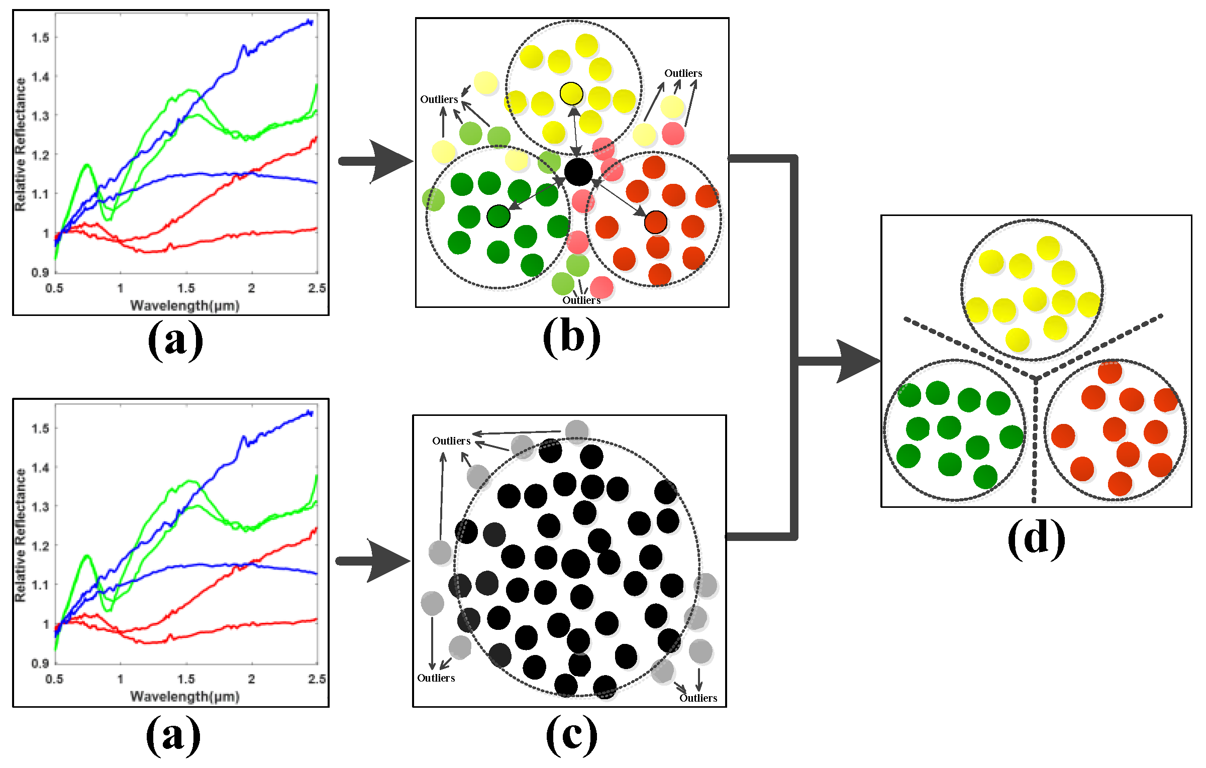
Figure 3.
The spectral preprocessing for (1) Ceres with category ‘C’. (a) Original spectra; (b) smoothed spectra; (c) fitted spectra spanning the wavelength range from 0.45 to 2.45 μm.
Figure 3.
The spectral preprocessing for (1) Ceres with category ‘C’. (a) Original spectra; (b) smoothed spectra; (c) fitted spectra spanning the wavelength range from 0.45 to 2.45 μm.
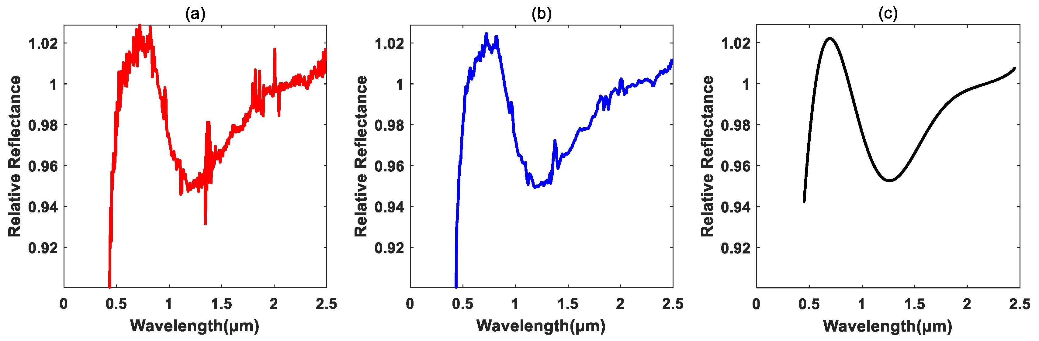
Figure 4.
The spectral preprocessing for (2957) Tatsuo with category ‘K’. (a) Original spectra; (b) smoothed spectra; (c) fitted spectra spanning the wavelength range from 0.45 to 2.45 μm.
Figure 4.
The spectral preprocessing for (2957) Tatsuo with category ‘K’. (a) Original spectra; (b) smoothed spectra; (c) fitted spectra spanning the wavelength range from 0.45 to 2.45 μm.
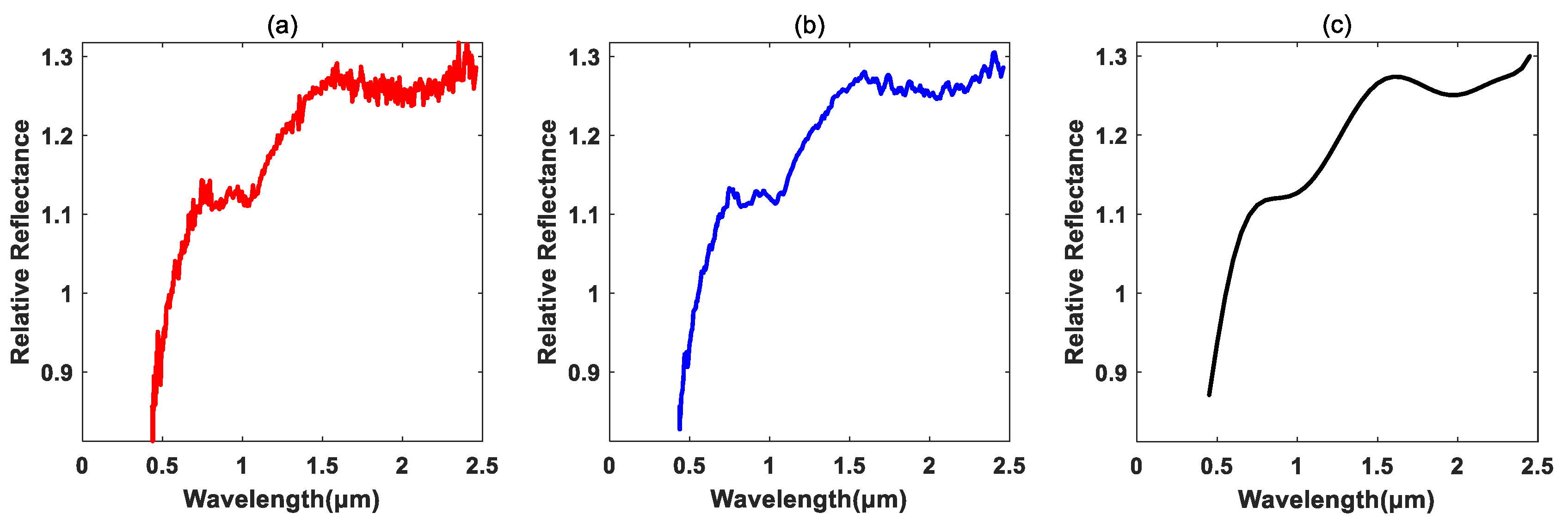
Figure 5.
The spectral preprocessing for (1807) Slovakia with category ‘S’. (a) Original spectra; (b) smoothed spectra; (c) fitted spectra spanning the wavelength range 0.45 to 2.45 μm.
Figure 5.
The spectral preprocessing for (1807) Slovakia with category ‘S’. (a) Original spectra; (b) smoothed spectra; (c) fitted spectra spanning the wavelength range 0.45 to 2.45 μm.

Figure 6.
Five-fold cross verification scheme for asteroid spectral data.

Figure 7.
The performance of different dimension reduction methods under different reduced dimensions using NN as the classifier.
Figure 7.
The performance of different dimension reduction methods under different reduced dimensions using NN as the classifier.

Figure 8.
The performance of different dimension reduction methods under different reduced dimensions using SVM as the classifier.
Figure 8.
The performance of different dimension reduction methods under different reduced dimensions using SVM as the classifier.
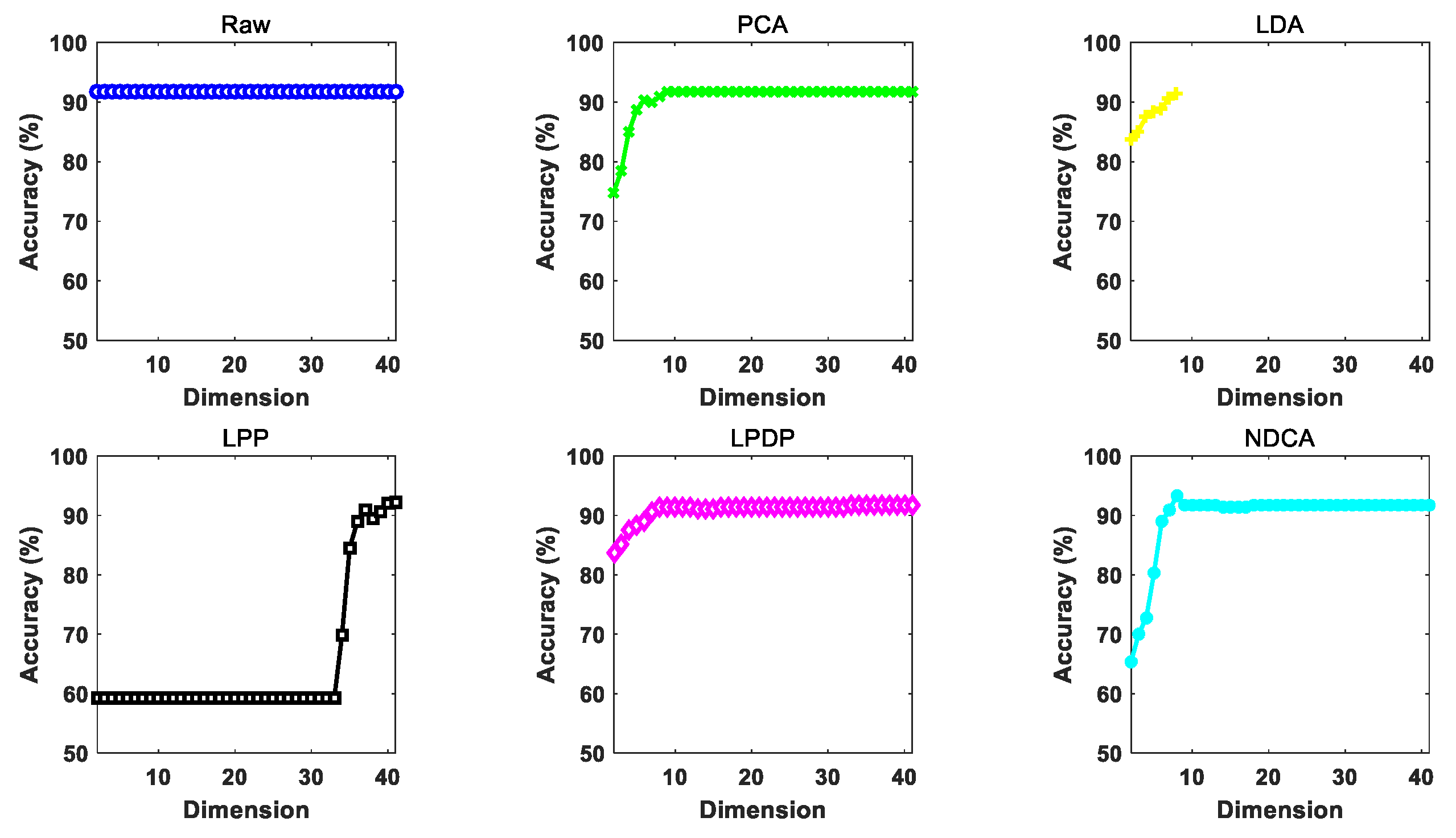
Figure 9.
The performance of different dimension reduction methods under different reduced dimensions using ELM as the classifier.
Figure 9.
The performance of different dimension reduction methods under different reduced dimensions using ELM as the classifier.

Figure 10.
Visualization for the scatter points of the first two components acquired by different methods. By comparison, the proposed NDCA model shows better within-class compactness and between-class separation characteristics.
Figure 10.
Visualization for the scatter points of the first two components acquired by different methods. By comparison, the proposed NDCA model shows better within-class compactness and between-class separation characteristics.

Figure 11.
NN plus NDCA performance under different combinations of parameters. (a) μ and γ (best: 90.60%; worst: 89.76%); (b) Rb and Rw (best: 92.81%; worst: 87.82%).
Figure 11.
NN plus NDCA performance under different combinations of parameters. (a) μ and γ (best: 90.60%; worst: 89.76%); (b) Rb and Rw (best: 92.81%; worst: 87.82%).

Figure 12.
SVM plus NDCA performance under different combinations of parameters. (a) μ and γ (best: 91.7009%; worst: 90.8676%); (b) Rb and Rw (best: 91.9787%; worst: 87.2679%).
Figure 12.
SVM plus NDCA performance under different combinations of parameters. (a) μ and γ (best: 91.7009%; worst: 90.8676%); (b) Rb and Rw (best: 91.9787%; worst: 87.2679%).

Figure 13.
ELM plus NDCA performance under different combinations of parameters. (a) μ and γ (best: 90.0894%; worst: 88.4365%); (b) Rb and Rw (best: 90.3676%; worst: 87.2660%).
Figure 13.
ELM plus NDCA performance under different combinations of parameters. (a) μ and γ (best: 90.0894%; worst: 88.4365%); (b) Rb and Rw (best: 90.3676%; worst: 87.2660%).

Figure 14.
Classification performance variations of NDCA plus ELM under different settings of L and α.
Figure 14.
Classification performance variations of NDCA plus ELM under different settings of L and α.

Table 1.
Description of the asteroid spectral datasets for 371 asteroids with 24 classes.
| Class | ‘A’ | ‘B’ | ‘C’ | ‘Cb’ | ‘Cg’ | ‘Cgh’ | ‘Ch’ | ‘D’ |
| # samples | 6 | 4 | 13 | 3 | 1 | 10 | 18 | 16 |
| Class | ‘K’ | ‘L’ | ‘O’ | ‘Q’ | ‘R’ | ‘S’ | ‘Sa’ | ‘Sq’ |
| # samples | 16 | 22 | 1 | 8 | 1 | 144 | 2 | 29 |
| Class | ‘Sr’ | ‘Sv’ | ‘T’ | ‘V’ | ‘X’ | ‘Xc’ | ‘Xe’ | ‘Xk’ |
| # samples | 22 | 2 | 4 | 17 | 4 | 3 | 7 | 18 |
Table 2.
Important notations used in this paper.
| Notation | Meaning | Notation | Meaning |
|---|---|---|---|
| P | Subspace projection matrix | T | Label matrix |
| X | High-dimensional dataset with dimension D | xi, xj | Data points with index i and j |
| Y | Lower-dimensional features of X with dimension d | N | Number of datapoints |
| C | Number of classes in X and Y | Ni, i = 1, 2 … C | Number of data points in i-th class |
| α | Balance parameter in ELM model | yi, yj | Lower-dimensional features for xi, xj |
Table 3.
Description of asteroid spectral datasets used in the experiments.
| Class | ‘A’ | ‘C’ | ‘D’ | ‘K’ | ‘L’ | ‘Q’ | ‘S’ | ‘V’ | ‘X’ | Total |
| # Samples | 6 | 45 | 16 | 16 | 22 | 8 | 199 | 17 | 32 | 361 |
Table 4.
Experimental data partition of 5-folds.
| Class | Fold 1 | Fold 2 | Fold 3 | Fold 4 | Fold 5 | Total |
|---|---|---|---|---|---|---|
| ‘A’ | 1 | 1 | 1 | 1 | 2 | 6 |
| ‘C’ | 9 | 9 | 9 | 9 | 9 | 45 |
| ‘D’ | 3 | 3 | 3 | 4 | 3 | 16 |
| ‘K’ | 4 | 3 | 3 | 3 | 3 | 16 |
| ‘L’ | 4 | 4 | 4 | 5 | 5 | 22 |
| ‘Q’ | 2 | 2 | 1 | 2 | 1 | 8 |
| ‘S’ | 40 | 40 | 40 | 40 | 39 | 199 |
| ‘V’ | 3 | 4 | 4 | 3 | 3 | 17 |
| ‘X’ | 6 | 6 | 7 | 6 | 7 | 32 |
| # samples | 72 | 72 | 72 | 73 | 72 | 361 |
Table 5.
Experiment settings with different fold partitions.
| Experiments | Training Dataset | Testing Dataset |
|---|---|---|
| Exp. 1 | fold 1, fold 2, fold 3 and fold 4 (289 samples in total) | fold 5 (72 samples in total) |
| Exp. 2 | fold 1, fold 2, fold 3 and fold 5 (288 samples in total) | fold 4 (73 samples in total) |
| Exp. 3 | fold 1, fold 2, fold 4 and fold 5 (289 samples in total) | fold 3 (72 samples in total) |
| Exp. 4 | fold 1, fold 3, fold 4 and fold 5 (289 samples in total) | fold 2 (72 samples in total) |
| Exp. 5 | fold 2, fold 3, fold 4 and fold 5 (289 samples in total) | fold 1 (72 samples in total) |
Table 6.
Classification accuracy (%) of different dimension reduction algorithms using NN as the classifier.
Table 6.
Classification accuracy (%) of different dimension reduction algorithms using NN as the classifier.
| Methods | Exp. 1 | Exp. 2 | Exp. 3 | Exp. 4 | Exp. 5 | Average |
|---|---|---|---|---|---|---|
| Raw | 94.4444 | 84.9315 | 87.5000 | 93.0556 | 86.1111 | 89.2085 |
| PCA | 94.4444 | 84.9315 | 87.5000 | 93.0556 | 86.1111 | 89.2085 |
| LDA | 95.8333 | 90.4110 | 88.8889 | 97.2222 | 88.8889 | 92.2489 |
| LPP | 90.2778 | 87.6712 | 90.2778 | 91.6667 | 88.8889 | 89.7565 |
| LPDP | 95.8333 | 90.4110 | 91.6667 | 97.2222 | 88.8889 | 92.8044 |
| NDCA | 97.2222 | 89.0411 | 93.0556 | 98.6111 | 93.0556 | 94.1971 |
Table 7.
Classification accuracy (%) of different dimension reduction algorithms using SVM as the classifier.
Table 7.
Classification accuracy (%) of different dimension reduction algorithms using SVM as the classifier.
| Methods | Exp. 1 | Exp. 2 | Exp. 3 | Exp. 4 | Exp. 5 | Average |
|---|---|---|---|---|---|---|
| Raw | 94.4444 | 86.3014 | 93.0556 | 93.0556 | 91.6667 | 91.7047 |
| PCA | 94.4444 | 89.0411 | 93.0556 | 93.0556 | 91.6667 | 92.2527 |
| LDA | 94.4444 | 90.4110 | 88.8889 | 94.4444 | 91.6667 | 91.9711 |
| LPP | 97.2222 | 86.3014 | 90.2778 | 95.8333 | 94.4444 | 92.8158 |
| LPDP | 94.4444 | 90.4110 | 93.0556 | 94.4444 | 91.6667 | 92.8044 |
| NDCA | 94.4444 | 90.4110 | 94.4444 | 95.8333 | 93.0556 | 93.6377 |
Table 8.
Classification accuracy (%) of different dimension reduction algorithms using ELM as the classifier.
Table 8.
Classification accuracy (%) of different dimension reduction algorithms using ELM as the classifier.
| Methods | Exp. 1 | Exp. 2 | Exp. 3 | Exp. 4 | Exp. 5 | Average |
|---|---|---|---|---|---|---|
| Raw | 94.8611 | 89.3151 | 92.0833 | 95.6944 | 91.5278 | 92.6963 |
| PCA | 95.0000 | 90.4110 | 92.0833 | 96.5278 | 92.3611 | 93.2766 |
| LDA | 95.4167 | 94.5205 | 91.8056 | 97.2222 | 93.4722 | 94.4874 |
| LPP | 95.8333 | 90.4110 | 93.0556 | 98.6111 | 94.4444 | 94.4711 |
| LPDP | 95.9722 | 94.5205 | 92.6389 | 97.2222 | 93.3333 | 94.7374 |
| NDCA | 97.7778 | 91.7808 | 93.4722 | 97.2222 | 95.6944 | 95.1895 |
Table 9.
Performance improvement between different pairs methods by using different classifiers.
| Classifiers | Comparison Pairs | ||||
|---|---|---|---|---|---|
| <Ours, Raw> | <Ours, PCA> | <Ours, LDA> | <Ours, LPP> | <Ours, LPDP> | |
| NN | ↑ 4.9886% | ↑ 4.9886% | ↑ 1.9482% | ↑ 4.4406% | ↑ 1.3927% |
| SVM | ↑ 1.9330% | ↑ 1.3850% | ↑ 1.6666% | ↑ 0.8219% | ↑ 0.8333% |
| ELM | ↑ 2.4932% | ↑ 1.9129% | ↑ 0.7021% | ↑ 0.7184% | ↑ 0.4521% |
Publisher’s Note: MDPI stays neutral with regard to jurisdictional claims in published maps and institutional affiliations. |
© 2021 by the authors. Licensee MDPI, Basel, Switzerland. This article is an open access article distributed under the terms and conditions of the Creative Commons Attribution (CC BY) license (https://creativecommons.org/licenses/by/4.0/).
Share and Cite
MDPI and ACS Style
Guo, T.; Lu, X.-P.; Zhang, Y.-X.; Yu, K. Neighboring Discriminant Component Analysis for Asteroid Spectrum Classification. Remote Sens. 2021, 13, 3306. https://0-doi-org.brum.beds.ac.uk/10.3390/rs13163306
AMA Style
Guo T, Lu X-P, Zhang Y-X, Yu K. Neighboring Discriminant Component Analysis for Asteroid Spectrum Classification. Remote Sensing. 2021; 13(16):3306. https://0-doi-org.brum.beds.ac.uk/10.3390/rs13163306
Chicago/Turabian StyleGuo, Tan, Xiao-Ping Lu, Yong-Xiong Zhang, and Keping Yu. 2021. "Neighboring Discriminant Component Analysis for Asteroid Spectrum Classification" Remote Sensing 13, no. 16: 3306. https://0-doi-org.brum.beds.ac.uk/10.3390/rs13163306
Note that from the first issue of 2016, this journal uses article numbers instead of page numbers. See further details here.