
SAR Imaging Distortions Induced by Topography: A Compact Analytical Formulation for Radiometric Calibration


National Research Council of Italy (CNR), Istituto per il Rilevamento Elettromagnetico dell’Ambiente (IREA), 80124 Napoli, Italy
Remote Sens. 2021, 13(16), 3318; https://0-doi-org.brum.beds.ac.uk/10.3390/rs13163318
Submission received: 30 June 2021
/
Revised: 15 August 2021
/
Accepted: 18 August 2021
/
Published: 22 August 2021
(This article belongs to the Special Issue Electromagnetic Modeling in Microwave Remote Sensing)
Abstract
:Modeling of synthetic aperture radar (SAR) imaging distortions induced by topography is addressed and a novel radiometric calibration method is proposed in this paper. An analytical formulation of the problem is primarily provided in purely geometrical terms, by adopting the theoretical notions of the differential geometry of surfaces. The novel and conceptually simple formulation relies on a cylindrical coordinate system, whose longitudinal axis corresponds to the sensor flight direction. A 3D representation of the terrain shape is then incorporated into the SAR imaging model by resorting to a suitable parametrization of the observed ground surface. Within this analytical framework, the area-stretching function quantitatively expresses in geometrical terms the inherent local radiometric distortions. This paper establishes its analytical expression in terms of the magnitude of the gradient of the look-angle function uniquely defined in the image domain, thus resulting in being mathematically concise and amenable to a straightforward implementation. The practical relevance of the formulation is also illustrated from a computational perspective, by elucidating its effective discrete implementation. In particular, an inverse cylindrical mapping approach is adopted, thus avoiding the drawback of pixel area fragmentation and integration required in forward-mapping-based approaches. The effectiveness of the proposed SAR radiometric calibration method is experimentally demonstrated by using COSMO-SkyMed SAR data acquired over a mountainous area in Italy.
1. Introduction
Synthetic aperture radar (SAR) is a side-looking imaging system whose recorded signal results from an electromagnetic wave scattering interaction process [1,2,3]. Indeed, the focused SAR image describes a complex-valued function defined in the (slant-range, azimuth) domain, and the associated power-detected received signal is proportional to the energy scattered by the observed extended target as a consequence of the radar illumination. The SAR radiometric calibration process is concerned with the conversion of the power-detected signal to scattering coefficients: the former are sensor-dependent measurements, the latter are physically meaningful quantities characterizing the scattering from imaged targets that are distributed in nature [3,4,5,6].
Radar scattering from distributed targets can be described by adopting different scattering coefficients, which must be inferred indirectly. In particular, the normalized radar cross section (NRCS) or scattering coefficient of a distributed target is defined as the average radar cross section (RCS) per unit illuminated area on the ground [3,4,5,6,7]. It is traditionally denoted by (sigma naught). A different scattering coefficient, usually denoted by , for characterizing scattering from distributed target is the RCS per unit effective surface area, which is defined in terms of the area perpendicular to the beam instead of the illuminated area on the ground [3,4,5,6]. Conversely, the radiometric quantity , which is commonly referred to as radar brightness, is defined as the average RCS per unit area in the SAR (slant-range, azimuth) image space [6,7,8,9]. Different from the above-mentioned coefficients, provides a sensor-dependent measurement. Moreover, quantitative electromagnetic modelling and interpretation canonically rely on scattering coefficients ( or ), which are physically meaningful descriptors of the inherent scattering phenomenon [10,11]. It is then clear that such indirectly obtained sensor-independent measurements, which are provided by a suitable SAR calibration process, are crucial for successively inferring meaningful information about physical parameters of the sensed distributed targets (inverse problem). Accordingly, SAR radiometric calibration is a fundamental operation that constitutes the premise of quantitative remote sensing applications.
As a matter of fact, the SAR imaging process involves different intrinsic distortive sources (e.g., range-spread loss, range-variant SAR compression gain, non-uniform antenna pattern illumination, etc.), which ultimately affect radiometric information conveyed by SAR data [6]. Different papers in recent decades have addressed the problem of SAR radiometric calibration by emphasizing different aspects [12,13,14,15,16,17,18,19,20,21,22,23].
In particular, in this paper, the emphasis is specifically placed on topography-induced radiometric distortions in SAR images, which are primarily caused by the imaging of the irregular ground. Such distortions cause SAR images to be radiometrically disturbed. Therefore, a priori knowledge about the 3D geometry of the observed scene and the SAR imaging configuration is required, in order to model and compensate for these unavoidable radiometric distortions.
It is worth noting that an SAR image provides a representation of the 3D object space in the 2D image space in which all the pixels have the same area, while the corresponding patches on the illuminated surface have different areas. It is clear that in order to reconstruct , which is defined in terms of the area of the ground surface [3,4,5,6], the effective area of the ground surface in the 3D space have to be evaluated on a pixel basis.
Remarkably, mountainous regions represent a rather extended portion of the Earth’s surface. Thus, compensation of the local radiometric distortions inherently introduced by the imaging process is of paramount importance, especially over high-relief landscapes. Various studies have addressed the radiometric effects of topography on SAR images, and different formulation and practical calibration procedures have been hitherto proposed. In particular, the formulation originally proposed in [17] introduces a correction method based on a geometric projection factor (which is also referred to as a cosine correction). Previous approaches [12,13,14,15] can be somehow regarded as approximations of the method in [17]. An important distinction concerns the domain in which the radiometric normalization is performed, and accordingly existing algorithms can be categorized in two main classes: algorithms operating in the map domain (e.g., in the geodetic coordinate system) (MD) and algorithms implementing compensation in the image domain (ID). For instance, the MD correction-based approach in [19] uses radar brightness integration of multiple image pixels, thus renouncing to the native SAR sensor resolution, even though energy preservation throughout the geocoding process is somehow addressed.
The generally used algorithm in [20] instead relies on an ID-based approach, in which a forward-mapping scheme is implicitly adopted. Moreover, it directly operates on vectorial functions defined in the 3D space, and it adopts a terrain description relying on a Delaunay triangulation. It should be noted that forward-mapping-based schemes typically suffer from the burden of pixel-area fragmentation and relevant integration [24]. In addition, adopting Delaunay triangulation might introduce abrupt changes in terrain slopes, as recognized in [25,26].
In this paper, an analytical formulation of the problem is primarily provided in purely geometrical terms, by adopting the theoretical notions of the differential geometry of surfaces [27]. The novel and conceptually simple formulation relies on a cylindrical coordinate system, whose longitudinal axis corresponds to the sensor flight direction. A 3D representation of the terrain shape is then incorporated into the SAR imaging model by resorting to a suitable parametrization of the observed ground surface. Within this analytical framework, the area-stretching function quantitatively expresses in geometrical terms the inherent local radiometric distortions. This paper establishes its analytical expression in terms of the magnitude of the gradient of the look-angle function uniquely defined in the image domain, which results in being mathematically concise and amenable to a straightforward implementation.
As a result, the established analytical formulation provides the mathematical background for the proposed SAR calibration method. The formulation, which is established in terms of continuous space functions, is then translated into its numerical counterpart that is also described and discussed in this paper. In particular, an inverse cylindrical mapping approach is adopted, thus avoiding the drawback of pixel-area fragmentation and integration [24]. The logical structure of the resulting calibration method reflects the advantages, in terms of conceptual and computational simplicity, of the compact analytical formulation, as discussed in the rest of the paper.
Finally, the implemented method has been applied to high-resolution X-band COSMO-SkyMed SAR data acquired over an Italian mountainous area, in order to demonstrate its practical effectiveness.
The paper is structured as follows. Section 2 presents the novel analytical formulation. Section 3 and Section 4 focus on the adopted inverse cylindrical mapping strategy and the numerical implementation of the proposed method, respectively. Results obtained by using real SAR data are shown in Section 5. Conclusions are finally drawn in Section 6.
2. Analytical Formulation
In this section, the emphasis is on the derivation of the novel analytical formulation, thus providing the theoretical concept behind the proposed calibration method.
2.1. Cylindrical Coordinate System
From a purely geometrical point of view, we assume that (at the scale of interest) the observed scene can be geometrically described by an (opaque) object bounded by an arbitrary smooth surface embedded in the 3D Euclidean space ().
The description of the topography of the remotely sensed scene is of primary importance for modelling topography-induced SAR radiometric distortions. As far as the representation of the scattering ground surface into the SAR image space is concerned, Cartesian coordinates have been commonly adopted [15,16,17,18,19,20]. However, dealing with a Cartesian representation might be inconvenient, because the subsequent analysis becomes unnecessarily complicated. Conversely, as will be clear in the rest of the paper, working with a coordinate system having the corresponding symmetry of the considered problem enables a simpler treatment of the problem itself. Specifically, the most natural frame for the representation of the observed scene shape, as viewed from the perspective of SAR sensor, is provided by a (curvilinear) cylindrical coordinate system.
Let be an orthonormal frame associated with a trajectory-centric Cartesian coordinate system, with the direction aligned with the SAR sensor flight direction and the direction oriented toward nadir point, as schematically illustrated in Figure 1. Cylindrical coordinates, denoted as , are defined with respect to the Cartesian frame , so that the longitudinal axis of the cylindrical frame corresponds to the path along which the sensor platform moves (see Figure 1). Accordingly, the position vector of an arbitrary target point of the illuminated scene can be expressed as , where the superscript 1 indicates that the representation is provided with respect to the frame . Provided that certain assumptions discussed in the following are satisfied, the cylindrical coordinates and may be interpreted as denoting slant-range (or across-track), look-angle (or elevation angle, or off-nadir angle), and azimuth (or along-track) coordinates, respectively.
The cylindrical basis vectors are tangent to the coordinate lines and form a right-handed orthonormal basis (see Figure 1), defined as follows:
It should be noted that cylindrical coordinates are not rectilinear, i.e., the coordinate lines are not straight lines, but they are orthogonal. Resorting to a sensor-oriented coordinate frame is particularly appropriate, since it enables the adoption of a convenient parametrization of the ground surface. This intuition is mathematically framed in the subsequent section.
2.2. Surface Parametric Representation
A suitable parametric representation of the ground surface illuminated by the SAR system is introduced in this section. A regular parameterization can be regarded as a one-to-one mapping from a parameter domain to the surface [27].
The sensor flight (azimuth) and slant-range directions define the SAR image space. Accordingly, and represent the slant-range and azimuth (continuous) coordinates in the SAR image space, respectively. A certain location in the SAR image space generally corresponds to a point of the 3D object space. Accordingly, the introduced cylindrical coordinate system suggests the adoption of the following parametric representation of the surface:
where is the parametric domain, and are the radar (parametric) range and azimuth coordinates in the image space, respectively. The sensor trajectory is described by vectored-value function , with the vector denoting the radar sensor position in the 3D space. Reasonably, it can be locally assumed as a linear path, hence its representation with respect to the orthonormal frame is given by .
As a result, the ground surface results to be naturally parametrized in terms of the function , which represents the look-angle function defined in the image space (Figure 2).
The adopted surface parameterization concerns with the mapping of the SAR image parametric domain onto the ground surface, since the adopted parametric coordinate space coincides with the SAR image space. Conversely, the inverse transformation pertains the mapping of the ground surface onto the 2D image space.
It should be noted that it has been assumed, for the sake of convenience, that the mapping defined by the Equation (2) constitutes a one-to-one correspondence at each of its regular point [27]. This assumption is however consistent with a domain that does not include layover and shadow regions. Since rigorous radiometric compensation cannot be achievable in such regions, we can conveniently exclude them from our analysis, without a loss of generality. The possible singular behavior of the transformation is further discussed in Section 2.7. As clarified in the next Section, the parametrization defined by the Equation (2) enables a convenient evaluation of the SAR radiometric distortions induced by the topographic reliefs.
2.3. Metric Properties
In this Section, the mapping associated with the vector-valued function is investigated, and the relevant fundamental quantities of interest are analytically derived.
The background to the following analytical investigation is provided by the differential geometry of surfaces; its theoretical foundations can be found, for instance, in [27].
The Jacobian matrix of the transformation assumes the following expression:
The first metric tensor of the surface is defined as , where T denotes the transpose operator [27]. By using (3), it assumes the form:
The tensor contains all the information necessary for calculating metric properties of the surface. For our purpose, the quantity of interest is the area of the ground surface embedded in the 3D object space, i.e., the domain in which the physical scattering phenomenon occurs as a consequence of the SAR illumination. By adopting the surface parametrization (2), the area of the ground surface can be formally defined as
In surface characterization [27], the area of the surface can be expressed as follows
where represents the determinant operator; and denote the vector cross product and the Euclidean norm, respectively. By substituting (4) in (6), the following expression is obtained:
where the differential quantity in (7) is referred to as the element of the surface area. It is expressed in terms of the magnitude of the gradient of the look-angle function, , which can be written as
where the vector
is referred to as the gradient of the look angle function at position in the image space, where the 2D operator is given in terms of Cartesian coordinates in the image space. For the sake of a lighter notation, in the following the functional dependence on the image space position of the look-angle function, of its partial derivatives, and of its gradient will be suppressed and understood.
Finally, it is instructive to highlight the distinction between the canonical nabla operator in 3D space, , and the operator acting in the 2D image space. For such a purpose, it is straightforward to verify that the following identity holds:
where the expression of in cylindrical coordinates is the following:
The presented formulation concerns the calculation of the area of the surface in the 3D object space that corresponds to a prescribed region in the SAR image -space. According to (7), the problem of measuring the area of the ground surface, accordingly, is reduced to a planar area measurement problem, by using the surface parametrization (2). The established functional form (7), therefore, takes an expression uniquely described in terms of the first-order partial derivatives of the look-angle function defined in the image space. One of the main results is this surprising simplification of the problem, since (7) takes a compact form. The compactness originates from the capability of the adopted cylindrical parametrization (2) in encoding the essential information contained in the scene topography (as seen by the sensor) into a form convenient for characterizing local radiometric distortions in SAR imaging.
As a result, the formulation, which is particularly appropriate to the SAR side-looking acquisition geometry, captures the nature of the problem in an expression that can be efficiently computed in the image domain (as discussed in Section 4).
2.4. Geometric Interpretation
The geometric interpretation of the established mathematical expression of the ground surface area (7) is now in order. It is worth emphasizing that the metric determinant quantity in (7), which pertains to the local transformation between the SAR image space and the ground surface in the observed 3D object space, can be geometrically interpreted in terms of the area-stretching function, , defined as:
Notice that describes a dimensionless quantity, which is also inherently a positive quantity. Conversely, the factor (with ) describes the local compression (foreshortening) of the elementary surface area in comparison with the corresponding elementary area in the SAR image space (Figure 2).
In particular, let be a rectangular subdomain, with area , representing an arbitrary pixel in the SAR -image space, where i and j are the corresponding (discrete) pixel coordinates, respectively. The associated ground surface in the 3D object space is described by . According to (7), the area of the illuminated patch on the ground can be written in the form:
where the expression on the right-hand side denotes integration of the area-stretching function over the area of the elemental domain (e.g., a pixel) in the image space (see Figure 2). The computation of (13) is discussed in detail in Section 4.
The portion of ground surface , as seen from the SAR imaging system, results in being foreshortened, because its apparent (or projected) area is equal to its real area multiplied by the factor . At the same time, this causes radiometric distortions in SAR images, since the apparent brightness of a ground surface depends on its actual ground surface area [3,4,5,6]. As a result, the SAR apparent “brightness” has to be equalized, in order to reconstruct a meaningful radiometric quantity (e.g., the backscattering coefficient). As evidenced by (12), the appropriate descriptors of the local foreshortening effect arising in SAR imaging of a scene with irregular topography are provided, rather than the terrain slopes, by the slopes of the geo-morphometric process evaluated in the image domain. Indeed, rather than the intrinsic geometric properties of topography, the descriptors based on the look-angle function conveniently capture the geometrical properties of the topography seen by the SAR sensor point of view. This is to say that the 3D scene topography information relevant to the SAR side-looking acquisition configuration is embedded in the look-angle function. This fact is interesting and suggests that a certain economy in the representation of the topography–induced radiometric distortions can be effectively achieved by working directly in the domain of the SAR image.
2.5. Local Incidence Angle
The outward-pointing normal vector of the surface, , is by definition the normal to the local tangent plane. For a surface in the 3D space described by the parametrization (2), according to the general notations introduced in the paper, can be written in the form:
The corresponding unit normal vector is , where
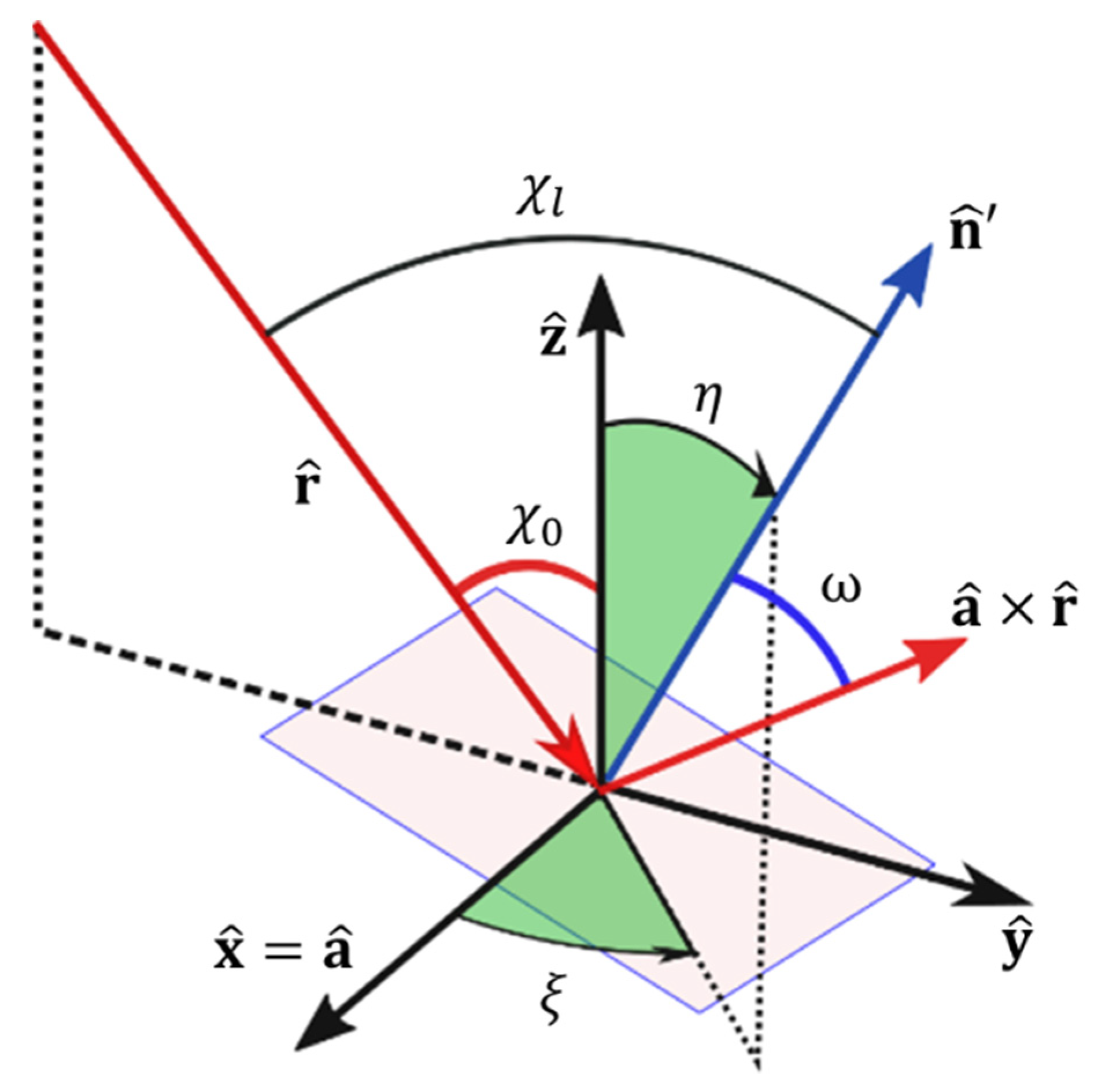
It should be noted that, according to the adopted surface orientation, is directed downward. Accordingly, the normal unit vector pointing toward the sensor direction is given as (see Figure 3). The local incidence angle is the angle defined by the incident radar beam and the normal to the intercepting surface (see Figure 3). According to the notation adopted in this paper, is the angle between (which represents the incoming radiation direction) and; thus obtaining .
We are now in position to establish an expression of the local incidence angle function defined in the image domain. Its functional form, by using (14) and (15), is directly obtained in terms of the partial derivatives of the look-angle function as follows:
Two limiting cases are worth of note. In the first case, approaches as vanishes, or else as . This condition arises at grazing angles or in stationary points. In the second case, a specular point occurs when vanishes, which in turn takes place as .
2.6. Analytical Consistency
It is instructive to compare the formulation proposed in this paper with the classical approach introduced in [17]. It can be easily demonstrated (see Appendix A for details) that the proposed formulation is consistent with the formalism in [17].
Nonetheless, the proposed formulation has interesting advantages, with respect to the commonly adopted cosine correction [17,22] that deserve some comments.
First, the mathematical description of the model in [17], which is given in terms of the so-called projection angle ω, incorporates several spatially variant functions (i.e., the local incidence angle of a horizontal ground , slope and aspect of the surface) jointly defining the local orientation of the ground surface with respect to the sensor (see Appendix A for details). Accordingly, it involves quantities that are natively defined in map geometry, thus making radiometric compensation in the image domain not straightforward. On the contrary, the proposed formulation essentially entails only the magnitude of the gradient of the look-angle function, which fully captures structural geometrical information about the scene topography relevant to the SAR acquisition configuration directly in the image domain, thus providing a compact expression that is also amenable to easy implementation (see Section 4).
Second, the notion of area-stretching function (or its reciprocal referred to as area-contraction function) might be more insightful with respect to the less intuitive geometrical descriptions relying on the projection angle ω (also referred to as projected local incidence angle or projection cosine approach [22]).
2.7. Singular Behavior
The observed ground surface has geometrically been characterized in terms of a parametrically defined surface, through the mapping from a parametric (2D) image space to the 3D object space. It has been assumed that constitutes a one-to-one transformation (see Section 2.2), by suitably excluding layover and shadow regions. Such an assumption deserves however further considerations.
It is rather intuitive to understand that the inverse mapping , which concerns the mapping from the 3D object space to a 2D image (parametric) domain, might indeed not be neither regular nor one-to-one in certain regions. From a mathematical perspective, this is to say that in correspondence to such regions the mapping is not a regular parametrization, although it can locally be considered one-to-one [27]. Accordingly, over certain spatial regions the mapping can exhibit a local folding. A possible folding that might occur is indeed associated with a spatial region affected by the well-known local layover phenomenon [28]. It is worth noting that the backscattering coefficient reconstruction cannot be rigorously and uniquely attained over layover regions (where only suboptimal radiometric corrections can be achieved) and it is meaningless over shadow regions (where no useful information is present).
Therefore, the considered parametrization reduces to the case of “foldover-free” parametrization by excluding layover and shadow regions. As a result, the one-to-one mapping assumption poses no practical limitations. Subsequently, the analytical expression (13) is generally applicable except over the layover and shadow regions. These regions might however be easily identified and excluded by the calibration procedure [28]. Nonetheless, a rigorous investigation of the radiometric response of layover regions deserves to be framed within an appropriate mathematical perspective (i.e., theory of singularities of smooth mappings and catastrophe theory) [29], thus it goes beyond the scope of this paper. In certain literature, the terms homeomorphism and homomorphism are subject of confusion [20], but they are indeed two distinct mathematical concepts.
3. Discrete Mapping
This section specifically concerns the discrete implementation of the continuous spatial mapping underlying the proposed analytical formulation. First, the problem is introduced in general (Section 3.1), and then the adopted discrete scheme is presented (Section 3.2).
3.1. Mapping in Digital Image Processing
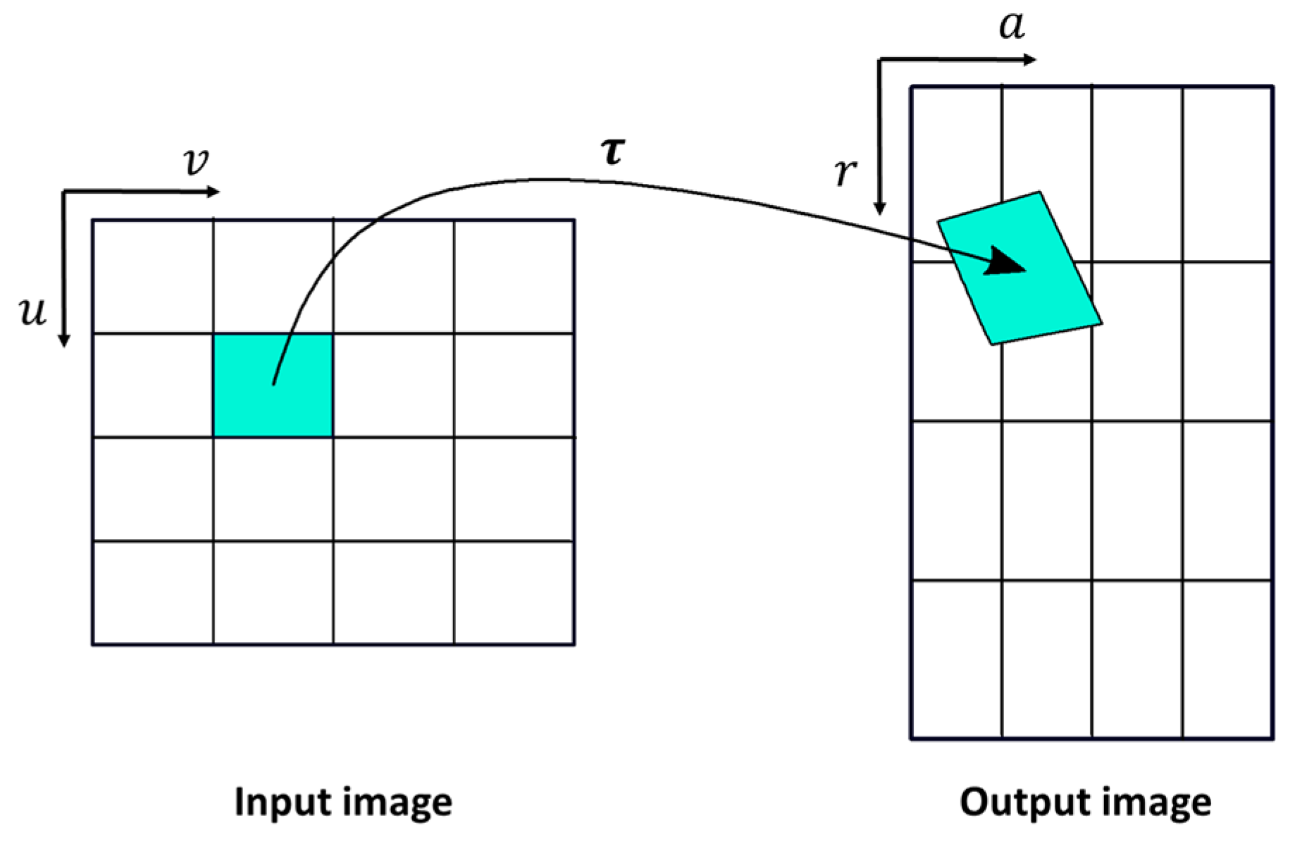
The mathematical formulation presented in Section 2 considers point-to-point mappings (spatial transformations) in the continuous domain. Conversely, as a discrete mapping is concerned, implementing a spatial transformation as point-to-point mapping might however be not appropriate [24], since pixels concern finite elements defined on a (discrete) integer lattice (Figure 4). In particular, here the focus is on the 2D to 2D spatial transformation , which is expressed as
It establishes a geometrical correspondence between a location in the (input) image, where and are the map coordinates [30], and a corresponding location in the SAR (output) image, where and are the range and azimuth coordinates (Figure 4). Therefore, is referred to as the forward mapping, whereas defines the inverse mapping.
As a matter of fact, the complications arising from the discretization of the transformation (17) have been widely investigated in the field of digital image processing, and discrete transformation implementation has been conducted according to suitable schemes, which can essentially be categorized into two main classes: forward and inverse mapping. A comprehensive treatment can be found in (Chapter 10 [24]).
Specifically, the forward mapping consists of copying the value of each pixel of the input image onto the output image at positions determined by the mapping function . As a matter of fact, the (uniformly spaced) samples of the input image generally result in being mapped in non-uniformly spaced locations (irregular sampling) in the output image domain. A four-corner (or three-corner) mapping paradigm is typically adopted. It considers input pixels as square patches that may be transformed into arbitrary quadrilaterals in the output image (Figure 4). The problem is that each pixel in the input image represents a finite (non-zero) area, and actually, the mapping projects a certain pixel of the input image onto the corresponding patch (which has a different area) in output space, as schematically shown in Figure 4. It should be noted that point-to-point mappings might generally give rise to two types of problems: holes and overlaps, because a transformed pixel of the input image straddles several pixels of the output image or is embedded in one pixel of the output image [24].
In particular, the fragments of the pixels of the input image contributing to each output pixel have to be determined, thus taking the fraction of the area of the input image pixel that covers the considered output image pixel as the weighting factor. Accordingly, this method requires an accumulator array and costly intersections (for deriving the weights and relevant scaling), to properly integrate the contributions of the input image pixels to each pixel of the output image [24].
In this regard, it is interesting to note that a forward (three-corner) mapping scheme has been adopted in the SAR calibration algorithm proposed in [20].
Another possibility, which is commonly adopted in digital image processing, is to resort to an inverse mapping scheme [24]. However, this convenient scheme requires that the explicit expression of the inverse transformation be available.
Here, the interest is specifically in the evaluation of the surface area on the ground corresponding to a prescribed pixel in the SAR (output) image space. It is assumed that the elevation of the topography is the information available on the (input) map-image domain, and that the associated ground area of each pixel of the input image is known. It is clear that (see Figure 4) the adoption of a canonical forward mapping scheme, for the estimation of the ground surface area corresponding to a certain pixel of the output image, inevitably has to deal with the burden of pixel-area fragmentation handling. Nonetheless, it is possible to circumvent the mentioned limitations by using a different strategy, which is introduced below.
3.2. Inverse Cylindrical Mapping
In this section, the adopted discrete mapping scheme, referred to as inverse cylindrical mapping, for the estimation of the ground surface area corresponding to an arbitrary pixel in the SAR image space, is presented. The proposed scheme permits us to avoid the drawbacks of forward-mapping schemes, without demanding the inverse transformation explicitly. This can be achieved by indirectly operating on the look-angle function, thus without requiring the direct transformation of the area information between different (input and output) domains, as discussed below.
Let us assume that the look-angle function is provided at regularly spaced locations in the (input) map image space.
First, input-image pixels are mapped in the (output) SAR image domain, as schematically illustrated in Figure 4; so, the forward mapping transforms a regular grid of locations in the input image domain in irregularly distributed locations in the output image domain. Therefore, the uniformly spaced samples of the look-angle function in the (input) map image are mapped in the (output) SAR image domain, thus resulting in an irregular distribution of samples.
Second, an interpolation stage (re-gridding) is considered, in order to reconstruct the values of the look-angle function at uniformly spaced locations in the SAR (output) image domain. Subsequently, the ground area corresponding to a prescribed image pixel can be directly computed in the (output) image space, according to (13).
In this way, the computed pixel-area associated with the (output) SAR image is finally mapped back to the corresponding ground surface area in the input image domain. Therefore, the inverse transformation is established indirectly, without explicitly demanding the inverse mapping . As a result, passing through the look-angle function computation, the pixel-area fragmentation and subsequent integration is indeed completely avoided. This constitutes an important advantage of the proposed scheme, as it does handle the transformation of the pixel-area indirectly. The advantages of the cylindrical inverse mapping will be further clarified in the next section.
4. Discrete Implementation
The analytical formulation developed in Section 2 describing the problem in terms of continuous-space functions is now translated into its discrete counterpart, which can be computed numerically. Accordingly, the main aspects of the numerical implementation are discussed in the following, highlighting also the approximations inherent in the solution of the associated discrete problem.
4.1. Range-Doppler Backward Georeferencing
The first processing step concerns the evaluation of the look-angle function starting from the orbital information and the digital elevation model (DEM) of the terrain.
DEM data is typically defined in terms of topographic elevation and geodetic latitude–longitude map coordinates, and it is provided in a raster-format. Terrain information can be then represented in a 3D Earth-centered Earth fixed (ECEF) geocentric Cartesian reference system, in order to be compared with satellite orbit information [2].
Afterward, the well-known Range–Doppler (RD) geolocation method converts Cartesian coordinates of a point target on the ground into image () coordinates [31,32]. Accordingly, each ground position can then be mapped to a corresponding location in the (range, azimuth) coordinate image space, by using satellite ephemerids data. The procedure of the RD method is also referred to as backward georeferencing. It relies on the solution of a nonlinear system including Doppler and slant-range equations, which can be solved iteratively with a very fast convergence [2,31,32].
By using simple geometric relationships, the look-angle can be evaluated for each position on the ground, as well. As a result, in addition to the computed image coordinates, information on the corresponding look-angle is also attained for each ground point. Accordingly, a discrete version of the look-angle map is obtained at irregularly spaced data points in the -space. As a result, the computed look-angle function, which incorporates topographic elevation information in a convenient form, inherits somehow the intrinsic discrete representation of the employed digital elevation model, as discussed in the next section.
4.2. Look-Angle Function Regridding
The application of the RD backward geolocation procedure yields the evaluation of the look-angle function at locations that are irregularly positioned in the -image space (Section 4.1). Consequently, a suitable interpolation scheme must be used to reconstruct the discrete version of the look-angle function on a prescribed regular grid in the same image domain, with and denoting the (discrete) range and azimuth coordinates, respectively. Having at our disposal the look-angle function resampled on a regular grid enables straightforward computation of the relevant gradient in the image domain (Section 4.3).
Numerous methods for spatial interpolation have been developed in various disciplines, and selecting an appropriate spatial interpolation method for a specific function is not an easy task. In particular, data reconstruction is commonly performed by using canonical nearest neighbor and linear interpolation; however, modelling topographic data with a piecewise constant or piecewise linear functions leads to an inaccurate description in the case of interest. On the contrary, high-quality global interpolation methods (e.g., thin plate spline), in which every interpolated point depends explicitly on every data point, might be computationally impracticable, especially as very large datasets are concerned. Nonetheless, some local interpolation methods (e.g., inverse distance weighting, local Kriging) achieve computational efficiency at the expense of somewhat arbitrary restrictions on the form of the fitted surface.
As a matter of fact, the appropriate representation of the look-angle function shape is an important prerequisite for accurate ground area measurement; accordingly, the adoption of a shape preserving interpolation scheme is crucial within the proposed framework. Therefore, the well-known Akima’s method of bivariate interpolation and smooth surface fitting for irregularly distributed data points, which employs a local fifth-degree polynomial, is specifically adopted in this investigation. Akima’s interpolation method was originally introduced in [33], and it has several desirable properties. Specifically, the resulting interpolated surface is continuous and smooth and does not exhibit erroneous undulations. The method does not smooth the data, i.e., the resulting surface passes through all the given points if the method is applied to smooth surface fitting. It is also important to remark that this method has no problems concerning computational stability or convergence. Finally, note that such a re-gridding algorithm can be a time-consuming process, but it is much faster than global methods. Since the reconstruction of a single scalar function (i.e., the look-angle function) is needed in the adopted framework, the associated computational cost still appears reasonable.
4.3. Image Domain Processing
It is assumed that the look-angle function is given on a prescribed regular grid in the image space. Let be a rectangle representing an arbitrary pixel in the SAR image space, where i and j are the (discrete) coordinates of the pixel along range and azimuth directions, respectively. The corresponding illuminated surface in the 3D object space is , and the model (13) mathematically takes into account the area of the ground surface area corresponding to a prescribed SAR pixel . The radiometric quantity of interest can then be obtained directly in the image domain, by compensating for the distortive factor on a pixel-by-pixel basis. Accordingly, the energy-preserving reconstruction of is obtained accordingly to the Equation:
where is the (observable) radar brightness (also referred to as beta-nought) associated with the pixel with discrete coordinates and [9]. It should be noted that the area associated with an SAR image pixel, , is a constant. Equation (18) takes into account predictable local radiometric distortions (which are therefore correctable) in the SAR imaging system induced by the ground topography; thus, the inherent compensation ensures correct normalization and energy conservation.
Computation of the ground surface area is in order. According to (13), the problem of measuring the area of the ground surface in the 3D object space has been reduced to the evaluation of the area of a parametric surface defined in the image space, which is a purely 2D problem. Indeed, the integral in (13) might be computed in different ways [34]. Notice that area is additive; thus, the area of a set can be measured by partitioning the set into subsets and adding the areas of these subsets. Specifically, we can consider a regular partition (in sub-rectangles) of in the -space, thus leading to a partition of the 3D surface in which each partition element is denoted by . Summing up over all rectangles, the approximate area of the surface can be written as
where in represents the area-stretching function (12) evaluated (on a regular grid) at the discrete coordinates, and , in the image space. The expression (19) provides the discrete counterpart of the continuous-space function in (13). In the limit (as △r, △a →0) where the partition becomes finer and finer, the limit of the Riemann sum from (19) tends toward (13) [34]. In practice, the partition might also reduce to a single element as long as the variability of inside the domain of integration is negligible.
In particular, the function appearing in (19) is given in terms of the magnitude of the gradient of the scalar function defined in the image space (see (8), (12)), thus enabling a particularly convenient implementation. Therefore, its evaluation encompasses the computation of first-order partial derivatives of the look-angle function . The partial derivatives have to be estimated, through finite differences, from the discrete version (obtained on a regular grid) of the look-angle function . Numerical procedures for estimating the partial derivatives are, however, not unique.
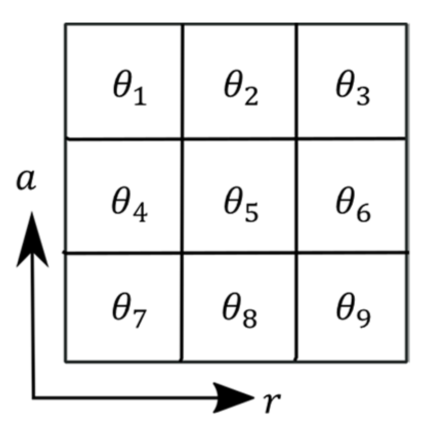
The most popular algorithms for computing first (and second) derivatives from gridded data operate on an N × N window centered at a prescribed point (a 3 × 3 grid kernel is shown in Figure 5), where the parameter N is an odd integer (see for instance [35,36]). Such a window provides accordingly a natural orthogonal parameterization that can be used to compute partial derivatives with respect to the parametric coordinates.
Specifically, we adopt the Evans–Young central finite-difference scheme, because it is the best for gradient (i.e., it has the lowest standard error and mean error), as demonstrated in [35]. The adopted scheme fits a second order polynomial to the 3 × 3 neighborhood filter, thus achieving a stable result in the presence of any error in the data [36]. As a result, first partial derivatives can be calculated according to a central difference representation [35,36], as follows (see Figure 5):
The estimation of the partial derivatives of look-angle function at each point of the regular mesh, therefore, can be performed easily by convolving the image data points with a set of local window operators (kernel), according to (20) and (21). Therefore, components of the gradient are obtained as follows
where ∗ denotes the convolution operation, and and are suitable 3 × 3 kernels. It is worth highlighting that, in principle, the proposed computational scheme naturally provides an adaptive mechanism for controlling the accuracy of the solution, for prescribed SAR image pixel dimensions and resolution of the digital elevation model. To clarify this point some brief considerations are in order.
Intuitively, the surface curvature is the rate at which the surface deviates from its tangent plane; a more formal description is provided in [27]. Accordingly, for a prescribed number of elements of the partition in (19), the accuracy of the computation depends on the curvature of the function .
Conversely, the accuracy of parametric-surface area estimation (19) can be preserved by controlling the number of elements of the partition in (19) (and subsequently the grid spacing and ) to accommodate the curvature of the considered surface. Therefore, the proposed formulation naturally allows different SAR sensors, and high resolution topographic information to be used for SAR calibration. Therefore, more sophisticated approaches could also be considered, but they are beyond the scope of this paper. For instance, finer meshes could be adopted in highly curved regions and coarser meshes in low curvature regions (e.g., they could also be considered quad-tree based or locally adaptive strategies [37]), in order to combine a good approximation with fast computation.
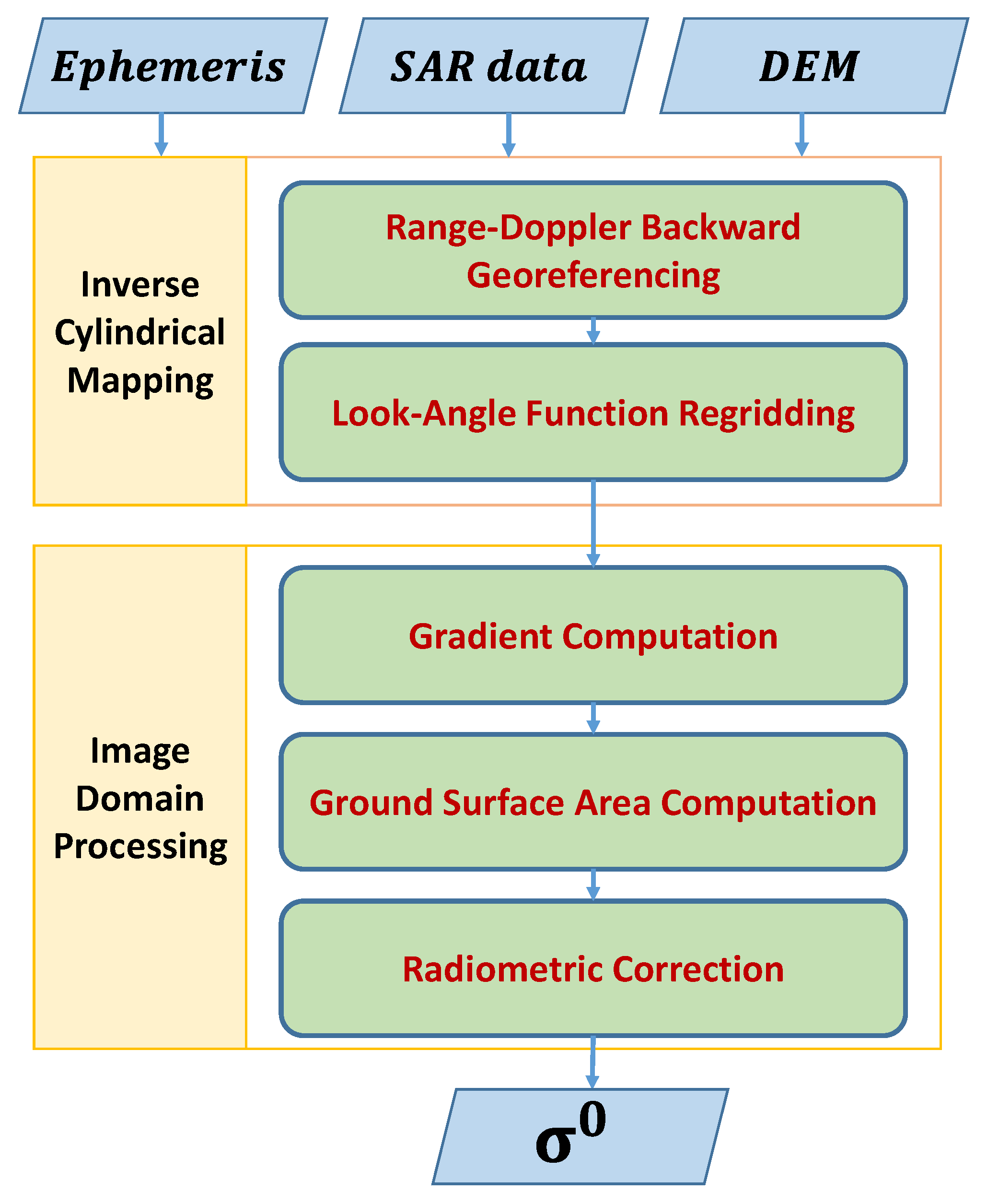
To conclude, the overall computation pattern is summarized by the synoptic representation depicted in Figure 6. First, the look angle function is obtained over an irregular grid in the image domain, according to the classical RD backward georeferencing procedure (Section 4.1), and then it is suitably resampled on a prescribed regular grid, as discussed in Section 4.2. Subsequently, gradient estimation is carried out in the SAR image domain according to (20) and (21). Next, for each pixel in the image domain, the formula (19) is evaluated for obtaining a corresponding estimation of the area of the illuminated surface in the 3D object space. Finally, the SAR image is radiometrically equalized, on a pixel-by-pixel basis, accordingly to (18).
5. Experimental Results
In this section, the proposed method is implemented and applied to real SAR data to demonstrate its practical effectiveness. As a case study, a site located in the province of L’Aquila (between the Gran Sasso and the Monti della Laga), Abruzzi, Italy, is considered, which is morphologically rather complex, including mountain, submontane and river valleys reliefs. The adopted methodology has been implemented by using a digital elevation model (DEM) of the terrain obtained via the NASA-JPL Shuttle Radar Topography Mission (SRTM) dataset. SRTM data used for this study is provided in WGS84 unprojected geographic latitude-longitude coordinates at a relatively fine resolution, with a 1-arc-second (approximately 30 m grid-cell size) pixel spacing, which permits us to derive the terrain descriptor values for the area under investigation.
Notice that the actual spatial resolution of SRTM 1-arc-second data has been estimated in the range from 50 to 80 m [38]. Note that shadow and layover areas have been modelled and identified accurately, according to the rigorous approach in [28]. An X-band COSMO-SkyMed (CSK) raw SAR data acquired in HH-polarization and strip map mode on 12 April 2009, over the area of interest, has been selected for our experiments. The SLC image has been obtained by properly focusing the SAR raw (Level 0) data [39]; the pixel size is 2.33 m × 1.33 m (azimuth × slant-range). Key parameters of the SAR data used in this study are summarized in Table 1. The coverage map of the SAR image is also reported in Table 1 in terms of geodetic latitude and longitude coordinates.
The entire SAR data has been processed; however, for the sake of convenience, in the following we focus our discussion on a 12,000 × 12,000 (pixels) portion of the image. The range direction is from left to right; the azimuth direction is from bottom to top.
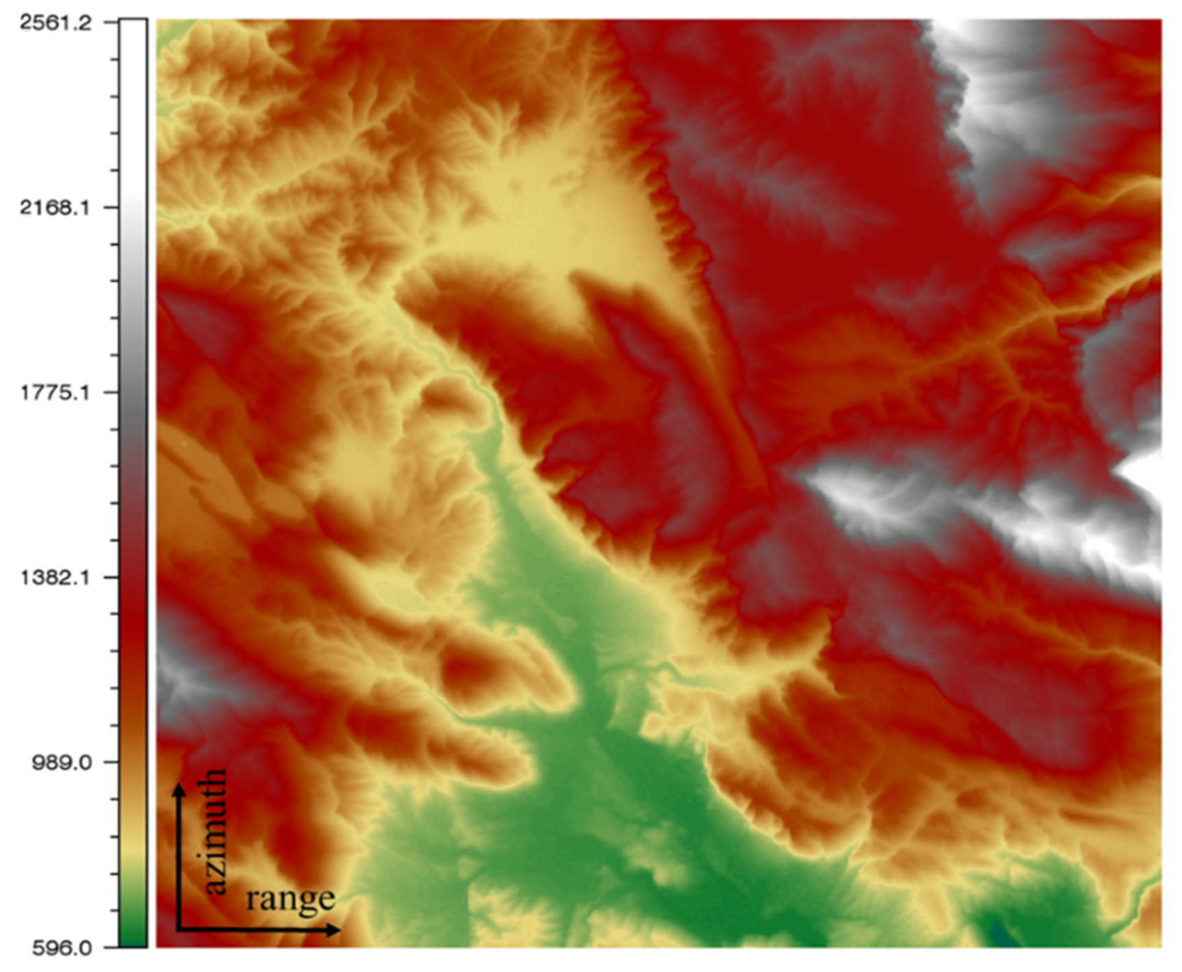
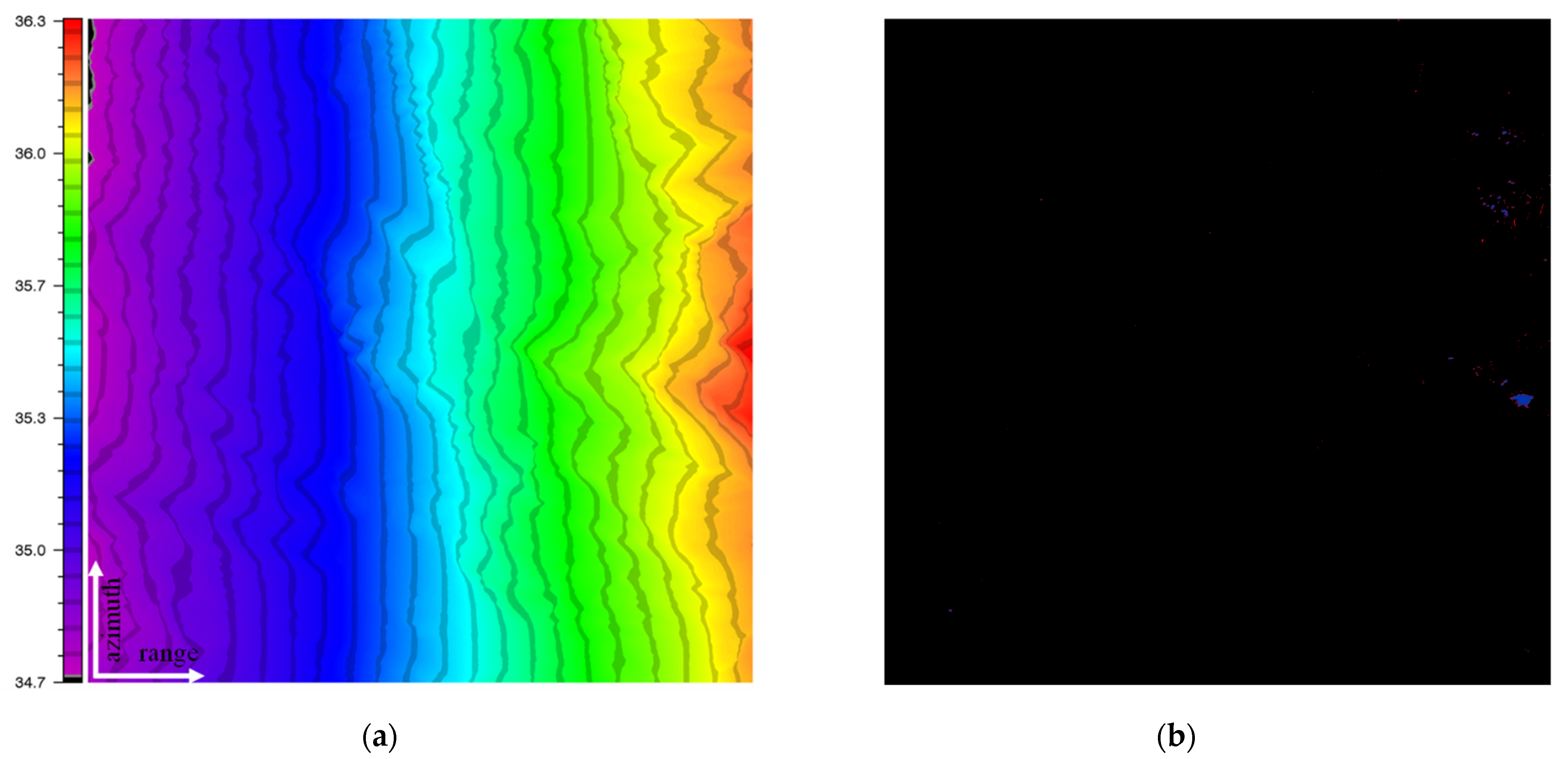
The altitude of the considered area ranges from 596 to 2561 m above sea level, and the mean altitude is 1128.95 m. The DEM elevation (in meters) representation in the image space is depicted in Figure 7 The look-angle function (LAF), , has been reconstructed on a regular grid in the image domain, by using satellite ephemeris and topographic SRTM data for the area under investigation, as discussed in Section 4. Figure 8a shows the computed LAF (in degree) according to a color-coded representation in the image space. It is worth noting that there are some localized regions of the considered image where the radiometric information is not reliable. They are associated with shadow- and layover-affected areas, including no useful or partial information, respectively.
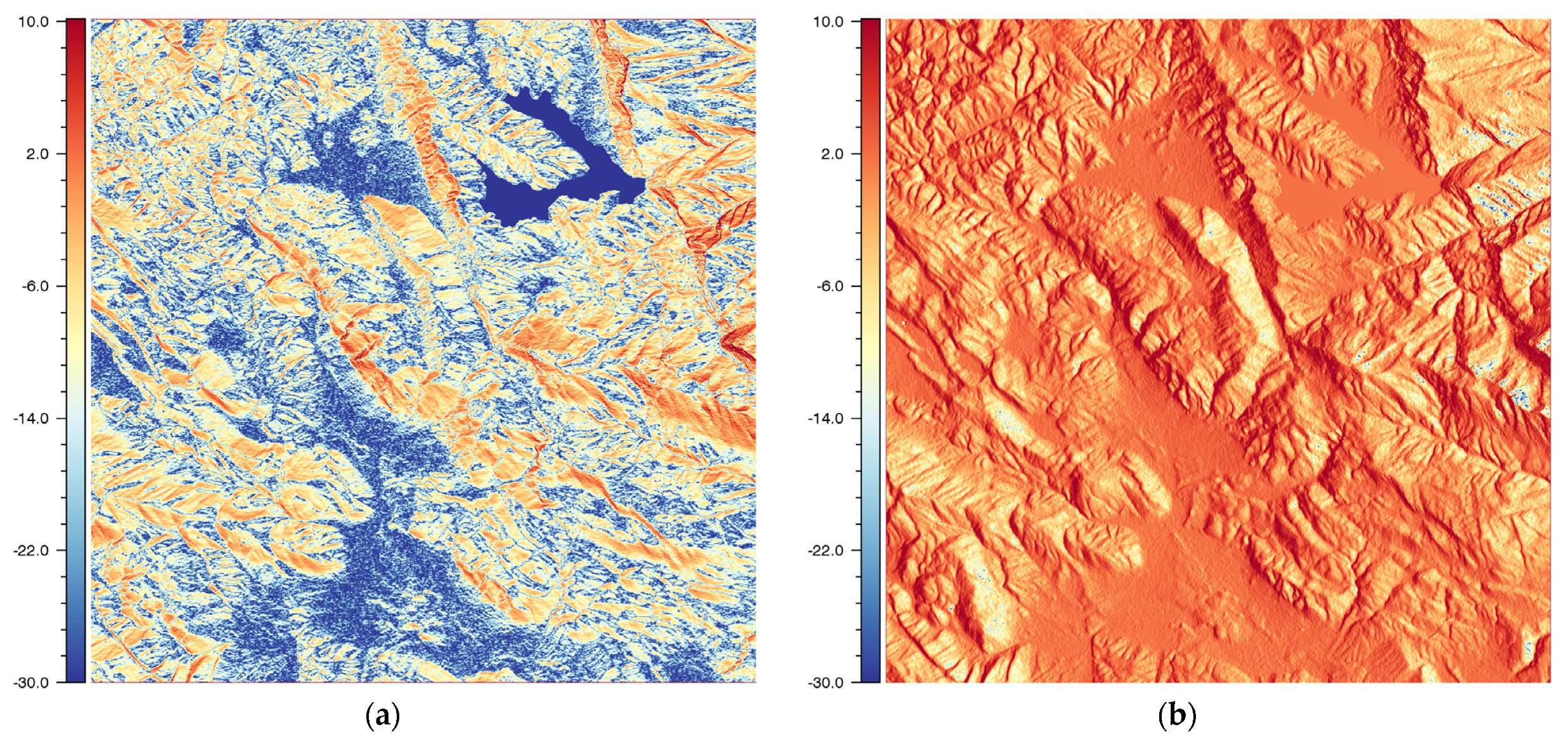
Accordingly, layover and shadowing regions have preliminarily been identified by using orbital and topographic information, according to the rigorous approach in [28]. Figure 8b depicts the classified layover (in red) and shadow (in blue) regions. In the case under investigation, these regions represent about 0.2% of the total number of image pixels. Moreover, the magnitude of the (range-weighted) partial derivatives of the LAF along the azimuth () and range () directions have been computed; they are depicted in Figure 9a,b, respectively. Remarkably, the investigated region includes the Campotosto artificial lake, which is a reservoir located at an elevation of 1313 m and comprised of an area of about 14 km2. The characteristic “V” shaped pattern, which is clearly recognizable in Figure 9a, is indeed associated with the surface lake.
As expected, over the lake surface the azimuthal variation of the LAF function is negligible (note that the dark-blue pattern is associated with the lake area, according to the color-coded representation in Figure 9a). Consistently, over the same lake area, a nonzero range variation of the LAF is attained (see Figure 9b).
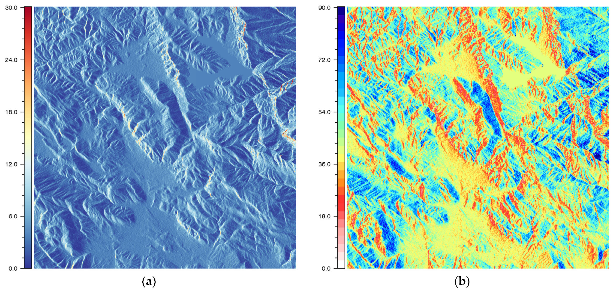
By combining the results of Figure 9a,b, the simulated radiometric distortions associated with the local ground surface area can be reconstructed directly in the image domain, according to (13); it is depicted (in dB) in Figure 10a by using a different color-coded image representation.
According to (16), the local incidence angle (LIA), , can be evaluated in the image domain directly in terms of the partial derivatives of the LAF; it is illustrated in Figure 10b.
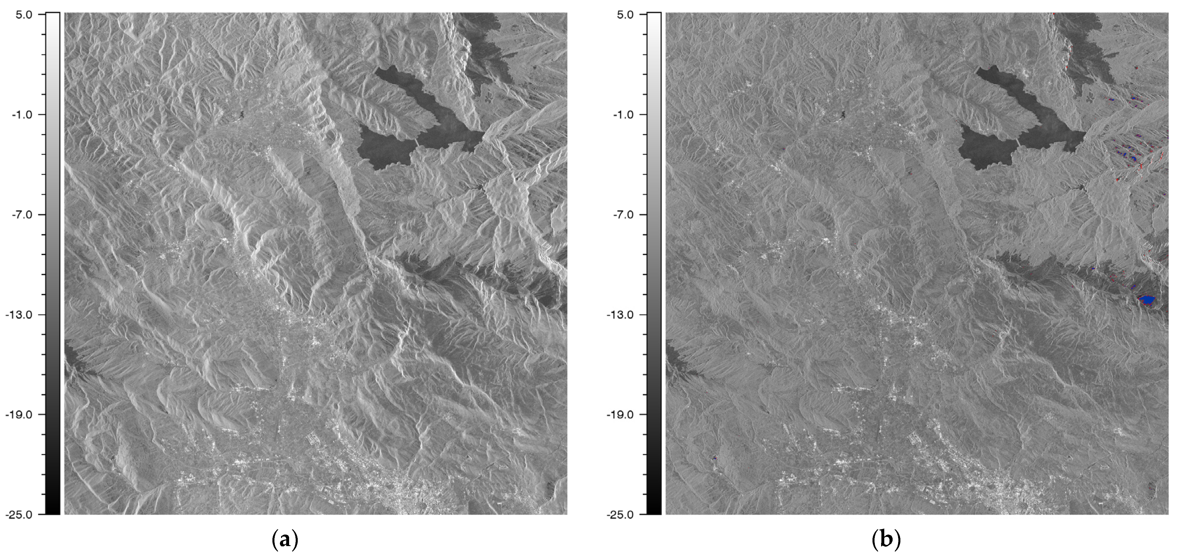
The image of the uncompensated backscattering coefficient (dB) (or pseudo backscattering coefficient) depicted in Figure 11a has been directly obtained from the SLC image by applying the absolute calibration constant only, thus not including any compensation of topography-induced radiometric distortions. As is evident from Figure 11a, the uncompensated is strongly affected by local variations, with a modulation over the imaged scene that is largely ascribed to the inherent local radiometric distortions induced by reliefs. By visual inspection of Figure 10a and Figure 11a, it is evident the matching between the pattern in the uncompensated backscattering coefficient (Figure 11a) and the simulated distortion image associated with the effective ground surface area (Figure 10a). Therefore, by using the simulated radiometric distortions depicted in Figure 10a, the local radiometric distortions (see Figure 11a) have ultimately been rectified, thus reconstructing the (true) backscattering coefficient image shown in Figure 11b. Moreover, in order to masked out regions in which radiometric information is not reliable, a mask representing the identified layover (red) and shadow (blue) is shown superimposed in Figure 11b. As can be seen from Figure 11b, the strong distortions appearing in the uncompensated image have largely been removed, while the dependence on the ground cover class is preserved.
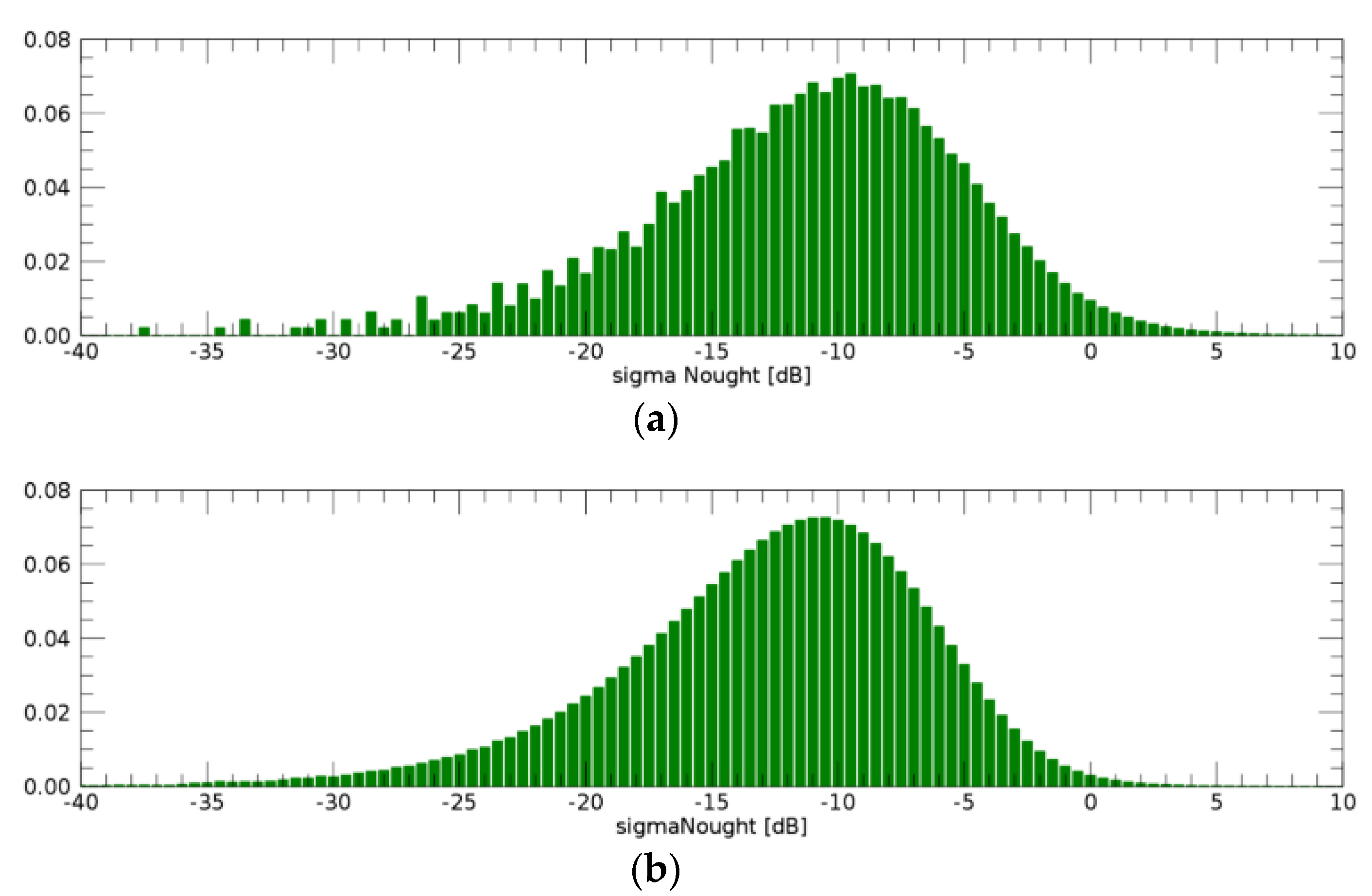
In addition, the distributions of the scattering coefficient, obtained without and with the compensation of topography-induced radiometric distortions, are depicted in Figure 12a,b, respectively.
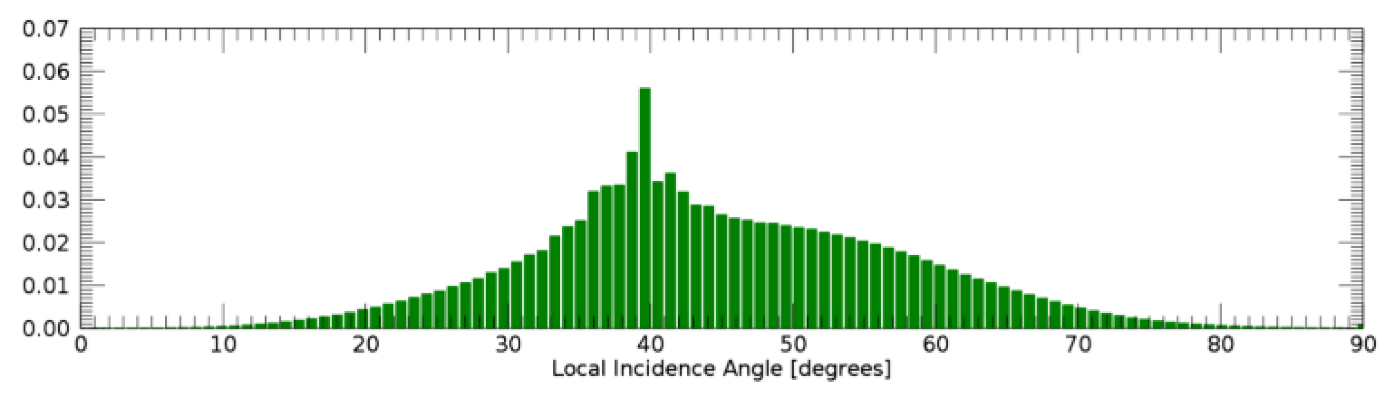
The distribution function of the LIA is displayed in the range (0, 90°) in Figure 13.
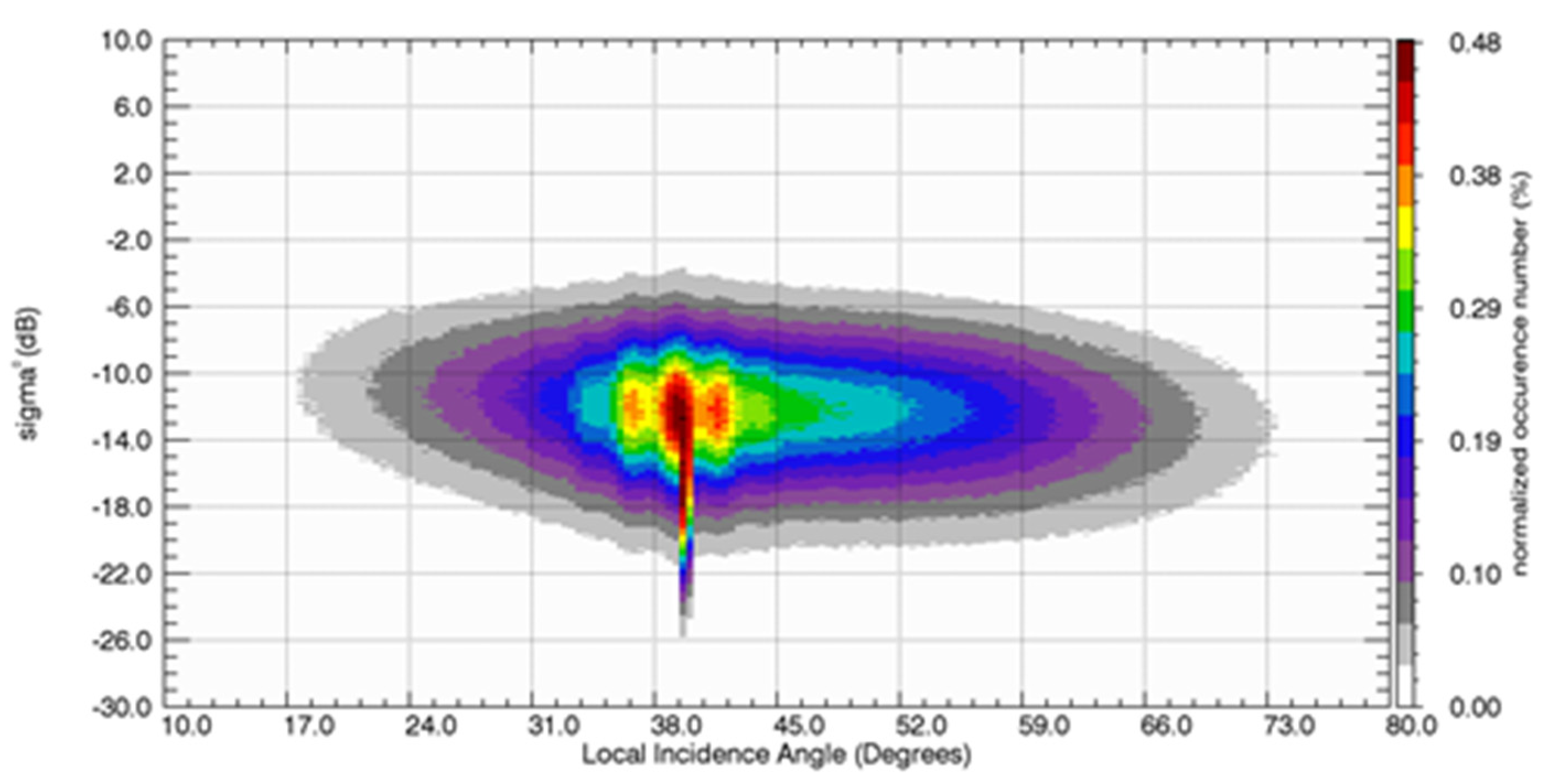
In order to further show the effect of the applied radiometric compensation quantitatively, the scatterplots in Figure 14a and Figure 15 represent the backscattering coefficient (in dB) versus the local incidence angle (in degree), respectively before and after the compensation of the topography-induced distortions.
In particular, the color bars represent different classes assigned to different colors; they are characterized by the number of occurrence (in %) normalized to the total number of image samples. The joint analysis of the scatterplots in Figure 14 and Figure 15 also provide an insight in the effect of the compensation on the backscattering signature. Figure 14 shows a sharp dependence upon the local incidence angle. By direct inspection, it is evident that the overall dependency on the local incident angle, occurring in the distribution depicted in Figure 14, results in being significantly reduced after the application of the radiometric compensation (see Figure 15).
Therefore, the proposed method successes in predicting/correcting the imaging distortions induced by surface topography that locally affect SAR images. Nonetheless, it should be noted that the normalized backscattering coefficient obtained by applying the pixel-by-pixel radiometric compensation is dependent on the LIA, as the local scattering properties of the distributed target also depends on the LIA [3,4,5]. As can be recognized from Figure 11b, such a dependency is however preserved.
More precisely, the backscattering coefficient at a certain point of the observed scene might be expressed in terms of the functional form , where is the LIA and is the vector representing the (geometric and dielectric) local parameters of the surface or layered structure [40,41] (e.g., interfacial roughness, dielectric permittivity, vegetation cover, etc.). The -dependence formally underlines the fact that might be locally sensitive to the electromagnetic and geometric properties of the ground cover class. Accordingly, distinct land cover types might exhibit different angular signatures [3,4]. In order to fully explore the specific angular dependence of the backscattering coefficient, the use of scattering models for distributed-target and electromagnetic theory might be appropriate [3,4,5,41].
Finally, it is important to highlight that the SAR radiometric calibration process, as done for obtaining the results presented in this paper, should also include the compensation of the additional radiometric distortions (e.g., range-spread loss, antenna pattern illumination) that are systematically introduced by the SAR system [6]. However, their comprehensive discussion is beyond the scope of this paper.
6. Conclusions
This paper presents an innovative formulation for modelling topography-induced radiometric distortions affecting SAR images, thus resulting in a straightforward SAR calibration method.
The effectiveness of the simple computational structure of the calibration method primary resides in the underlying compact analytical formulation of the problem. The adopted formulation specifically encompasses a suitable 3D geometric description based on a trajectory-centric cylindrical coordinate system, a convenient parametrization of the surface on the ground, and an inverse cylindrical (discrete) mapping approach. Accordingly, it has the following salient advantages:
- (1)
- The adopted formalism is rigorously derived by using the fundamental concepts of differential geometry of surfaces [27].
- (2)
- The expression of the local radiometric distortion has been established in analytical form, in terms of the magnitude of the gradient of a scalar function defined in the SAR image space. Such a function is indeed the look-angle function, which analytically captures in a convenient form the information on the topographic reliefs as seen by the sensor.
- (3)
- The proposed formalism turns out compact and expressive; further, accordingly, the inherent look-angle based encoding scheme can be valuable because of its ease of implementation. As a matter of fact, the novel formulation reduces the problem to a 2D domain calculation, with relevant computation carried out on a regular grid in the image domain, thus requiring only scalar functions handling, with important implications in terms of computational efficiency.
- (4)
- The proposed formulation maintains also the local consistency with the classical approach in [17]. Nonetheless, the area-stretching concept might be more insightful with respect to the projection angle notion.
- (5)
- The proposed method completely circumvents the drawback of the pixel-area fragmentation issue, because it follows an approach based on a cylindrical inverse mapping. Conversely, the existing forward-mapping-based approaches [24] entail the burden of pixel-area fragmentation and relevant integration [20].
In this paper, the practical effectiveness of the calibration method has also been demonstrated by using high-resolution SAR data acquired over a mountain site located in Italy. It should be also stressed that, once the radiometric compensation has been applied in the image domain, the calibrated SAR image can also be orthorectified, according to [2].
Finally, it is important to highlight that the proposed method is amenable to further interesting developments. In particular, the introduced formalism might be extended to describe the polarization orientation angle shifts induced by topography [42]. In addition, the evaluation of the effective area of the surface, for the evaluation of the gamma-naught backscattering coefficient, can also be conducted within the same formal framework. However, such an extension deserves further analytical derivations, and it will be matter of a forthcoming paper. Further investigations will be also devoted to the application of the proposed method to data acquired by other SAR sensors (Sentinel-1, SAOCOM, ALOS-2 PALSAR-2, etc.) and to high-resolution DEMs.
Funding
This research received no external funding.
Conflicts of Interest
The author declares no conflict of interest.
Appendix A
This Appendix A demonstrates the analytical consistency of the proposed formulation. For such a purpose, the formalism in [17] is briefly introduced (see Figure 3); it is referred to as a ground Cartesian frame , as illustrated by the scheme in Figure 3. The local orientation of the ground surface is accordingly described in terms of the spherical angles and , which correspond to slope and aspect of the surface relative to vertical () and azimuth () directions, respectively (see Figure 3). The projection angle ω (cosine correction), according to the model in [17], is defined by the formula:
where = denotes the incidence angle of a horizontal surface patch on the ground. Therefore, the expression (A1) relates the cosine correction to three different angles describing the local orientation of the ground surface with respect to the sensor. It is worth noting that in the special case of no local slope component (), the expression (A1) reduces to . By expressing the surface normal unit vector in terms of spherical angles (, the expression (A1) can be rewritten in the form:
Accordingly, the projection angle ω represents the angle between and the image-plane normal vector . Notice that the surface orientation induced by the parametrization, is opposed to that toward the sensor (i.e., ).
On the other hand, by using (12), (14), (15), it is easy to verify that
We are now in position to compare the novel expression (12) with the formalism (A1), (A2) of [17]. By direct inspection of (A2) and (A3) and noting that , it can be directly verified that
It follows that (A3) is fully consistent with (A1) and (A2), provided that an infinitesimal surface patch is considered. It should be noted that the meaning of the sign in (A2) is related to orientation, but here we are concerned only with areas, so we take absolute values of (A2). As a result, the proposed formulation is locally consistent with the formalism in [17].
References
- Curlander, J.C.; McDonough, R. Synthetic Aperture Radar, Systems & Signal. Processing; Wiley: New York, NY, USA, 1991. [Google Scholar]
- Schreier, G. Geometrical properties of SAR images. In SAR Geocoding: Data and Systems; Wichmann: Karlsruhe, Germany, 1993; pp. 103–134. [Google Scholar]
- Ulaby, F.T.; Moore, R.K.; Fung, A.K. Microwave Remote Sensing: Active and Passive. Volume 2-Radar Remote Sensing and Surface Scattering and Emission Theory; Addison-Wesley: Boston, MA, USA, 1982. [Google Scholar]
- Ulaby, F.T.; Moore, R.K.; Fung, A.K. Microwave Remote Sensing: Active and Passive—Volume Scattering and Emission Theory, Advanced Systems and Applications; Artech House, Inc.: Dedham, MA, USA, 1986; Volume III. [Google Scholar]
- Tsang, L.; Kong, J.A.; Shin, R.T. Theory of Microwave Remote Sensing; Wiley: New York, NY, USA, 1985. [Google Scholar]
- Freeman, A. SAR calibration: An overview. IEEE Trans. Geosci. Remote Sens. 1992, 30, 1107–1121. [Google Scholar] [CrossRef]
- Knott, E.F.; Shaeffer, J.F.; Tuley, M.T. Radar Cross Section; SciTech Publishing: Raleigh, NC, USA, 2004. [Google Scholar]
- Peake, W. Interaction of electromagnetic waves with some natural surfaces. IRE Trans. Antennas Propag. 1959, 7, 324–329. [Google Scholar] [CrossRef] [Green Version]
- Raney, R.K.; Freeman, T.; Hawkins, R.W.; Bamler, R. A plea for radar brightness. In Proceedings of the IGARSS’94-1994 IEEE International Geoscience and Remote Sensing Symposium, Pasadena, CA, USA, 8–12 August 1994. [Google Scholar]
- Imperatore, P.; Iodice, A.; Riccio, D. Electromagnetic Wave Scattering From Layered Structures with an Arbitrary Number of Rough Interfaces. IEEE Trans. Geosci. Remote. Sens. 2009, 47, 1056–1072. [Google Scholar] [CrossRef]
- Imperatore, P.; Azar, R.; Calo, F.; Stroppiana, D.; Brivio, P.A.; Lanari, R.; Pepe, A. Effect of the Vegetation Fire on Backscattering: An Investigation Based on Sentinel-1 Observations. IEEE J. Sel. Top. Appl. Earth Obs. Remote. Sens. 2017, 10, 4478–4492. [Google Scholar] [CrossRef]
- Freeman, A.; Curlander, J.C. Radiometric correction and calibration of SAR images. Photogramm. Eng Remote. Sens. 1989, 55, 1295–1301. [Google Scholar]
- van Zyl, J.J. The effect of topography on radar scattering from vegetated areas. IEEE Trans. Geosci. Remote. Sens. 1993, 31, 153–160. [Google Scholar] [CrossRef]
- Holecz, F.; Meier, E.; Piesbergen, J.; Nuesch, D.; Moreira, J. Rigorous derivation of backscattering coefficient. IEEE Geosci. Remote. Sens. Soc. Newslett 1994, 6–14. [Google Scholar]
- van Zyl, J.J.; Chapman, B.D.; Dubois, P.; Shi, J. The effect of topography on SAR calibration. IEEE Trans. Geosci. Remote. Sens. 1993, 31, 1036–1043. [Google Scholar] [CrossRef]
- Sarabandi, K. Calibration of a polarimetric synthetic aperture radar using a known distributed target. IEEE Trans. Geosci. Remote. Sens. 1994, 32, 575–582. [Google Scholar] [CrossRef]
- Ulander, L.M.H. Radiometric slope correction of synthetic-aperture radar images. IEEE Trans. Geosci. Remote. Sens. 1996, 34, 1115–1122. [Google Scholar] [CrossRef]
- Leclerc, G.; Beaulieu, N.; Bonn, F. A simple method to account for topography in the radiometric correction of radar imagery. Int. J. Remote. Sens. 2001, 22, 3553–3570. [Google Scholar] [CrossRef] [Green Version]
- Löw, A.; Mauser, W. Generation of geometrically and radiometrically terrain corrected SAR image products. Remote. Sens. Environ. 2007, 106, 337–349. [Google Scholar] [CrossRef]
- Small, D. Flattening gamma: Radiometric terrain correction for SAR imagery. IEEE Trans. Geosci. Remote. Sens. 2011, 49, 3081–3093. [Google Scholar] [CrossRef]
- Shimada, M. Model-based polarimetric SAR calibration method using forest and surface-scattering targets. IEEE Trans. Geosci. Remote. Sens. 2011, 49, 1712–1733. [Google Scholar] [CrossRef]
- Frey, O.; Santoro, M.; Werner, C.L.; Wegmuller, U. DEM-based SAR pixel-area estimation for enhanced geocoding refinement and topographic normalization. IEEE Geosci. Remote. Sens. Lett. 2013, 10, 48–52. [Google Scholar] [CrossRef]
- Imperatore, P.; Lanari, R.; Pepe, A. GICAL: Geo-Morphometric Inverse Cylindrical Method for Radiometric Calibration of SAR Images. In Proceedings of the IGARSS 2018-IEEE International Geoscience and Remote Sensing Symposium, Valencia, Spain, 23–27 July 2018; pp. 7840–7843. [Google Scholar]
- Jähne, B. Digital Image Processing; Springer: Berlin/Heidelberg, Germany, 2002. [Google Scholar]
- Biniaz, A.; Dastghaybifard, G. Slope fidelity in terrains with higher order Delaunay triangulations. In Proceedings of the WSCG, Plzen, Czech Republic, 4–7 February 2008. [Google Scholar]
- Biniaz, A.; Dastghaibyfard, G. Drainage Reality in Terrains with Higher-Order Delaunay Triangulations. Advances in 3D Geoinformation Systems; Springer: Berlin/Heidelberg, Germany, 2008. [Google Scholar]
- Carmo, P.M.d. Differential Geometry of Curves and Surfaces; Prentice-Hall: Englewood Cliffs, NJ, USA, 1976. [Google Scholar]
- Kropatsch, W.G.; Strobl, D. The generation of SAR layover and shadow maps from digital elevation models. IEEE Trans. Geosci. Remote. Sens. 1990, 28, 98–107. [Google Scholar] [CrossRef]
- Arnol’d, V.I. Catastrophe Theory; Springer Science & Business Media: Berlin/Heidelberg, Germany, 2003. [Google Scholar]
- Iliffe, J. Datums and Map Projections for Remote Sensing, GIS, and Surveying; CRC Press: Boca Raton, Florida, USA, 2000. [Google Scholar]
- Curlander, J. Location of space borne SAR imagery. IEEE Trans. Geosci. Remote. Sens. 1982, GRS-20, 359–364. [Google Scholar] [CrossRef]
- Curlander, J.C. Utilization of spaceborne SAR data for mapping. IEEE Trans. Geosci. Remote. Sens. 1984, GE-22, 106–112. [Google Scholar] [CrossRef]
- Akima, H. A method of bivariate interpolation and smooth surface fitting for irregularly distributed data points. ACM Trans. Math. Softw. (TOMS) 1978, 4, 148–159. [Google Scholar] [CrossRef]
- Evans, G. Practical Numerical Integration; Wiley: New York, NY, USA, 1993. [Google Scholar]
- Hengl, T.; Reuter, H.I. (Eds.) Geomorphometry: Concepts, Software, Applications; Newnes: Oxford, UK, 2008; Volume 33. [Google Scholar]
- Hengl, T.; Evans, I.S. Mathematical and digital models of the land surface. Dev. Soil Sci. 2009, 33, 31–63. [Google Scholar]
- Frey, P.J.; George, P.-L. Mesh Generation: Application to Finite Elements, 2nd ed.; Wiley: New York, NY, USA, 2010. [Google Scholar]
- Pierce, L.; Kellndorf, J.; Walker, W.; Barros, O. Evaluation of the horizontal resolution of SRTM elevation data. Photogramm. Eng. Remote. Sens. 2006, 72, 1235–1244. [Google Scholar] [CrossRef]
- Imperatore, P.; Pepe, A.; Lanari, R. Spaceborne Synthetic Aperture Radar Data Focusing on Multicore-Based Architectures. IEEE Trans. Geosci. Remote. Sens. 2016, 54, 4712–4731. [Google Scholar] [CrossRef]
- Imperatore, P.; Iodice, A.; Pastorino, M.; Pinel, N. Modelling scattering of electromagnetic waves in layered media: An up-to-date perspective. Int. J. Antennas Propag. 2017. [Google Scholar] [CrossRef] [Green Version]
- Ishimaru, A. Wave Propagation and Scattering in Random Media; Academic Press: New York, NY, USA, 1993. [Google Scholar]
- Imperatore, P.; Pepe, A.; Lanari, R. Polarimetric SAR Distortions Induced by Topography: An Analytical Formulation for Compensation in the Imaging Domain. In Proceedings of the IGARSS 2018-IEEE International Geoscience and Remote Sensing Symposium, Valencia, Spain, 23–27 July 2018; pp. 6353–6356. [Google Scholar]
Figure 1.
Cylindrical coordinate system.

Figure 2.
SAR imaging process: geometric scheme.

Figure 3.
3D geometrical scheme of a ground surface patch: is the surface unit normal, is local incidence angle, is the projection angle, and are the vertical and azimuth directions, respectively.
Figure 3.
3D geometrical scheme of a ground surface patch: is the surface unit normal, is local incidence angle, is the projection angle, and are the vertical and azimuth directions, respectively.

Figure 4.
Schematic illustration of the discrete mapping for spatial transformation ), with and .

Figure 5.
3 × 3 Grid kernel.

Figure 6.
Processing Scheme.

Figure 7.
Elevation (m) of the DEM: representation in the image space. The range direction is from left to right; the azimuth direction is from bottom to top.
Figure 7.
Elevation (m) of the DEM: representation in the image space. The range direction is from left to right; the azimuth direction is from bottom to top.

Figure 8.
The range direction is from left to right; the azimuth direction is from bottom to top: (a) Look Angle Function (LAF) (degree):; (b) a mask identifying (red) layover and (blue) shadow areas.
Figure 8.
The range direction is from left to right; the azimuth direction is from bottom to top: (a) Look Angle Function (LAF) (degree):; (b) a mask identifying (red) layover and (blue) shadow areas.

Figure 9.
Magnitude of the (range-weighted) partial derivative of look-angle function along: (a) the azimuth direction (dB), ; (b) the range direction (dB), .
Figure 9.
Magnitude of the (range-weighted) partial derivative of look-angle function along: (a) the azimuth direction (dB), ; (b) the range direction (dB), .

Figure 10.
(a) Simulated radiometric-distortion image (dB) associated with the ground surface area; (b) local incidence angle (LIA) (degree): .
Figure 10.
(a) Simulated radiometric-distortion image (dB) associated with the ground surface area; (b) local incidence angle (LIA) (degree): .

Figure 11.
(a) (dB) image obtained from SAR data without compensation of topography-induced radiometric distortions; (b) (dB) image obtained from SAR data including the compensation of topography-induced radiometric distortions. A mask identifying (red) layover and (blue) shadow areas is superimposed.

Figure 12.
Distribution of the backscattering coefficient (dB): (a) obtained without compensation of topography-induced radiometric distortions; (b) obtained by including the compensation of topography-induced radiometric distortions.
Figure 12.
Distribution of the backscattering coefficient (dB): (a) obtained without compensation of topography-induced radiometric distortions; (b) obtained by including the compensation of topography-induced radiometric distortions.

Figure 13.
Distribution of the local incidence angle (LIA) [degree].

Figure 14.
Backscattering coefficient [dB] without the compensation of topography-induced distortions vs. local incidence angle [degree].
Figure 14.
Backscattering coefficient [dB] without the compensation of topography-induced distortions vs. local incidence angle [degree].

Figure 15.
Backscattering coefficient (dB) after the compensation of topography-induced distortions vs. local incidence angle (degree).
Figure 15.
Backscattering coefficient (dB) after the compensation of topography-induced distortions vs. local incidence angle (degree).


Table 1.
SAR Dataset Characteristics.
| SAR Sensor | CSK | |
|---|---|---|
| Acquisition Date | 12 April 2009 | |
| Observation Direction | Right looking | |
| Polarization | HH | |
| Orbit | 7260 | |
| Orbit Direction | Ascending | |
| Carrier Frequency (GHz) | 9.60 | |
| Off-nadir Angle (degree) | 35.90 | |
| Sampling Frequency (MHz) | 112.50 | |
| Chirp Bandwidth (MHz) | 42.00 | |
| PRF (Hz) | 3104.31 | |
| Range Pixel Spacing (m) | 1.33 | |
| Azimuth Pixel Spacing (m) | 2.34 | |
| First near | (latitude (deg), longitude (deg)) | (42.145, 13.202) |
| First far | (42.215, 13.755) | |
| Last near | (42.562, 13.103) | |
| Last far | (42.632, 13.660) | |
Publisher’s Note: MDPI stays neutral with regard to jurisdictional claims in published maps and institutional affiliations. |
© 2021 by the author. Licensee MDPI, Basel, Switzerland. This article is an open access article distributed under the terms and conditions of the Creative Commons Attribution (CC BY) license (https://creativecommons.org/licenses/by/4.0/).
Share and Cite
MDPI and ACS Style
Imperatore, P. SAR Imaging Distortions Induced by Topography: A Compact Analytical Formulation for Radiometric Calibration. Remote Sens. 2021, 13, 3318. https://0-doi-org.brum.beds.ac.uk/10.3390/rs13163318
AMA Style
Imperatore P. SAR Imaging Distortions Induced by Topography: A Compact Analytical Formulation for Radiometric Calibration. Remote Sensing. 2021; 13(16):3318. https://0-doi-org.brum.beds.ac.uk/10.3390/rs13163318
Chicago/Turabian StyleImperatore, Pasquale. 2021. "SAR Imaging Distortions Induced by Topography: A Compact Analytical Formulation for Radiometric Calibration" Remote Sensing 13, no. 16: 3318. https://0-doi-org.brum.beds.ac.uk/10.3390/rs13163318
Note that from the first issue of 2016, this journal uses article numbers instead of page numbers. See further details here.