Article

Cloud Detection Algorithm for Multi-Satellite Remote Sensing Imagery Based on a Spectral Library and 1D Convolutional Neural Network

1
School of Geoscience, China University of Petroleum, Qingdao 266580, China
2
College of Geodesy and Geomatics, Shandong University of Science and Technology, Qingdao 266590, China
3
State Key Laboratory of Resources and Environmental Information Systems, Institute of Geographic Sciences and Natural Resources Research, Chinese Academy of Sciences, Beijing 100101, China
4
College of Oceanography and Space Information, China University of Petroleum, Qingdao 266580, China
*
Author to whom correspondence should be addressed.
Remote Sens. 2021, 13(16), 3319; https://0-doi-org.brum.beds.ac.uk/10.3390/rs13163319
Submission received: 4 July 2021 / Revised: 12 August 2021 / Accepted: 18 August 2021 / Published: 22 August 2021

Abstract

:
Automatic cloud detection in remote sensing images is of great significance. Deep-learning-based methods can achieve cloud detection with high accuracy; however, network training heavily relies on a large number of labels. Manually labelling pixel-wise level cloud and non-cloud annotations for many remote sensing images is laborious and requires expert-level knowledge. Different types of satellite images cannot share a set of training data, due to the difference in spectral range and spatial resolution between them. Hence, labelled samples in each upcoming satellite image are required to train a new deep-learning-based model. In order to overcome such a limitation, a novel cloud detection algorithm based on a spectral library and convolutional neural network (CD-SLCNN) was proposed in this paper. In this method, the residual learning and one-dimensional CNN (Res-1D-CNN) was used to accurately capture the spectral information of the pixels based on the prior spectral library, effectively preventing errors due to the uncertainties in thin clouds, broken clouds, and clear-sky pixels during remote sensing interpretation. Benefiting from data simulation, the method is suitable for the cloud detection of different types of multispectral data. A total of 62 Landsat-8 Operational Land Imagers (OLI), 25 Moderate Resolution Imaging Spectroradiometers (MODIS), and 20 Sentinel-2 satellite images acquired at different times and over different types of underlying surfaces, such as a high vegetation coverage, urban area, bare soil, water, and mountains, were used for cloud detection validation and quantitative analysis, and the cloud detection results were compared with the results from the function of the mask, MODIS cloud mask, support vector machine, and random forest. The comparison revealed that the CD-SLCNN method achieved the best performance, with a higher overall accuracy (95.6%, 95.36%, 94.27%) and mean intersection over union (77.82%, 77.94%, 77.23%) on the Landsat-8 OLI, MODIS, and Sentinel-2 data, respectively. The CD-SLCNN algorithm produced consistent results with a more accurate cloud contour on thick, thin, and broken clouds over a diverse underlying surface, and had a stable performance regarding bright surfaces, such as buildings, ice, and snow.

1. Introduction

As clouds continuously cover approximately 66% of the earth’s surface, they are ubiquitous in satellite remote sensing images [1,2,3]. The presence of clouds greatly hinders the accuracy and reliability of the inversion of surface and atmospheric parameters in quantitative remote sensing, such as the monitoring of land use and land cover changes and the retrievals of the aerosol optical depth, surface temperature, and particulate matter [4,5,6]. Therefore, automatic and efficient cloud detection is of great significance for subsequent remote sensing image analysis.
Cloud detection studies have been previously conducted; cloud detection methods are primarily divided into two categories: physical rule-based detection methods and machine learning methods. Clouds are characterised by a high reflectivity in the visible and near-infrared bands and a low temperature in the thermal infrared bands [7]. Physical rule-based methods are used to identify clouds and clear-sky pixels based on the spectral differences or low temperature properties of the clouds and surface in different wavebands. The function of the mask (Fmask) algorithm, a representative cloud detection method, produces a cloud detection probability map for Landsat-8 images based on different threshold values of both cloud reflection characteristics and the brightness temperature [8,9]. The Moderate Resolution Imaging Spectroradiometer (MODIS) cloud mask algorithm also applies the threshold method in order to obtain MODIS cloud mask products [10,11]. The threshold method has been widely adopted in cloud detection; however, the selection of the band and threshold strongly depends on the analysis of spectral differences between the cloud layers and typical surface features. Due to the complex surface environment and the diversity of cloud geometries, it is typically difficult to fully consider the influencing factors in order to determine the optimal threshold [12]. In addition, the threshold-based method is sensitive to the changes in the atmospheric conditions and scene attributes and lacks versatility when transferred to other sensors [13]. Clouds dynamically change and the images of the same location obtained at different times notably differ. Therefore, using the differences between multi-temporal image pixels is important to detect clouds and clear-sky pixels. Compared with the single-temporal image cloud detection method, the multi-temporal method can utilise spectral and timing sequence information to improve the cloud detection accuracy [14,15]. However, the major limitation of this method is that it requires clear-sky reference images and dense data, which increases the operating costs and limits the applicability of this method in time-sensitive emergencies [16,17]. The physical rule-based and time difference methods are primarily based on the cloud spectrum, time information, and a priori knowledge. Due to the high complexity of the surface environment and the uncertainty of certain parameters, the performances of the threshold and time difference methods differ in different regions and periods, thereby affecting the accuracy in cloud detection.
Machine learning, a data-driven technology, enhances the data learning and analysis capabilities of statistical methods due to its strong self-learning and information extraction capabilities, thereby minimising the influence of human factors. The cloud detection method based on machine learning defines the detection of cloud and clear-sky pixels as a classification problem. Support vector machine (SVM) and artificial neural network classification models are typically used in cloud detection research [18,19]. These methods can identify and utilise potential features of clouds, but they still require the selection of the parameters, design, and feature extraction, and their performance is constrained by the classification framework, network structure, and capacities [20].
Deep learning, or convolutional neural network (CNN), as a branch of machine learning, has benefitted from deep convolution features and achieved breakthrough achievements in image classification tasks [21]. Due to their powerful learning and feature extraction capabilities, CNN has also been successfully used in cloud detection research [22,23,24]. In order to overcome the limitation of thin cloud detection, Shao et al. [25] designed a multiscale feature CNN (MF-CNN) that fuses the features extracted from different deep network layers to effectively identify clouds. The U-network (U-net) [26], which combines the shallowest and deepest features of the network, has become the standard deep learning method for image segmentation. Jeppesen et al [27] and Francis et al [28] defined cloud detection as a semantic segmentation task and used the U-net network to classify each pixel for identifying cloud and clear-sky pixels. Although deep learning approaches have a stronger data mining capability and can achieve more accurate cloud detection results compared to other methods, challenges remain with respect to the application of deep learning methods in cloud detection. First, the lack of training samples directly affects the performance of CNN [12,27]. Very few datasets, including images and artificial interpretation maps, are available for cloud detection research. Second, most methods are only applicable to local regions and specific types of satellite images, suggesting that different types of sensors generally cannot share datasets. When using deep learning methods for cloud detection on different types of satellite images, it is necessary to separately interpret the different types of satellite images for obtaining training data. This requires professional knowledge and is time-consuming, and the definition of the cloud used for manual interpretation varies for each person [13]. Uncertainty regarding thin clouds, broken clouds, and clear-sky pixels in remote sensing interpretation is not conducive to the feature learning of CNN and leads to recognition errors. Based on the increase in the number of satellite image sources, deep learning cloud detection methods suitable for various satellite data must be established. Li et al. [21] proposed a multi-sensor cloud detection method based on DNN, which can be used for cloud detection in Landsat-5/7/8, Gaofen-1/2/4, Sentinel-2, and Ziyuan-3 images. However, the training dataset of this method contains several types of satellite images, and manual interpretation cannot be avoided. Wieland et al. [16] selected the Landsat Thematic Mapper (TM), Enhanced Thematic Mapper Plus (ETM+), Operational Land Imager (OLI), and Sentinel-2 sensors sharing spectral bands, using the Landsat-8 cloud cover validation data and Spatial Procedures for Automated Removal of Cloud and Shadow (SPARCS) datasets as training datasets, before applying CNN to achieve multi-sensor cloud and cloud shadow segmentation. However, this method is limited to the common spectral range of different sensors. Unique spectral properties of different sensors are lost, and this method cannot be applied to all sensors.
The spectral characteristics of ground objects are the result of the interaction between electromagnetic waves and ground object surfaces, which are typically reflected in the different bands of reflection, thermal radiation, microwave radiation, and scattering characteristics of ground objects. The spectral library is a collection of reflection spectra of various ground objects measured by the hyperspectral imaging spectrometer under specific conditions. The spectral library plays a crucial role in accurately interpreting remote sensing imagery through rapidly matching unknown features and improving the classification and recognition level of remote sensing. Gómez-Chova et al. [29] have successfully used the spectral library and simulation data to achieve cloud detection in Advanced Along-Track Scanning Radiometer–Medium Resolution Imaging Spectrometer (AATSR-MERIS) images. The combination of the spectral library and CNN may be a promising method for cloud detection without annotating images.
With the increase in the number of satellites, satellite images have become more multi-sourced. Cloud detection methods based on deep learning should consider versatility in order to be suitable for multiple types of sensor images, and the methods should reduce a large amount of work related to labelling annotations. To achieve this, a novel cloud detection algorithm based on a spectral library and CNN (CD-SLCNN) is proposed in this study. 
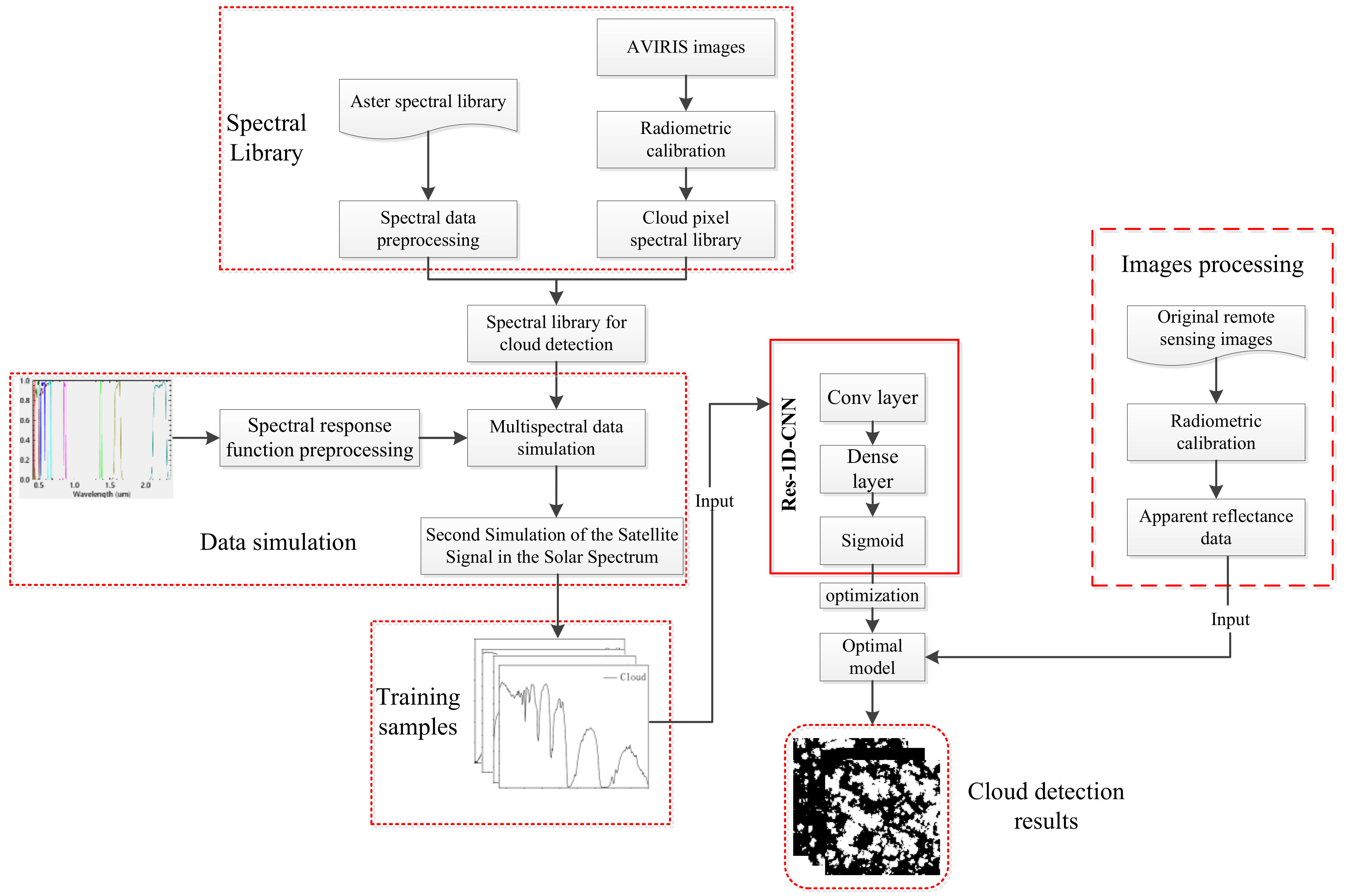
Figure 1 presents the detailed framework of the proposed algorithm. The CD-SLCNN algorithm consists of three main steps: the establishment of a spectral library, data simulation and cloud detection, which are both based on residual learning, and the one-dimensional CNN (Res-1D-CNN). The spectral library for cloud detection includes both the Advanced Spaceborne Thermal Emission Reflection Radiometer (ASTER) library [30] and cloud pixel spectrum library. The ASTER spectral library contains a comprehensive collection of spectra and is selected as the typical feature spectral library, the details of which will be provided in Section 2.1.1. The Airborne Visible/Infrared Imaging Spectrometer (AVIRIS) data, with a 0.4–2.5 µm continuous wave band, were used to establish a cloud pixel library, which can be utilised to explore slight differences between clouds and ground features [31]. The pixel dataset consisting of the ASTER spectral library and cloud pixel spectral library was converted to a multispectral version dataset based on the sensor spectral response function (SRF) and Second Simulation of the Satellite Signal in the Solar Spectrum (6S) model [32]. Cloud detection for different satellite remote sensing images, such as Landsat-8, MODIS, andSentinel-2, can be conducted using a shared set of spectral libraries, without requiring a new dataset. Finally, the Res-1D-CNN used as the classifier was applied in order to automatically learn and extract pixel spectral information and accurately detect the differences between clouds and ground features.
The remainder of the paper is organised as follows: Section 2 describe the details of the proposed method, Section 3 illustrates the experimental results and analysis, and Section 4 provides the overall summary of this study.

2. Method

2.1. Establishment of the Spectral Library

The spectral library for cloud detection includes the surface spectral feature and cloud spectrum. Different objects typically have unique spectral properties. Figure 2 shows the spectra of clouds and typical surface features. The primary difference between clouds and most ground objects is the reflectance in the visible light to the near-infrared range. The spectral library including clouds and large number of ground objects was used as the training dataset for the CD-SLCNN algorithm proposed in this study. Therefore, a representative spectral library was first established to provide abundant data samples to train the cloud detection network. The cloud detection spectral library contains the ASTER spectral library and the cloud pixel spectral library, and the details of these are described in Section 2.1.1 and Section 2.1.2.

2.1.1. ASTER Spectral Library

The ASTER spectral library (http://speclib.jpl.nasa.gov/, accessed on 18 August 2021) includes spectra of more than 2400 natural and artificial materials and was released on 3 December 2008. The library contains data from three other spectral libraries: the Johns Hopkins University Spectral Library (JHU), the Jet Propulsion Laboratory Spectral Library (JPL), and the United States Geological Survey Spectral Library (USGS). These spectra cover the entire visible infrared wavelength range (0.4–15.4 µm). The ASTER spectral library contains comprehensive spectra of ground objects over a wide spectral range. Therefore, it was selected as the ground object spectral library in this study. For cloud detection, considering the actual surface type, several rare minerals and lunar soils were removed from the ASTER spectral library. More than 1800 reflectance spectra of ground objects were used for cloud detection (i.e., non-cloud spectral samples).
The top of atmosphere (TOA) reflectance is an important parameter for cloud detection. ASTER library records the surface reflectance of different objects, which eliminates the atmospheric effect. Therefore, the 6S model was used to simulate the relationship between the apparent reflectance and surface reflectance under different observation and atmospheric conditions. The aerosol optical depth (AOD); geometric parameters, including solar zenith angle, observed zenith angle, and relative azimuth angle; atmospheric model; and aerosol type used in the 6S model are important factors affecting the simulation process. In order to account for all influencing factors in this study, the TOA reflectance of the objects in the ASTER spectral library was simulated for various geometric parameters (solar zenith, observed zenith, and relative azimuth angles); an AOD of 0.2, 04, 0.6, 0.8, and 1.0; three aerosol models (continental, oceanic, and urban); and different atmospheric patterns (midlatitude summer and winter). The number of final ground object spectra was 52,980.

2.1.2. Cloud Pixel Spectral Library

Hyperspectral remote sensing is a continuous imaging technology that acquires several narrow spectral channels, which can provide an approximate continuous spectral curve for each pixel in the image within the electromagnetic spectrum (e.g., visible light, near-infrared (NIR), short-wave infrared, and mid-infrared spectrum). The AVIRIS image with 224 continuous spectral channels is a major source of high-spectral-resolution images. The spectral range of AVIRIS images is 0.4–2.5 µm, wherein molecules and particles from terrestrial, aquatic, and atmospheric environments interact with solar energy through absorption, reflection, and scattering processes; therefore, this wavelength range is primarily used for cloud detection. AVIRIS images cover a wide range of land surface types, such as vegetation, urban areas, rivers, bare soil, snow, and glaciers [33,34,35]. However, a cloud pixel spectral library similar to the ASTER spectral library is not available. Therefore, 42 multi-temporal AVIRIS images with a 20 km spatial resolution were downloaded from https://aviris.jpl.nasa.gov/ (accessed on 18 August 2021) in order to build a high-quality cloud pixel spectral library. The 42 images were acquired in 2007–2018, covering the northeast, southeast, and southwest of the United States. These images contain several types of surfaces, such as vegetation, urban areas, ocean, and bare soil, as well as different cloud types, such as thick, thin, and broken clouds.
The AVIRIS images were radiometrically calibrated in order to obtain the TOA reflectance [36]. Considering the diversity of cloud states and effects of different surface types, thin clouds, thick clouds, broken clouds, and cloud edges, as well as the clouds over different types of underlying surfaces, such as vegetation, water, bright surfaces, and mountains, were manually selected. A total of 32,414 cloud pixels from 106 image blocks constitute the cloud pixel spectral library. A cloud pixel spectral sample comprises the TOA of all bands of each cloud pixel. Figure 3 shows typical examples of cloud pixels in different surface environments, including thick, thin, and broken clouds. Based on the spectra of clouds with different features, the reflectivity of thick clouds is higher than that of thin and broken clouds, and thin clouds have the lowest reflectivity. The TOA of clouds differs for different land surfaces. In particular, thin clouds are typically translucent, and most affected by the underlying surface.
The ASTER and cloud pixel spectral libraries constitute the spectral library for cloud detection based on CNN, with a total number of spectral samples of 85,394.

2.2. Data Simulation

The spectrum of ground objects in the ASTER library is the continuous reflection with a range of 0.4–15.4 µm, and the spectrum of cloud pixels from AVIRIS images represents the reflectance in the range of 0.4–2.5 µm. Our aim is to obtain the TOA of the sensor in the wide spectral range; hence, it is necessary to simulate the narrow-band ASTER spectral library and cloud pixel library from AVIRIS images in order to obtain a wide-band pixel library of the satellite data to be detected.
In this study, the ASTER and cloud pixel spectral libraries were used as the basis for data simulation. The relationship between hyperspectral and multispectral data was established based on the SRF of the sensor to be simulated. The simulation of the spectral library for multispectral data was performed in two stages: SRF pre-processing and spectral library simulation.

2.2.1. SRF Pre-Processing

The spectral range of objects in the ASTER spectral library is 0.4–15.4 µm, whereas the spectral range of clouds in the cloud pixel spectral library is 0.4–2.5 µm, and the spectral range of Landsat-8 OLI is 0.4–2.3 µm. Different spectral ranges indicate that the wavelength value of the spectral curve in the spectral library differs from that of the sensor SRF. Due to the fact that the spectral range of each object in the ASTER spectral library differs, the SRF should be linearly interpolated before data simulation so that it has the same wavelength as the spectral curve in the spectrum library used for convolution. As the spectral value interval in the SRF was 0.001, we adopted a convenient and effective linear interpolation method to process the SRF. After interpolation, each spectral curve in the spectral library had a set of corresponding SRFs.

2.2.2. Simulation of Spectral Library

Data simulation, converting the initial spectral library into a multispectral version of the spectral library, is a process of weighted synthesis based on the spectral response function (SRF) of the sensor to be detected. It was performed by converting the continuous TOA with a range of 0.4–15.4 µm into the TOA of the sensor in a wide spectral range. From an energy perspective, data simulation is a process of redistributing energy based on a known SRF, where the output energy of a multispectral band is interrelated to its spectral response and the spectral energy corresponds to the wavelength range of hyperspectral data [12]. Different sensors used to generate remote sensing images have unique spectral characteristics, which are reflected by their spectral ranges and spectral responses. The data simulation of remote sensing images uses the source data of the subdivided spectral bands and the entire spectral range of the sensor to be simulated in order to quantify the simulation data with established spectral properties. In this paper, the spectral library consisting of ASTER library and cloud pixels library as data source was used to generate the spectral library of Landsat-8, MODIS, and Sentinel-2A data.
Based on the SRF of the sensor and the wavelength range of the hyperspectral data, the following Equation was used for the data simulation:
R i M = i = 1 N H R j × f j j = 1 N H f j , i = 1 , , N M
where N H is the number of channels of the hyperspectral sensor (the spectral range of different objects in the spectrum library is different), N M is the number of channels of the sensor to be simulated, R i M is the pixel reflectance value of the multispectral data, R j is the pixel reflectance value of the spectral library, and f j is the SRF of the multispectral sensor corresponding to the wavelength of the spectral library pixel.
Figure 4 shows the comparison of the TOA reflectance of the cloud pixels from the AVIRIS, Landsat-8 OLI, and MODIS images with the simulated multispectral data. The spectral curve shows that the changes in the reflectance of simulated data (Landsat-8 OLI and MODIS) are consistent with the changes in the AVIRIS image (Figure 4a,b). The spectrum of the simulated cloud pixel is highly similar to that of the actual cloud pixel from the multispectral image (Figure 4c,d), which indicates that the simulated data are reliable. Based on the simulation of the spectral library, the cloud detection in different sensor images did not require a new spectral library, which mitigated the limitations of training samples in deep learning methods.

2.3. Cloud Detection Based on the Res-1D-CNN

Most existing cloud detection methods based on CNN mostly depend on many samples annotated at the pixel-level for parameter tuning; however, sample collection is tedious, time-consuming, and expensive [37,38,39]. In contrast, 1D convolution (Conv 1D) [40] can be effectively applied to identify and analyse signal data with fixed-length periods, including audio signals, time series, and spectral sequences. In order to address the above problem, we designed a cloud detection network supported by Res-1D-CNN. The network used the spectral library as training data, performing detection on the pixel-level, rather than using the whole image. It then automatically learned and extracted spectral information, effectively distinguished cloud and clear-sky pixels, and automatically generated binary cloud detection masks through model prediction.

2.3.1. Network Structure

The cloud detection network consists of two parts (Figure 5): the residual block (Residua + Conv1D) and the dense layer.
Residual block: convolutional layers can automatically extract hidden features of data through convolution operations. The ability of shallow CNN to extract information is limited. Deeper networks have large number of layers and complex network structures and thus have more powerful feature learning and feature expression capabilities. However, under limited training sample conditions, the neural network has problems, such as degradation and gradient disappearance, owing to the increasing depth of the network, which implies that it is more difficult to train the network, and thus, more training errors occur. For a simpler and more effective training of the network, a residual learning unit is introduced to the cloud detection network. The basic concept of residual learning is to introduce a shortcut based on the traditional network structure. The connections that jump over several layers are directly added to the main path. Therefore, bottom layer errors in the training process can be propagated to the upper layer through crystallisation, which alleviates the gradient dispersion problem caused by large number of layers and simplifies the training of the deep networks. The cloud detection network includes three residual blocks, and each contains a dual-channel convolutional neural network and a convolutional layer with a convolution kernel size of 1 to introduce information from different layers. A dual-channel CNN consists of six convolutional layers, batch-normalisation, and rectified linear units (ReLU) activation function. The number of convolution kernels was 16, 32, and 64, for Block1, Block2, and Block3, respectively. The kernel size in each convolution layer of the dual-channel CNN was 3, and the step size was set to 1. The output of each block includes the features from a dual-channel CNN and the convolutional layer with the convolution kernel size of 1, which integrates the low-level and high-level information.
In the Conv 1D calculation process, the convolution kernel slides along the sequence in a certain order, moving to a fixed position each time. Then, the corresponding point value is multiplied and summed. The mathematical expression of 1D convolution can be expressed by Equation (2) as follows:
S ( n ) = ( f * g ) [ n ] = m = 0 N 1 f ( m ) g ( n m )
where f ( n ) is the initial spectrum sequence, g ( n ) is the convolution kernel, S ( n ) is the convolution result sequence, N is the length of the sequence f ( n ) , and m and n represents the m-th and n-th spectral values, respectively.
The input of the next layer is the output of the two paths of the previous layer, which can be obtained using Equation (3). The purpose of this process is the establishment of two paths to achieve a multi-channel flow of information to improve the effectiveness of the network.
x i + 1 = x i + f ( x i , w i ( 1 ) ) + f ( x i , w i ( 2 ) )
where x i is the input of the residual module; x i + 1 is the output of the residual module; f ( x i , w i ( 1 ) ) and f ( x i , w i ( 2 ) ) are the convolution results of the last convolution layer of each residual block of the dual convolution channel, respectively; and w i ( 1 ) and w i ( 2 ) are the convolution weights.
Dense layer: the dense layer is a “classifier” of the entire CNN, which maps the feature representation learned by the convolutional layers to the sample space. In the proposed network, three residual modules are followed by two dense layers. The number of neurons in the two dense layers is 128 and 2, respectively. The last dense layer with the sigmoid activation function obtained the probability of cloud or non-cloud.

2.3.2. Network Training

Cloud detection based on Res-1D-CNN is defined as a binary classification problem (cloud and non-cloud). Category judgement is performed for each pixel, and the binary classification cross entropy is selected as the loss function. The spectral sequence (TOA reflectance of ground objects and clouds in different bands) and corresponding sequence labels (cloud and non-cloud) are used as inputs for the network. The goal is to learn an optimal model by minimising the loss value in order to predict clouds in the remote sensing image. The residual learning and dual-channel CNN provide multi-level features for cloud and clear-sky pixel prediction. In order to minimise the prediction results and label errors, the adaptive moment estimation (Adam) optimiser and back propagation were used to dynamically adjust the model parameters with an initial learning rate of 0.001. To prevent overfitting, the dropout layer parameter was set to 0.5, which implies that 50% of the parameters were randomly reduced during the network training phase. The batch size of the network was 128. Finally, with the support of an Intel Xeon CPU E5-2620 (v4, 2.10 GHz), the cloud detection network was trained from the beginning using the cloud detection spectral library. When the number of learning reached 100, the training accuracy and loss were stabilised.

3. Experiment and Results

We conducted cloud detection experiments on Landsat-8, Terra MODIS, and Sentinel-2A data of different regions and at different times in 2013–2020. In these experiments, the total number of samples in the pixel library was 85,394, wherein the number of cloud pixels and ground object pixels were 32,414 and 52,980, respectively. Bands 2, 3, 4, 5, 6, 7, and 9 were used for Landsat-8 images, bands 1-7 for MODIS images and bands 2, 3, 4, 8, 11, and 12 for Sentinel-2A images. The initial spectral library was simulated as the cloud detection spectral library of Landsat-8, MODIS, and Sentinel-2A satellite images, respectively. The cloud detection neural network (described in Section 2.3) was used as the classifier to identify clouds and surface features. In addition, Landsat-8 cloud cover assessment validation data (Landsat-8 Biome) [41] and MOD35 cloud product [42] were used to validate the performance of the proposed algorithm qualitatively and quantitatively.
The Fmask algorithm, a widely recognised cloud detection algorithm, was used for the comparison [43,44]. Random forest (RF) and SVM classifiers, which are based on machine learning algorithms, were also used for comparison with the proposed method. The training data for RF and SVM were the same as that of the proposed method.

3.1. Detection Performance on Landsat-8 Data

For cloud detection, 62-scene Landsat-8 satellite images were used; 36-scene images with the approximate cloud percentage of 5–100% were from the Landsat-8 biome, and the other 26-scene images were randomly selected in the globe, which include not only different densities and sizes of clouds but also various land surfaces. The underlying surfaces of the validation data included barren land, grass/crops, forests, shrubland, urban areas, snow/ice, wetlands, and water bodies.
Figure 6 shows four typical cloud detection results of the Landsat-8 images, including vegetation, sand, mountains, towns, lakes, oceans, and other complex surface types. In each Landsat-8 image, the upper left part shows the false-colour composite image (RGB: bands 5, 4, and 3), and the upper right part displays the corresponding cloud detection results of the entire image, where the white and black parts represent the cloud and clear-sky pixels, respectively. For better comparisons of the cloud detection results with visual interpretations, the lower left and lower right parts of the images present the enlarged details of areas marked by yellow boxes in the upper left and upper right parts, respectively. From the comparison of the cloud detection results with the ground observations, the CD-SLCNN algorithm accurately and reliably identified most of the clouds in the image at different times and in different areas, revealing a large amount of underlying surface information. The CD-SLCNN algorithm performed well for the various cloud types and sizes over diverse environments. Thick, thin, and broken clouds were detected in the enlarged area in the lower right corner of (a), (b), (c), and (d) in Figure 6, and the cloud edges were completely extracted.
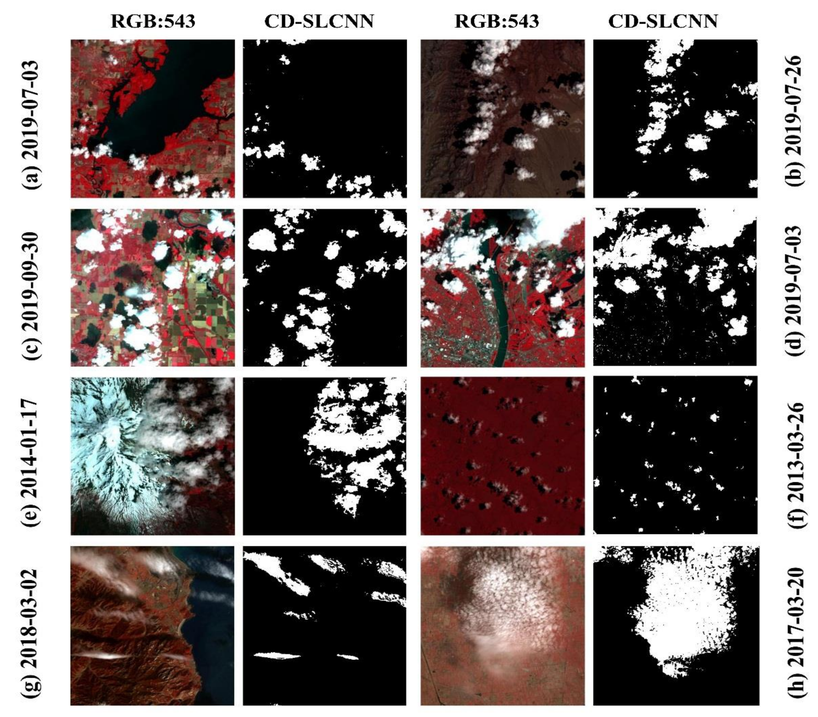
In order to better analyse the details and detection results, the images obtained over more challenging areas are shown. The left and right sides in Figure 7 show the Landsat-8 false-colour image (RGB: bands 5, 4, 3) and corresponding cloud detection result, respectively. In the cultivated land area (Figure 7c), the cloud detection results are not affected by the coverage with various crops, and the clouds were well distinguished. Furthermore, thin clouds over darker surfaces, such as inland water and oceans, can also be accurately identified (Figure 7h), suggesting acceptable classification results. Bright surfaces have similar spectral characteristics to clouds because of their high surface reflectance, particularly in the visible and NIR bands. This challenges traditional cloud detection approaches because it is difficult to determine an appropriate threshold and can lead to the misidentification of bright surfaces as clouds, as well as difficulties in accurately detecting thin clouds. The results presented in Figure 7b,d,g show that the CD-SLCNN algorithm can detect most clouds over bare soils, urban areas, and rocks, respectively, with few cloud omissions and false recognitions, particularly regarding thin and broken clouds. Due to the fact that the colour and reflectance of snow and ice are similar to those of clouds in visible bands, the recognition of cloud over these environments has always been a challenge in cloud detection. However, the CD-SLCNN algorithm uses Res-1D-CNN to deeply mine the spectral differences and hidden features of clouds and ice/snow in the near-infrared band in order to distinguish ice/snow and clouds and obtain cloud contours that are complete (Figure 7e). Small and broken clouds are typically omitted in cloud detection. However, the cloud detection results show that the CD-SLCNN algorithm efficiently recognised small and broken clouds well, with a good level of robustness. Notably, the performance of the CD-SLCNN algorithm is slightly inferior in urban areas with low vegetation coverage and bright buildings, with a small number of misidentifications of clear-sky pixels as clouds.
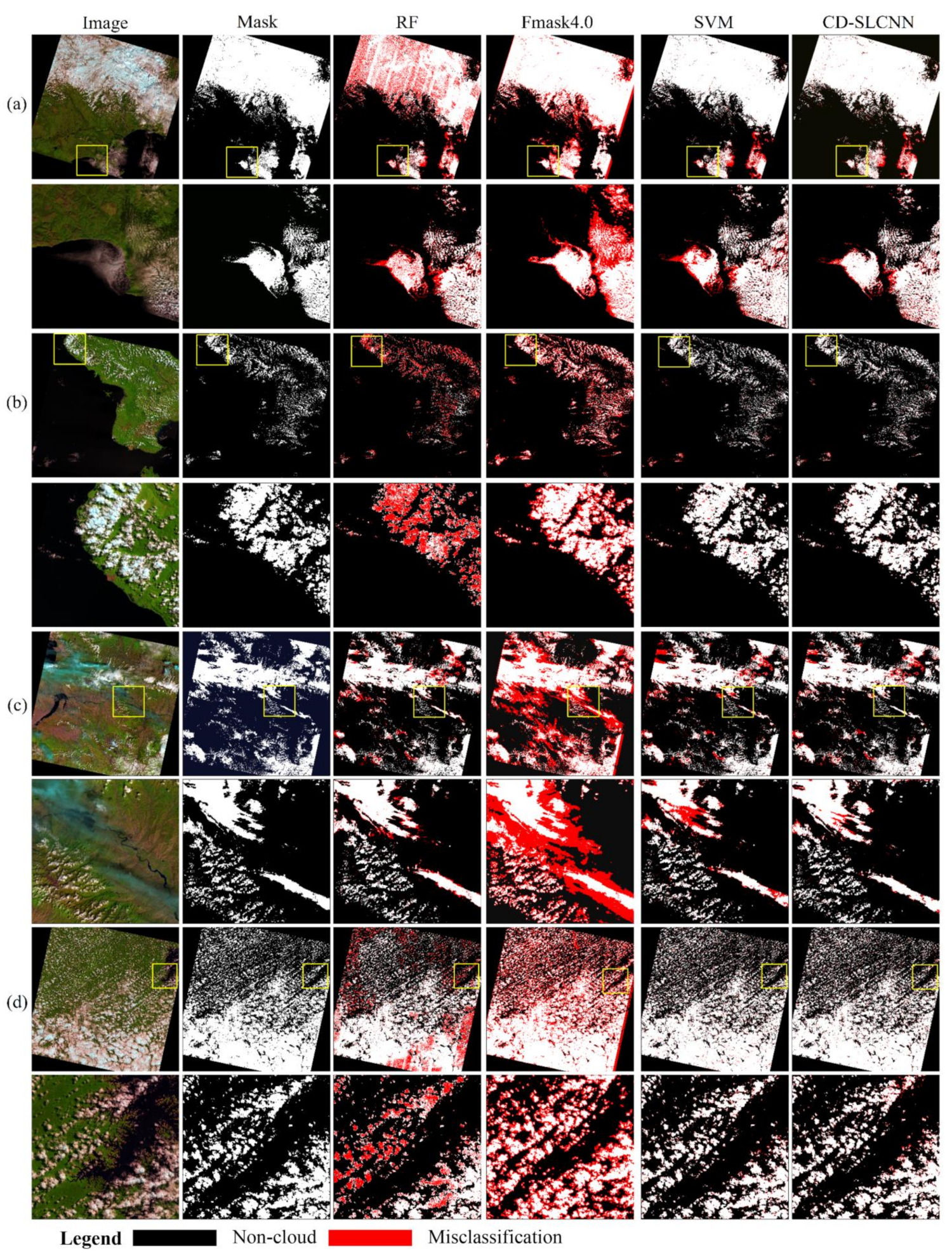
In order to further assess the effectiveness of the CD-SLCNN algorithm, the cloud extraction results from Fmask 4.0, RF, SVM, and our proposed method on 36-scene Landsat-8 biome images were compared with the manual cloud mask. These results are presented in Figure 8. In Figure 8, the first column displays the false-colour composite images (RGB: bands 6, 5, and 4); the second column displays the manual cloud mask; the third to sixth columns show the cloud detection results from RF, Fmask4.0, SVM, and our proposed method, respectively. The second, fourth, sixth, and eighth rows show the enlarged details of areas marked by red boxes in the first, third, fifth, and seventh row, respectively. In the third to sixth columns, white indicates that the results are consistent with the mask, red indicates the misclassification and less red indicates a better effect on cloud detection. The cloud extractions of the RF and Fmask 4.0 algorithm have significant differences with the cloud mask, which implies poor cloud recognition. For different underlying surfaces, there were various omission and commission errors. The results from SVM and the proposed method were similar to the cloud mask, and the overall detection was good. Furthermore, for clouds over water bodies and thin clouds, the CD-SLCNN algorithm performed better than SVM. The CD-SLCNN algorithm can extract deep information, which produces accurate and stable detection results. Nevertheless, the cloud cover areas detected using our method exhibited a high consistency with the cloud mask, indicating promising results. There were fewer misclassified cloud pixels in our results than those obtained using competing methods, as observed in the enlarged images in the yellow rectangles in Figure 8.

3.2. Detection Performance on MODIS and Sentinel-2 Data

MODIS data have been widely used for cloud detection. The MODIS cloud mask (MOD35) is a representative cloud detection product. In this experiment, 25-scene Terra MODIS 1B images and the corresponding MOD35 cloud product were used. Furthermore, 20-scene Sentinel-2A images were also applied to the validation.
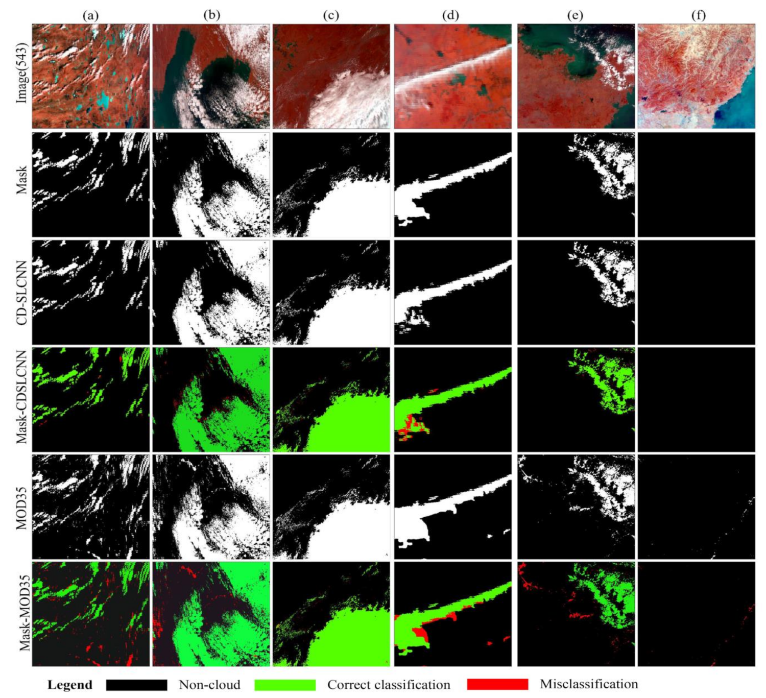
Figure 9 shows the cloud detection results for the MODIS data over diverse underlying surfaces. The first row presents false-colour images that were synthesised using bands 5, 4, and 3; the second row shows the manual cloud mask; the third and fifth rows display cloud detection results and the MOD35 cloud mask, respectively; the fourth and the last rows show the misclassification of the CD-SLCNN results and the MOD35 cloud mask, respectively. Green denotes the consistency with the manual cloud mask and red implies misclassification (e.g., objects identified as clouds or clouds identified as objects) in the cloud detection results of the CD-SLCNN and MOD35 cloud mask. These results indicated that the CD-SLCNN algorithm can effectively identify clouds over soil, vegetation, urban areas, and water bodies with fewer misclassifications. Based on the abundant features obtained by CNN, the CD-SLCNN algorithm could effectively distinguish the surface, as well as thick, thin, and broken clouds.
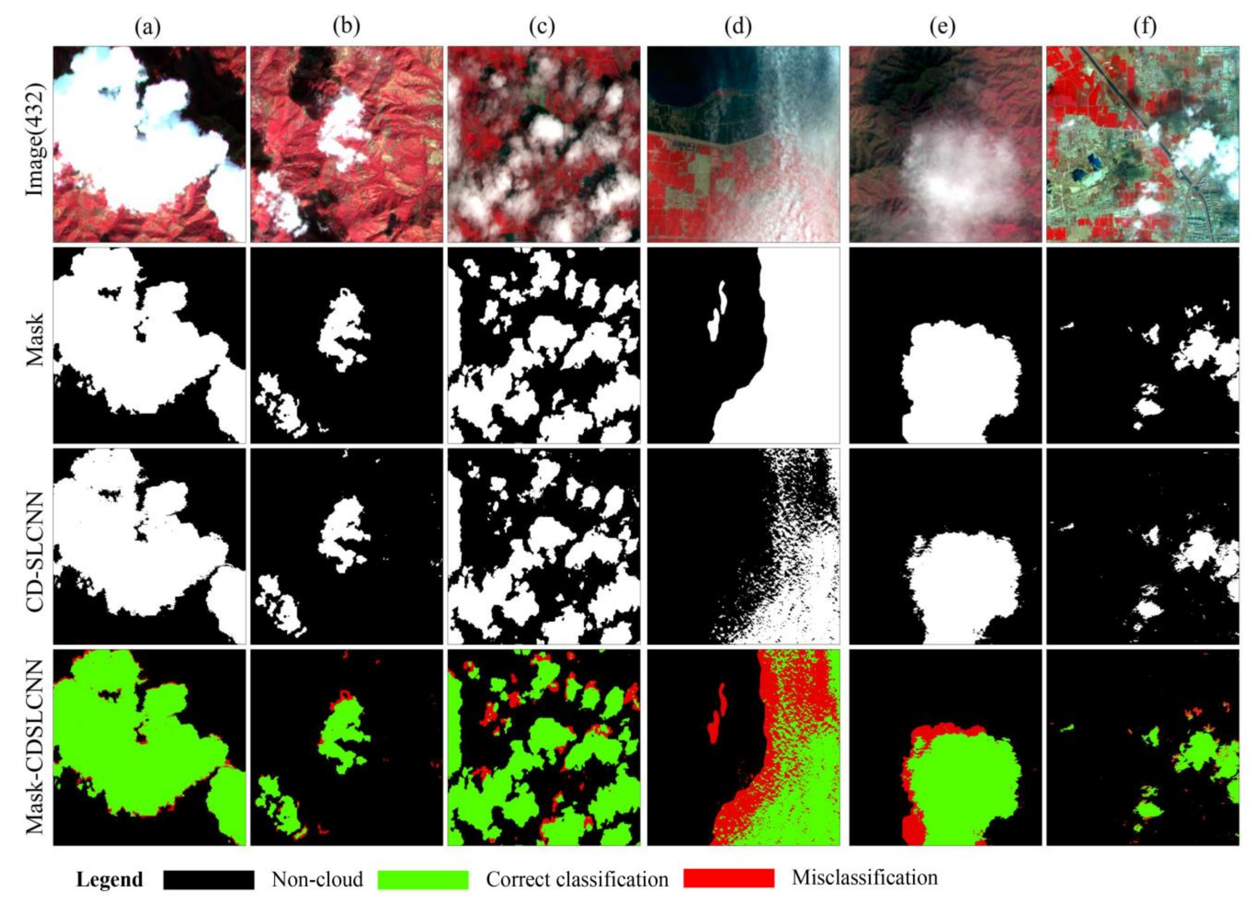
Figure 10 presents the cloud detection results for Sentinel-2A data, including thick clouds (thick and bright white, Figure 10a–c), thin clouds (thin and translucent, Figure 10d,e), and broken clouds (small size, and irregular shapes, Figure 10c,f). The first row shows false-colour images synthesised using bands 8, 4, and 3; the second row shows the manual cloud mask; the third and the last rows display cloud detection results and the difference in the CD-SLCNN results with the manual cloud mask, respectively. Green denotes the consistency with the manual cloud mask, whereas red denotes the inconsistency. The proposed algorithm performed well on thick clouds with subtle differences. The extraction results on thin clouds and broken clouds were slightly inferior, however, a recognition accuracy of 80% and above was achieved.
The interpretation and analysis that were conducted to validate the three datasets indicate that the CD-SLCNN algorithm proposed in this study was suitable for multi-satellite remote sensing images and achieved a good performance for diverse underlying surfaces. The detection of thin and broken clouds has also been improved. In Section 3.3, the quantitative analysis of cloud detection results is described.

3.3. Quantitative Analysis

3.3.1. Landsat-8 Biome

This study used 36-scene Landsat-8 biome images for quantitative verification. The cloud mask of the Landsat-8 biome was used as reference data to evaluate the accuracy of the cloud detection results from RF, SVM, and the proposed algorithm. The mean intersection over union (MIoU), kappa coefficient (Kappa), overall accuracy (OA), producer accuracy (PA), user accuracy (UA), and F1-score were used to quantitatively evaluate the proposed CD-SLCNN method.
Table 1 shows that the CD-SLCNN method was better than the competing methods in terms of OA, UA, MIoU, and Kappa. Our proposed method was advantageous in terms of Kappa (84.27%) and had the highest OA (95.60%), UA (96.43%), and MIoU (77.82%) accuracies among all competing methods.

3.3.2. MODIS and Sentinel-2

Herein, 25-scene Terra MODIS 1B images and 20-scene Sentinel-2A images were quantitatively evaluated. Table 2 and Table 3 present the quantitative validation results of the different methods. From Table 2 and Table 3, we observed that the proposed method achieved an outstanding cloud detection performance on MODIS and Sentinel-2 data. The OA, Kappa, and MIoU for cloud detection on MODIS images were 95.36%, 83.78%, and 77. 94%, respectively. This implies that the proposed method exhibited a high performance in detecting clouds over diverse underlying surfaces.
Table 3 suggests that good results were obtained for the Sentinel-2A images with an OA of >94% and Kappa of >80%. The high PA value (91.61%) implies that most of the clouds in the Sentinel-2A images can be well recognised. The UA (96.84%) demonstrated that there were fewer misclassifications. The recognition of thin clouds was slightly inferior to thick clouds due to the translucency and unclear boundaries of thin clouds.

3.4. Discussion

Qualitative and quantitative evaluations show that the proposed algorithm performed well in terms of the cloud detection for various types of remote sensing images. In order to ensure the wide application of the algorithm in multi-satellite remote sensing images, multispectral data simulation technology was adopted. In order to minimise the errors from the data simulation, all of the possible influencing factors, such as the atmospheric model, aerosol type, and AOD, were considered. Moreover, abundant spectral samples and deep CNN models further promote high-precision cloud detection. Compared with traditional machine learning algorithms, deep learning models have incomparable nonlinear function approximation capabilities and can extract and express data features well. The combination of the data simulation and deep learning model provides a promising strategy for cloud detection for various types of satellite data. The cloud detection results on Landsat-8, MODIS, and Sentinel-2A fully demonstrate the robustness of the proposed algorithm.
Although the algorithm achieved automatic and efficient cloud detection, it has certain limitations. Spectral libraries and data simulation reduce the requirement for remote sensing interpretation and the influence of human subjectivity. However, they also ignore spatial information, which results in limited feature learning for complex scenes, such as a spectral information mixture of thin clouds and the ground surface, or the presence of bright underlying surfaces that may be easily confused with clouds. Achieving weakly supervised cloud detection from remote sensing images has attracted attention previously [45]. In future studies, we will explore the fusion of spectral and spatial information and propose unsupervised and high-precision cloud detection algorithms for multispectral remote sensing data.

4. Conclusions

For efficient and accurate cloud detection for various satellite images, a universal cloud detection algorithm (CD-SLCNN), which combines a spectral library and Res-1D-CNN, is presented in this paper. The algorithm was supported by the prior spectral library and data simulation. Data simulation technology based on SRF can rapidly obtain a spectral library of the sensor to be detected. A Res-1D-CNN model was used to perform automatic cloud detection by automatically learning and extracting features of cloud and clear-sky pixels, which reduced the effects of human-related factors. The CD-SLCNN method achieved cloud detection with a high accuracy on different types of multispectral images. The experimental results of Landsat-8, Terra MODIS, and Sentinel-2 images show that the proposed method performed well on different clouds types, sizes, and densities over different surface environments. Furthermore, compared with the Fmask cloud detection results, quasi-synchronous MODIS cloud mask products (MOD35), and the results of RF and SVM methods, the proposed method obtained the highest OA, Kappa, and MIoU, and the PA was higher by 2.81%, 3.2%, and 5.57% than the results of the SVM on the Landsat-8, MODIS, and Sentinel-2 data, respectively. The comparison demonstrated that the CD-SLCNN method produced a more accurate cloud contour for thick clouds, thin clouds, and broken clouds than the current methods. The dual-channel CNN and the information fusion between different layers enhanced the unique features that distinguish clouds from ground objects and enabled their comprehensive extraction. In some special scenes, such as ice and snow, the proposed method has also achieved good results with fewer misclassifications, which is of great significance for cloud detection over bright surface environments.
The CD-SLCNN algorithm is applicable to diverse sensor data and only requires SRFs of multispectral data, avoiding the time-consuming and labour-intensive manual labelling of vectors in order to establish the training dataset for various remote sensing data. In addition, the algorithm is highly automated, can process large remote sensing datasets in batches, and is simple to operate.

Author Contributions

Conceptualisation, N.M. and L.S.; methodology, L.S.; software, N.M.; validation, N.M., C.Z., and Y.H.; formal analysis, N.M.; investigation, N.M.; resources, L.S., C.Z., and Y.H.; funding acquisition, L.S., C.Z., and Y.H.; data curation, N.M.; writing—original draft preparation, N.M.; writing—review and editing, N.M., L.S., C.Z, and Y.H. All authors have read and agreed to the published version of the manuscript.

Funding

This research was funded by National Natural Science Foundation of China, grant number 41171408, 41976184; the Natural Science Foundation of Shandong Province, grant number ZR201702210379.

Acknowledgments

The authors thank the Earth Explorer of the United States Geological Survey for providing the Landsat-8 cloud cover validation dataset and also thank Z. Zhu and C.E. Woodcock for developing the Fmask algorithm and providing the codes. We would also like to thank the editors and reviewers for their constructive comments to improve the paper’s quality.

Conflicts of Interest

The authors declare no conflict of interest.

References

  1. Wei, J.; Huang, W.; Li, Z.; Sun, L.; Zhu, X.; Yuan, Q.; Liu, L.; Cribb, M. Cloud detection for Landsat imagery by combining the random forest and superpixels extracted via energy-driven sampling segmentation approaches. Remote Sens. Environ. 2020, 248, 112005. [Google Scholar] [CrossRef]
  2. Yang, J.; Guo, J.; Yue, H.; Liu, Z.; Hu, H.; Li, K. CDnet: CNN-Based Cloud Detection for Remote Sensing Imagery. IEEE Trans. Geosci. Remote Sens. 2019, 57, 6195–6211. [Google Scholar] [CrossRef]
  3. Li, X.; Zheng, H.; Han, C.; Zheng, W.; Chen, H.; Jing, Y.; Dong, K. SFRS-Net: A Cloud-Detection Method Based on Deep Convolutional Neural Networks for GF-1 Remote-Sensing Images. Remote Sens. 2021, 13, 2910. [Google Scholar] [CrossRef]
  4. Sun, L.; Wei, J.; Wang, J.; Mi, X.; Guo, Y.; Lv, Y.; Yang, Y.; Gan, P.; Zhou, X.; Jia, C.; et al. A universal dynamic threshold cloud detection algorithm (UDTCDA) supported by a prior surface reflectance database. J. Geophys. Res. Atmos. 2016, 121, 7172–7196. [Google Scholar] [CrossRef]
  5. Wei, J.; Sun, L.; Peng, Y.; Wang, L.; Zhang, Z.; Bilal, M.; Ma, Y. An improved high-spatial-resolution aerosol retrieval algorithm for MODIS images over land. J. Geophys. Res. Atmos. 2018, 123, 12291–12307. [Google Scholar] [CrossRef]
  6. Zhang, Q.; Yuan, Q.; Li, Z.; Sun, F.; Zhang, L. Combined deep prior with low-rank tensor SVD for thick cloud removal in multitemporal images. ISPRS J. Photogramm. Remote Sens. 2021, 177, 161–173. [Google Scholar] [CrossRef]
  7. Sun, L.; Zhou, X.; Wei, J.; Wang, Q.; Liu, X.; Shu, M.; Chen, T.; Chi, Y. A New Cloud Detection Method Supported By GlobeLand30 Data set. IEEE J. Sel. Top. Appl. Earth Obs. Remote Sens. 2018, 11, 3628–3645. [Google Scholar] [CrossRef]
  8. Zhu, Z.; Woodcock, C.E. Automated cloud, cloud shadow, and snow detection in multitemporal Landsat data: An algorithm designed specifically for monitoring land cover change. Remote Sens. Environ. 2014, 152, 217–234. [Google Scholar] [CrossRef]
  9. Zhu, Z.; Wang, S.; Woodcock, C.E. Improvement and expansion of the Fmask algorithm: Cloud, cloud shadow, and snow detection for Landsats 4–7, 8, and sentinel 2 images. Remote Sens. Environ. 2015, 159, 269–277. [Google Scholar] [CrossRef]
  10. Ackerman, S.A.; Strabala, K.I.; Menzel, W.P. Discriminating clear sky from clouds with MODIS. J. Geophys. Res. 1998, 103, 32141–32157. [Google Scholar] [CrossRef]
  11. Frey, R.A.; Ackerman, S.A.; Liu, Y. Cloud detection with MODIS. Part I: Improvements in the MODIS cloud mask for collection 5. J. Atmos. Oceanic Technol. 2008, 25, 1057–1072. [Google Scholar] [CrossRef]
  12. Sun, L.; Yang, X.; Jia, S.; Jia, C.; Zhou, X. Satellite data cloud detection using deep learning supported by hyperspectral data. Int. J. Remote Sens. 2019, 41, 1349–1371. [Google Scholar] [CrossRef] [Green Version]
  13. Yuan, Q.; Shen, H.; Li, T.; Li, Z.; Zhang, L. Deep learning in environmental remote sensing: Achievements and challenges. Remote Sens. Environ. 2020, 241, 111716. [Google Scholar] [CrossRef]
  14. Hagolle, O.; Huc, M.; Pascual, D.V.; Dedieu, G. A multi-temporal method for cloud detection, applied to FORMOSAT-2, VENµS, LANDSAT and SENTINEL-2 images. Remote Sens. Environ. 2010, 114, 1747–1755. [Google Scholar] [CrossRef] [Green Version]
  15. Mateo-García, G.; Gómez-Chova, L.; Amorós-López, J.; Muñoz-Marí, J.; Camps-Valls, G. Multitemporal cloud masking in the Google Earth Engine. Remote Sens. 2018, 10, 1079. [Google Scholar] [CrossRef] [Green Version]
  16. Lyapustin, A.; Wang, Y.; Frey, R. An automatic cloud mask algorithm based on time series of MODIS measurements. J. Geophys. Res. 2008, 113, D16207. [Google Scholar] [CrossRef] [Green Version]
  17. Wieland, M.; Li, Y.; Martinis, S. Multi-sensor cloud and cloud shadow segmentation with a convolutional neural network. Remote Sens. Environ. 2019, 230, 111203. [Google Scholar] [CrossRef]
  18. Walder, P.; Maclaren, I. Neural network based methods for cloud classification on AV.HRR images. Int. J. Remote Sens. 2010, 21, 1693–1708. [Google Scholar] [CrossRef]
  19. Li, P.; Dong, L.; Xiao, H.; Xu, M. A cloud image detection method based on SVM vector machine. Neurocomputing 2014, 169, 34–42. [Google Scholar] [CrossRef]
  20. Chai, D.; Newsam, S.; Zhang, H.; Qiu, Y.; Huang, J. Cloud and cloud shadow detection in landsat imagery based on deep convolutional neural networks. Remote Sens. Environ. 2019, 225, 307–316. [Google Scholar] [CrossRef]
  21. Li, Z.; Shen, H.; Cheng, Q.; Liu, Y.; You, S.; He, Z. Deep learning based cloud detection for medium and high resolution remote sensing images of different sensors. ISPRS J. Photogramm. Remote Sens. 2019, 150, 197–212. [Google Scholar] [CrossRef] [Green Version]
  22. Guo, J.; Yang, J.; Yue, H.; Tan, H.; Hou, C.; Li, K. CDnetV2: CNN-Based Cloud Detection for Remote Sensing Imagery With Cloud-Snow Coexistence. IEEE Trans. Geosci. Remote Sens. 2021, 59, 700–713. [Google Scholar] [CrossRef]
  23. Ma, N.; Sun, L.; Wang, Q.; Yu, Z.; Liu, S. Improved cloud detection for landsat 8 images using a combined neural network model. Remote Sens. Lett. 2020, 11, 274–282. [Google Scholar] [CrossRef]
  24. Segal-Rozenhaimer, M.; Li, A.; Das, K.; Chirayath, V. Cloud detection algorithm for multi-modal satellite imagery using convolutional neural-networks (cnn). Remote Sens. Environ. 2020, 237, 111446. [Google Scholar] [CrossRef]
  25. Shao, Z.; Pan, Y.; Diao, C.; Cai, J. Cloud detection in remote sensing images based on multiscale features-convolutional neural network. IEEE Trans. Geosci. Remote Sens. 2019, 57, 4062–4076. [Google Scholar] [CrossRef]
  26. Ronneberger, O.; Fischer, P.; Brox, T. U-Net: Convolutional Networks for Biomedical Image Segmentation. Medical Image Computing and Computer-Assisted Intervention; Springer: Cham, Switzerland, 2015. [Google Scholar]
  27. Jeppesen, J.H.; Jacobsen, R.H.; Inceoglu, F.; Toftegaard, T.S. A cloud detection algorithm for satellite imagery based on deep learning. Remote Sens. Environ. 2019, 229, 247–259. [Google Scholar] [CrossRef]
  28. Francis, A.; Sidiropoulos, P.; Muller, J.P. Cloudfcn: Accurate and robust cloud detection for satellite imagery with deep learning. Remote Sens. 2019, 11, 2312. [Google Scholar] [CrossRef] [Green Version]
  29. Gómez-Chova, L.; Muñoz-Marí, J.; Amorós-López, J.; Izquierdo-Verdiguier, E.; Camps-Valls, G. Advances in synergy of AATSR-MERIS sensors for cloud detection. In Proceedings of the 2013 IEEE International Geoscience and Remote Sensing Symposium (IGARSS), Melbourne, VIC, Australia, 21–26 July 2013; pp. 4391–4394. [Google Scholar]
  30. Baldridge, A.M.; Hook, S.J.; Grove, C.I.; Rivera, G. The aster spectral library version 2.0. Remote Sens. Environ. 2009, 113, 711–715. [Google Scholar] [CrossRef]
  31. Sun, L.; Mi, X.; Wei, J.; Wang, J.; Tian, X.; Yu, H.; Gan, P. A cloud detection algorithm-generating method for remote sensing data at visible to short-wave infrared wavelengths. ISPRS J. Photogramm. Remote Sens. 2017, 124, 70–88. [Google Scholar] [CrossRef]
  32. Kotchenova, S.Y.; Vermote, E.F.; Matarrese, R.K.F., Jr. Validation of a vector version of the 6s radiative transfer code for atmospheric correction of satellite data, part i: Path radiance. Appl. Opt. 2006, 45, 6762–6774. [Google Scholar] [CrossRef] [Green Version]
  33. Vane, G.; Green, R.O.; Chrien, T.G.; Enmark, H.T.; Hansen, E.G.; Porter, W.M. The airborne visible/infrared imaging spectrometer (AVIRIS). Remote Sens. Environ. 1993, 44, 127–143. [Google Scholar] [CrossRef]
  34. Baugh, W.M.; Kruse, F.A.; Atkinson, W.W. Quantitative geochemical mapping of ammonium minerals in the southern cedar mountains, Nevada, using the airborne visible/infrared imaging spectrometer (AVIRIS). Remote Sens. Environ. 1998, 65, 292–308. [Google Scholar] [CrossRef]
  35. Wei, J.; Ming, Y.F.; Han, L.S.; Ren, Z.L.; Guo, Y.M. Method of remote sensing identification for mineral types based on multiple spectral characteristic parameters matching. Spectrosc. Spect. Anal. 2015, 35, 2862–2866. [Google Scholar]
  36. Thompson, D.; Gao, B.; Green, R.; Roberts, D.; Dennison, P.; Lundeen, S.; Mouradi, Y. Level 2 Processing of AVIRIS HyspIRI Preparatory Campaign Measurements. Available online: http://hyspiri.jpl.nasa.gov/downloads/2014_Symposium/day2/-0900_pres_HyspIRI_level2_140604c.pdf (accessed on 17 March 2014).
  37. Xie, F.; Shi, M.; Shi, Z.; Yin, J.; Zhao, D. Multilevel cloud detection in remote sensing images based on deep learning. IEEE J. Sel. Top. Appl. Earth Obs. Remote Sens. 2017, 10, 3631–3640. [Google Scholar] [CrossRef]
  38. Zhan, Y.; Wang, J.; Shi, J.; Cheng, G.; Yao, L.; Sun, W. Distinguishing cloud and snow in satellite images via deep convolutional network. IEEE Geosci. Remote Sens. Lett. 2017, 14, 1785–1789. [Google Scholar] [CrossRef]
  39. Shendryk, Y.; Rist, Y.; Ticehurst, C.; Thorburn, P. Deep learning for multi-modal classification of cloud, shadow and land cover scenes in PlanetScope and Sentinel-2 imagery. ISPRS J. Photogramm. Remote Sens. 2019, 157, 124–136. [Google Scholar] [CrossRef]
  40. Zhong, L.; Hu, L.; Zhou, H. Deep learning based multi-temporal crop classification. Remote Sens. Environ. 2018, 221, 430–443. [Google Scholar] [CrossRef]
  41. Foga, S.; Scaramuzza, P.L.; Guo, S.; Zhu, Z.; Dilley, R.D.; Beckmann, T.; Schmidt, G.L.; Dwyer, J.L.; Hughes, M.J.; Laue, B. Cloud detection algorithm comparison and validation for operational Landsat data products. Remote Sens. Environ. 2017, 194, 379–390. [Google Scholar] [CrossRef] [Green Version]
  42. Levy, R.C.; Mattoo, S.; Munchak, L.A.; Remer, A.; Sayer, M.; Hsu, N.C. The collection 6 MODIS aerosol products over land and ocean. Atmos. Meas. Tech. Discuss. 2013, 6, 159–259. [Google Scholar]
  43. Mateo-García, G.; Laparra, V.; López-Puigdollers, D.; Gómez-Chova, L. Transferring deep learning models for cloud detection between Landsat-8 and Proba-V. ISPRS J. Photogramm. Remote Sens. 2020, 160, 1–17. [Google Scholar] [CrossRef]
  44. Sun, L.; Liu, X.; Yang, Y.; Chen, T.; Wang, Q.; Zhou, X. A cloud shadow detection method combined with cloud height iteration and spectral analysis for landsat 8 oli data. ISPRS J. Photogramm. Remote Sens. 2018, 138, 193–207. [Google Scholar] [CrossRef]
  45. Zou, Z.; Li, W.; Shi, T.; Shi, Z.; Ye, J. Generative Adversarial Training for Weakly Supervised Cloud Matting. In Proceedings of the 2019 IEEE/CVF International Conference on Computer Vision (ICCV), Seoul, Korea, 27 October–2 November 2019; pp. 201–210. [Google Scholar]
Figure 1. Framework of the cloud detection algorithm based on a spectral library and a convolutional neural network (CD-SLCNN algorithm).
Remotesensing 13 03319 g001
Figure 2. Spectra of different objects: (a) spectrum of cloud; (b) spectrum of vegetation [30]; (c) spectrum of soil [30]; (d) spectrum of manmade surface [30]; (e) spectrum of snow/ice [30]; (f) spectrum of water [30].
Remotesensing 13 03319 g002
Figure 3. Spectra of thick, thin, and broken clouds in different surface environments. The red, green, and blue dots represent thick, broken, and thin clouds, respectively.
Remotesensing 13 03319 g003
Figure 4. Comparison of actual cloud pixel spectrum and simulated cloud pixel spectrum: (a) actual cloud pixel spectrum from AVIRIS image and simulated cloud pixel spectrum of Landsat-8; (b) actual cloud pixel spectrum from AVIRIS image and simulated cloud pixel spectrum of MODIS; (c) actual cloud pixel spectrum from Landsat-8 image and simulated cloud pixel spectrum of Landsat-8; (d) actual cloud pixel spectrum from MODIS image and simulated cloud pixel spectrum of MODIS.
Remotesensing 13 03319 g004
Figure 5. Network structure of cloud detection algorithm. Block1, Block2, and Block3 represent three identical residual modules. Each block contains residual learning (Conv 1D, 1) and a dual-channel convolutional network.
Remotesensing 13 03319 g005
Figure 6. Examples of false-colour (RGB: bands 5, 4, and 3) composite images and cloud (masked white) detection results for Landsat-8 full-scene and enlarged-in images (areas outlined by yellow boxes) over diverse underlying surfaces: (a) vegetation and inland water areas, acquired on 3 July 2019, at Path 23 and Row 33; (b) bare soil areas, acquired on 29 July 2019, at Path 40 and Row 34; (c) ocean, sand, vegetation, and urban areas, acquired on 20 May 2017, at Path 118 and Row 38; (d) vegetation and urban areas, acquired on 30 June 2019, at Path 123 and Row 32.
Remotesensing 13 03319 g006
Figure 7. Examples of false-colour composite images and cloud (masked as white) detection results for Landsat-8 subimages over diverse underlying surfaces: (a) vegetation and inland water areas; (b) bare soil areas; (c) cultivated land areas; (d) urban area areas; (e) snow/ice areas; (f) vegetation areas; (g) rock and ocean areas; (h) vegetation and urban areas. The annotations on the left and right sides indicate the acquisition time.
Remotesensing 13 03319 g007
Figure 8. Comparison of the Mask, RF, Fmask4.0, SVM, and CD-SLCNN cloud detection results on Landsat-8 biome for: (a) forest and ocean areas, acquired on 26 August 2014, with a center longitude at 149° E and a center latitude at 60° N, at Path 108 and Row 18; (b) urban and ocean areas, acquired on 29 August 2014, with a center longitude at 121° E and a center latitude at 4° S, at Path 113 and Row 63; (c) cultivated land areas, acquired on 31 August 2013, with a center longitude at 101° E and a center latitude at 36° N, at Path 132 and Row 35; (d) forest and inland water areas, acquired on 21 May 2014, with a center longitude at 56° W and a center latitude at 4° N, at Path 229 and Row 57.
Remotesensing 13 03319 g008
Figure 9. Qualitative comparison of cloud detection results in MODIS images over diverse underlying surfaces: (a) vegetation and inland water areas, acquired on 15 January 2013; (b) ocean areas, acquired on 8 October 2018; (c) forest areas, acquired on 29 December 2017; (d) vegetation and ocean areas, acquired on 8 October 2018; (e) ocean areas, acquired on 9 October 2018; (f) mountain and building areas, acquired on 28 November 2016.
Remotesensing 13 03319 g009
Figure 10. Qualitative comparison of cloud detection results in Sentinel-2A images over diverse underlying surfaces: (a) forest areas, acquired on 21 January 2020; (b) shrubland areas, acquired on 20 April 2019; (c) grass and island water areas, acquired on 27 July 2020; (d) urban and ocean areas, acquired on 23 March 2020; (e) bare soil areas, acquired on 23 March 2020; (f) urban areas, acquired on 30 March 2020.
Remotesensing 13 03319 g010
Table 1. Quantitative analysis of the CD-SLCNN results of Landsat-8 biome data.
MethodOAPAUAKappaMIoU
RF93.90%77.82%91.30%79.20%71.80%
Fmask92.71%92.78%79.59%82.16%77.53%
SVM95.26%80.40%94.82%83.50%77.44%
CD-SLCNN95.60%83.21%96.43%84.27%77.82%
Table 2. Quantitative analysis of the CD-SLCNN results of MODIS data.
MethodOAPAUAKappaMIoU
RF90.46%88.76%92.15%78.56%71.35%
MOD3592.44%85.24%99.63%80.16%74.75%
SVM93.32%88.96%98.07%83.08%77.40%
CD-SLCNN95.36%92.16%98.74%83.78%77.94%
Table 3. Quantitative analysis of the CD-SLCNN results of Sentinel-2 data.
MethodOAPAUAKappaMIoU
RF90.05%83.29%97.52%72.46%70.12%
SVM92.44%86.04%96.91%80.39%76.29%
CD-SLCNN94.27%91.61%96.84%81.17%77.23%
Publisher’s Note: MDPI stays neutral with regard to jurisdictional claims in published maps and institutional affiliations.

