
Fog Measurements with IR Whole Sky Imager and Doppler Lidar, Combined with In Situ Instruments


1
Environmental Physics Department, Israel Institute for Biological Research (IIBR), Ness Ziona 7410001, Israel
2
Life Science Research Israel (LSRI), Ness Ziona 7410001, Israel
*
Author to whom correspondence should be addressed.
Remote Sens. 2021, 13(16), 3320; https://0-doi-org.brum.beds.ac.uk/10.3390/rs13163320
Submission received: 20 July 2021
/
Revised: 18 August 2021
/
Accepted: 20 August 2021
/
Published: 22 August 2021
(This article belongs to the Section Atmospheric Remote Sensing)
Abstract
:This study describes comprehensive measurements performed for four consecutive nights during a regional-scale radiation fog event in Israel’s central and southern areas in January 2021. Our data included both in situ measurements of droplets size distribution, visibility range, and meteorological parameters and remote sensing with a thermal IR Whole Sky Imager and a Doppler Lidar. This work is the first extensive field campaign aimed to characterize fog properties in Israel and is a pioneer endeavor that encompasses simultaneous remote sensing measurements and analysis of a fog event with a thermal IR Whole Sky Imager. Radiation fog, as monitored by the sensor’s field of view, reveals three distinctive properties that make it possible to identify it. First, it exhibits an azimuthal symmetrical shape during the buildup phase. Second, the zenith brightness temperature is very close to the ground-level air temperature. Lastly, the rate of increase in cloud cover up to a completely overcast sky is very fast. Additionally, we validated the use of a Doppler Lidar as a tool for monitoring fog by proving that the measured backscatter-attenuation vertical profile agrees with the calculation of the Lidar equation fed with data measured by in situ instruments. It is shown that fog can be monitored by those two, off-the-shelf-stand-off-sensing technologies that were not originally designed for fog purposes. It enables the monitoring of fog properties such as type, evolution with time and vertical depth, and opens the path for future works of studying the different types of fog events.
1. Introduction
Fog is defined as a suspension of small, usually microscopic, water droplets in the air, reducing the visibility at the earth’s surface to a range of less than 1 km [1]. It affects many human activities, such as ground and aviation transport, and severely limits the performance of surveillance with electro-optical sensors. Characterization of fog properties is essential for realistic modeling of its physical behavior and estimation of its impact. In situ measurements of fog events provide essential data about the local fog density, droplets size distribution, surface-level temperature, relative humidity, and winds. However, they do not provide information about the fog’s vertical and horizontal extent. Moreover, they do not fully monitor the evolution patterns of fog events. Due to these limitations, in situ measurements lack the ability to provide sufficient information regarding limitations that fog poses to optical sensors performance in a range of spectral bands (e.g., visible to infrared (IR) passive sensors, laser and light-emitting diodes, etc.). Examining the performance of electro-optical tools inside the fog is an important and broad research area, covering, among other tools, Lidar (Light Detection and Ranging). To the best of our knowledge, this is the first research to explore whether and how IR Whole Sky Imagers (WSI) can provide additional information that may enhance our understanding and characterization of fog events.
Between 3–6 January 2021, for four mornings in a row, regional-scale dense fog spread over Israel’s central and southern areas. The heavy fog descended on large areas, blanketing towns, reducing visibility for drivers, and covering buildings.
Fog in Israel [2] generally sets in after midnight and persists until three to four hours after sunrise. In extreme cases, fog cover lingers for more than 10 h. There are several types of fog, two of them, advection fog and radiation fog, are the most common in Israel.
Advection fog occurs when moist air passes over a cool surface by advection and is cooled. It is most common at sea when moist air encounters cooler waters. A strong enough temperature difference over water or bare ground can also cause advection fog. In Israel, the advection fog can be seen during the spring season. The fog is created when the sea is cold and the nights are stable. In the morning it can be advected inland.
Radiative fog occurs when weather conditions are somewhat stable, usually when the ground is cold, as it occurs on long winter nights, and the wind speed is low. In addition, a dry layer must exist above the sea wind. The humidity prevents radiative cooling of the marine layer. Air pollution can be another contributing factor to heavy fog. The more polluted air helps to trap water drops and intensifies the fog.
In Israel, these radiative fog conditions are possible during the following synoptic regimes [3]:
a. Upper anticyclone—causes subsidence and dryness, which stimulate a breeze circulation. When the pressure gradient is not very strong, sea winds bring moist air which may cause fog.
b. A shallow anticyclone behind a cold front—causes quick stabilization during long winter nights.
c. The collapse of the cold front—similar to (b) but more common during transitional seasons than in winter. In these cases, the near-surface humidity accumulation causes thick fog, in the coastal plain.
d. Before a sharav depression—an easterly or southeasterly flow towards the depression. Exists in transitional seasons.
e. Red-Sea through (RST)—The RST is a break from the Sudan low residing in the intertropical convergence zone. The counterclockwise easterly or southeasterly flow dries the air. As described by Goldreich [2], the conditions are common to transitional seasons but can happen also in summer and winter. It can be classified into inactive or active RST depending on the weather’s upper subsidence or through accompanying it. The RST was further classified into wide and narrow. The wide RST is situated in southern Israel and is characterized by prevailing easterly winds. The narrow or sharp-edged RST was furtherly classified according to the location of its axis: an eastern RST with an axis east of Israel and westerly winds or a western RST with its axis west of Israel and easterly flow.
The automatic semi-objective classification of synoptic weather following Alpert et al. [4] classifies the present event as RST with an eastern axis for the 3rd of January and RST with a western axis for the 4th–6th of January.
The Israel Meteorological Service (IMS) published a special review of the rare fog event [5], stating that this was an unusual meteorological phenomenon during the winter months. According to this survey, it was a radiation fog triggered by the unseasonable weather that Israel was experiencing.
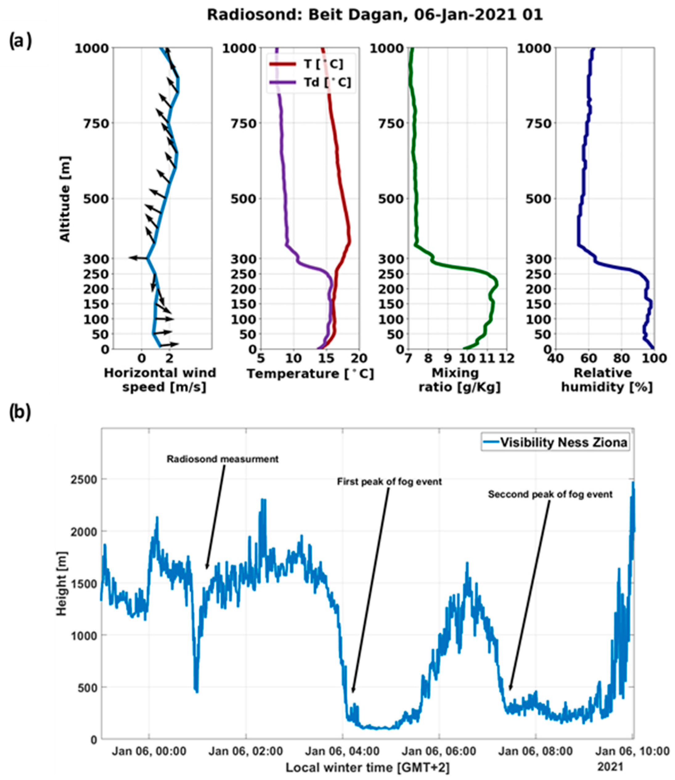
In a separate paper (in progress), we will describe mesoscale aspects of the January fog event through model simulations and will present measurements of meteorological and microphysical parameters. A needed parameter for active remote sensing applications is the fog vertical depth. The buildings in Figure 1 reach a height of up to 200 m above ground level, thus the vertical extent of the fog there is several meters below that height. The fog layer depth can be deduced also from a profile of radiosonde measurements. Figure 2a presents radiosonde results, launched by the IMS during the early morning of 6 January, including wind speed and direction, air and dew point temperatures, mixing ratio and relative humidity.
Figure 2b shows the visibility range that we measured during the same night, noting with arrows the fog periods where visibility was reduced to less than 1 km. Visibility range values during the radiosonde launching are close to the definition of fog visibility range threshold and thus can be used to describe the fog depth. The radiosonde data presents the humidity conditions that prevailed before and after the fog events. The fog built up later when temperature values decrease. The radiosonde shows relative humidity levels that were above 95% up to an altitude of 254 m. Above this height, the atmosphere became dryer with decreasing relative humidity values, dew point temperature and air temperature diverging, and a decrease in water-vapor mixing ratio. This transition height is the bottom of a second inversion layer ending at a height of 492 m. Horizontal wind speed values do not exceed 2 m/s under the inversion and wind direction changes at a height of 200–250 m. We assume that this approximately 200 m thick layer also determines the thickness of the fog layer.
Due to our deployed sensors, we were able to include various monitoring instruments to perform a comprehensive study during the fog event. We made continuous measurements with a wide variety of ground-based measurement tools. This assembly includes both in situ measurements and remote sensing instruments. The in situ instruments are conventional equipment for such measurements and provide observations of a collection of meteorological parameters, the size distribution of fog droplets, and visibility range. The more sophisticated and unique measurements were ground-based remote sensing with a Doppler Lidar and thermal IR WSI.
The use of a thermal IR WSI can be considered a pioneering endeavor in the context of fog characterization. To the best of our knowledge (we have not found any previously published scientific works that refer specifically to the characterization of fog events with WSI) this is the first time that a thermal IR WSI is used as a tool for describing the process of fog formation and dissipation. It is not surprising, since the ultimate goal of these instruments is to provide information about the cloud cover, and fog conditions either interfere or are conventionally monitored with alternative ground measurements. WSI in the thermal IR band is still very rare and still considered a relatively new technique. The only reference that we are aware of, is the intention of one of the manufacturers of the sky camera, ReuniWatt, to develop a tool to identify the occurrence of fog events [7]. Therefore, our measurements may open a path for employing IR WSI for the characterization of fog events.
Contrary to the sky imager, vertical Lidars are a common and well-known tool for observing the atmospheric profile. Fog is relevant in vertical Lidar measurements in two different aspects. First, as interference for measurement of a clean upward profile, (see for example in [8]).
The other application uses the Lidar potential to analyze fog properties, as for example in the work of Gultepe, et al., who presented measurements of Doppler Lidar to characterize fog [9]. In the current work, we validate the use of a Doppler Lidar as a monitoring tool for fog events, by comparing the measured attenuated backscatter profile with the calculated one. We show that the Lidar equation, calculated based on surface-level measured droplets-size distribution, reproduces well the measured signal. This result demonstrates the ability of the Doppler Lidar to monitor fog without additional instruments.
Fog droplets that exist in the Lidar line-of-sight affect the returned signal. Extinction and attenuated backscatter coefficients depend on the fog concentration. Since fog, unlike clouds, develops on the surface, ground measurements of fog droplets-size distribution performed in parallel with the Lidar profile measurements enable us to calculate the expected attenuated backscatter Lidar profile. We show that combining ground measurements of droplets- size distribution allows a direct evaluation of the time-dependent Lidar equation, under the assumption of a constant vertical profile of these properties. No additional information is needed.
The purpose of the present work is to analyze and characterize the January 2021 fog event, through a careful analysis of the directly measured and retrieved data from all instruments. We will elucidate the relationships among all of the quantitative results. This analysis enables us to explore the effect of a well-defined fog event on the performance of electro-optical sensors and visibility limitations. However, we emphasize that we do not consider our sensing instruments and their data analysis as a comprehensive alternative for widely used fog monitoring techniques. To our view, it is an efficient complementary technique that can provide unique and valuable information about fog events that cannot be achieved in any other method. It should be also observed that this study is based on a one-time radiation fog event and therefore further analysis regarding future events is required.
2. Instrumentation and Derived Parameters
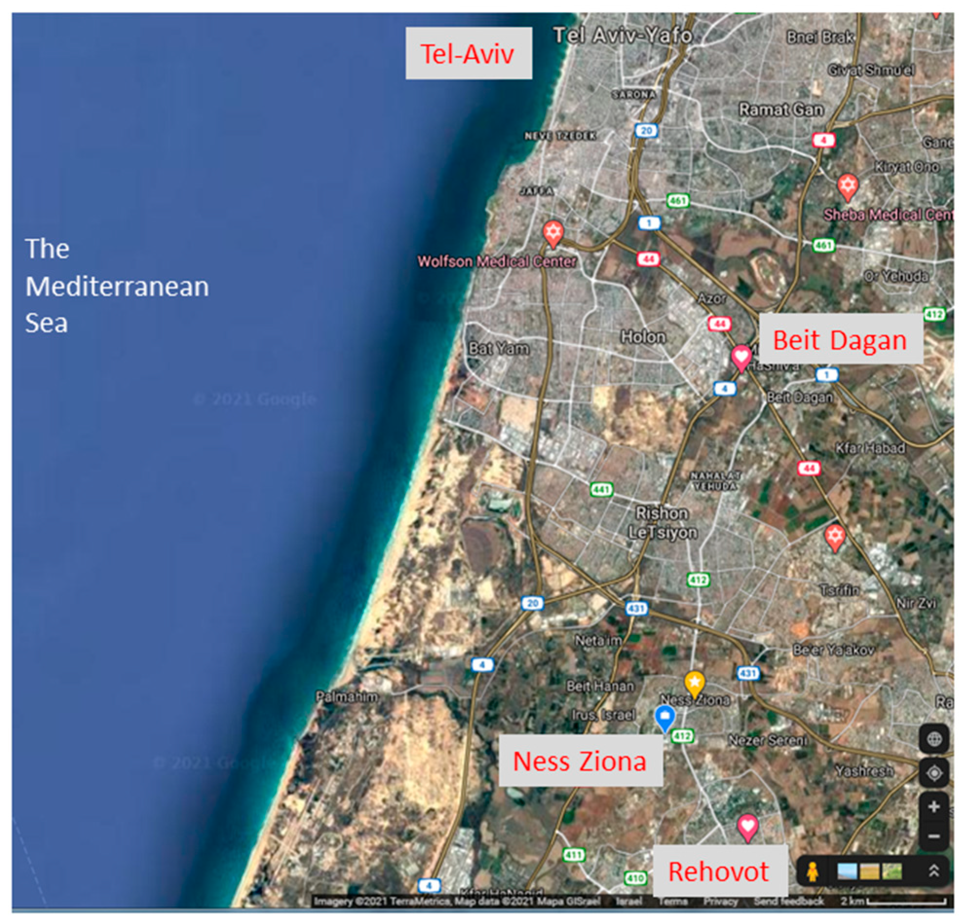
Our field campaign was held in Ness Ziona, Israel, during 3–6 January 2021. The location is about 8 km east of the Mediterranean Sea and is characterized by flat terrain (see Figure 3).
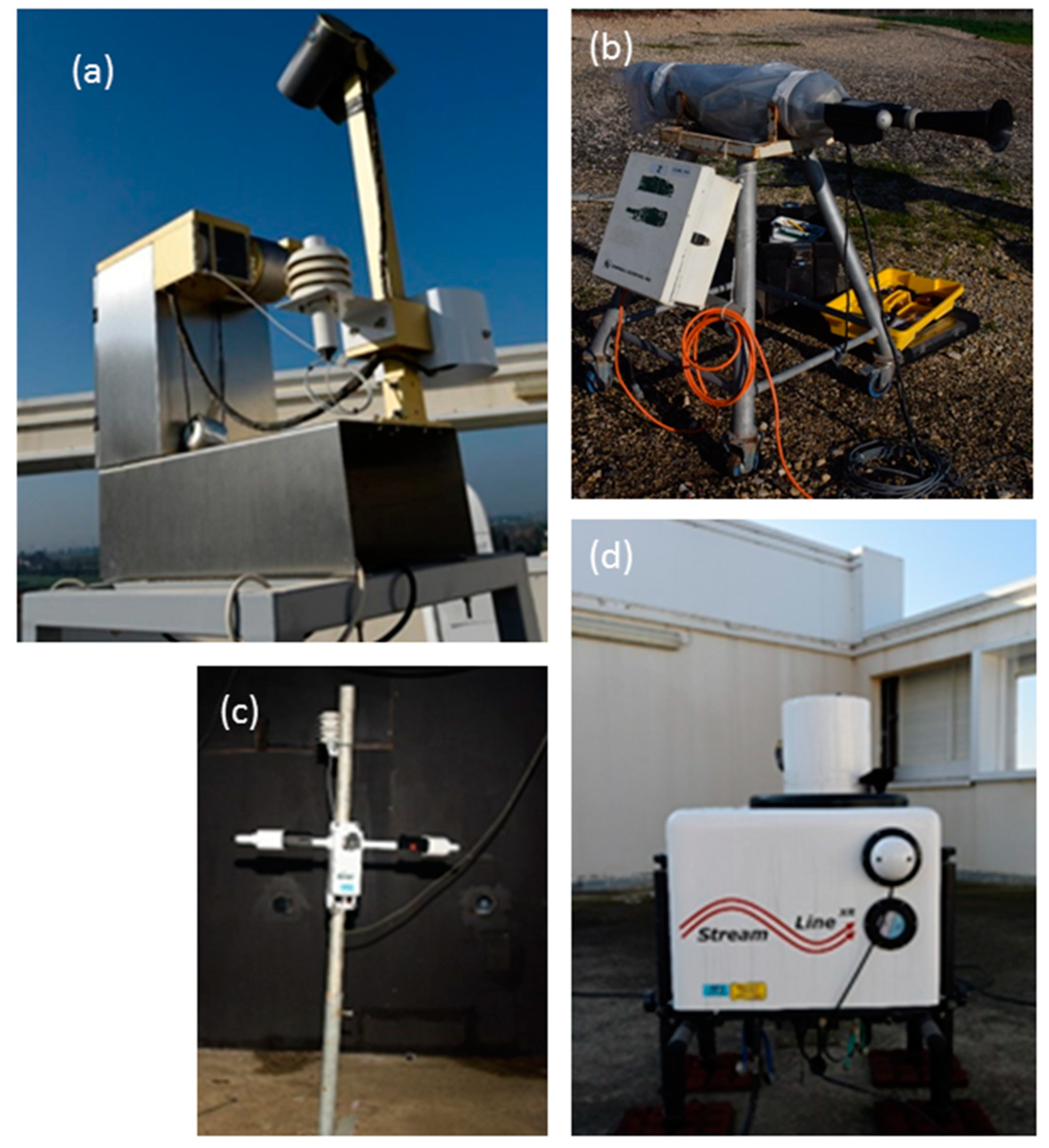
Several of the instruments were located in an open area on a hill that is 40 m above sea level, while others were on a nearby tall building roof at a similar height. The in situ meteorological measurements and remote sensing equipment are presented in Figure 4.
2.1. In Situ Measurement Sensors
2.1.1. Droplets Size Distribution
FSSP-100 [PMS, Boulder, Colorado, USA] is an optical Forward Scattering Spectrometer Probe used to measure online droplet size distribution in all-weather conditions. The spectrometer time resolution is 1 s. It was set in its lower scales to measure droplet sizes up to 16 microns and was pre-calibrated with a Flow Focusing Monodisperse Aerosol Generator 1520 [TSI, MN, USA].
The droplet size distribution allows calculation of the radiative-transfer properties of electro-optical waves based on the Mie scattering model [10], needed to describe the performance of sensors inside an aerosol medium. The mass-extinction coefficient σext [m−1] is defined as the fraction of attenuated energy per unit length, by weighing the Mie extinction efficiency, Qext, over the size-distribution function n(r), as follows:
where r is the fog droplet radius. Qext [11] depends on the sensor wavelength and the spectral dependence of the refractive index of water [12]. Similarly, β is the backscattering coefficient [m−1sr−1], defined with the backscatter efficiency Qb as follows:
Those two parameters will allow us to solve the Lidar equation, as will be shown in Section 3.2.
2.1.2. Visibility Range and Meteorological Data
An SWS250 [Biral, Bristol, UK] performed visibility range measurements. Humidity and temperature data were collected from the nearby local meteorological station “Rehovot”, maintained by the Israel Ministry of agriculture [13]. Humidity and radiosonde data were collected from “Beit Dagan” station that is maintained by the IMS [14]. Both stations are located no more than 10 km from the location of our facility and share the same climatological characterization (see locations in Figure 3).
2.2. Remote Sensing Techniques
2.2.1. Thermal IR and Visible WSI
Visible WSI is the most commonly known technique for ground-based cloud cover monitoring which is also highly effective for monitoring fog events during day time. However, they cannot operate properly under low light levels (such as at night time), and cannot yield quantitative physical parameters about the cloud. In recent years, IR WSI has appeared as an off-the-shelf product. Typical IR WSI contains an IR uncooled camera and it produces radiometrically calibrated images. The use of thermal imaging enables continuous 24/7 monitoring of the whole sky to obtain an unbiased and uninterrupted large dataset in order to study cloud cover dynamics and their characterization. Furthermore, as stated above, unlike visible range-based cameras, it enables the retrieval of important physical information about the cloud properties and the development of a well-established radiative transfer model of clear and cloudy atmospheres. This is due to the direct relationship between the radiometric signal obtained in the IR band and the cloud’s base height, opacity and total precipitable water along the line of sight (LOS). Shaw et al. (2005) [15] were the pioneers in this field, with the establishment of the technical and practical principles of IR cloud imaging. Yet, in his work, one obstacle has not been solved, which is the assessment of the down-welling clear sky background without additional measurements. The problem was recently solved by innovative imagers that are stand-alone off-the-shelf products. Such sensors are already deployed at two DOE’s ARM Program sites in the USA and are currently also used by JPL (Jet Propulsion Laboratory) for atmospheric research, too.
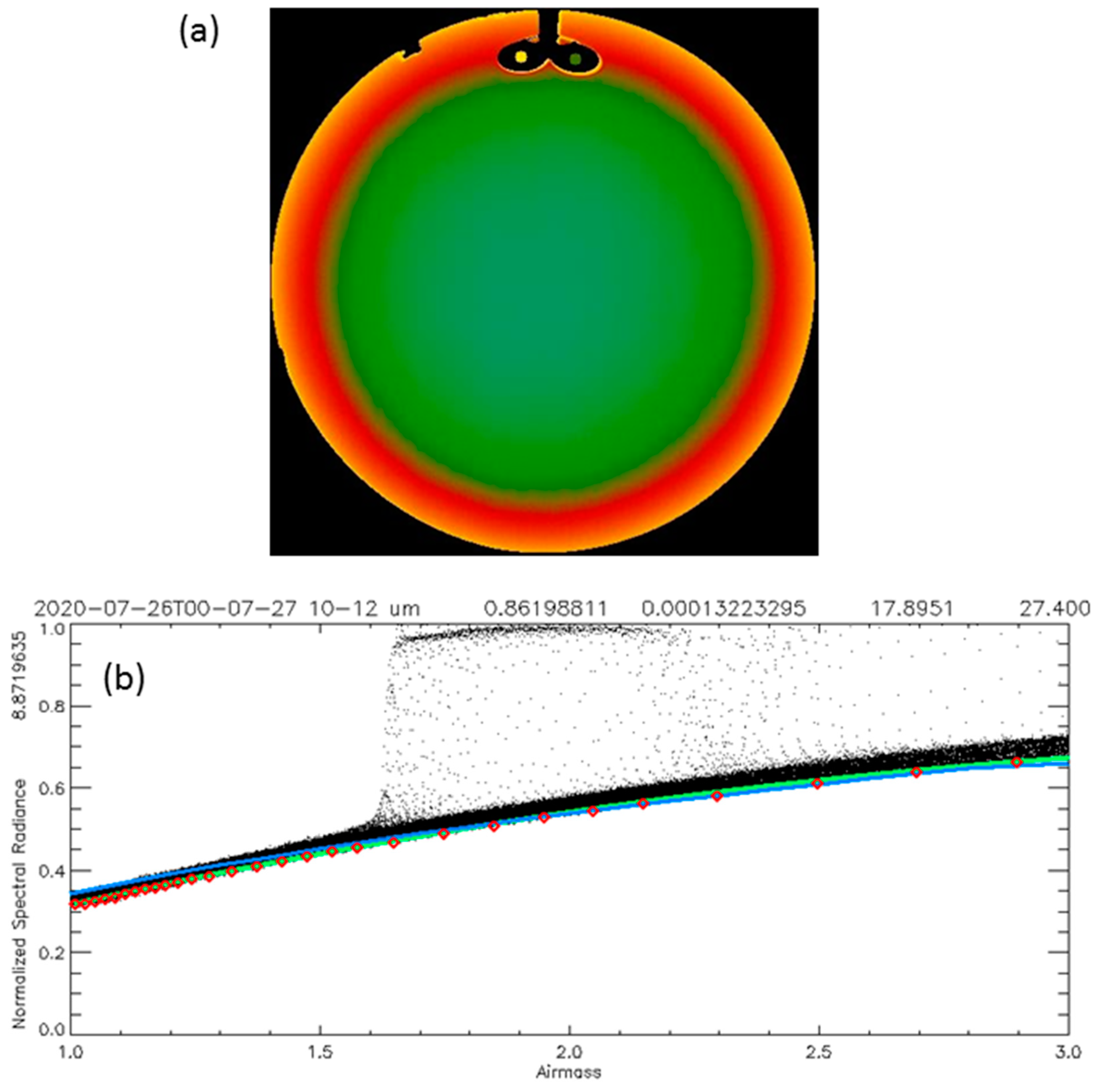
The sensor we used is the ASIS1i imager developed by SOLMIRUS (Colorado Springs, Colorado, USA). It is an IR-only version of a larger model of ASIVA imager that additionally includes a visible sensor (see references [15,16,17]). The whole sky cloud sensor is geo-located and can continuously (and at a relatively high rate) measure and retrieve whole sky parameters in 0.5° spatial resolution and geo-location accuracy of 0.25° per pixel. The ASIS1i sensor integrates an uncooled IR camera (calibrated by a built-in black body) and operating software (Figure 5). An embedded filter wheel with carefully selected filters enables multispectral data collection that improves the quality of the retrieved sky parameters. Cloud detection and optical depth are carried out by comparing the down-welling radiance from each point in the sky to a careful estimation of clear sky radiance. It is accomplished by two methods, each of them optimal at different cloud covers. At relatively low cloud-cover, (less than about 50%) there are enough clear sky patches in the whole sky image, and the clear sky radiance estimation can be retrieved directly from a scattergram plot of the downwelling radiance at every elevation angle. At high cloud-cover, the cloud sky radiance is estimated by running the MODTRAN [18] model with temperature (T) and relative humidity (RH) vertical profiles assessed in two possible ways (one based on near-surface T and RH sensor readings, the other on modified MLS (Mid Latitude Summer) built-in MODTRAN model).
Note in Figure 5 the azimuthal symmetry of the brightness temperature of the sky which is the key factor for a clear sky radiance estimation. The clear sky brightness temperature strongly depends on the elevation angle, especially at low altitudes. At any point in the sky, any deviation from the clear sky brightness temperature is always upwards and can be attributed to the presence of a cloud. The brightness temperature of the cloud is a function of its liquid water content (LWC), integrated water content (IWC), type, base height, and elevation angle. It can never exceed the air temperature near the ground. The sensor provides the following products in FITS (Flexible Image Transport System) format for each spectral band:
- Normalized temperature image—obtained by division of the effective temperature in each pixel within the field of view (FOV) by the closed sensor cover (hatch) temperature and additional correction by the two black bodies in the FOV in which their temperatures are measured continuously. The obtained valid values range between 0 to 1 (except for the sun and the moon).
- Brightness temperature images of the whole sky. These values are always smaller than the corresponding air temperatures. So far at our location, the minimal zenith brightness temperature we measured was 198 K. These images are also available in processed jpeg format for quick visualization and qualitative analysis.
- Clear sky subtracted image. Each pixel has a value that reflects its difference from the clear sky estimation. We used as thresholds the following values: under 0.05—clear sky, 0.05–0.1—thin clouds, above 0.1—thick clouds.
- Total thick and thin cloud sky cover for each whole sky image, which is the fraction of the sky hemisphere that is covered by this cloud type. It is calculated according to the following formulation:
We extracted from these products the following parameters for our analysis of the fog event:
Whole sky brightness temperature map: We expect to get a typical clear (or partially cloudy) sky image when fog is absent (Figure 5b), and a uniform brightness temperature sky image equal to air temperature when fog is present.
From the clear sky subtracted images, the total cloud coverage of the sky of thin and thick clouds (or fog in our case) is calculated according to the preset thresholds (see Equation (3)).
We will show in our analysis that these two products provide useful information to study the fog formation and dissipation processes.
2.2.2. Doppler Wind Lidar
Pulsed Doppler Lidar is a remote sensing technology used to measure the atmospheric vertical profile of winds and aerosol load. Atmospheric aerosols and clouds backscatter the transmitted pulses of near-infrared radiation, and the obtained Doppler shift impact on the backscattered light is proportional to the line-of-sight component of the scatterers’ velocity. The strength of the aerosol return signal depends upon the amount of aerosol in the atmosphere [19]. Since the signal retrieved from a pulsed Doppler Lidar under fog conditions depends on the backscatter and extinction coefficients of its droplets, it is a highly effective research tool for fog characterizations. The Doppler Lidar performed measurements in “stare” mode, in which the Lidar “stared” at a fixed elevation angle of 90 degrees.
For a transmitted rectangular monostatic single-wavelength pulsed Lidar with instantaneous power Po, the received power, Ps, at range R due to aerosol backscatter, is given by the common form of the single scattering Lidar equation:
where c is the speed of light and τ is the pulse duration. Arec is the effective receiver area, Arec/R2 is the solid angle [sr] subtended by the receiver. ηSYS is the system’s optical efficiency and O(R) is the range-dependent overlap function, which approaches unity after a relatively short distance.
The Lidar equation (Equation (4)) usually cannot be solved explicitly since it is a single equation with two unknowns, σext and β. Often in the field of atmospheric measurements, prior assumptions of Klett [20] are made about the cloud type with an assumed relationship between σext and β. The formulation is often used to retrieve the optical parameters of the profile from the Lidar data, by estimating the Lidar equation initial value.
However, in the current setup, the simultaneous in situ measurements of droplets-size distribution allows a direct calculation of the time-dependent parameters of the Lidar equation, σext and β, and to fully solve it without the aforementioned assumptions. In Section 3.2 we will show that the Ps vertical profile calculated using the Lidar equation (Equation (4)) agrees with the Lidar measured signal and describes well the evolution in time of the fog.
3. Results: Meteorological Parameters and Their Reflection on the Remotely Sensed Products
In this section, we present the measured findings showing the temporal variability of the various parameters describing the January 2021 fog event. First, we show the fog behavior as reflected in the sky imager IR sensor and then we analyze the measurements by the Doppler Lidar.
3.1. WSI
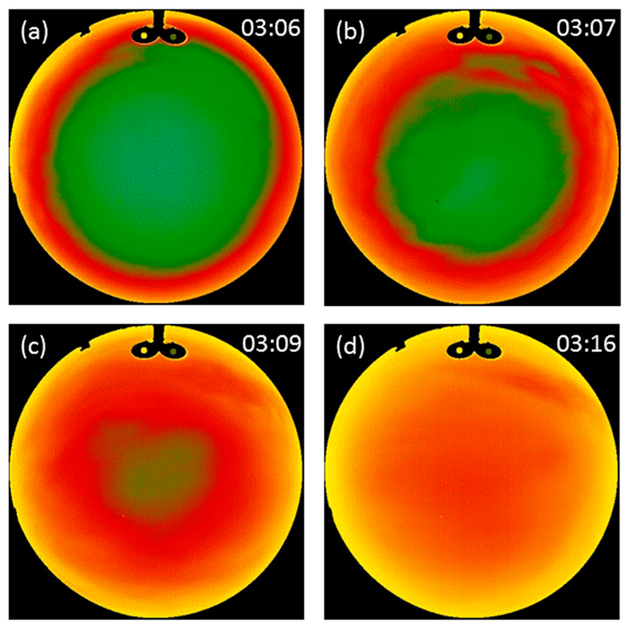
We used the following simple technique to illustrate in a tangible way the evolution of fog with time, as seen in Figure 6, Figure 7 and Figure 8. The time stamps in all of the panels are given in Israel Local Time (LT = UTC + 2). Sunrise took place at 06:42 LT. Figure 6 follows the fog formation on 4 January 2021.
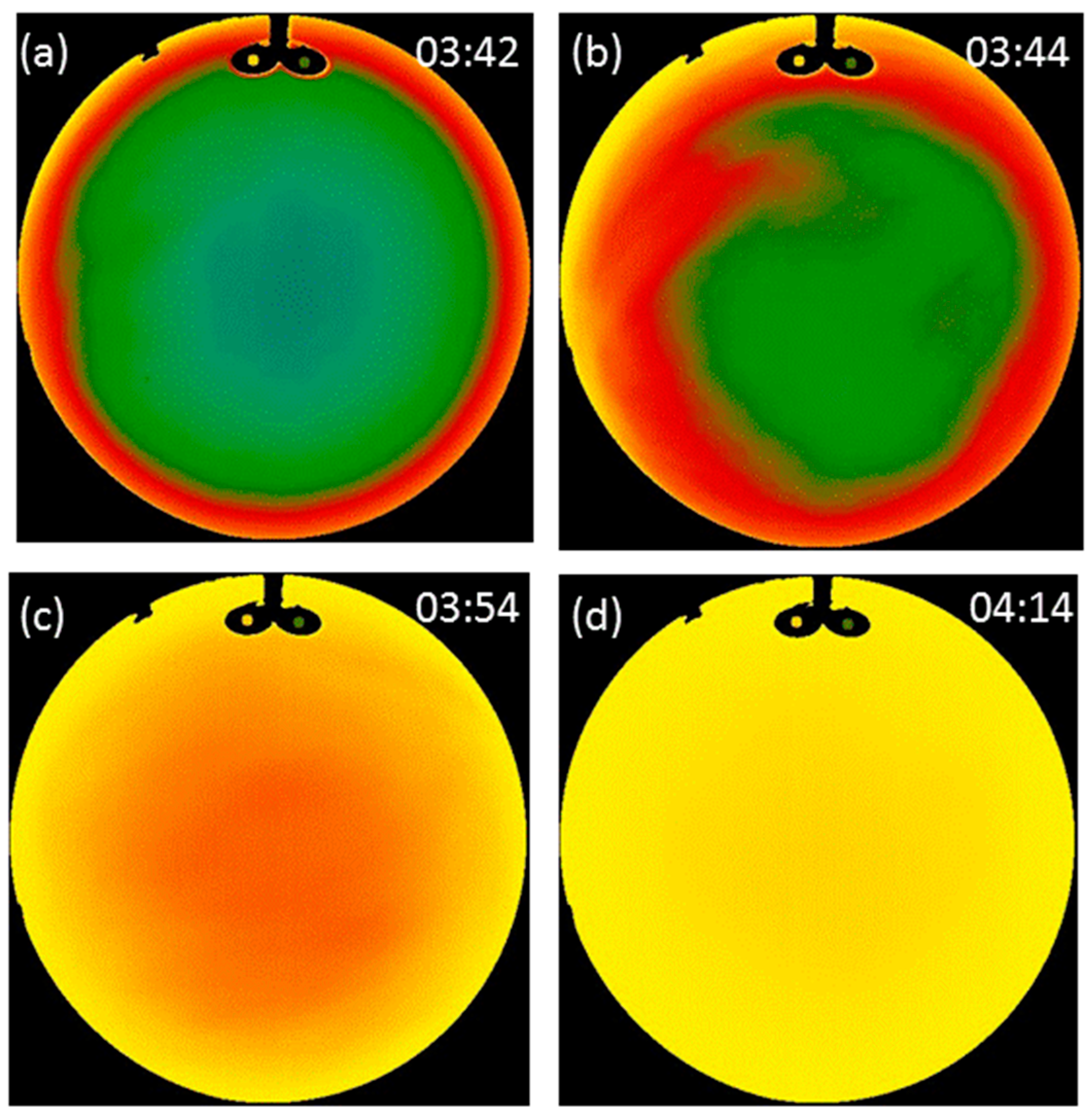
Figure 6 shows the fast and symmetrical development of the fog event within the field of view of the WSI. The images suggest that fog was neither advected nor gradually filling the field of view from one specific direction. The images reveal that the fog developed locally and continuously within the field of view, growing vertically above the ground. This is clearly seen in the fisheye lens images, where constant elevation angle is expressed in the form of circles of the same brightness temperature. Since the brightness temperature of the sky during the formation of the fog did not break this symmetry, there was no other direction of movement in the field of view. The fog that formed on 6 January 2021 presents a similar behavior, as shown in Figure 7.
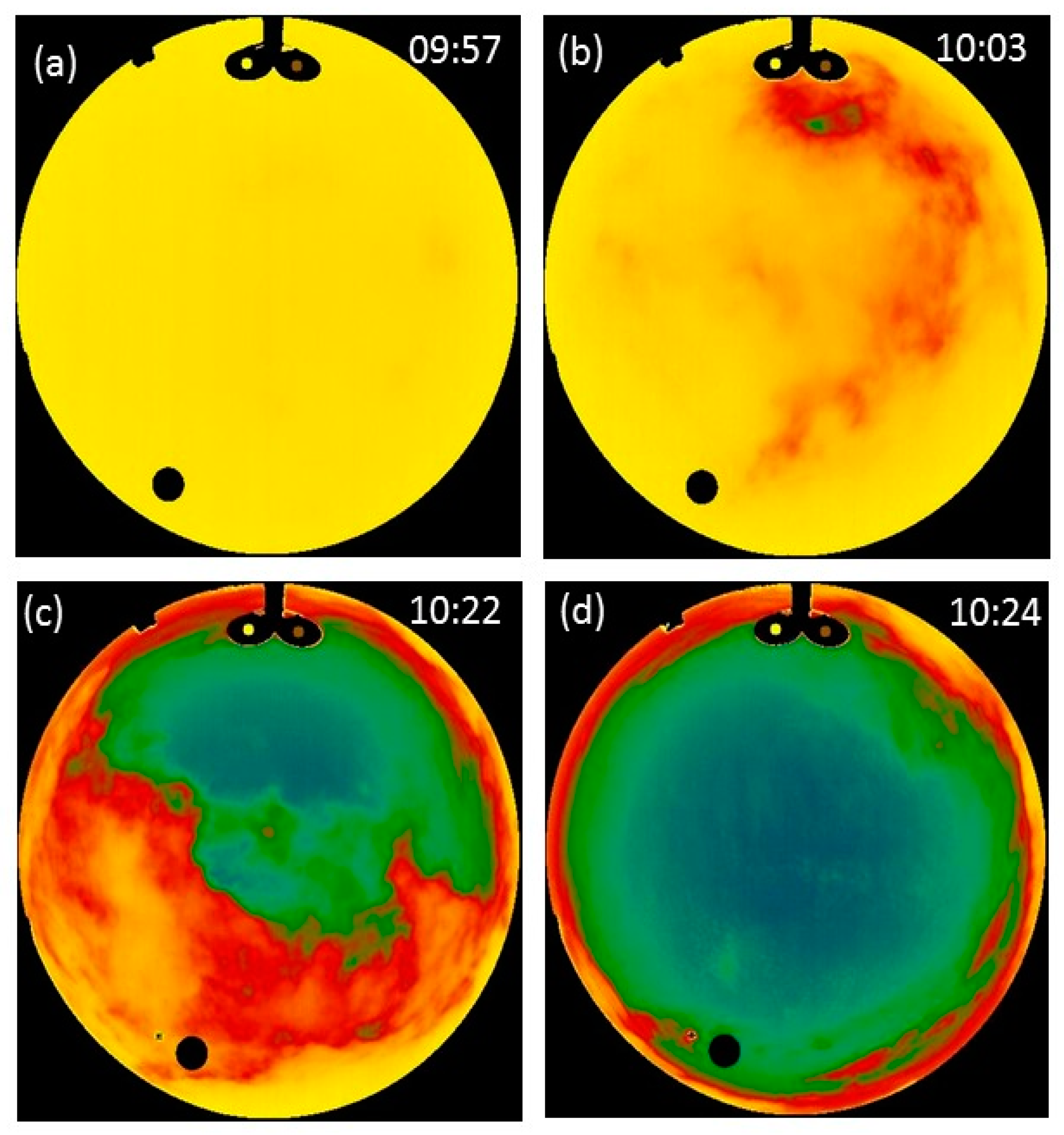
Fog clearing on 6 January 2021 is shown in Figure 8.
Figure 6, Figure 7 and Figure 8 demonstrate that useful and meaningful information can be retrieved from IR WSI to study fog formation and dissipation. IR imaging is effective at night and at low light level conditions where visible cloud sensors are ineffective. Furthermore, the combination of the whole sky view and the interpretation of the brightness temperature can add valuable information such as: is the fog formed on-site or advected? How fast did it develop and dissipate? How dense is it? (The last question can be interpreted through the value of the zenith brightness temperature, see Appendix A).
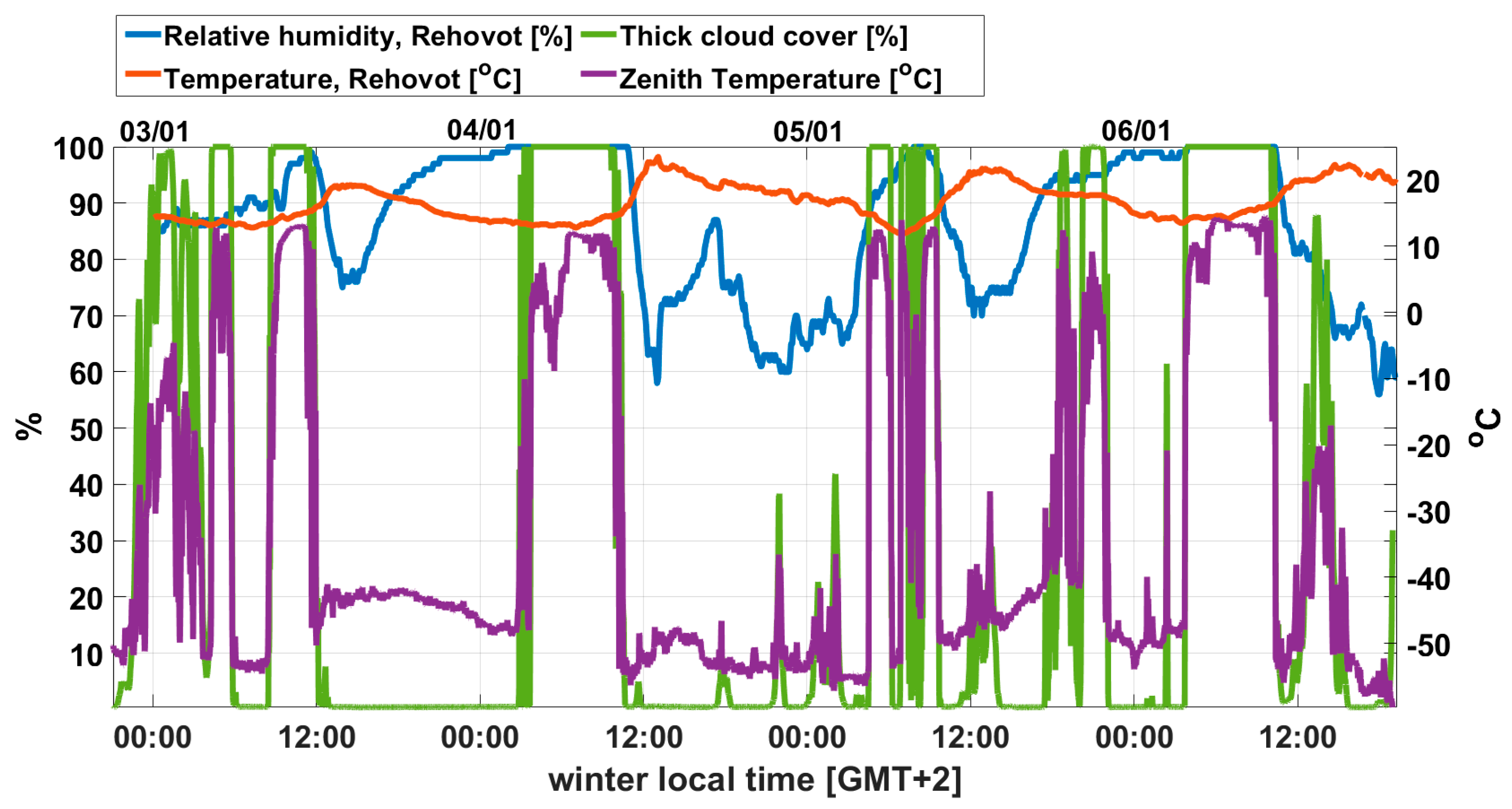
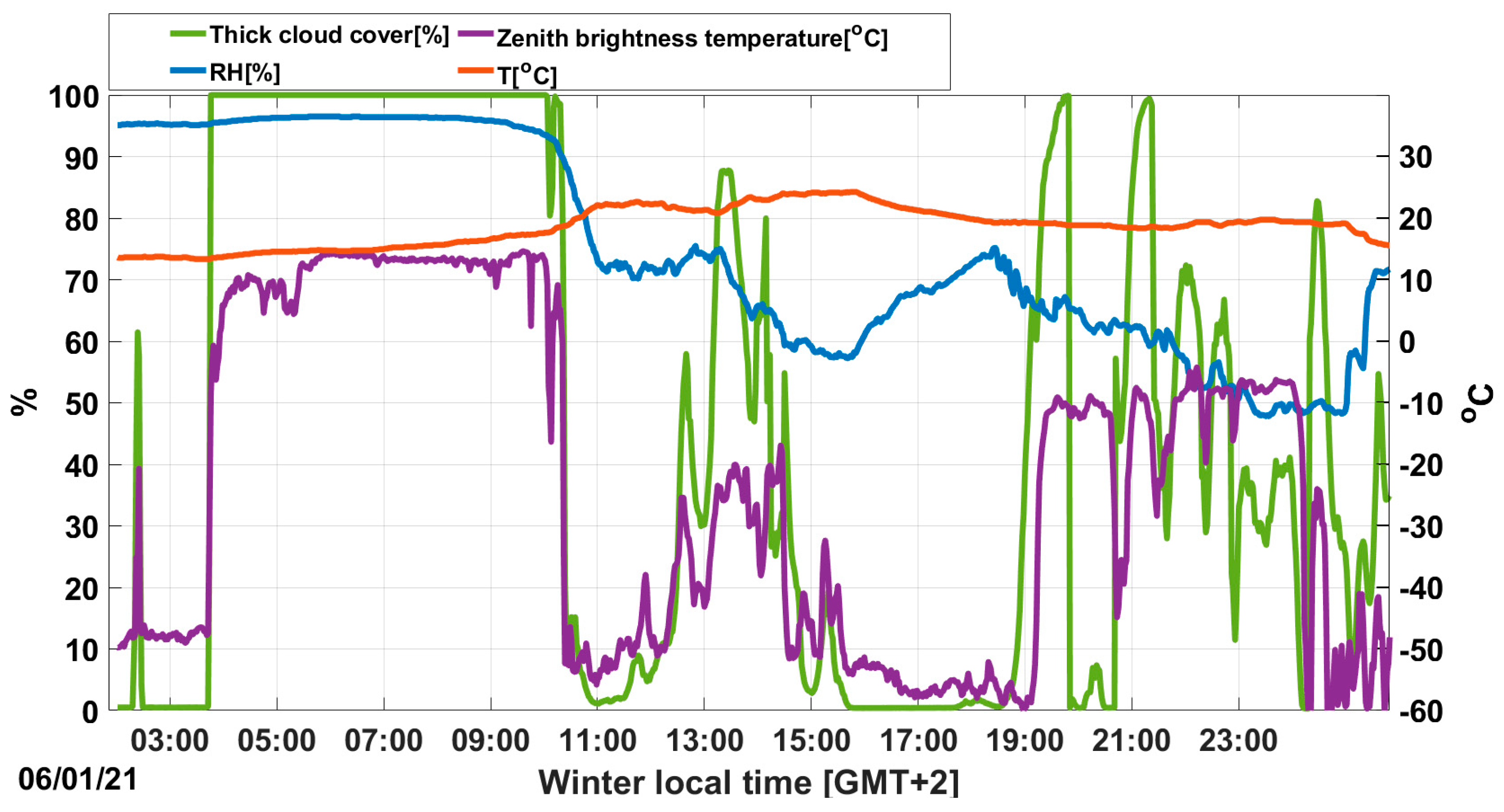
The meteorological properties of the fog event, along with the zenith brightness temperature and the cloud cover of thick clouds obtained from the WSI sensor, are shown in Figure 9.
It can be seen in Figure 9, that during the four nights, the fog started after midnight and dissipated by the late morning. The zenith brightness temperature and the cloud cover percentage values show a step-like shape, unlike “conventional” low clouds. Cloud fields are characterized by a dynamic sky coverage that results in a much more round and irregular shape (see more rigorous data analysis in Section 3.1.1). Since the fog layer is thick, the zenith temperature is very close to the air temperature. This is also a unique feature of fog events, which by definition occur at surface level, as opposed to cloudy skies at higher altitudes (and therefore in much colder environments). The difference between the zenith brightness temperature and the surface air temperature is a strong indication of the fog layer density and height (see appendix), clearly seen in the long-lived 4 January and 6 January fog events.
To conclude this chapter, radiation fog that is observed in SWI is characterized by three main properties:
1. Azimuthal symmetrical shape during the buildup phase. Higher sky brightness temperatures emerge in a radial symmetry from low elevation angles towards the higher ones.
2. The obtained zenith brightness temperature is very close to air temperature.
3. Sharp rise (such as a step function) from zero, or very little cloud cover, to completely cover cast sky. In the following subsections we will show that, unlike radiation fog, cloudy skies (and we assume also that advection fog) have different characterizations.
3.1.1. Comparison of the Buildup and Dissipation of a Cloudy and Foggy Sky with WSI
This subsection provides additional support, both qualitative and quantitative, for the conclusions about the unique characterization of the formation and dissipation of fog as opposed to overcast cloud cover. The remarkable difference between cloudy sky and heavy cloudiness in the WSI can be found even within the fog event itself.
As seen in Figure 10, the fog event was followed by the passage of two low cloud fields within the FOV of the WSI. These fields are characterized as expected by gradual buildup and dissipation and frequent changes in cloud cover due to the specific cloudiness properties over our measurement site. Thin cloud classification at cloud edges is also present.
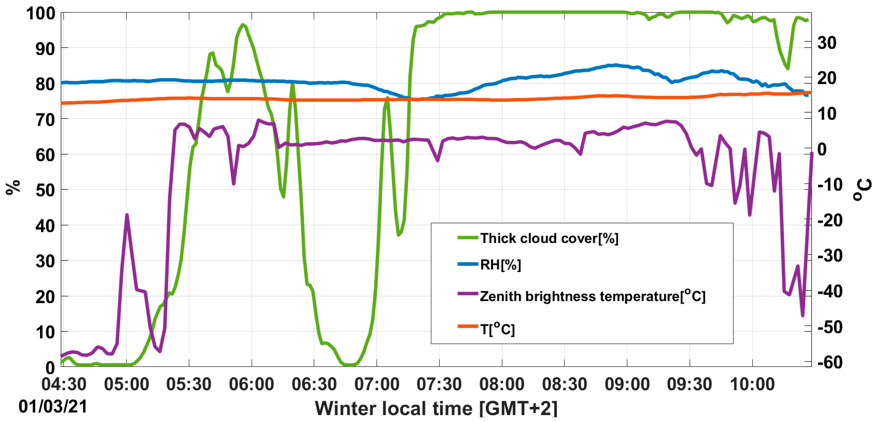
The observed zenith brightness temperature during passing cloud fields is much lower than the air temperature. It corresponds to the air temperature at cloud base height, modified by the atmospheric transmission and path radiance. It always yields a slightly higher apparent temperature of the cloud base relative to the actual one. The temperatures of the air layers below the cloud base are usually higher than that of the cloud base layer. The emissivity of a thick water droplets cloud is close to unity in the Long Wave IR band [21]. An example of an analysis of a totally overcast sky is shown in Figure 11 and Figure 12.
This case study nicely demonstrates the difference between the evolution and the appearance of foggy and cloudy skies. First, fully overcast skies evolve on significantly longer time scales relative to fog (tens instead of a few minutes). As in any typical cloud field, the cloud cover builds up gradually in time with the local geometry playing an appreciable role in its appearance. During the buildup phase, the cloud cover may change its pace and can even temporally retreat. In addition, during this phase, low emissivity clouds are also present in the field of view. Second, from the ground level field of view, most clouds are advected at the wind speed observed at their base height. Therefore, clouds begin to accumulate in the field of view from a specific direction. The azimuthal symmetry of the fog formation in the field of view (see Figure 6) is a unique feature of a radiation fog event as it does not evolve from a preferred direction. Third, the zenith brightness temperature of clouds never reaches the observed values of air temperature in the ground level as in a foggy sky. As noted in Section 3.1, the apparent temperature of a cloud is derived from the cloud base temperature that depends on the air temperature at the same height. This temperature is always significantly lower than the air temperature near the ground (see Appendix A).
3.1.2. Comparison of Radiative and Convective Fog Seen on WSI
We should be somewhat cautious about the conclusions regarding the characterization of fog with WSI since they refer to radiation fog only. Advection fog, as its terminology suggests, is advected from a preferred direction and hence the image of its buildup in the WSI FOV cannot be symmetrical as shown in Figure 6. It is also important to observe that the image of advection fog cannot be distinguished from the case when low clouds completely cover the ground level in mountainous areas. However, the distinctive feature of the radiative temperature of fog remains for advection fog, since the zenith brightness temperature corresponds to ground level air temperature. Thus, in low elevation and flat terrain, high zenith temperatures can be attributed only to fog events.
3.2. StreamLine Doppler Lidar
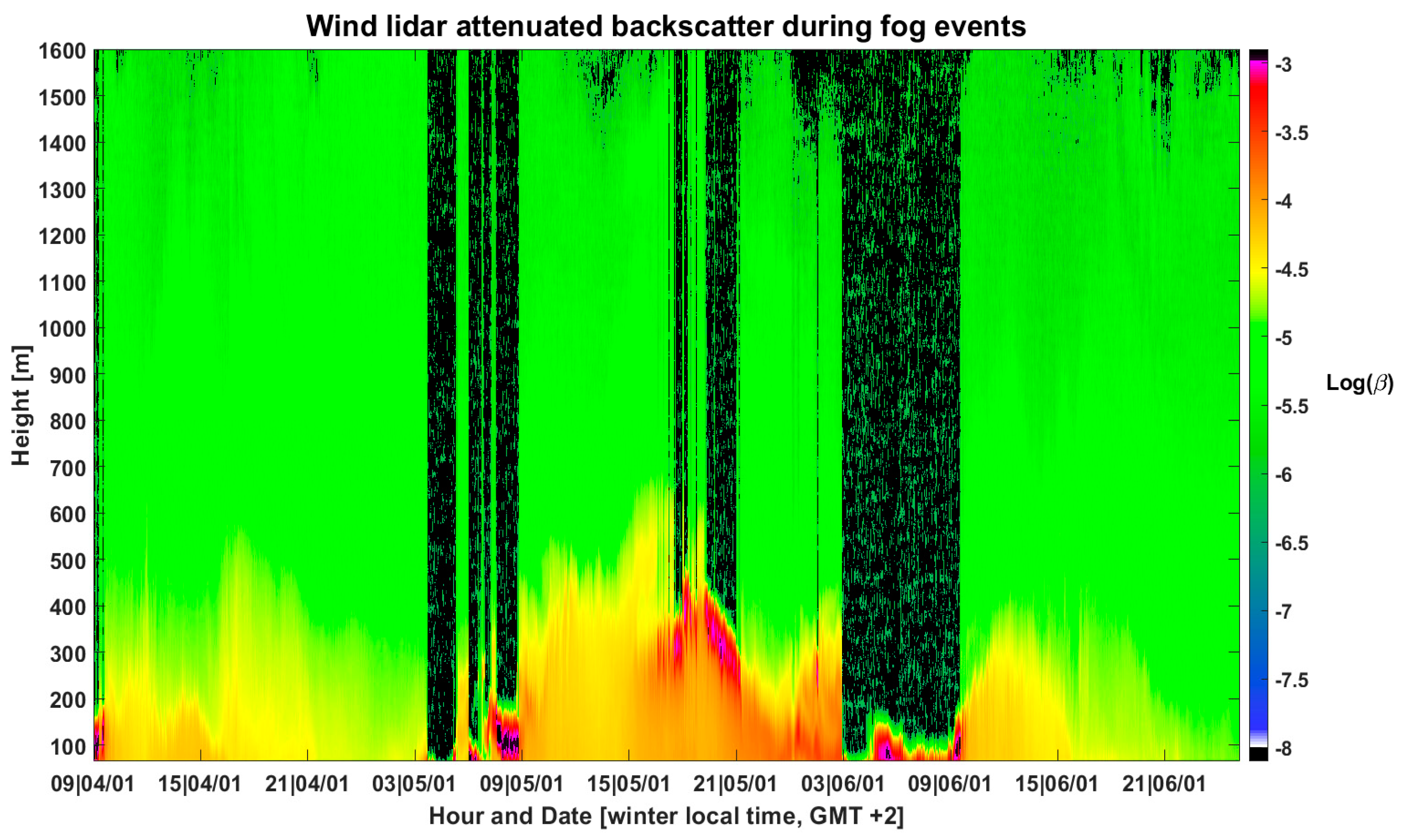
The Halo-Photonics Doppler Lidar was operated in a vertically staring mode during the entire fog events. Its spatial resolution is 1.5 m, and the time resolution was 1 s in this specific set-up. The measured backscattered signal of the fog events of 4 January 2021–6 January 2021 is presented in Figure 13, showing clearly the reduction in the signal due to fog during the early morning hours (~3:40–10:00 a.m. on 5 January 2021 and 6 January 2021).
In order to examine the measured Lidar output, the theoretical Lidar attenuated backscatter, Ps, was calculated using the Lidar equation (Equation (4)), based on the droplet-size measurements.
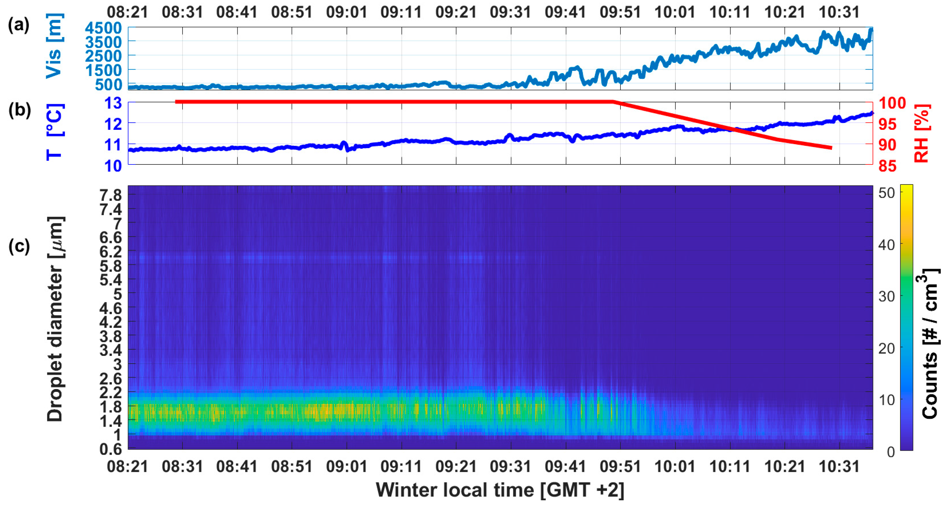
Figure 14 presents the fog typical conditions during our measurements: visibility, temperature, relative humidity, and droplets-size distribution. It can be seen that the January fog is characterized by a minimum visibility range of 90 m and the droplets-size main mode of droplets diameter between 1 to 2 µm, followed by another mode around 6 µm. No droplets were larger than 8 µm. Fog dissipation is shown clearly at 09:50 LT, followed by a decrease in the relative humidity, increase in the visibility range and disappearance of larger droplets.
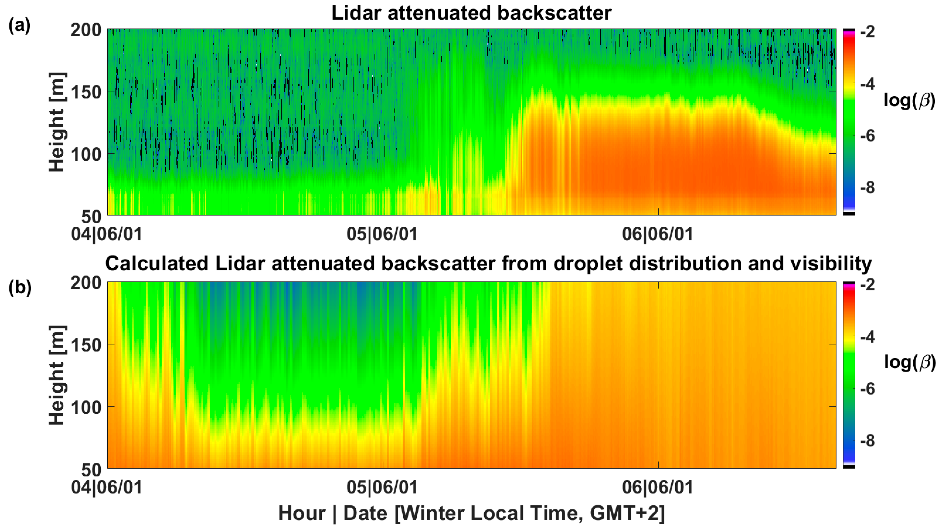
The calculation of Ps following the Lidar equation (Equation (4)) is now possible. σext and β are derived based on the measured ground droplets-size distribution shown in Figure 14b, and assuming, for simplicity, that all constants in Equation (4), equal unity. The result of their use in the Lidar equation, Equation (4), is shown in Figure 15b, in comparison to the attenuated backscatter measured by the Doppler Lidar (Figure 15a).
It can be seen that a reasonable agreement is achieved between the theoretical and measured attenuated backscatter Lidar signal. The main limitation of this derivation is the assumption of a homogeneous fog layer with a roughly estimated depth. As can be seen, the vertical extent of the heights in Figure 13 is up to only 200 m based on our assumption based on the Tel-Aviv photograph (Figure 1). The difference between the theoretical and measured profile at its upper part arises from the inhomogeneity of the fog that seems to dissipate at those heights, in contrast to the calculated signal that assumes homogeneous fog concentration along with the profile height. Therefore, the above use of the Lidar equation is limited to cases where ground measurements of the droplets size distributions are available. Additionally, homogeneity of the fog layer, a property that depends on fog type, should be assumed.
4. Discussion and Summary
Using as a case study a dense regional-scale radiation fog event, we showed the usefulness of multi remote sensing measurements in the analysis and characterization of fog. The combination of the remotely sensed data with surface-level measurements provides interesting and unique insights about the fog properties, including its time evolution, depth and duration. The synergy between different sensors enriches the acquired data and its interpretation. It should be observed, however, that this study is based on a one-time radiation fog event and therefore further analysis regarding future events is required. We showed that useful information is retrieved from an IR WSI which enabled us to study the fog formation and dissipation. It showed that the fog developed locally as opposed to being advected and thus provided information about the temporal evolution of the formation, life, and dissipation of the fog. The combination of the whole sky viewer and the analysis of the brightness temperature adds valuable information to describe the fog properties. A heavy and dense surface-level fog layer leads to homogenous brightness temperature for the whole sky image, which has the same value of air temperature at surface level. Otherwise, patches of lower brightness temperature in the sky hemisphere are observed. A thin layer of fog can be also manifested through angular dependence of the brightness temperature of the sky due to partial transparency of the fog layer against the cold clear sky background.
The course of the zenith brightness temperature and effective cloud cover during a fog event is very different from that characterizing the formation of a fully overcast low-altitude cloud cover. Therefore, WSI data can be used to differentiate between these two states. It enhances the usefulness of all-sky images and closes the gap between clouds and fog in the data interpretation.
The use of a Doppler Lidar as a sensor for investigating fog events proves useful, due to its signal reduction under fog conditions. The good agreement between the theoretical attenuated backscatter profile that was achieved by measuring the droplets size distribution with the measured profile, validated the use of a Doppler Lidar as a monitoring tool for fog events, possible for continuous measurements of fog in fixed locations. A different location may involve other types of fog and will require additional validation measurements to define the fog properties.
It was shown that fog can be monitored by these two stand-off-sensing technologies that were not originally designed for such a capability, almost without additional observations. It enables the monitoring of fog properties based only on remote sensing, without the need for a dedicated field campaign. We believe that our work is a pioneering endeavor that encompasses simultaneous remote sensing measurements and analysis of a fog event with a thermal IR WSI. Useful and meaningful information can be retrieved from this instrument to study fog formation and dissipation. Therefore, we conclude that incorporating these sensors for fog research, either as a part of wider measurements deployments or as stand-alone instruments, can enhance our knowledge and understanding of the complex variety of fog events.
Author Contributions
A.R., E.A. and T.T. designed and performed the experiments and analyzed the data. A.R. and E.A. contributed analysis tools and materials. A.R., E.A. and D.R.-E. wrote the paper. All authors have read and agreed to the published version of the manuscript.
Funding
This research received no external funding.
Institutional Review Board Statement
Not applicable.
Informed Consent Statement
Not applicable.
Data Availability Statement
Not applicable.
Acknowledgments
The authors would like to thank Yehuda Alexander for his review and helpful comments.
Conflicts of Interest
The authors declare no conflict of interest.
Appendix A. Radiative Transfer Equation of Cloud Observation in the LWIR
As described in Section 3.1, due to the azimuthal symmetry of the sky radiance, and as long as the cloud base height is kept constant, the observed radiance in the Long Wave InfraRed (LWIR) band is a function of elevation angle only. The general radiative transfer equation for a cloud observation in the LWIR band is given by:
where is the path radiance from the ground to the cloud base height and is a function of the T and RH profiles, and is the atmospheric transmission between the ground and the cloud base height. is the cloud emission, which is a function of cloud emissivity and its temperature, and is the path radiance from the cloud ceiling to TOA (top of the atmosphere).
For all cloud types, except high altitude cirrus, for cloud thickness more than a few tens of meters, and can be estimated as a black body radiator with a temperature of the air at the cloud base height, . B(T) denotes the black body radiation at a temperature T in the LWIR band. The last term of Equation (A1) is the path radiance from the cloud ceiling to TOA and is zero for thick clouds.
When we consider a thick fog event, the cloud base height is at ground level, and the first term in Equation (A1) vanishes. Therefore, . Note that since there is no path radiance, the dependence on the elevation angle is lost and . Moreover, a fog event characterized by , is not dense enough to produce emissivity of unity, and the third term in Equation (A1) becomes significant.
For a low thick cloud layer, . Since is always less than Tair, then . Additionally, since the first term of Equation (A1) does not vanish for a cloud, the elevation dependence is slightly retained.
References
- World Meteorological Organization: Fog. Available online: https://www.wmocloudatlas.org/fog.html#sthash.11lruLve.dpuf (accessed on 25 April 2021).
- Goldreich, Y. The Climate of Israel: Observation, Research and Application; Springer Science & Business Media: Berlin, Germany, 2012; p. 129. [Google Scholar]
- Levi, W.M. Fog in Israel. Isr. J. Earth Sci. 1967, 16, 7–21. [Google Scholar]
- Alpert, P.; Osetinsky, I.; Ziv, B.; Shafir, H. Semi-objective classification for daily synoptic systems: Application to the Eastern Mediterranean climate change. Int. J. Climatol. 2004, 24, 1001–1011. [Google Scholar] [CrossRef]
- Special Review of the Rare Fog Event Published by The Israel Meteorological Service (IMS). Available online: https://ims.gov.il/sites/default/files/2021-01/%D7%A8%D7%A6%D7%A3%20%D7%99%D7%9E%D7%99%20%D7%A2%D7%A8%D7%A4%D7%9C%20%D7%99%D7%A0%D7%95%D7%90%D7%A8%202021.pdf (accessed on 28 April 2021). (In Hebrew)
- Heavy Fog in the Morning. Available online: https://www.ynet.co.il/news/article/r1LLtT0Tv (accessed on 3 January 2021).
- Cloud Observations with Sky InSight™ All-Sky Imager. Available online: https://reuniwatt.com/en/247-all-sky-observation-sky-insight (accessed on 21 August 2021).
- Rösner, B.; Egli, S.; Thies, B.; Beyer, T.; Callies, D.; Pauscher, L.; Bendix, J. Fog and Low Stratus Obstruction of Wind Lidar Observations in Germany—A Remote Sensing-Based Data Set for Wind Energy Planning. Energies 2020, 13, 3859. [Google Scholar] [CrossRef]
- Gultepe, I.; Fernando, H.J.S.; Pardyjak, E.R.; Hoch, S.W.; Silver, Z.; Creegan, E.; Leo, L.S.; Pu, Z.; De Wekker, S.F.J.; Hang, C. An overview of the MATERHORN fog project: Observations and predictability. Pure Appl. Geophys. 2016, 173, 2983–3010. [Google Scholar] [CrossRef]
- Bohren, F.; Huffman, D.R. Absorption and scattering by a sphere. In Absorption and Scattering of Light by Small Particles; Wiley: New York, NY, USA, 1998; Chapter 4; pp. 82–129. [Google Scholar]
- Mätzler, C. MATLAB Functions for Mie Scattering and Absorption, v.2. IAP Res., Bern, Schweiz, Rep. 8 no. 1, Jun. 2002. Available online: https://omlc.org/software/mie/maetzlermie/Maetzler2002.pdf (accessed on 1 February 2021).
- D’Almeida, G.A.; Koepke, P.; Shettle, E.P. A Global Aerosol model. In Atmospheric Aerosols: Global Climatology and Radiative Characteristics; A Deepak Pub: Hampton, VA, USA, 1991; Chapter 4, Section 4.5; pp. 56–60. [Google Scholar]
- Available online: https://meteo.moag.gov.il/home/map? TargetIds = 11 (accessed on 10 January 2021).
- Available online: https://ims.data.gov.il (accessed on 10 January 2021).
- Shaw, J.A.; Nugent, P.; Pust, N.J.; Thurairajah, B.; Mizutani, K. Radiometric cloud imaging with an uncooled microbolometer thermal infrared camera. Opt. Express 2005, 13, 5807–5817. [Google Scholar] [CrossRef] [PubMed]
- Sebag, J.; Andrewa, J.; Klebe, D.; Blatherwick, R.D. LSST All-Sky IR Camera Cloud Monitoring Test Results. In Proceedings of the SPIE 7733, Groundbased and Airborne Telescopes III, San Diego, CA, USA, 5–6 August 2010; Volume 773348. [Google Scholar]
- Klebe, D.; Blatherwick, R.D.; Morris, V.R. Ground-based All-Sky Mid-Infrared and Visible Imagery for Purposes of Characterizing Cloud Properties. Atmos. Meas. Tech. 2014, 7, 637–645. [Google Scholar] [CrossRef] [Green Version]
- Berk, A.; Conforti, P.; Kennett, R.; Perkins, T.; Hawes, F.; van den Bosch, J. MODTRAN6: A major upgrade of the MODTRAN radiative transfer code. In Proceedings of the SPIE 9088, Algorithms and Technologies for Multispectral, Hyperspectral, and Ultraspectral Imagery XX, 90880H, Baltimore, MD, USA, 5–9 May 2014. [Google Scholar] [CrossRef]
- Pearson, G.; Davies, F.; Collier, C. An analysis of the performance of the UFAM pulsed Doppler lidar for observing the boundary layer. J. Atmos. Ocean. Technol. 2009, 26, 240–250. [Google Scholar] [CrossRef]
- Klett, J.D. Stable analytical inversion solution for processing lidar returns. Appl. Opt. 1981, 20, 211–220. [Google Scholar] [CrossRef] [PubMed] [Green Version]
- Shaw, J.A.; Nugent, P.W. Physics principles in radiometric infrared imaging of clouds in the atmosphere. Eur. J. Phys. 2013, 34, S111–S121. [Google Scholar] [CrossRef]
Figure 1.
Heavy fog covers Tel-Aviv buildings, 3 January 2021, during early morning hours [6].
Figure 1.
Heavy fog covers Tel-Aviv buildings, 3 January 2021, during early morning hours [6].

Figure 2.
(a) IMS Radiosonde measurement before and during fog periods, from left to right: Horizontal wind speed and direction, air and dew point temperatures, mixing ratio and relative humidity. (b) Visibility values in Ness Ziona before and during the fog event.
Figure 2.
(a) IMS Radiosonde measurement before and during fog periods, from left to right: Horizontal wind speed and direction, air and dew point temperatures, mixing ratio and relative humidity. (b) Visibility values in Ness Ziona before and during the fog event.

Figure 3.
Field-experiment area map [Google] showing the measurement site in Ness Ziona and the meteorological stations nearby.
Figure 3.
Field-experiment area map [Google] showing the measurement site in Ness Ziona and the meteorological stations nearby.

Figure 4.
Field-experiment instrumentation: (a) Sky imager [ASIS1i, SOLOMIRUS, Colorado Springs, CO, USA]. (b) Droplet-sizes measurements [FSSP-100, PMS, Boulder, Colorado, USA]. (c) Visibility-range sensor [SWS250, Biral, Bristol, UK]. (d) Doppler Lidar [StreamLine XR, Halo photonics, Leigh, UK].
Figure 4.
Field-experiment instrumentation: (a) Sky imager [ASIS1i, SOLOMIRUS, Colorado Springs, CO, USA]. (b) Droplet-sizes measurements [FSSP-100, PMS, Boulder, Colorado, USA]. (c) Visibility-range sensor [SWS250, Biral, Bristol, UK]. (d) Doppler Lidar [StreamLine XR, Halo photonics, Leigh, UK].

Figure 5.
An example of JPEG qualitative images that are produced by the sensor for a quick look at the sky conditions. (a) An image of a midsummer clear sky from 26 July 2020 in a color scale of the brightness temperature. The scale runs from yellow-orange-red-green-blue from high to low temperatures respectively. The full-color scale in this image corresponds to a brightness temperatures span of about 230–300 K (red is hot). The non-valid pixels appear in black. The calibration mast with two blackbodies is visually observed on the top of the image. (b) A visual graph of the corresponding scatter plot of the brightness temperature (expressed as normalized radiance with respect to ground level temperature) as a function of air mass is used for clear sky estimation. The three-color lines correspond to the different clear sky radiance estimation methods which typically overlap each other at clear sky conditions. It should be noted that these images do not hold quantitative data, and are used only for basic interpretation and for the analysis of the spatial and temporal evolution of the cloud and fog field. The quantitative data were used for obtaining the results depicted in Figures 9–11.

Figure 6.
Sky image at 4 January 2021. (a) 03:06—the fog is low and the whole sky image is clear. (b) 03:07—the fog is rising rapidly as indicated by the increased brightness temperature of the sky at low elevation angles. (c) 03:09—the fog continues to rise, but the clear sky is still present near the zenith. (d) 03:16—the fog covers the entire sensor’s field of view, but not very densely, as the sky image is not completely homogenous.

Figure 7.
Sky image on 6 January 2021. (a) 03:42—the fog is low and the sky image is clear. (b) 03:44—the fog is rising rapidly. The slight asymmetry shows that the fog developed from the northeast direction. (c) 03:54—the fog covers the entire sensor’s field of view, but not very densely. There is still a temperature gradient that follows the elevation angle. (d) 04:14—Fully developed dense fog. The sky brightness temperature is homogenous and its magnitude is the same as the air temperature.

Figure 8.
Sky image on 6 January 2021. (a) 09:57—Fully developed dense fog. (b) 10:03—the fog begins to dissipate. Low-density patches are clearly visible. (c) 10:22—Snapshot in the middle of the rapid clearing process. Half of the sky is clear. (d) 10:24—the sky is almost completely clear. Some residual fog patches are still present close to the ground.

Figure 9.
Relative humidity and air temperature along with the zenith temperature and thick cloud cover, during the January 2021 event, taken from “Rehovot” station. The X-axis time label denotes time- noon or midnight/date between 3–7 January 2021.
Figure 9.
Relative humidity and air temperature along with the zenith temperature and thick cloud cover, during the January 2021 event, taken from “Rehovot” station. The X-axis time label denotes time- noon or midnight/date between 3–7 January 2021.

Figure 10.
Cloud cover and zenith brightness temperature report during the fog event of 6 January 2021, calculated from WSI data. Note that the relative humidity and the air temperature are taken directly from the sensors embedded in Asis1i. Therefore, their values represent much more accurately the true values near the sensor. However, the humidity sensor cannot measure RH above 97.8% (compared to Figure 9).

Figure 11.
Cloud cover and zenith brightness temperature report during 1 March 2021, calculated from WSI data. The relative humidity and the air temperature are obtained from the sensors embedded in Asis1i.
Figure 11.
Cloud cover and zenith brightness temperature report during 1 March 2021, calculated from WSI data. The relative humidity and the air temperature are obtained from the sensors embedded in Asis1i.

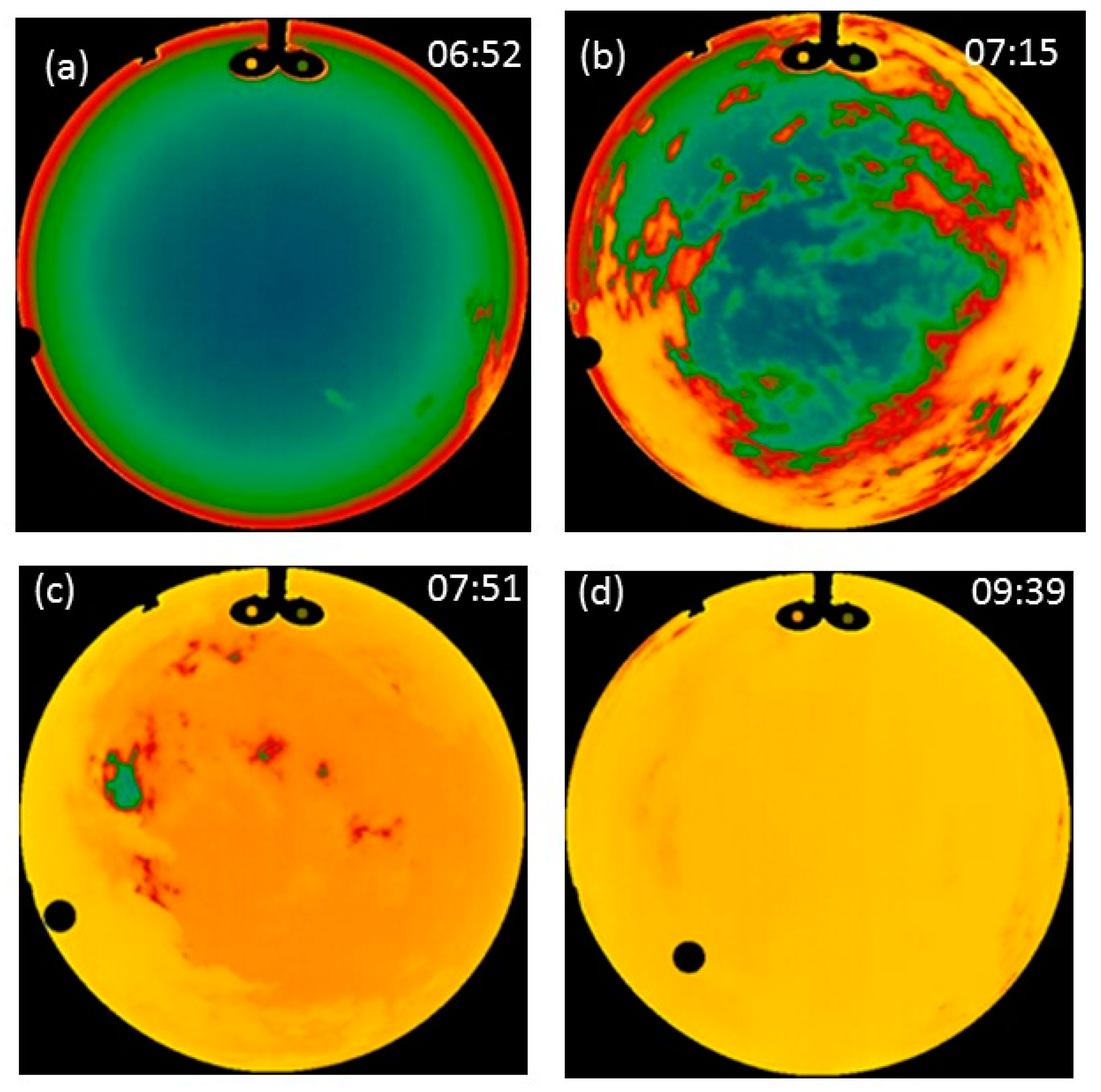
Figure 12.
Sky image on 1 March 2021. (a) 06:52—The very initial buildup phase. The sky begins to cover from the northwest direction. (b) 07:15—In the middle of the buildup phase. The original buildup direction is still apparent. (c) 07:51—At the end of the buildup phase. Some isolated clear sky patches are clearly seen. (d) 09:39—The cloud covers the sensor’s entire field of view.

Figure 13.
The backscattered Doppler Lidar during the fog events of 4 Janaury 2021–6 January 2021 in Nes Ziona.
Figure 13.
The backscattered Doppler Lidar during the fog events of 4 Janaury 2021–6 January 2021 in Nes Ziona.

Figure 14.
Evolution of the fog in time during the morning of 6 Jan 2021. (a): Visibility range. (b): Temperature (Ness Ziona) and relative humidity (Beit Dagan). (c): Droplets size distribution.
Figure 14.
Evolution of the fog in time during the morning of 6 Jan 2021. (a): Visibility range. (b): Temperature (Ness Ziona) and relative humidity (Beit Dagan). (c): Droplets size distribution.

Figure 15.
(a): StreamLine XR Lidar measurement of β during the fog event of 6 January 2021 between 4 a.m. to 7 a.m. local time. (b): Calculated values of β according to the Lidar equation based on mass extinction and backscatter coefficients.
Figure 15.
(a): StreamLine XR Lidar measurement of β during the fog event of 6 January 2021 between 4 a.m. to 7 a.m. local time. (b): Calculated values of β according to the Lidar equation based on mass extinction and backscatter coefficients.

Publisher’s Note: MDPI stays neutral with regard to jurisdictional claims in published maps and institutional affiliations. |
© 2021 by the authors. Licensee MDPI, Basel, Switzerland. This article is an open access article distributed under the terms and conditions of the Creative Commons Attribution (CC BY) license (https://creativecommons.org/licenses/by/4.0/).
Share and Cite
MDPI and ACS Style
Ronen, A.; Tzadok, T.; Rostkier-Edelstein, D.; Agassi, E. Fog Measurements with IR Whole Sky Imager and Doppler Lidar, Combined with In Situ Instruments. Remote Sens. 2021, 13, 3320. https://0-doi-org.brum.beds.ac.uk/10.3390/rs13163320
AMA Style
Ronen A, Tzadok T, Rostkier-Edelstein D, Agassi E. Fog Measurements with IR Whole Sky Imager and Doppler Lidar, Combined with In Situ Instruments. Remote Sensing. 2021; 13(16):3320. https://0-doi-org.brum.beds.ac.uk/10.3390/rs13163320
Chicago/Turabian StyleRonen, Ayala, Tamir Tzadok, Dorita Rostkier-Edelstein, and Eyal Agassi. 2021. "Fog Measurements with IR Whole Sky Imager and Doppler Lidar, Combined with In Situ Instruments" Remote Sensing 13, no. 16: 3320. https://0-doi-org.brum.beds.ac.uk/10.3390/rs13163320
Note that from the first issue of 2016, this journal uses article numbers instead of page numbers. See further details here.