Improving Potato Yield Prediction by Combining Cultivar Information and UAV Remote Sensing Data Using Machine Learning

Abstract

Accurate high-resolution yield maps are essential for identifying spatial yield variability patterns, determining key factors influencing yield variability, and providing site-specific management insights in precision agriculture. Cultivar differences can significantly influence potato (Solanum tuberosum L.) tuber yield prediction using remote sensing technologies. The objective of this study was to improve potato yield prediction using unmanned aerial vehicle (UAV) remote sensing by incorporating cultivar information with machine learning methods. Small plot experiments involving different cultivars and nitrogen (N) rates were conducted in 2018 and 2019. UAV-based multi-spectral images were collected throughout the growing season. Machine learning models, i.e., random forest regression (RFR) and support vector regression (SVR), were used to combine different vegetation indices with cultivar information. It was found that UAV-based spectral data from the early growing season at the tuber initiation stage (late June) were more correlated with potato marketable yield than the spectral data from the later growing season at the tuber maturation stage. However, the best performing vegetation indices and the best timing for potato yield prediction varied with cultivars. The performance of the RFR and SVR models using only remote sensing data was unsatisfactory (R² = 0.48–0.51 for validation) but was significantly improved when cultivar information was incorporated (R² = 0.75–0.79 for validation). It is concluded that combining high spatial-resolution UAV images and cultivar information using machine learning algorithms can significantly improve potato yield prediction than methods without using cultivar information. More studies are needed to improve potato yield prediction using more detailed cultivar information, soil and landscape variables, and management information, as well as more advanced machine learning models.

1. Introduction

Potato (Solanum tuberosum L.) is a high-yield food crop with high added values. It originated in the Andes Mountains of southern Peru [1]. It is resistant to cold, drought, and barrenness, and has high unit input production capacity and strong adaptability [2].

At present, there are 160 countries in the world that grow and produce potatoes, making it very important for world food security [3]. Potato ranks as the fourth largest food crop in the world after rice (Oryza sativa L.), wheat (Triticum aestivum L.), and maize (Zea mays L.) [4]. Similar to other crops, in potato crop production management, accurate high-resolution yield maps are imperative to identify spatial yield variability patterns within commercial fields, determine the key factors affecting yield, and provide management practice insights [5].

Currently, available potato yield monitors are less accessible and the potato yield maps generated from existing yield monitors show low accuracy and inconsistency, resulting in incorrect interpretation of on-farm yield variability [6]. The major influencing factors for the inaccuracy of the potato yield maps produced by the yield monitors include yield sensor calibration, mud, clods or rock separation, operating errors, and data post-processing or cleaning [7]. As a result, yield monitor applications on potato farms are limited. To address these issues, developing a new alternative approach to timely and accurately estimate potato yields would help potato producers make better management decisions.

Remote sensing has been utilized extensively in precision agriculture for in-season crop growth monitoring and yield prediction [8,9]. Vegetation indices (VIs) calculated from remote sensing images are used to correlate to yield variability through statistical and machine learning models. The normalized difference vegetation index (NDVI) is one of the most widely used VIs to evaluate vegetation status and crop yield estimation [5,10]. Nevertheless, its success is strongly influenced by other factors including soil background, crop type, and light conditions [11]. Multi-temporal remote sensing monitoring across the growing seasons can uniquely offer insights into yield formation processes [12,13]. Although some positive results have been reported in potato yield prediction [14], the uncertainties of using only remote sensing data to estimate crop yield limit the application of the model [5,14,15].

Potato yield is typically associated with seed quality as well as site-specific interactions between cultivars and environment conditions. The effects of soil type [16], nutrients [17,18], crop management practices [19,20], cultivar [21,22], seed quality [1,23], and weather conditions [24,25,26] on potato production have been explored extensively. Recent studies that incorporated multi-source data in yield prediction and nitrogen (N) recommendations have achieved better results than studies based on remote sensing data alone. In addition, machine learning technology has been adopted for crop yield prediction [27,28] because it can model both linear and non-linear relationships, and can more easily incorporate ancillary data in the process to improve yield prediction [29]. For example, Salvador et al. [15] highlighted the importance of combining moderate resolution imaging spectroradiometer (MODIS) time series NDVI data with meteorological data for large scale potato yield forecasting. Gómez et al. [6] found that the machine learning methods together with Sentinel-2 data could be used for potato yield prediction and pattern analysis.

In recent years, unmanned aerial vehicle (UAV) technology has shown great potential in precision agriculture. Most previous studies using UAVs have focused on estimating crop biomass, leaf area index (LAI), chlorophyll content, plant height, and N status [27,30,31,32]. For potato biomass and yield prediction, Li et al. [27] combined VIs derived from UAV-based hyperspectral imagery and crop height derived from UAV-based red, green, and blue (RGB) spectral data using random forest regression (RFR) and partial least square regression (PLSR) models. They found that the RFR model performed better than the PLSR model. However, studies evaluating the effects of different cultivars on the performance of UAV-based multispectral imagery for potato yield prediction to potentially improve the yield prediction by incorporating the cultivar information are still very limited. Therefore, the overall goal of this study was to improve potato yield prediction using UAV-based multispectral images and machine learning methods by coupling them with cultivar information. The specific objectives were to (1) evaluate the potential of using only UAV-based multispectral images to estimate the potato yield of different cultivars; (2) analyze the effect of cultivars on the potato yield estimation models based on UAV remote sensing; and (3) evaluate the potential of improving potato yield mapping by incorporating cultivar information with machine learning models.

2. Materials and Methods

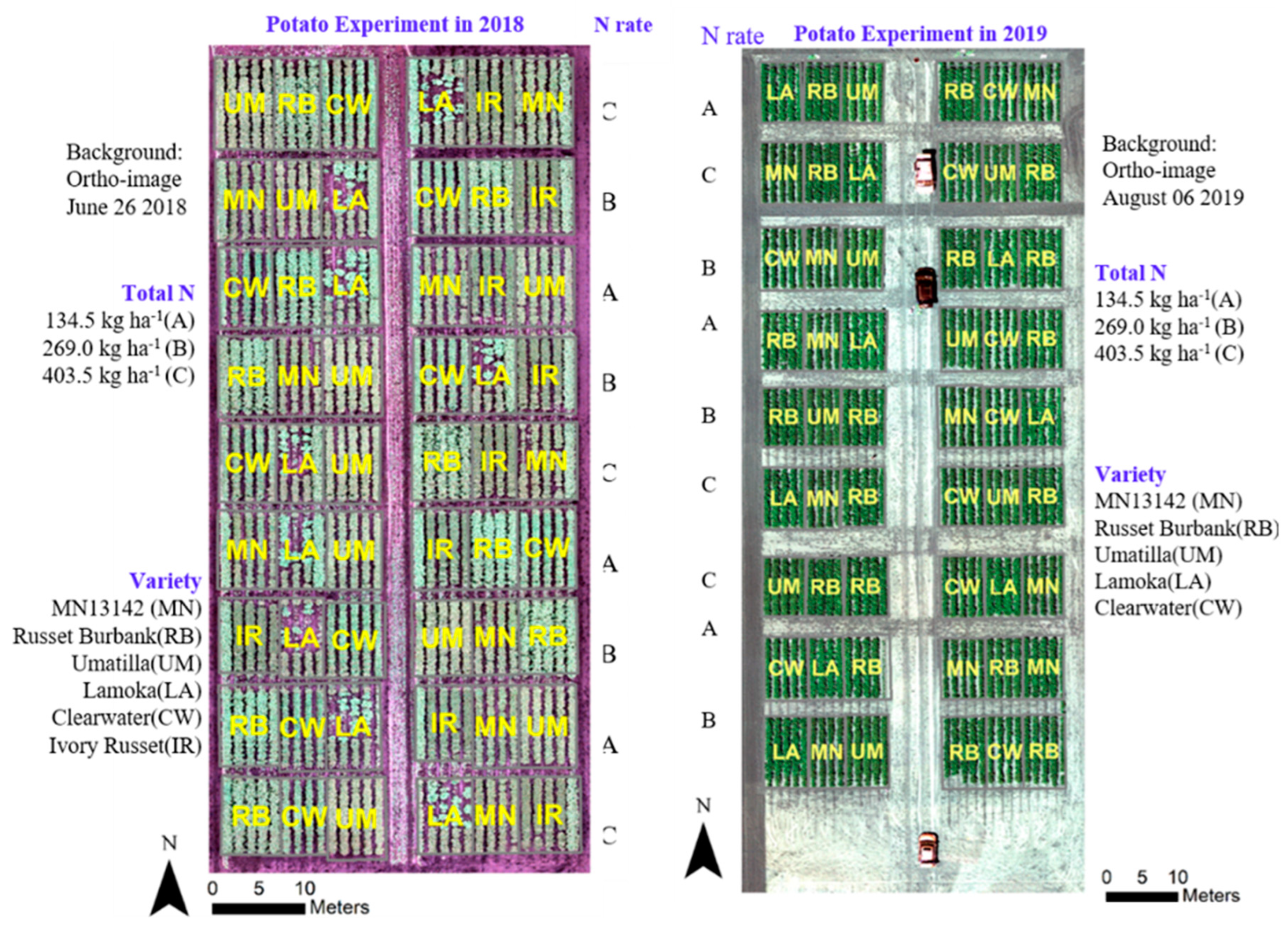
2.1. Small-Plot N x Cultivar Study

The potato N fertilization rate and cultivar studies were conducted at the Sand Plain Research Farm, Becker, Minnesota, with a Hubbard loamy sand soil (sandy, mixed, and frigid Entic Hapludolls) in 2018 and 2019. In this study, four (Russet Burbank, Umatilla Russet, Ivory Russet, and Clearwater Russet) and five (Russet Burbank, Umatilla Russet, Clearwater Russet, Lamoka, and MN13142) cultivars representing different maturity groups that were planted in 2018 and 2019, respectively. The details of the field experiments are shown in Figure 1 and

Table 1. The details of the field experiments and unmanned aerial vehicle (UAV) remote sensing image collection in 2018 and 2019.

Sensing Date	Days after Planting	GDDs to Sensing Date	Cultivar	Abbreviation	Planting Date	Harvesting Date
2018
26 June 2018	44	469	Clearwater Russet Russet Burbank Umatilla Russet Ivory Russet	CW RB UM IR	14 May 2018	25 September 2018
10 July 2018	58	622
18 July 2018	66	766
2 August 2018	81	919
2019
26 June 2019	52	302	Clearwater Russet Russet Burbank Umatilla Russet Lamoka MN12142	CW RB UM LA MN	6 May 2019	27 September 2019
23 July 2019	79	475
6 August 2019	92	593
19 August 2018	106	752

. A randomized complete block design with three replications was used. In 2018, the potatoes were planted on May 14 and harvested on September 25. In 2019, potatoes were planted on May 6 and harvested on September 27. Each cultivar was subjected to three N rate treatments at 134.5, 269.0 and 403.5 kg ha⁻¹. All plots received 45 kg N ha⁻¹ as diammonium phosphate (18-46-0) at planting in a band 0.08 m to the side and 0.05 m below the seed tuber. At emergence, N was side-dressed at 90.0, 125.0, and 269.0 kg N ha⁻¹ as slow-release fertilizer Environmentally Smart Nitrogen (ESN) (Agrium, Inc., Calgary, AB, Canada; 44-0-0) at each specific N rate treatment. The rest of the N fertilizers for the two higher rate treatments were split into four applications of 11.2 and 22.4 kg N ha⁻¹ as urea and ammonium nitrate (28-0-0) to supply 45.0 and 90.0 kg N ha⁻¹ to achieve a total of 269.0 and 403.5 kg N ha⁻¹. At harvest, the vines were killed with desiccant first and then tubers were harvested from the middle two rows of each plot. Tubers were mechanically sorted into different weight classes and grades. A subsample of 25 harvested tubers was used to determine scab infection and hollow heart internal defects. Total tuber yield is the total weight of harvested tubers converted to ton per hectare. Marketable tuber yield was calculated as the weight of all tubers free from defects, disease, crack, and other physiological disorders, converted to ton per hectare. Marketable tuber yield was used in this study.

The growing degree days (GDD) is a useful variable to determine harvest dates and yield in potato [33] and for combining data from different site-years and growth stages [10]. Temperature data was downloaded from the weather station close to the research site. Based on the annual temperature data, GDD was calculated from the planting date to each sensing date following Equation (1):

$$GDD={{\displaystyle \sum }}^{}\frac{T_{max}+T_{min}}{2}-7℃$$

(1)

$T_{max}$ represents the daily maximum temperature. $T_{min}$ represents the daily minimum temperature. 7 ^oC is the base temperature [33].

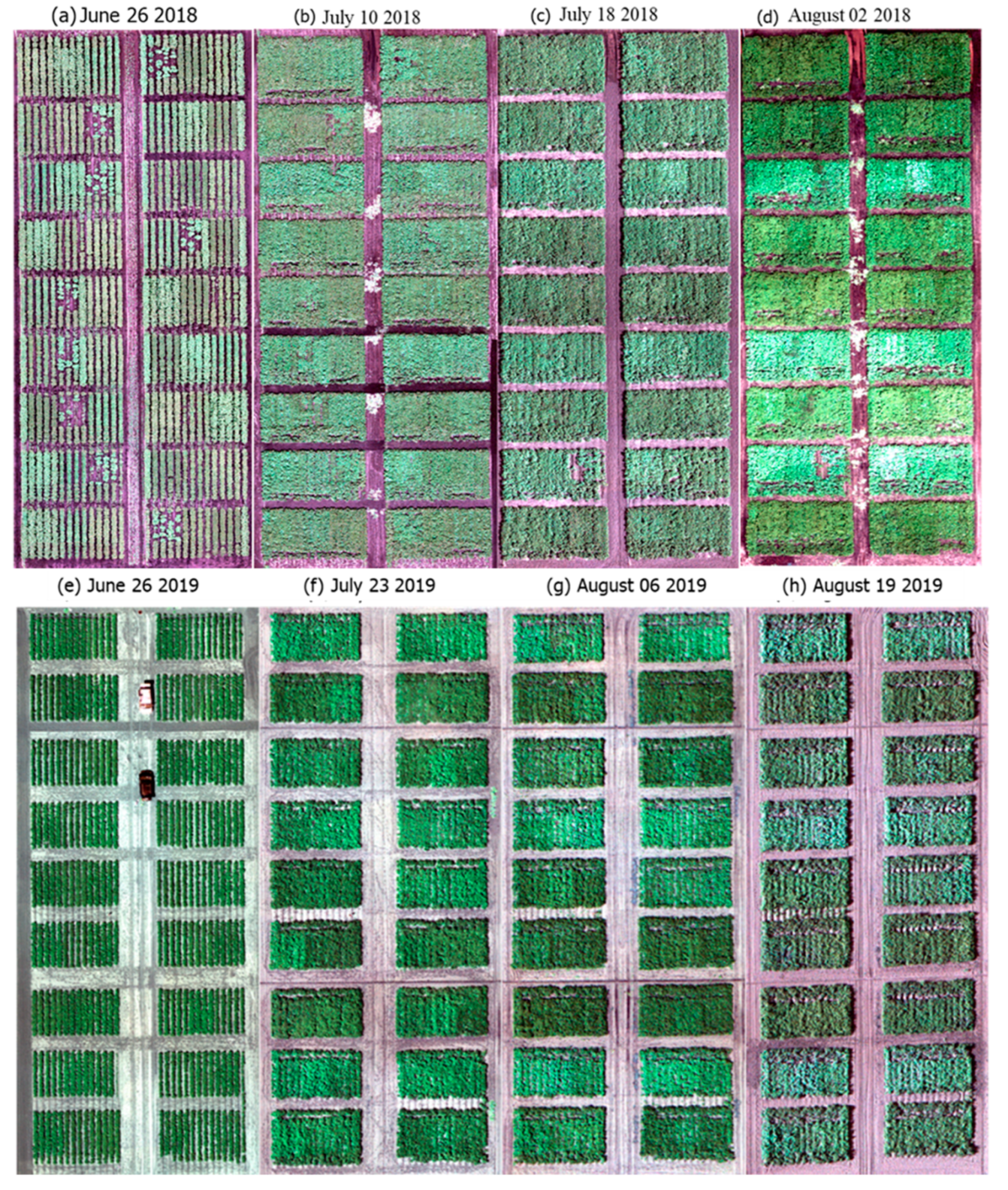
2.2. UAV System and Flight Parameters

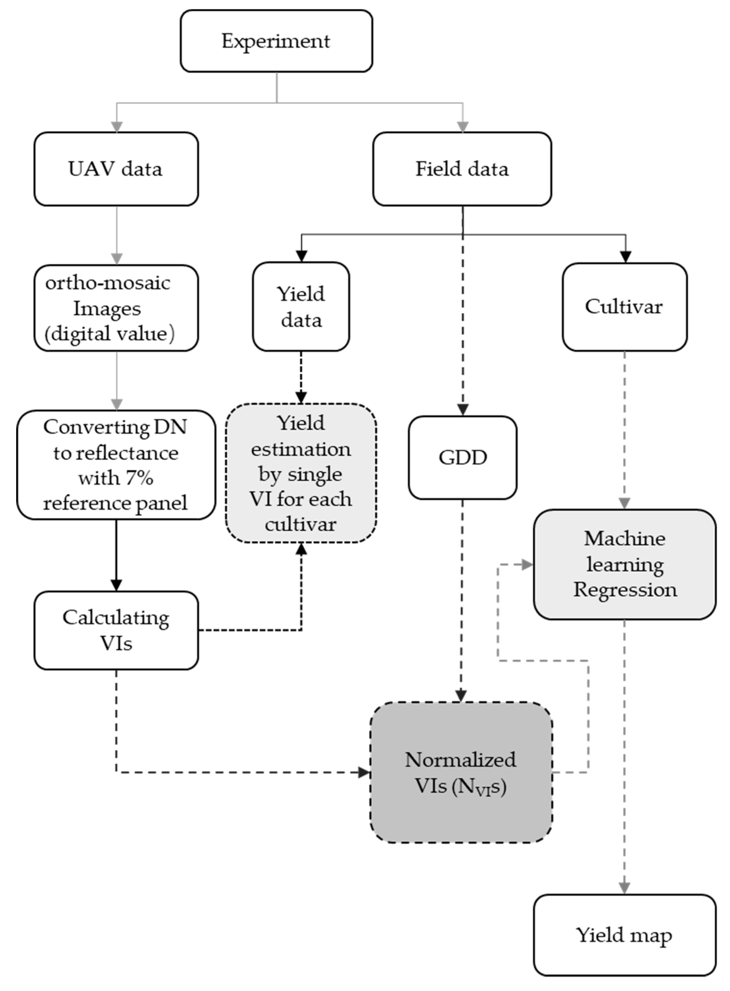
The imagery used to monitor potato growth in these field trails was collected by a GEMS multispectral camera (Sentek Systems LLC, Minneapolis, MN, USA) mounted on a DJI Inspire 2 quadcopter. The UAV flight speed was 6 m s⁻¹. The GEMS camera has four wide spectral bands with the following center wavelengths and full-width, half-maximum (FWHM) bandwidths: Blue (450 nm center, 101 nm FWHM bandwidth), Green (553 nm center, 101 nm FWHM bandwidth), Red (615 nm center, 114 nm FWHM bandwidth), and NIR (811 nm center, 135 nm FWHM bandwidth). The camera has a 35° horizontal field of view and can collect high spatial-resolution images with a ground sampling distance of approximately 2 cm from 40 m above the ground. The Drone Survey iOS flight planning application (Sentek Systems LLC, Minneapolis, MN, USA) was used to prepare flight paths for image collection that covered the trial areas with the desired speed, height, and sidelap. The survey flights used in this study had a minimum forward overlap of 85% and a minimum sidelap of 75%. The GEMS camera has an embedded navigation system that recorded camera position and orientation data at the precise instants that images were taken. The Cheetah software package (Sentek Systems LLC, Minneapolis, MN, USA) was used to process the GEMS imagery with embedded position and orientation data to generate 3D reconstructions, elevation maps, and vegetation index maps, along with the VNIR ortho-mosaic images that were used in this study.

Three reference panels with reflectance values of 7%, 16%, and 27% were put near the experiments during each flight and used to compute surface reflectance from digital number measurements according to Equation (2). The digital number values of the near infrared band became saturated during the later growing season (data collected in July and August), thus only the reference panel with 7% reflectance was used in the data analysis.

$$\frac{R_{ROI}}{D{N}_{ROI}}=\frac{R_{panel}}{D{N}_{panel}}$$

(2)

$R_{ROI}$ represents the average reflectance in a given band in a region of interest (ROI). $D{N}_{ROI}$ represents the digital number values in the ortho-mosaic images, averaged over the ROI. $R_{panel}$ is the reflectance of a reference panel. $D{N}_{panel}$ is the digital number value of the reference panel in the ortho-mosaic images. Reflectance values were averaged over each plot in the trial for analysis. The UAV multispectral images of the fields on different sensing dates are shown in Figure 2.

2.3. Data Analysis

Selected VIs were calculated based on the multispectral UAV images (

Table 2. The definition of the variables used in this study.

Vegetation Index	Abbreviation	Formula	Reference
Difference Vegetation Index	DVI	$DVI=NIR-Red$	[35]
Enhanced Vegetation Index	EVI	$\mathrm{EVI}=2.5*\frac{\left(NIR-Red\right)}{\left(NIR+6*Red\right)-7.5*Blue+1}$	[36]
Green Atmospherically Resistant Index	GARI	$\mathrm{GARI}=\frac{NIR-\left[Green-\gamma \left(Blue-Red\right)\right]}{NIR+\left[Green-\gamma \left(Blue-Red\right)\right]}$	[37]
Green Difference Vegetation Index	GDVI	$\mathrm{GDVI}=\mathrm{NIR}-\mathrm{Green}$	[38]
Modified Triangular Vegetation Index	MTVI	$\mathrm{MTVI}=1.2\left[1.2\left(NIR-Green\right)-2.5\left(\mathrm{Red}-\mathrm{Green}\right)\right]$	[36]
Modified Triangular Vegetation Index-Improved	MTVII	$\mathrm{MTVII}=\frac{1.5\left[1.2\left(NIR-Green\right)-2.5\left(Red-Green\right)\right]}{\sqrt{{\left(2NIR+1\right)}^2-\left(6NIR-5\sqrt{Red}\right)-0.5}}$	[39]
Optimized Soil Adjusted Vegetation Index	OSAVI	$\mathrm{OSAVI}=\frac{1.5\left(NIR-Red\right)}{\left(NIR+Red+0.16\right)}$	[40]
Red Green Ratio Index	RGRI	$\mathrm{RGRI}=\frac{{{\displaystyle \sum }}_{i=600}^{699}{R}_i}{{{\displaystyle \sum }}_{i=500}^{599}{R}_j}$	[41]
Renormalized Difference Vegetation Index	RDVI	$\mathrm{RDVI}=\frac{\left(NIR-Red\right)}{\left(\sqrt{NIR+Red}\right)}$	[42]
Simple Ratio	SR	$\mathrm{SR}=\frac{NIR}{Red}$	[43]
Soil Adjusted Vegetation Index	SAVI	$\mathrm{SAVI}=\frac{1.5\left(NIR-Red\right)}{NIR+red+0.5}$	[44]
Sum Green Index	SGI	$\mathrm{SGI}=\frac{{{\displaystyle \int }}_{i=500}^{600}{R}_i}{100}$	[45]
Transformed Difference Vegetation Index	TDVI	$\mathrm{TDVI}=\sqrt{0.5+\frac{\left(NIR-Red\right)}{\left(NIR+Red\right)}}$	[46]
Visible Atmospherically Resistant Index	VARI	$\mathrm{VARI}=\frac{Green-Red}{Green+Red\_Blue}$	[47]
Green Normalized Difference Vegetation Index	GNDVI	$\mathrm{GNDVI}=\frac{NIR-Green}{NIR+Green}$	[37]
Normalized Difference Vegetation Index	NDVI	$\mathrm{NDVI}=\frac{NIR-Red}{NIR+Red}$	[48]

NIR: reflectance data of the NIR band. Red: reflectance data of the red band. Green: reflectance data of the green band. Blue: reflectance data of the blue band. $R_i$ indicates the reflectance data at wavelength i nm.

). These VIs were normalized using GDD (N_VI), which is particularly useful when combining data from different site-years and growth stages [10,34]. The N_VI was computed by dividing the VI data by the accumulated GDD from planting to sensing, as shown in Equation (3).

$${\mathrm{N}}_{VI}=\frac{VI}{GDD}$$

(3)

Simple regression models were used to determine the relationship (linear, power, quadratic, or exponential) between each vegetation index and potato tuber yield using Statistical Package for the Social Sciences version 18.0 (SPSS 18.0) (SPSS Inc., Chicago, IL, USA). In addition, two machine learning algorithms, i.e., support vector regression (SVR) and RFR, performed well for crop yield prediction in a previous study [28]. Both of them were used to predict potato yield in this research. The SVR and RFR were implemented using the scikit-learn Python ML library.

Random forests consist of decision trees and provide two algorithms, namely mean decrease impurity and mean decrease accuracy, to calculate the importance of features. The mean decrease impurity is calculated to split the dataset into two so that similar response values end up in the same set. Impurity is the measure based on which the (locally) optimal condition is chosen. For regression trees, impurity is the variance. The impurity decrease from each feature can be averaged and the features can be ranked according to this measure [49,50]. The mean decrease impurity algorithm was implemented by the scikit-learn package (https://scikit-learn.org/stable/, accessed on 21 July 2021). Furthermore, the mean decrease accuracy algorithm is used to pass the out-of-band (OOB) samples down the tree and record the prediction accuracy. A variable is then selected and its values in the OOB samples were randomly permuted. OOB samples were passed down the tree and the accuracy was computed again. A decrease in accuracy obtained by this permutation was averaged over all trees for each variable and provided the importance of that variable (the higher the decrease, the higher the importance) [50]. The mean decrease accuracy was calculated by the ELI5 package in Python library (https://eli5.readthedocs.io/en/latest/, accessed on 21 July 2021).

Support vector regression (SVR) is characterized by the use of kernels, sparse solution, and Vapnik–Chervonenkis control of the margin, as well as the numbers of support vectors [51]. SVR has been proven to be an effective tool for real-value function estimation. As a supervised-learning approach, SVR trains using a symmetrical loss function, which equally penalizes high and low misestimates. It has excellent generalization capability with high prediction accuracy [52]. Therefore, they were used in this study to evaluate the potential of coupling UAV multispectral data with cultivar information in potato yield estimation. Cultivar information was pre-processed into dummy variables and introduced in the machine learning models together with the selected four N_VI data to build the inter-annual yield prediction model.

The analysis process flow diagram of this study is given in Figure 3.

In addition to a separate analysis of different years, growth stages, and cultivars, the small plot data from different years were also pooled together, of which 75% was used for model calibration and 25% for validation. The agreement between the observed and predicted parameters was evaluated using the coefficient of determination (R²), root mean square error (RMSE), mean absolute error (MAE), and relative absolute error (RAE) in prediction, as shown in Equations (4)–(7). The models with the largest R² and the lowest RMSE (t ha⁻¹), MAE (t ha⁻¹), and RAE (%) in prediction were identified.

$$R^2=1-\frac{{{\displaystyle \sum }}_{i=1}^n{\left(y_i^m-y_i^p\right)}^2}{{{\displaystyle \sum }}_{i=1}^n{\left(y_i^m-y_i^a\right)}^2}$$

(4)

$$\mathrm{RMSE}=\sqrt{\frac{1}{n}{{\displaystyle \sum }}_{i=1}^n{\left(y_i^m-y_i^p\right)}^2 }$$

(5)

$$\mathrm{MAE}=\frac{1}{n}{{\displaystyle \sum }}_{i=1}^n\left|\left(y_i^m-y_i^p\right)\right|$$

(6)

$$\mathrm{RAE}=\frac{{{\displaystyle \sum }}_{i=1}^n\left|y_i^m-y_i^p\right|}{{{\displaystyle \sum }}_{i=1}^n\left|y_i^a-y_i^m\right|}$$

(7)

$y_i^m$ represents the actual potato yield data (t ha⁻¹) of the i sample. $y_i^p$ represents the predicted potato tuber yield data (t ha⁻¹) of the i sample by the yield estimation model. $y_i^a$ indicates the mean value of the actual potato marketable yield (t ha⁻¹) dataset. n is the sample size while i is the sample number.

3. Results

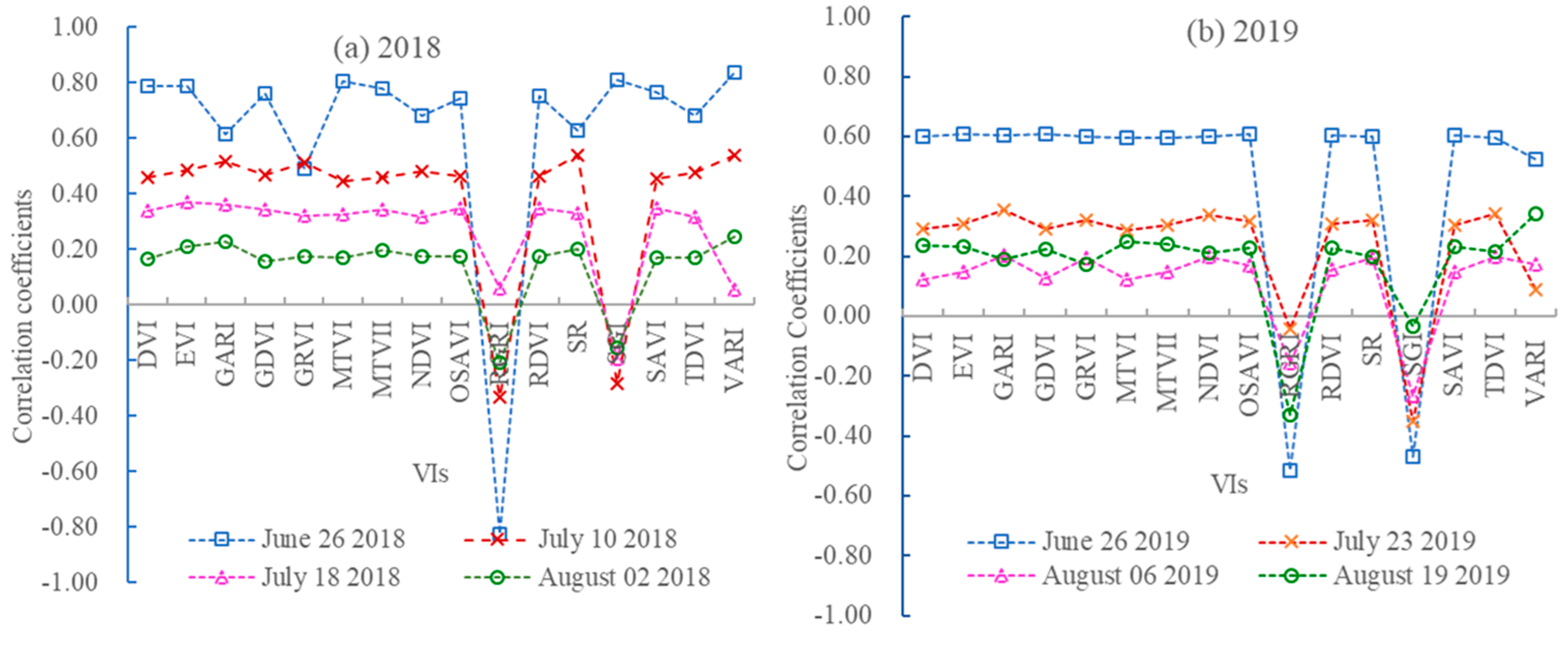
3.1. Correlation Analysis between Potato Tuber Yield and VIs

The correlation coefficients between potato tuber yield and VIs varied throughout the growth period (Figure 4). In general, the VIs collected in late June at the tuber initiation stage had the best relationship with the potato marketable yield across years, with the best correlation coefficients in June and the worst in August at the tuber maturation stage (Figure 2). In June, many VIs showed significant correlation with yield data at the p < 0.05 level. The Visible Atmospherically Resistance Index (VARI) had the highest correlation coefficients with yield on June 26 and July 10 in 2018. On other sensing dates in 2018, the VIs and yield did not show a significant correlation. In 2019, there was a significant correlation between the Enhanced Vegetation Index (EVI) and yield on June 26, while no significant correlation was found for the other three sensing dates.

3.2. Simple Regression Models for Potato Tuber Yield Prediction

Yield models were developed based on the most strongly correlated VIs with tuber yield for each cultivar at each growth stage. The details of these models are presented in

Table 3. Best performing vegetation indices on different dates for predicting potato marketable yield in 2018.

Cultivar	VI	Equation	R2	RMSE (t ha−1)
		26 June 2018
Across	VARI	y = −900.34x2 + 567.93x − 7.95	0.71	6.48
CW	SGI	y = −335891.19x2 + 47518.15x − 1650.71	0.52	3.15
IR	VARI	y = −10022.70x2 + 2049.63x − 69.14	0.56	2.30
RB	RGRI	y = −2762.77x2 + 4348.04x − 1651.24	0.31	3.85
UR	GARI	y = −344.43x2 + 453.48x − 77.34	0.80	2.87
		10 July 2018
Across	VARI	y = −23878x2 + 16263x − 2720.2	0.30	9.97
CW	GARI	y = 1786.07x2 + 22122.07x − 601.38	0.09	4.17
IR	SGI	y = −56579.29x2 + 11496.50x − 547.67	0.75	1.73
RB	RGRI	y = 9735.48x2 − 11551.28x + 3474.325	0.34	3.75
UR	GARI	y = −6688.93x2 + 8443.64x − 2612.62	0.78	3.03
		18 July 2018
Across	/	/	/	/
CW	GNDVI	y = −1319.83x2 + 1584.31x − 445.35	0.26	3.76
IR	SGI	y = −26227.30x2 + 2488.14x − 22.33	0.79	1.5
RB	RGRI	y = 4735.16x2 − 7802.20x + 3259.107	0.60	2.92
UR	GARI	y = 1388.37x2 − 1235.45x + 313.01	0.74	3.27
		2 August 2018
Across	/	/	/	/
CW	TDVI	y = −3730.29x2 + 7957.54x − 4213.78	0.22	3.85
IR	GDVI	y = −1545.97x2 + 1843.42x − 512.79	0.73	1.79
RB	MTVI	y = −4172.66x2 + 2319.06x − 264.868	0.41	3.55
UR	GARI	y = −0.43x2 + 97.41x − 0.085	0.77	3.08

Across: the model developed by across cultivar data for each sensing date. Abbreviations: CW, Clearwater Russet; IR, Ivory Russet; RB, Russet Burbank; UR, Umatilla Russet; SGI, Sum Green Index; VARI, Visible Atmospherically Resistant Index; GARI, Green Atmospherically Resistant Index; TDV, Transformed Difference Vegetation Index; SAVI, Soil Adjusted Vegetation Index; RGRI, red–green ratio index; GNDVI, Green Normalized Difference Vegetation Index; and MTVI, Modified Triangular Vegetation Index.

and

Table 4. Best performing vegetation indices on different dates for predicting potato marketable yield in 2019.

Cultivar	VI	Equation	R2	RMSE (t ha−1)
26 June 2019
Across	EVI	y = −1220.38x2 + 750.36x − 70.75	0.40	4.84
CW	VARI	y = −11263.45x2 + 719.95x + 21.67	0.57	2.65
LA	SGI	y = −40983.18x2 + 4455.11 − 75.02	0.30	2.33
MN	/	/	/	/
RB	RGRI	y = −1398.99x2 + 2669.64x − 1222.89	0.35	2.85
UR	RGRI	y = 4628.27x2 − 8586.01x + 4022.49	0.50	2.02
23 July 2019
Across	/	/	/	/
CW	/	/	/	/
LA	SGI	y = 126137.77x2 − 9151.45x + 201.97	0.22	2.47
MN	/	/	/	/
RB	/	/	/	/
UR	SGI	y = 290331.87x2 − 22661.40x + 482.60	0.55	1.93
		6 August 2019
Across	/	/	/	/
CW	/	/	/	/
LA	VARI	y = 741.65x2 − 218.60x + 49.338	0.51	1.96
MN	/	/	/	/
RB	/	/	/	/
UR	SGI	y = 31294.42x2 − 3787.65x + 154.94	0.75	1.45
		19 August 2019
Across	/	/	/	/
CW	/	/	/	/
LA	SGI	y = −23103.32x2 + 3446.58x − 88.404	0.59	1.80
MN	/	/	/	/
RB	/	/	/	/
UR	SGI	y = 44215.48x2 − 6167.62x + 255.25	0.70	1.55

Across: the model developed by across cultivar data for each sensing date. Abbreviations: CW, Clearwater Russet; IR, Ivory Russet; RB, Russet Burbank; UR, Umatilla Russet; MN, MN12142; LA, Lamoka; SGI, Sum Green Index; VARI, Visible Atmospherically Resistant Index; and RGVI, Green Ratio Vegetation Index.

.

In 2018, the model based on VARI had an R² of 0.71 and an RMSE of 6.48 t ha⁻¹ on June 26. On July 10, the R² of the VARI-based model was 0.30 and the RMSE was 9.97 t ha⁻¹. On July 18 and August 2, there was no model that could achieve significant results. In 2019, the model based on EVI had an R² of 0.40 and an RMSE of 4.84 t ha⁻¹, whereas no models were significant for the other three sensing dates.

In order to investigate the correlation between the VIs and potato marketable yield of each cultivar, we developed the single VI-based model of potato yield prediction for each cultivar and investigated the variation of the correlation at different growth stages.

Apparently, the models performed better for cultivars Ivory Russet and Umatilla Russet at each growth stage in 2018, with R² ranging from 0.56 to 0.80. As for Clearwater Russet, the early growth stage was the best stage to predict yield with an R² value of 0.52. For Russet Burbank, the best stage to predict marketable yield was July 18.

In 2019, for Lamoka, the yield estimation model was the best in August as compared with those in June and July. For MN12142, there was no significant model to predict the yield across the growth stages. For Russet Burbank, the model on June 26 had an R² of 0.35 and an RMSE of 2.85 t ha⁻¹. These results are not consistent with those in 2018. For Umatilla Russet, the model in each growth stage performed well, with the R² values greater than 0.50, which is consistent with the results of 2018.

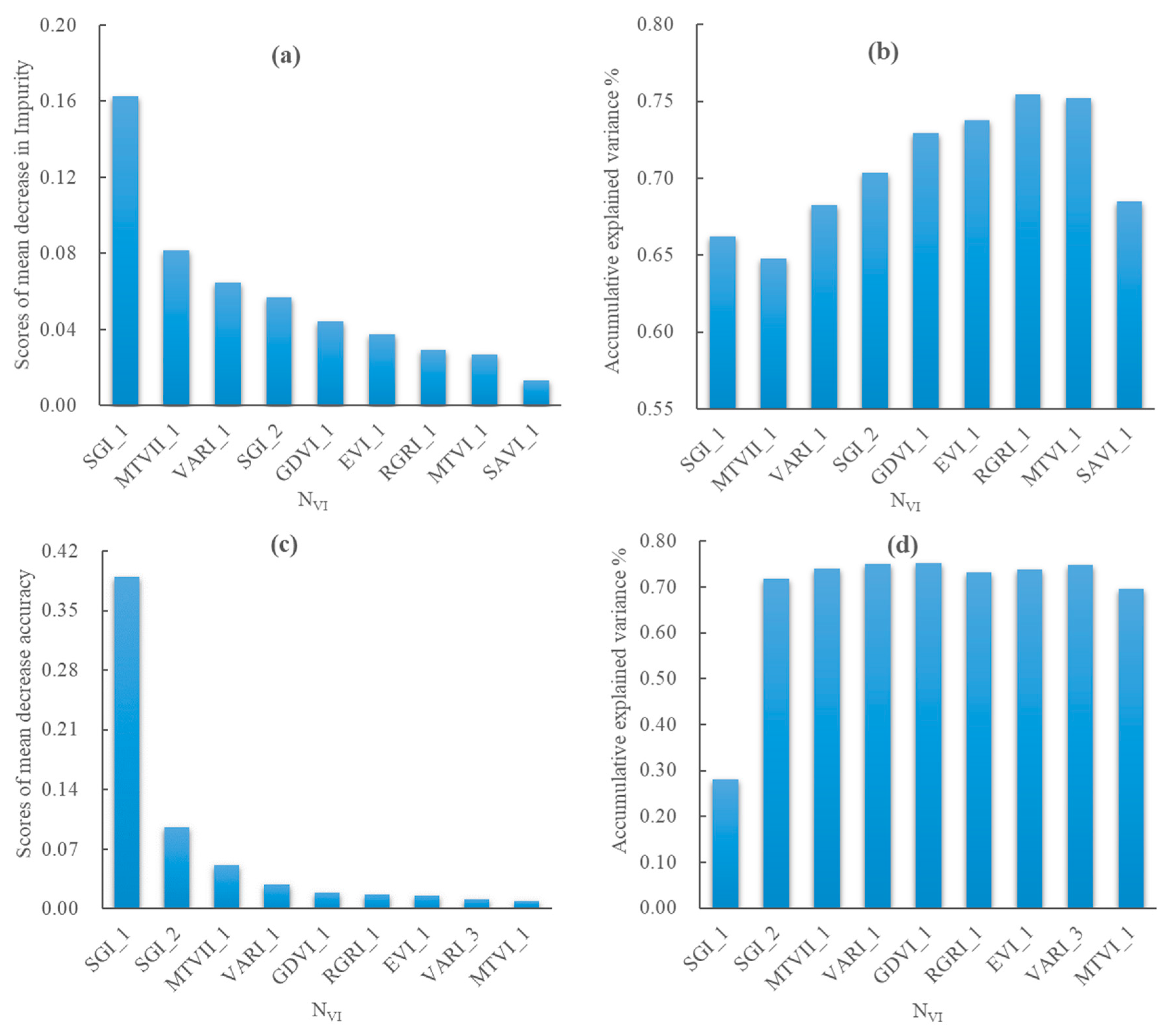
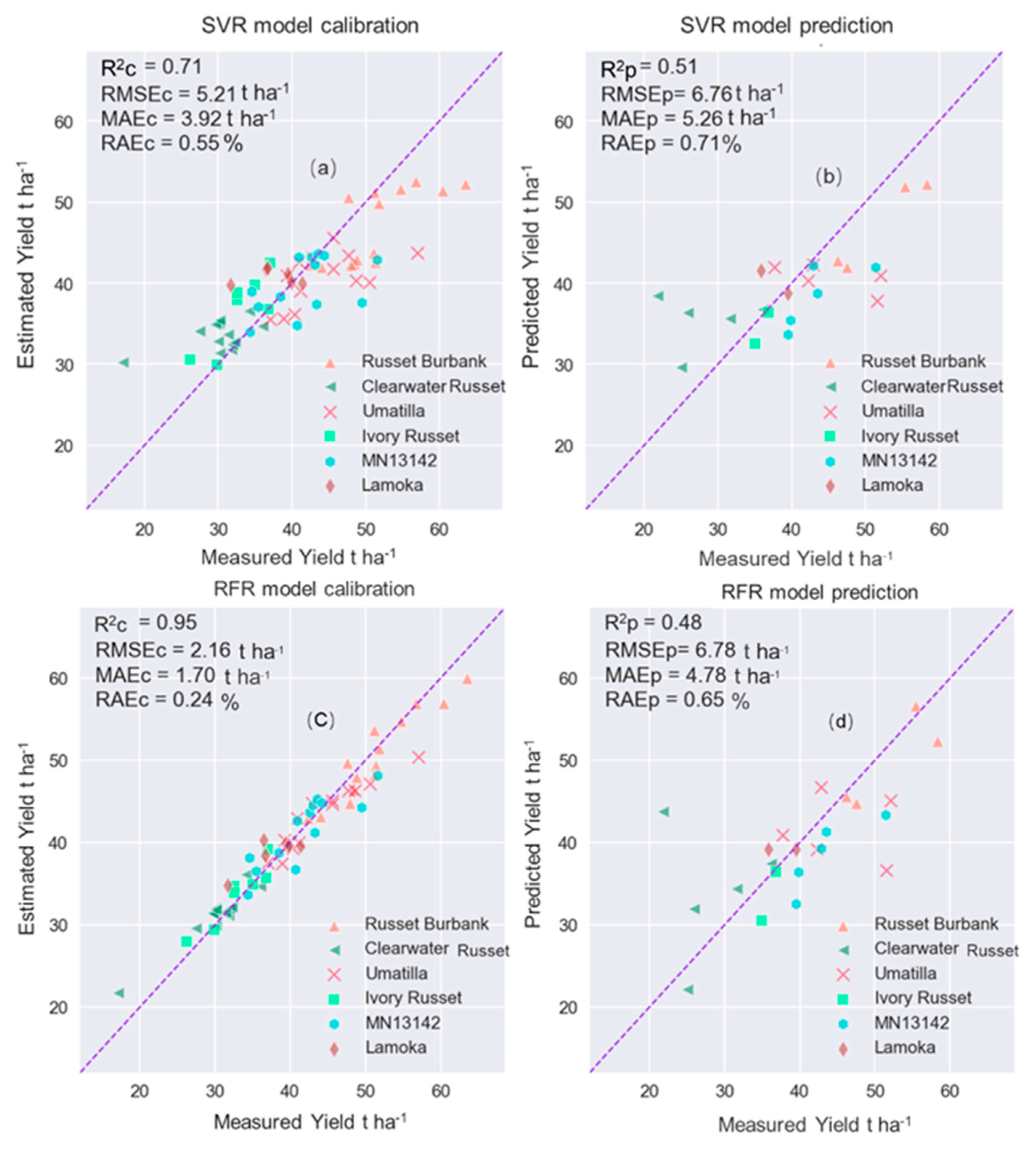
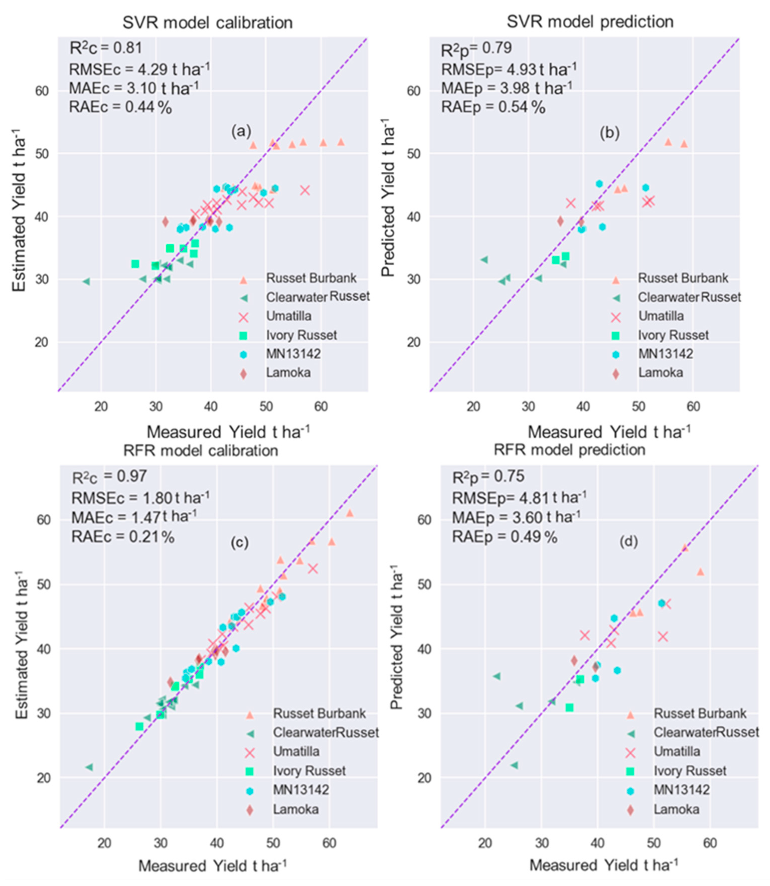
3.3. Machine Learning Models

To reduce the influence of different dates, years, and sites, the N_VI data were calculated from the VIs and GDDs. General models that integrated potato cultivar information and N_VI data were constructed using machine learning methods.

Two feature selection algorithms (mean decrease impurity and mean decrease accuracy) were implemented to select the best feature subset. Figure 5 shows the descending scores of N_VI data derived by a preliminary random forest method, in addition to the two feature selection algorithms and accumulative variance of the features.

From the cumulative histogram (Figure 5b), we can see that the first seven variables contributed over 75% of the accumulative variance of the model. However, the accumulative variance decreased when adding more inputs than the first seven variables. The first seven variables with high scores in both mean decrease in impurity and mean decrease accuracy were selected. Therefore, the Normalized Modified Triangular Vegetation Index improved (N_MTVII). The Normalized Sum Green Index (N_SGI) and normalized VARI (N_VARI) obtained on the first sensing date, in addition to the N_SGI acquired on the second sensing date, were chosen for the machine learning processes.

According to the above-selected variables, the RFR and SVR models were developed. Figure 6 shows the scatterplots between the estimated yield and measured yield. Although the RFR method performed better than the SVR in the calibration models, similar performance was found in the prediction or validation results.

The scatterplots in Figure 7 show the relationships between the measured yield and the estimated yield obtained by the two machine learning models using the pooled data based on the selected VIs and cultivar information.

Evidently, the incorporation of cultivar information into the UAV remote sensing-based models improved potato yield prediction (Figure 6 and Figure 7). The R² of the prediction model increased from 0.51 to 0.79 and from 0.48 to 0.75 for the SVR and RFR methods, respectively. The RFR model had a smaller RMSE, MAE, and RAE than the SVR model in both the calibration and prediction processes. However, the R² value (0.97) of the RFR calibration model was much higher than that (0.75) of the RFR prediction model, whereas consistent R² values were identified for the SVR calibration and prediction models, indicating that the RFR method might be more affected by the size of the dataset and larger calibration dataset might lead to higher accuracy of the RFR model. The RFR yield prediction model was applied to the UAV images to produce potato yield distribution maps in 2018 and 2019, which are shown in Figure 8.

4. Discussion

This study indicated that the accuracy of the potato tuber yield estimation model was closely related to the sensing time and cultivar information. For the combined cultivar dataset, the Pearson correlation analysis indicated that UAV images collected in late June (44–52 days after planting dates) during the stage of plant full vegetative growth and tuber initiation were better for potato yield prediction than during later growth stages, similar to the findings reported by some previous studies [5,10]. For the machine learning models, the VIs obtained in June were more important for yield estimation than the VIs obtained later during the growing season. A similar result was reported at the field scale [10].

The yield predictive models based on VIs are cultivar and sensing date-specific [5,10]. Potato cultivar had an important effect on the yield estimation models. In general, for cultivars Clearwater Russet and Russet Burbank, UAV image data obtained early in the growing season (late June) was more suitable for yield estimation. For cultivars Ivory Russet and Lamoka, the UAV image data obtained later in the growing season performed better. The yield of MN13142 could not be estimated via single vegetation index-based models. For Umatilla Russet, the entire growing season was suitable for yield prediction. A crop growth model simulation study indicated that potato tuber yield responses to changes in the cultivar parameters was specific to the environment [53]. Cultivars differed mostly in terms of plant N uptake dynamics and belowground biomass in field experiments [54]. The canopy morphology of variable potato cultivars and nitrogen rates were different [27]. Medium maturing and late maturing cultivars were included in this study and it was noticed that there were differences in vine senescence later in the season among different maturity cultivars. The rate of greenness loss [55] and lodging property [27] for some cultivars also affected the performance of VIs in yield estimation in the late growth stages [55]. Senescence affected the vegetation coverage, which in turn influenced the variation of VIs and their relationships with potato yield [5]. The cultivars that grew well during the whole growth season tended to have a better correlation between the VIs and yield.

The spectral bands around 500, 550, and 720 nm were important when assessing potato agronomic properties [56]. The Sum Green Index (SGI) based on green band reflectance information in June was the most important feature for the pooled dataset. The SGI was the reflectance information of the green band. The good performance of SGI across cultivars in the early and middle growth stages should be attributed to the much less absorption of chlorophyll in the green region compared to those in the blue or red regions [57]. The correlation between yields and chlorophyll in the field conditions may explain the importance of the green band in the early growth stage [55,58]. The priority of the green band in crop yield estimation was also reported in other crops (e.g., maize) [59]. The high correlation between VARI and yield was also noticeable for each cultivar, especially on the first sensing date. A similar conclusion was reported for corn yield estimation using multispectral images by Garcia-Martinez et al. [60].

The results of this study indicated that single VI-based models are cultivar-specific. Although machine learning models were developed by combining several VIs, the accuracy of the yield models was still low (Figure 5), similar to a previous study [27]. The machine learning models combining optimal VIs and cultivar information [53] showed good potential in yield estimation, which is consistent with several previous studies [6,11,28]. SVM and RFR are two popular machine learning models used in precision agriculture and remote sensing data analysis, and one was found to perform better than the other in different studies [6,19,31]. In this study, although the RFR performed better than the SVR for the calibration process of a larger dataset, they performed similarly for a smaller validation dataset. The performance of both models was significantly improved when cultivar information was added. This clearly demonstrates the importance of adding other important variables in addition to the use of sensing data. Other studies have also found that apart from sensor data, the incorporation of plant height [27], meteorological data [15], and other related information improved the accuracy of yield estimation models.

In this study, cultivar information was incorporated in the machine learning models as dummy variables. This is an initial attempt. Further studies are needed to use more detailed information to represent cultivar differences, such as maturity days, growing GDDs, or growing degree units. More studies are needed to develop potato yield prediction models that incorporate more ancillary information together with remote sensing data using more advanced machine learning algorithms.

5. Conclusions

This study investigated the potential of using UAV-multispectral images coupled with cultivar information to predict potato yield and generate potential field-scale yield maps. The maturity days for each cultivar were different and the responses of potato tuber yield to the N rate also varied with cultivars. The best performing VIs and best sensing timing for potato yield prediction varied with cultivars. For cultivars Clearwater Russet and Russet Burbank, the best sensing date was in late June (44–52 days after planting). For cultivars Ivory Russet and Lamoka, the optimum sensing time was later in the growing season. For Umatilla Russet, VI-based models performed consistently well across the growing season, while no suitable models were found for cultivar MN13142 based on single VI at any of the growth stages. The R²s of single VI-based models for different cultivars varied from 0.22 to 0.80. In general, UAV images acquired early in the season (late June) were more correlated with potato yield across cultivars. Using machine learning models (RFR and SVR) to combine selected VIs with cultivar information could significantly improve the accuracy of potato yield prediction (R² = 0.75–0.79 for validation) compared with machine learning models only using VIs (R² = 0.48–0.51 for validation). More studies are needed to improve potato yield prediction using more detailed cultivar information, weather data, soil and landscape variables, and management information.

References

1. Haverkort, A.; Struik, P. Yield levels of potato crops: Recent achievements and future prospects. Field Crop. Res. 2015, 182, 76–85. [Google Scholar] [CrossRef]
2. Batool, T.; Ali, S.; Seleiman, M.F.; Naveed, N.H.; Ali, A.; Ahmed, K.; Abid, M.; Rizwan, M.; Shahid, M.R.; Alotaibi, M.; et al. Plant growth promoting rhizobacteria alleviates drought stress in potato in response to suppressive oxidative stress and antioxidant enzymes activities. Sci. Rep. 2020, 10, 1–19. [Google Scholar] [CrossRef] [PubMed]
3. Ayyub, C.M.; Haidar, M.W.; Zulfiqar, F.; Abideen, Z.; Wright, S.R. Potato tuber yield and quality in response to different nitrogen fertilizer application rates under two split doses in an irrigated sandy loam soil. J. Plant Nutr. 2019, 42, 1850–1860. [Google Scholar] [CrossRef]
4. Eid, M.A.M.; Abdel-Salam, A.A.; Salem, H.M.; Mahrous, S.E.; Seleiman, M.F.; Alsadon, A.A.; Solieman, T.H.I.; Ibrahim, A.A. Interaction Effects of Nitrogen Source and Irrigation Regime on Tuber Quality, Yield, and Water Use Efficiency of Solanum tuberosum L. Plants 2020, 9, 110. [Google Scholar] [CrossRef] [Green Version]
5. Al-Gaadi, K.A.; Hassaballa, A.; Tola, E.; Kayad, A.; Madugundu, R.; Alblewi, B.; Assiri, F. Prediction of Potato Crop Yield Using Precision Agriculture Techniques. PLoS ONE 2016, 11, e0162219. [Google Scholar] [CrossRef]
6. Gómez, D.; Salvador, P.; Sanz, J.; Casanova, J.L. Potato Yield Prediction Using Machine Learning Techniques and Sentinel 2 Data. Remote Sens. 2019, 11, 1745. [Google Scholar] [CrossRef] [Green Version]
7. Davenport, J.; Redulla, C.; Hattendorf, M.; Evans, R.; Boydston, R. Potato Yield Monitoring on Commercial Fields. HortTechnology 2002, 12, 289–296. [Google Scholar] [CrossRef] [Green Version]
8. Wang, X.; Tian, S.; Lou, H.; Zhao, R. A reliable method for predicting bioethanol yield of different varieties of sweet potato by dry matter content. Grain Oil Sci. Technol. 2020, 3, 110–116. [Google Scholar] [CrossRef]
9. Yang, W.; Nigon, T.; Hao, Z.; Paiao, G.D.; Fernández, F.G.; Mulla, D.; Yang, C. Estimation of corn yield based on hyperspectral imagery and convolutional neural network. Comput. Electron. Agric. 2021, 184, 106092. [Google Scholar] [CrossRef]
10. Zaeen, A.A.; Sharma, L.; Jasim, A.; Bali, S.; Buzza, A.; Alyokhin, A. In-season potato yield prediction with active optical sensors. Age 2020, 3. [Google Scholar] [CrossRef] [Green Version]
11. Gómez, D.; Salvador, P.; Sanz, J.; Casanova, J.L. New spectral indicator Potato Productivity Index based on Sentinel-2 data to improve potato yield prediction: A machine learning approach. Int. J. Remote. Sens. 2021, 42, 3426–3444. [Google Scholar] [CrossRef]
12. Luo, S.; He, Y.; Li, Q.; Jiao, W.; Zhu, Y.; Zhao, X. Nondestructive estimation of potato yield using relative variables derived from multi-period LAI and hyperspectral data based on weighted growth stage. Plant Methods 2020, 16, 1–14. [Google Scholar] [CrossRef]
13. Sivarajan, S. Estimating yield of irrigated potatoes using aerial and satellite. Ph.D. Thesis, Utah State University, Logan, UT, USA, 2011. [Google Scholar]
14. Zhao, Y.; Chen, X.; Cui, Z.; Lobell, D.B. Using satellite remote sensing to understand maize yield gaps in the North China Plain. Field Crop. Res. 2015, 183, 31–42. [Google Scholar] [CrossRef]
15. Salvador, P.; Gómez, D.; Sanz, J.; Casanova, J.L. Estimation of Potato Yield Using Satellite Data at a Municipal Level: A Machine Learning Approach. ISPRS Int. J. Geo-Inf. 2020, 9, 343. [Google Scholar] [CrossRef]
16. Redulla, C.A.; Davenport, J.R.; Evans, R.G.; Hattendorf, M.J.; Alva, A.K.; Boydston, R.A. Relating potato yield and quality to field scale variability in soil characteristics. Am. J. Potato Res. 2002, 79, 317–323. [Google Scholar] [CrossRef]
17. Rosen, C.J.; Bierman, P.M. Potato Yield and Tuber Set as Affected by Phosphorus Fertilization. Am. J. Potato Res. 2008, 85, 110–120. [Google Scholar] [CrossRef]
18. Torabian, S.; Farhangi-Abriz, S.; Qin, R.; Noulas, C.; Sathuvalli, V.; Charlton, B.; Loka, D. Potassium: A Vital Macronutrient in Potato Production—A Review. Agronomy 2021, 11, 543. [Google Scholar] [CrossRef]
19. Sun, C.; Feng, L.; Zhang, Z.; Ma, Y.; Crosby, T.; Naber, M.; Wang, Y. Prediction of End-Of-Season Tuber Yield and Tuber Set in Potatoes Using In-Season UAV-Based Hyperspectral Imagery and Machine Learning. Sensors 2020, 20, 5293. [Google Scholar] [CrossRef]
20. Zhang, S.; Wang, H.; Sun, X.; Fan, J.; Zhang, F.; Zheng, J.; Li, Y. Effects of farming practices on yield and crop water productivity of wheat, maize and potato in China: A meta-analysis. Agric. Water Manag. 2021, 243, 106444. [Google Scholar] [CrossRef]
21. Eaton, T.E.; Azad, A.K.; Kabir, H.; Siddiq, A.B. Evaluation of Six Modern Varieties of Potatoes for Yield, Plant Growth Parameters and Resistance to Insects and Diseases. Agric. Sci. 2017, 8, 1315–1326. [Google Scholar] [CrossRef] [Green Version]
22. Tessema, L.; Mohammed, W.; Abebe, T. Evaluation of Potato (Solanum tuberosum L.) Varieties for Yield and Some Agronomic Traits. Open Agric. 2020, 5, 63–74. [Google Scholar] [CrossRef] [Green Version]
23. de Oliveira, J.S.; Brown, H.E.; Gash, A.; Moot, D.J. Yield and weight distribution of two potato cultivars grown from seed potatoes of different physiological ages. N. Zealand J. Crop. Hortic. Sci. 2016, 45, 91–118. [Google Scholar] [CrossRef]
24. Sharma, L.K.; Bali, S.K.; Dwyer, J.D.; Plant, A.B.; Bhowmik, A. A Case Study of Improving Yield Prediction and Sulfur Deficiency Detection Using Optical Sensors and Relationship of Historical Potato Yield with Weather Data in Maine. Sensors 2017, 17, 1095. [Google Scholar] [CrossRef] [Green Version]
25. Dahal, K.; Li, X.-Q.; Tai, H.; Creelman, A.; Bizimungu, B. Improving Potato Stress Tolerance and Tuber Yield Under a Climate Change Scenario—A Current Overview. Front. Plant Sci. 2019, 10, 563. [Google Scholar] [CrossRef]
26. Wagg, C.; Hann, S.; Kupriyanovich, Y.; Li, S. Timing of short period water stress determines potato plant growth, yield and tuber quality. Agric. Water Manag. 2021, 247, 106731. [Google Scholar] [CrossRef]
27. Li, B.; Xu, X.; Zhang, L.; Han, J.; Bian, C.; Li, G.; Liu, J.; Jin, L. Above-ground biomass estimation and yield prediction in potato by using UAV-based RGB and hyperspectral imaging. ISPRS J. Photogramm. Remote Sens. 2020, 162, 161–172. [Google Scholar] [CrossRef]
28. Van Klompenburg, T.; Kassahun, A.; Catal, C. Crop yield prediction using machine learning: A systematic literature review. Comput. Electron. Agric. 2020, 177, 105709. [Google Scholar] [CrossRef]
29. Wang, X.; Miao, Y.; Dong, R.; Zha, H.; Xia, T.; Chen, Z.; Kusnierek, K.; Mi, G.; Sun, H.; Li, M. Machine learning-based in-season nitrogen status diagnosis and side-dress nitrogen recommendation for corn. Eur. J. Agron. 2021, 123, 126193. [Google Scholar] [CrossRef]
30. Li, S.; Yuan, F.; Ata-Ui-Karim, S.T.; Zheng, H.; Cheng, T.; Liu, X.; Tian, Y.; Zhu, Y.; Cao, W.; Cao, Q. Combining Color Indices and Textures of UAV-Based Digital Imagery for Rice LAI Estimation. Remote Sens. 2019, 11, 1763. [Google Scholar] [CrossRef] [Green Version]
31. Zheng, H.; Cheng, T.; Zhou, M.; Li, D.; Yao, X.; Tian, Y.; Cao, W.; Zhu, Y. Improved estimation of rice aboveground biomass combining textural and spectral analysis of UAV imagery. Precis. Agric. 2019, 20, 611–629. [Google Scholar] [CrossRef]
32. Zha, H.; Miao, Y.; Wang, T.; Li, Y.; Zhang, J.; Sun, W.; Feng, Z.; Kusnierek, K. Improving Unmanned Aerial Vehicle Remote Sensing-Based Rice Nitrogen Nutrition Index Prediction with Machine Learning. Remote Sens. 2020, 12, 215. [Google Scholar] [CrossRef] [Green Version]
33. Worthington, C.M.; Hutchinson, C.M. Accumulated growing degree days as a model to determine key developmental stages and evaluate yield and quality of potato in Northeast Florida. Proc. Fla. State Hortic. Soc. 2005, 118, 98–101. [Google Scholar]
34. Zaeen, A.A.; Sharma, L.K.; Jasim, A.; Bali, S.; Buzza, A.; Alyokhin, A. Yield and quality of three potato cultivars under series of nitrogen rates. Agrosyst. Geosci. Environ. 2020, 3. [Google Scholar] [CrossRef]
35. Tucker, C.J. Red and photographic infrared linear combinations for monitoring vegetation. Remote Sens. Environ. 1979, 8, 127–150. [Google Scholar] [CrossRef] [Green Version]
36. Huete, A.; Didan, K.; Miura, T.; Rodriguez, E.P.; Gao, X.; Ferreira, L.G. Overview of the radiometric and biophysical performance of the MODIS vegetation indices. Remote Sens. Environ. 2002, 83, 195–213. [Google Scholar] [CrossRef]
37. Gitelson, A.A.; Kaufman, Y.J.; Merzlyak, M.N. Use of a green channel in remote sensing of global vegetation from EOS-MODIS. Remote Sens. Environ. 1996, 58, 289–298. [Google Scholar] [CrossRef]
38. Sripada, R.P.; Heiniger, R.W.; White, J.G.; Meijer, A.D. Aerial color infrared photography for determining early in-season nitrogen requirements in corn. Agron. J. 2006, 98, 968–977. [Google Scholar] [CrossRef]
39. Haboudane, D.; Miller, J.R.; Pattey, E.; Zarco-Tejada, P.; Strachan, I. Hyperspectral vegetation indices and novel algorithms for predicting green LAI of crop canopies: Modeling and validation in the context of precision agriculture. Remote Sens. Environ. 2004, 90, 337–352. [Google Scholar] [CrossRef]
40. Rondeaux, G.; Steven, M.; Baret, F. Optimization of soil-adjusted vegetation indices. Remote Sens. Environ. 1996, 55, 95–107. [Google Scholar] [CrossRef]
41. Gamon, J.; Surfus, J.S. Assessing leaf pigment content and activity with a reflectometer. New Phytol. 1999, 143, 105–117. [Google Scholar] [CrossRef]
42. Roujean, J.-L.; Breon, F.-M. Estimating PAR absorbed by vegetation from bidirectional reflectance measurements. Remote Sens. Environ. 1995, 51, 375–384. [Google Scholar] [CrossRef]
43. Birth, G.S.; McVey, G.R. Measuring the Color of Growing Turf with a Reflectance Spectrophotometer 1. Agron. J. 1968, 60, 640–643. [Google Scholar] [CrossRef]
44. Huete, A. A soil-adjusted vegetation index (SAVI). Remote Sens. Environ. 1988, 25, 295–309. [Google Scholar] [CrossRef]
45. Lobell, D.B.; Asner, G.P. Hyperion studies of crop stress in Mexico. In Proceedings of the 12th Annual JPL Airborne Earth Science Workshop, Pasadena, CA, USA, 24–28 February 2003. [Google Scholar]
46. Bannari, A.; Asalhi, H.; Teillet, P. Transformed difference vegetation index (TDVI) for vegetation cover mapping. In Proceedings of the IEEE International Geoscience & Remote Sensing Symposium, Toronto, ON, Canada, 24–28 June 2002; Volume 3055, pp. 3053–3055. [Google Scholar]
47. Gitelson, A.A.; Stark, R.; Grits, U.; Rundquist, D.; Kaufman, Y.; Derry, D. Vegetation and soil lines in visible spectral space: A concept and technique for remote estimation of vegetation fraction. Int. J. Remote. Sens. 2002, 23, 2537–2562. [Google Scholar] [CrossRef]
48. Rouse, J.; Hass, R.; Schell, J.; Deering, D. Monitoring vegetation systems in the great plains with ERTS. In Proceedings of the Third ERTS Symposium, Washington, DC, USA, 10–14 December 1973; pp. 309–317. [Google Scholar]
49. Breiman, L.; Friedman, J.H.; Olshen, R.A.; Stone, C.J. Classification and Regression Trees. Belmont, CA: Wadsworth. Int. Group 1984, 432, 151–166. [Google Scholar]
50. Breiman, L. Random Forests. Mach. Learn. 2001, 28. [Google Scholar]
51. Sheykhmousa, M.; Mahdianpari, M.; Ghanbari, H.; Mohammadimanesh, F.; Ghamisi, P.; Homayouni, S. Support Vector Machine Versus Random Forest for Remote Sensing Image Classification: A Meta-Analysis and Systematic Review. IEEE J. Sel. Top. Appl. Earth Obs. Remote. Sens. 2020, 13, 6308–6325. [Google Scholar] [CrossRef]
52. Awad, M.M. Toward Precision in Crop Yield Estimation Using Remote Sensing and Optimization Techniques. Agriculture 2019, 9, 54. [Google Scholar] [CrossRef] [Green Version]
53. Kleinwechter, U.; Gastelo, M.; Ritchie, J.; Nelson, G.; Asseng, S. Simulating cultivar variations in potato yields for contrasting environments. Agric. Syst. 2016, 145, 51–63. [Google Scholar] [CrossRef]
54. Maltas, A.; Dupuis, B.; Sinaj, S. Yield and Quality Response of Two Potato Cultivars to Nitrogen Fertilization. Potato Res. 2018, 61, 97–114. [Google Scholar] [CrossRef]
55. Ramírez, D.; Yactayo, W.; Gutierrez, R.; Mares, V.; De Mendiburu, F.; Posadas, A.; Quiroz, R. Chlorophyll concentration in leaves is an indicator of potato tuber yield in water-shortage conditions. Sci. Hortic. 2014, 168, 202–209. [Google Scholar] [CrossRef]
56. Sun, N.; Wang, Y.; Gupta, S.K.; Rosen, C.J. Nitrogen Fertility and Cultivar Effects on Potato Agronomic Properties and Acrylamide-forming Potential. Agron. J. 2019, 111, 408–418. [Google Scholar] [CrossRef]
57. Clevers, J.G.P.W.; Kooistra, L. Mapping canopy chlorophyll content of potatoes by Sentinel-2 as simulated with RapidEye images. In Proceedings of the Sentinel-2 for Science Workshop, Frascati, Italy, 20 May 2014; p. 7. [Google Scholar]
58. Jurečka, F.; Lukas, V.; Hlavinka, P.; Semerádová, D.; Žalud, Z.; Trnka, M. Estimating Crop Yields at the Field Level Using Landsat and MODIS Products. Acta Univ. Agric. Silvic. Mendel. Brun. 2018, 66, 1141–1150. [Google Scholar] [CrossRef] [Green Version]
59. Panda, S.S.; Ames, D.P.; Panigrahi, S. Application of Vegetation Indices for Agricultural Crop Yield Prediction Using Neural Network Techniques. Remote Sens. 2010, 2, 673–696. [Google Scholar] [CrossRef] [Green Version]
60. García-Martínez, H.; Flores-Magdaleno, H.; Ascencio-Hernández, R.; Khalil-Gardezi, A.; Tijerina-Chávez, L.; Mancilla-Villa, O.; Vázquez-Peña, M. Corn Grain Yield Estimation from Vegetation Indices, Canopy Cover, Plant Density, and a Neural Network Using Multispectral and RGB Images Acquired with Unmanned Aerial Vehicles. Agriculture 2020, 10, 277. [Google Scholar] [CrossRef]
Figure 1. The layouts of the potato field experiments in 2018 (left) and 2019 (right) involving six cultivars (MN13142 (MN), Russet Burbank (RB), Umatilla Russet (UM), Lamoka (LA), Clearwater Russet (CW), and Ivory Russet (IR)) and three nitrogen rates (A= 134.5 kg ha−1, B = 269.0 kg ha−1, and C = 403.5 kg ha−1).
Remotesensing 13 03322 g001
Figure 2. The true color-composite images of the potato fields during different sensing dates. The true color images collected on 26 June 2018 (a), 10 July 2018 (b), 18 July 2018 (c), 2 August 2018 (d), 26 June 2019 (e), 23 July 2019 (f), 6 August 2019 (g), and 19 August 2019 (h).
Remotesensing 13 03322 g002
Figure 3. The process flow diagram of the study.
Remotesensing 13 03322 g003
Figure 4. The correlation coefficients between vegetation indices and potato marketable tuber yield on different dates during the growing seasons of 2018 (a) and 2019 (b).
Remotesensing 13 03322 g004
Figure 5. The scores of mean decrease in impurity and mean decrease accuracy of the top nine variables and the accumulative explained variance calculated from the random forest algorithm. (a) The scores of mean decrease in impurity; (b) The accumulative explained variance % of the top nine variables selected by the scores of mean decrease in impurity; (c) The scores of mean decrease accuracy; (d) The accumulative explained variance % of the top nine variables selected by the scores of mean decrease accuracy. SGI_1 means the Normalized Sum Green Index (NSGI) calculated by the SGI and GDD on the first sensing date. SGI_2 means the normalized SGI calculated by the SGI and GDD on the second sensing date. VARI_3 indicates the Normalized Visible Atmospherically Resistance Index (NVARI) calculated by the VARI and GDD on the third sensing date. Other normalized VIs have similar meanings.
Remotesensing 13 03322 g005
Figure 6. Relationships between the measured yield and the estimated yield by the SVR and RFR models using the selected NVIs data without including cultivar information. (a) The scatterplot between measured yield data and estimated yield data for calibration dataset by SVR model; (b) The scatterplot between measured yield data and estimated yield data for prediction dataset by SVR model; (c) The scatterplot between measured yield data and estimated yield data for calibration dataset set by RFR model; (d) The scatterplot between measured yield data and predicted yield data for prediction dataset by RFR model.
Remotesensing 13 03322 g006
Figure 7. Relationships between the measured yield and the estimated yield by the SVR and RFR models using the pooled vegetation indices across site-years, sensing dates, and cultivar information. The scatterplot between measured yield and estimated yield for calibration dataset (a) and validation dataset (b) using the SVR model, and for calibration dataset (c) and validation dataset (d) using the RFR model.
Remotesensing 13 03322 g007
Figure 8. The predicted potato yield maps based on the RFR model developed with selected normalized vegetation indices (NVI) and cultivar information for 2018 (left) and 2019 (right).
Remotesensing 13 03322 g008