
High Wind Speed Inversion Model of CYGNSS Sea Surface Data Based on Machine Learning


1
Shanghai Marine Intelligent Information and Navigation Remote Sensing Engineering Technology Research Center, Shanghai Ocean University, Shanghai 201306, China
2
Shanghai Spaceflight Institute of TT&C and Telecommunication, Shanghai 201109, China
*
Author to whom correspondence should be addressed.
Remote Sens. 2021, 13(16), 3324; https://0-doi-org.brum.beds.ac.uk/10.3390/rs13163324
Submission received: 29 June 2021
/
Revised: 13 August 2021
/
Accepted: 19 August 2021
/
Published: 23 August 2021
(This article belongs to the Special Issue Statistical and Machine Learning Models for Remote Sensing Data Mining - Recent Advancements)
Abstract
:In response to the deficiency of the detection capability of traditional remote sensing means (scatterometer, microwave radiometer, etc.) for high wind speed above 25 m/s, this paper proposes a GNSS-R technique combined with a machine learning method to invert high wind speed at sea surface. The L1-level satellite-based data from the Cyclone Global Navigation Satellite System (CYGNSS), together with the European Centre for Medium-Range Weather Forecasts (ECMWF) and the National Centers for Environmental Prediction (NCEP) data, constitute the original sample set, which is processed and trained with Support Vector Regression (SVR), the combination of Principal Component Analysis (PCA) and SVR (PCA-SVR), and Convolutional Neural Network (CNN) methods, respectively, to finally construct a sea surface high wind speed inversion model. The three models for high wind speed inversion are certified by the test data collected during Typhoon Bavi in 2020. The results show that all three machine learning models can be used for high wind speed inversion on sea surface, among which the CNN method has the highest inversion accuracy with a mean absolute error of 2.71 m/s and a root mean square error of 3.80 m/s. The experimental results largely meet the operational requirements for high wind speed inversion accuracy.

1. Introduction
As one of the most serious natural disasters in the world, typhoons are a top priority for scientific research because of their suddenness and destructive power, which bring huge economic losses to human society. Remote sensing technology provides a huge development space for typhoon monitoring and prediction. All microwave remote sensing instruments are struggling to provide reliable high wind speed measurements above 25 m/s. However, few studies have been obtained up to now [1,2,3,4,5]. The Global Navigation Satellite System reflection (GNSS-R) technology uses satellite signals reflected from the Earth’s surface to obtain information of surface characteristics such as sea surface wind speed, so it can be provided with all-weather detection capability [6,7,8,9,10,11]. The main purpose of the Cyclone Global Navigation Satellite System (CYGNSS), launched by the United States in 2016, is to monitor tropical cyclones. It measures sea surface winds in and near the eyewalls of tropical cyclones, typhoons, and hurricanes frequently throughout their life cycle and the data collected can be used to invert wind speeds [12].
Many methods can be used to inverse wind speed. For example, a GNSS-R wind speed inversion method is to extract DDM observables reflecting the wind speed from the delay-Doppler map (DDM) and then build the Geophysical Model Function (GMF) model for wind speed inversion. Some other studies use the matched filter method between simulated DDMs and measured DDMs to inverse wind speed. In addition, the machine learning method is also suitable for wind speed inversion.
In 2014, Clarizia et al. [6] extracted five DDM observables from the United Kingdom disaster monitor constellation (UK-DMC) satellite, namely Delay-Doppler Map Average (DDMA), Delay-Doppler Map Variance (DDMV), Allan DDM Variance (ADDMV), Leading Edge Slope (LES), and Trailing Edge Slope (TES). Different GMF models were established by comparing the five observables with the buoy wind speed provided by the National Data Buoy Center (NDBC). Then, the reverse wind speeds, using each of these GMFs, were combined into a minimum variance estimator. The root mean square error (RMSE) obtained for wind speeds less than 10 m/s was 1.65 m/s. In 2016, Rodriguez et al. [13] used a generalized observable to determine the coefficients of linear combination by the maximum signal-to-noise ratio (MSNR), the minimum variance of the wind speed (MVU), and principal component analysis (PCA). Then, the three wind speed values were compared with the CYGNSS baseline L2 observables. The results show that PCA performs best, but the overall RMS was greater than 4 m/s when the wind speed was greater than 20 m/s. In 2018, Christopher S. Ruf et al. [9] used the observable DDMA and LES from CYGNSS L1 level data to establish the Fully Developed Seas (FDS) GMF and Young Seas/Limited Fetch (YSLF) GMF for different incidence angles at different seas. The knowledge of wind speed inversion algorithm required to establish FDS GMF model comes from [7]. The reference wind speed used to train the FDS GMF were the 10 m-referenced ocean surface wind speeds provided by the ECMWF and the GDAS. The YSLF GMF model was established using the wind speed collected by the stepped frequency microwave radiometer (SFMR) on NOAA P-3 hurricane hunter aircraft. The FDS GMF model was suitable for low-to-moderate wind speeds. On the contrary, the YSLF GMF model was more sensitive to hurricanes. By using FDS GMF to invert wind speed below 20 m/s and comparing with the European Centre for Medium-Range Weather Forecasts (ECMWF), the overall RMSE was about 2 m/s. In addition, compared with SFMR aircraft data, when the wind speed was greater than 20 m/s, the RMSE of the YSLF GMF model inversion wind speed was about 6.5 m/s. In addition, the samples for wind speeds greater than 20 m/s tested numbered only 674.
In 2017, F.Said [14] et al. proposed a method to inverse the maximum hurricane wind speed using the simulated power-versus-delay waveform data of CYGNSS. The CYGNSS end-to-end simulator (E2ES) [7] was used to produce the reference simulated waveforms. The specific process was to compare the simulated waveform with the reference waveform generated over a set of synthetic Willoughby storms with known maximum wind speed (Vmax) through the matched filter, and output the Vmax corresponding to the reference waveform. The Vmax was the retrieved wind speed. Comparing the retrieved Vmax values of 552 hurricane events with the hurricane weather research and forecasting model (HWRF) Vmax and the Best Track for Vmax, the overall bias of wind speed less than 40 m/s was greater than 11 m/s, and the overall bias of wind speed greater than 40 m/s was less than 3 m/s. However, the samples of hurricane wind speed studied were not enough. In 2019, Al-Khaldi, M [15] et al. extended the simulation study of [14] to the use of CYGNSS full DDM. A matched filter approach between normalized simulated DDMs and measured DDMs was applied to inverse storm parameters. The Vmax estimates were inversed by using the data during Hurricane Irma. Compared with the reported National Hurricane Center Best Track forecasts, the RMSE was 6.89 m/s. In 2021, the same team including Al-Khaldi, M [16] carried out a progress update and error analysis on the research performed by [15]. They continued to use the CYGNSS full DDM and proposed to use the synthetic storm model to retrieve wind speed on the basis of [15]. The synthetic storm model included the Willoughby model and Generalized Asymmetric Holland Model (GAHM). The success of inversion was due to the combination of the GAHM model suitable for storms with low levels of development and the Willoughby model suitable for storms with higher levels. The inversion Vmax was obtained by combining the results of the two models. Compared with the Best Track forecasts, the RMSE was 6.05 m/s. The RMSE was partially improved by comparison with the reference [15]. The effects of measurement delay extent on inverse error were also analyzed.
In 2019, Chong Wu et al. [17] used a back propagation (BP) neural network to invert the wind speed from 0 to 30 m/s, based mainly on the DDM data from CYGNSS. The DDM Observables included DDMA, LES, and Bistatic Radar Cross Section (BRCS). The paper used the CYGNSS L2 wind speed data as the reference wind speed. The Pearson correlation coefficient of the inverse wind speed and the CYGNSS wind speed data product was 0.958, the RMSE was 1.86 m/s, and the mean relative error was 2.66%. The feasibility and effectiveness of wind speed inversion using neural network based on DDM was demonstrated. However, the amount of data for wind speeds greater than 20 m/s in the paper was small and the applicability of the neural network for high wind speed data cannot be confirmed. In the same year, Han Gao et al. [18] used eight observables in CYGNSS L1 data (DDMA, LES, TES, specular reflection point position, satellite altitude angle, Scatter Area, delay-Doppler correlation power mean, and Effective Area) to train the model with a BP neural network, and then compared the reverse wind speed with the wind speed data provided by ECMWF. When the wind speed was less than 20 m/s, the RMSE was 1.21 m/s, and the RMSE in the wind speed range of 20~45 m/s was 2.54 m/s. However, this paper only had 4761 wind speed data above 20 m/s, which was not enough for high wind speed training.
In 2020, Jennifer et al. [10] proposed the Artificial Neural Network (ANN) inversion algorithm for wind speed inversion based on CYGNSS satellite data. In this paper, six characteristic parameters (DDMA, LES, Incidence Angle, Range Corrected Gain (RCG) [7], and Latitude and Longitude of the specular point acquisition.) were used to train ANN model, and CYGNSS L2 wind speed data was used as the reference wind speed. The RMSD of wind speed inversion error for the range of 0~32 m/s was 1.51 m/s. However, the wind speeds in the paper mainly focus on 0–20 m/s, and there was not enough research on wind speeds above 20 m/s, thus good inversion results cannot be obtained for tropical storms. In the same year, Sja Wang [19] performed a comparison between neural network and machine learning methods using Tech Demo Sat-1 (TDS-1) satellite DDM map data and ECMWF data for wind speeds in the 3–18 m/s interval. It was verified that the inversion effect of the neural network model had a significant advantage with a 20% performance improvement.
In 2020, Cardellach et al. [20] combined CYGNSS uncalibrated Level-1 bin original observation count with ECMWF/C3S ERA5 reanalysis dataset to obtain specular reflection point wind speed. The study covered hurricane season data for 2018 and 2019. The inversion was carried out by a variational technique based on physical forward model. The inverse wind speed was compared with the background model, other spaceborne sensors, such as NASA Soil Moisture Active Passive (SMAP), ESA Soil Moisture and Ocean Salinity (SMOS), EUMETSAT Advanced Scatterometer on board METOP (ASCAT) A/B, and other organizations’ CYGNSS inverse wind speed. The research showed that this method had the ability to infer wind speed (including hurricane winds). The inverse wind speed was the most consistent with NOAA inversion [21], but the lowest correlation was found between inversion and the official products that were obtained with the YSLF GMF, and the dispersion reached 9.9 m/s. The author expected that this method will work at moderate wind speed, but this method had the possibility of underestimating wind speed.
According to the above research results, it can be found that machine learning has been widely used in the inversion of sea surface wind speed in the field of remote sensing at present; however, relevant studies for high wind speed greater than 20 m/s are relatively lacking [22].
In this paper, we put forward a high wind speed inversion model for CYGNSS data based on machine learning methods for inversion of typhoons. The datasets consist of the CYGNSS measured L1 data published by the National Aeronautics and Space Administration (NASA) and the reanalyzed wind speed datasets of the ECMWF and National Centers for Environmental Prediction (NCEP). Three methods, Support Vector Regression (SVR), the combination of PCA and SVR (PCA-SVR), and Convolutional Neural Networks (CNN), are used to train the wind speed data above 20 m/s. Due to the uneven distribution of samples, the under-sampling method is used to extract data for training. The three models obtained after training are used to inverse the high wind speed during the typhoon Bavi life cycle typhoon in 2020. Compared with the wind speed from ECMWF/NCEP, the inversion results are used to study the performance of the three models.
2. Materials and Methods
2.1. Data Source
2.1.1. CYGNSS
The CYGNSS satellites are a constellation of eight low Earth orbit (LEO) microsatellites launched in 2016. Each satellite is equipped with a right-hand-circular polarization (RHCP) antenna to receive direct signals from the transmitting satellite and two left-hand-circular polarization (LHCP) antennas to receive reflected signals from reflective surfaces such as the sea surface. The specular reflection points collected by the CYGNSS satellite cover approximately ±40° latitude zone in the global area, and the longitude zone is completely covered. CYGNSS seeks to improve weather prediction capabilities by studying the interaction between ocean surface properties, humid atmospheric thermodynamics, radiation, and convective dynamics associated with tropical cyclones [7,9,12,14,15,16,20]. CYGNSS data is encapsulated by NASA in netCDF file format, and this paper used version 2.1 of the CYGNSS Level 1 data (available online at https://podaac.jpl.nasa.gov/dataset/CYGNSS_L1_V2.1, accessed on 8 April 2021), which is the result of the power expression transformed by L0 level DDM [10].
2.1.2. Mean Sea Level Pressure
Mean sea level (MSL) pressure is an important factor affecting typhoon status and its path [23]. This paper uses the MSL pressure reanalysis data product provided by ECMWF’s official website. The MSL pressure reanalysis dataset calculates the atmospheric pressure on the Earth’s surface, including all land, ocean, and inland water, and then adjusts the surface atmospheric pressure height to the height of mean sea level. The spatial resolution of MSL pressure dataset is 0.5°, and the temporal resolution is 1 h.
2.1.3. Global Wind Speed Data
This paper used two different global reanalysis wind speed datasets: ECMWF reanalysis dataset and NCEP reanalysis dataset, mainly to study wind speed data at the 10 m-referenced ocean surface wind speed (u10), using UTC time. ECMWF regularly uses its forecasting models and data assimilation system to reanalyze archived observations and further create global reanalysis datasets describing the recent history of the atmosphere, land, and ocean. The datasets provide sea surface wind speed at a spatial and temporal resolution of 1 h, 0.5°. NCEP adopts a state-of-the-art global data assimilation system and a comprehensive database to quality control and assimilate observations from various sources (ground, ships, radio soundings, wind balloons, aircraft, satellites, etc.) to obtain reanalysis datasets. The datasets provide sea surface wind speed with a temporal and spatial resolution of 1 h, 0.2°. Further using the time, latitude, and longitude of the observed data provided by CYGNSS, the reanalysis datasets are passed through spatial linear interpolation with temporal linear interpolation to obtain the corresponding wind speed in time and space. This paper combined the wind speed reanalysis datasets of ECMWF and NCEP. The data from ECMWF alone were used when the wind speed is less than 20 m/s, and the data from NCEP are used when the wind speed was greater than 20 m/s [9,24,25]. Finally, the wind speed dataset was composed into new datasets according to this criterion, and the new datasets were used as the true wind speed for training and testing.
2.2. Machine Learning Methods
Three methods, SVR, PCA-SVR, and CNN, were used to train the data to obtain three models; the following sections briefly outline the principles of each method.
2.2.1. SVR
SVR can improve the generalization ability of model by seeking structural risk minimization, so as to achieve the minimum empirical risk and confidence interval. Using fewer samples can also obtain good statistical rules. The input data is normalized before the SVR training to prevent training imbalance caused by feature anomalies. Additionally, normalization can also improve the computational speed. The SVR algorithm first symmetrically maps the input data X into a multidimensional space in a nonlinear way and then performs linear programming in that space. The selection of parameters of SVR generally includes three elements: The first is the selection of kernel function, here the radial basis function (RBF) with better smoothing performance is chosen; the second parameter is the selection of penalty factor C; the third parameter is the selection of kernel coefficient gamma value. In order to avoid overfitting and underfitting, this paper uses the grid search method to perform parameter search for C and gamma values when training the model [26,27]. In order to improve the rate of parameter search, the grid search method is adjusted as follows. Firstly, by finding the optimal parameters in a wide range roughly, and then by setting a smaller step size to search again according to this optimal parameter taking range.
The goal of SVR can be formalized as:
where is the normal vector, which determines the direction of the hyperplane. n is the number of samples, C > 0 is the penalty parameter, is the error sensitivity index, and and are slack variables. By using the dual principle and introducing Lagrange multipliers, the above formula is solved:
where and are the Lagrange multipliers, is the radial basis function, and b is the threshold. Equation (2) is a kernel function introduced by the nonlinear SVR to deal with dimensional catastrophes [28].
The preprocessed training data were trained by SVR method, and the gamma value of the model was determined to be 72.50 and C was 0.09 by grid search.
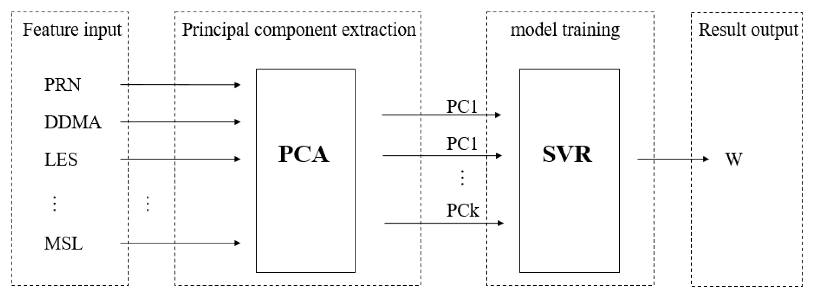
2.2.2. PCA-SVR
Since the number of features tends to increase the model training time, PCA was used here to reduce the dimensionality of SVR input by secondary integration of multidimensional feature covariates in order to reduce the model training time and improve the independence of feature covariates. PCA, as a technique of data dimensionality reduction, can project the original features to the dimension with the maximum amount of projected information as much as possible and ensure the minimum loss of information after dimensionality reduction without affecting the final model prediction results, the processed data are then fed into the SVR for data prediction [29,30].
In the PCA-SVR prediction model, a total of 27 influencing factors were used as input data in this paper. The input training set was processed by PCA to obtain the principal components PC1, PC2, …, and PCk (k ≤ 27) for model prediction, and it was found that the cumulative contribution of the first 13 principal components reached more than 85%, which could replace all feature covariates for model training, so k was 13. Then, the dimensionality reduction data was input into SVR, and the gamma value of the model was determined to be 32.50 and C was 0.37 using the grid search method. Figure 1 shows the structure of the PCA-SVR model.
When the wind speed modeling is completed and enters the wind speed inversion stage, the feature parameters of the CYGNSS test set are normalized and directly multiplied with the corresponding feature vectors to obtain the principal component parameters. Then, the trained model is used for high wind speed inversion and the inversion accuracy of the inverse wind speed is calculated.
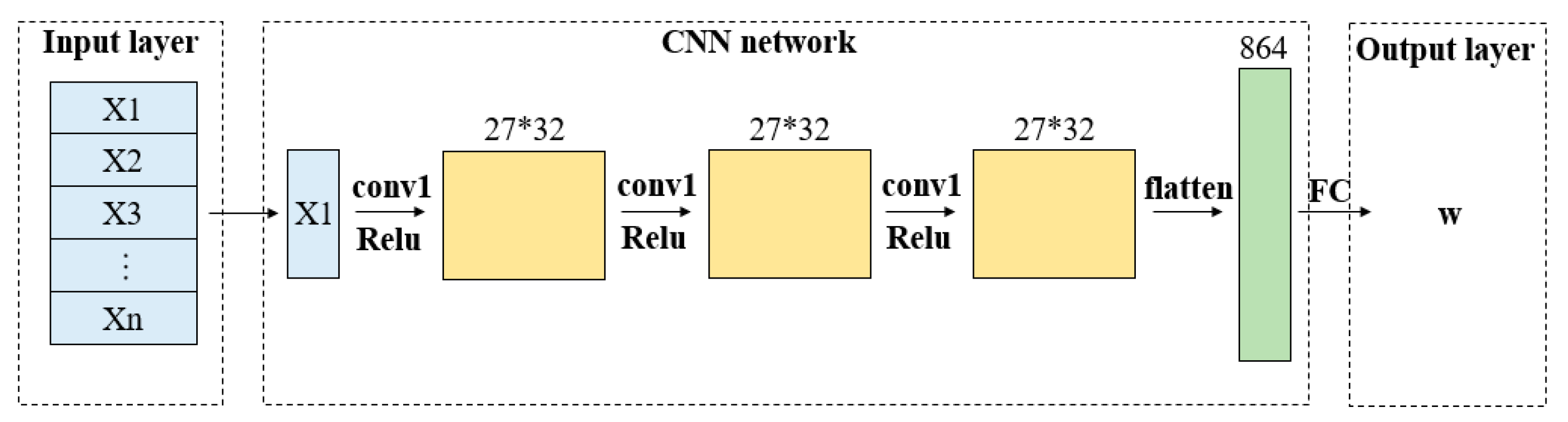
2.2.3. CNN
A CNN is a feed-forward neural network that performs well on image, audio, and text data. It is easy to update the data model by a back propagation algorithm. The CNN architecture (i.e., the number of layers and their structure) can be applied to a wide range of problems, while the hidden layers also reduce the algorithm’s reliance on feature engineering. A CNN is suitable for training with large amounts of data and is capable of solving complex nonlinear problems. The complete neural network structure includes input layer, convolution layer, Relu activation function, pooling layer, fully connected layer, and output layer [19,31]. The optimizer uses adaptive moment estimation (Adam) gradient descent algorithm instead of stochastic gradient descent (SGD) because Adam is able to adjust the learning rate of each parameter, making the parameters smooth for extracting data features. A total of Xn samples are trained and the inversed wind speed values W are output.
After a large amount of data validation, this paper finally determined the number of convolutional layers to be 3, no pooling layer was set, the convolutional kernel size was 3 × 1, dropout was 0.3, the number of convolutional kernels in each layer was 32, batch-size was 1000, and epochs were 2000. Figure 2 shows the structure of the CNN model used in this paper.
2.3. High Wind Speed Inversion Process
2.3.1. Data Processing Flow
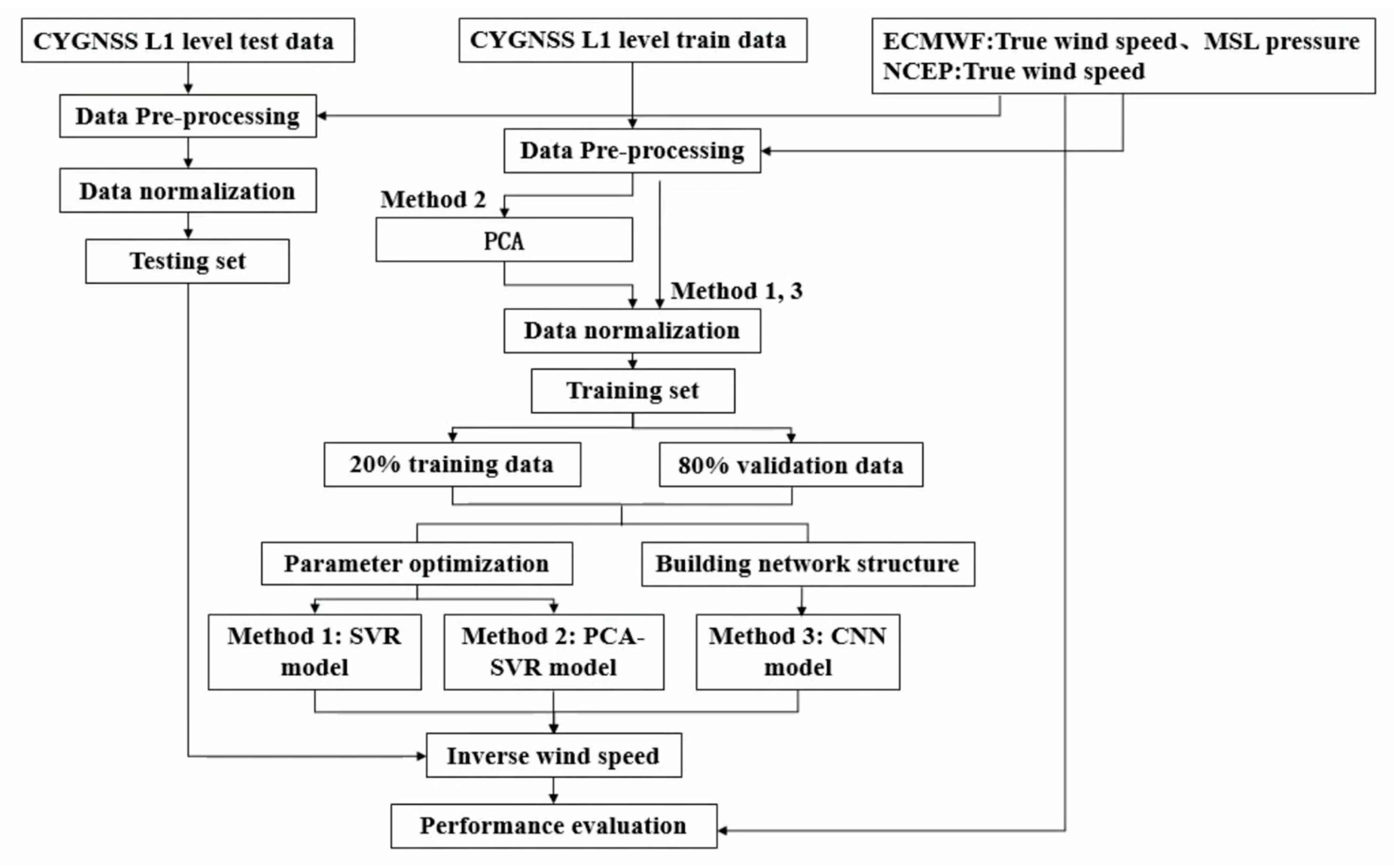
The process of high wind speed inversion in this paper can be briefly summarized into four parts: (i) determining the satellite data as well as wind speed data used; (ii) preprocessing and normalizing data; (iii) training the processed data with the three machine learning methods described above; (iv) using test data to inverse wind speed and analyzing performance of inversion wind speed. The specific wind speed inversion process is shown in Figure 3.
2.3.2. Data Pre-Processing
In order to obtain good results, any data derived from a remote sensing satellite for Earth observation needs to undergo rigorous data pre-processing. The datasets were processed according to the following criteria:
- (1)
- CYGNSS data quality control (QC) flags.
- (2)
- Positive values for both CYGNSS observations and wind speed matching data.
- (3)
- The RCG of the observations is greater than 10, with the RCG defined and described in [7].
- (4)
- The incidence angle of the satellite antenna is less than 60°.
- (5)
- The specular reflection point is at sea.
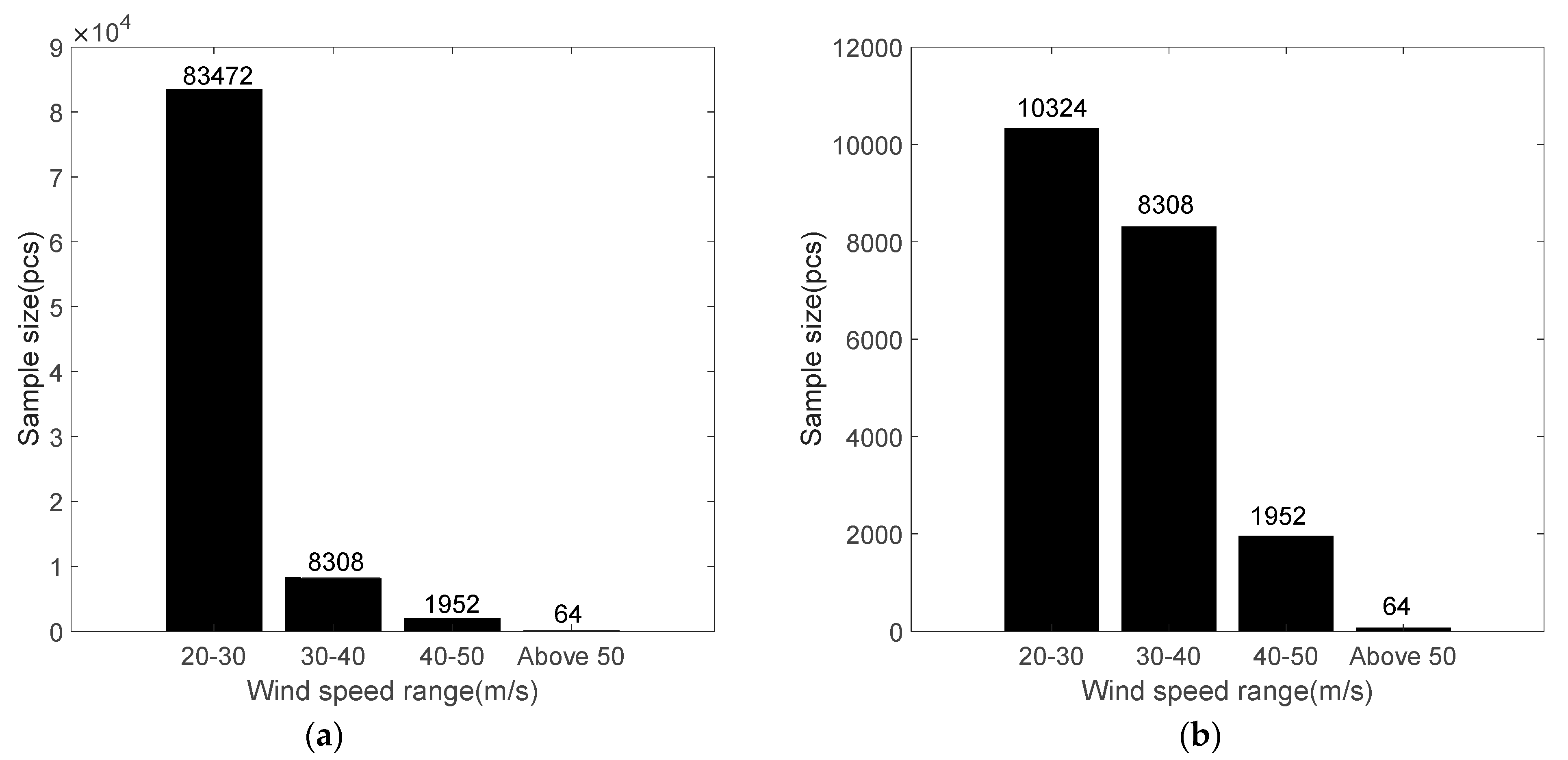
Because the occurrence time of each typhoon was not continuous, the CYGNSS data used in this paper was intermittent in time. CYGNSS data from 30 June 2018 to 3 July, 27 September 2018 to 30 September, 1 January 2019 to 3 January, 3 August 2019 to 8 August, 6 October 2019 to 12 October, 24 October 2019 to 25 October, 30 October 2019, 4 November 2019 to 7 November, 2 August 2020 to 4 August, 10 August 2020 to 11 August and 3 September 2020 were used as the train data (Figure 3), and the reanalysis wind speed datasets of ECMWF and NCEP in the corresponding time were used as the true wind speed data (Figure 3). Figure 4a,b respectively show the number of original samples and the corresponding number of final training samples for each wind speed range. The number of original samples means the data number after filtering the data according to the preprocessing criteria, and the number of final training samples means the training set data (including training data and validation data) number for Machine Leaning after under-sampling original samples.
From Figure 4a, we can see that the wind speed samples were concentrated between 20~30 m/s, the number of wind speed samples larger than 30 m/s and 20~30 m/s was seriously unbalanced, the imbalance of the number of samples easily led to the bias of the trained model, which did not have generalization. Therefore, the under-sampling method was used for random sampling to remove some majority samples from the training set, and in order to ensure that there were enough samples for training and that the amount of data for each type of wind speed interval was similar. Finally, when the ratio of samples between 20~30 m/s interval and more than 30 m/s interval was 1:1, a total of 20,648 final training samples were used for training. The specific samples are shown in Figure 4b. Subsequent model training and data research were based on this basis.
2.3.3. Feature Parameter Selection
After data pre-processing, it could be found that the L1 level data products of CYGNSS included many satellite observables, such as DDMA, LES, etc., which are characteristic values depending on wind speed as well as sea surface roughness. Due to the high wind speed measurement environment, especially typhoons, the sensitivity of the characteristic parameters of the two-dimensional delay-Doppler power waveform of the GNSS reflection signal to wind speed decreases, causing an increase in the wind speed measurement error. To reduce the performance error of CYGNSS in detecting typhoons, more characteristic parameters of CYGNSS L1 datasets were extracted to optimize the accuracy of the wind measurement model.
In this paper, 27 eigenvalues related to sea surface wind speed were used, specifically: Pseudo Random Noise (PRN) satellite number, DDMA, LES, antenna gain, distance from transmitter to specular reflection point, distance from receiver to specular reflection point, specular reflection point (longitude, latitude, time, and elevation angle), QC Flag, Signal-to-Noise Ratio (SNR), GNSS-R satellite position in ECEF, GNSS satellite position in ECEF, BRCS’s DDM (specular delay line and Doppler column), BRCS’s DDM (peak delay line and peak Doppler column), vehicle’s specular delay, corrected DDM instrument specular delay, the direct signal code phase, and MSL pressure.
3. Results and Discussion
3.1. Typhoon Validation Data
To analyze the feasibility of the three methods for wind speed inversion, the data of the Typhoon Bavi event in August 2020 were studied here. The reflected signal data collected by CYGNSS during Typhoon Bavi in the western Pacific Ocean during 2020.8.22~2020.8.26 were processed as test data (Figure 3). The reanalysis typhoon data released by ECMWF and NCEP were used as the true wind speed for the evaluation of wind measurement accuracy. Only wind speed data above 20 m/s during Typhoon Bavi were inversed here, because the training set in the Machine Learning method only includes data samples with wind speed greater than 20 m/s, as shown in Figure 4. A total of 7389 samples were available for the experiment over the four days. This subsection provides a detailed analysis of the CYGNSS satellite flight tracks and the corresponding true wind speeds during Typhoon Bavi.
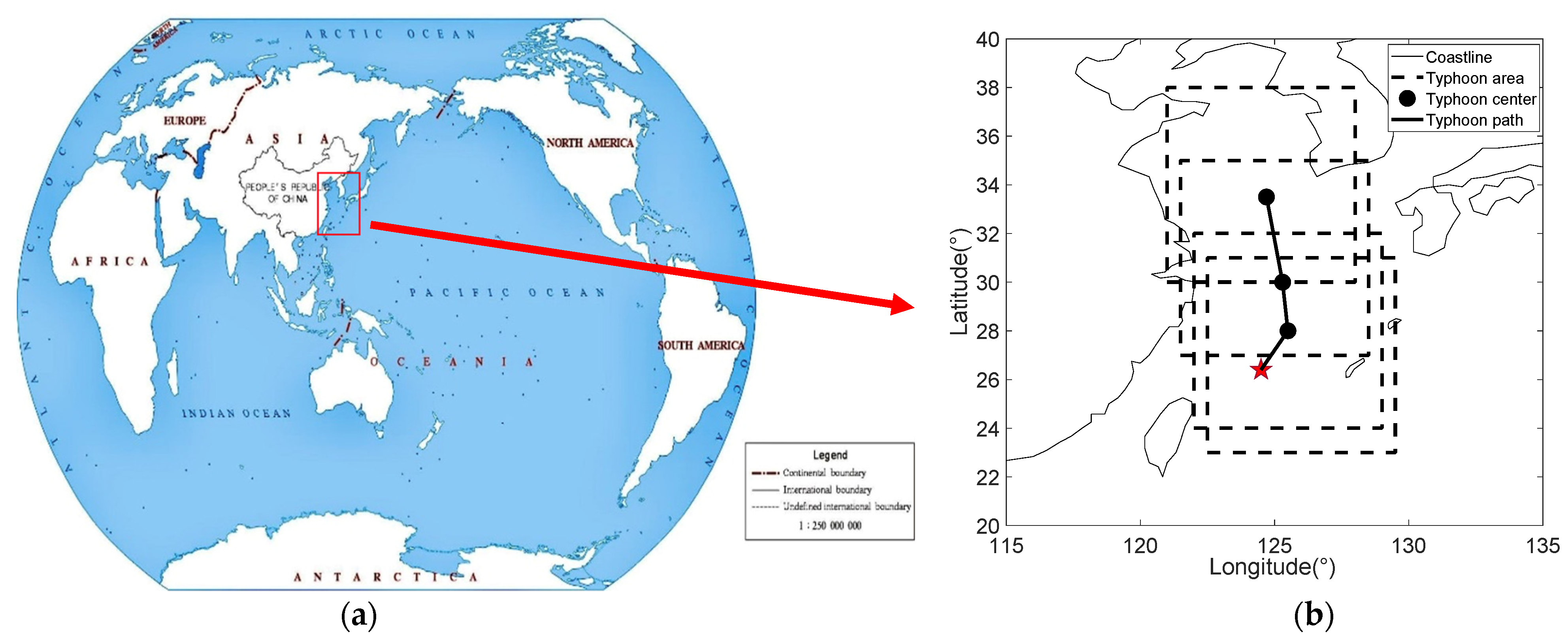
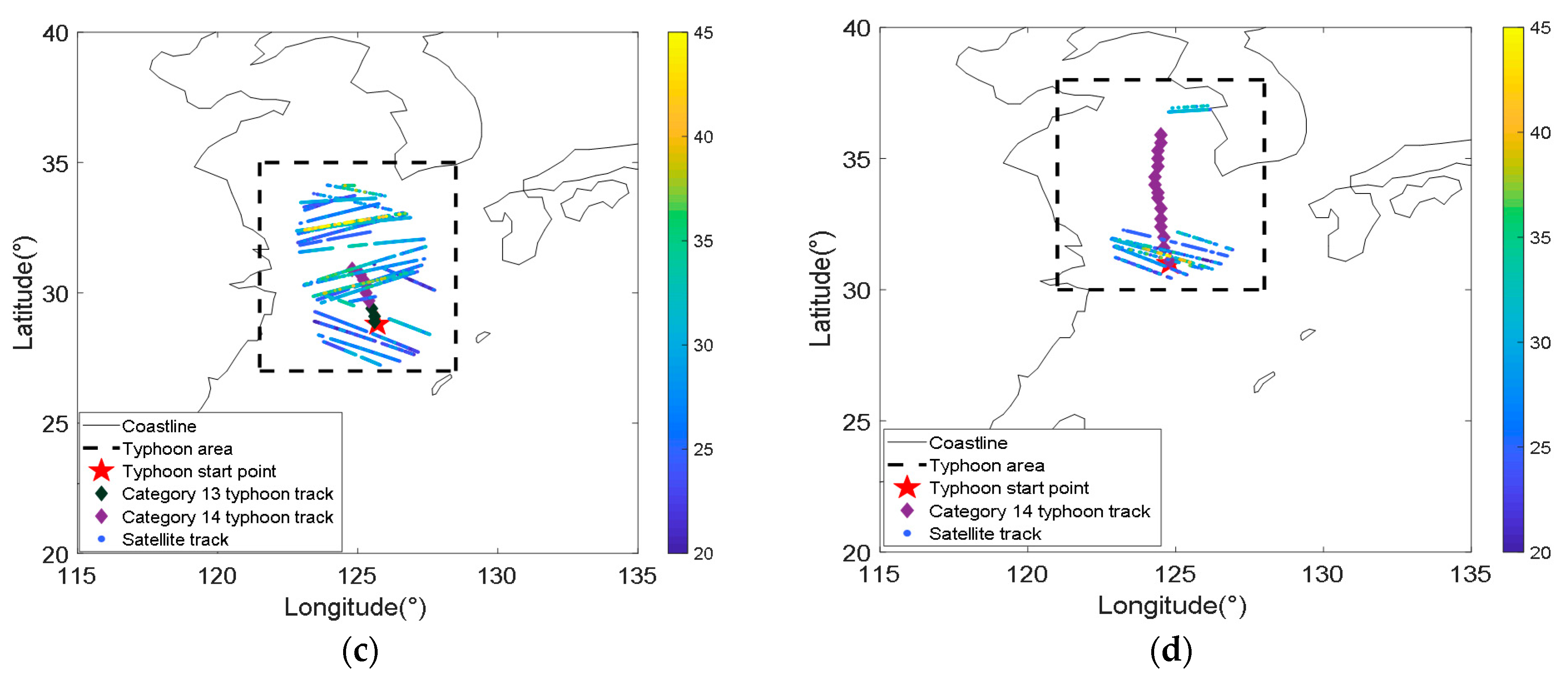
Figure 5a shows the location of region for performance evaluation, and Figure 5b shows Typhoon Bavi (2020.8.22~2020.8.26) moving track map and daily area of interest. The CYGNSS data during 2020.8.22~2020.8.26 was first preprocessed for data, and then analyzed specifically according to time after obtaining analyzable data. Typhoon Bavi occurred in the western Pacific Ocean. The typhoon hourly track data used in this study was collected by Department of Water Resources of Zhejiang Province (http://typhoon.zjwater.gov.cn/, accessed on 20 June 2021). In addition, it was combined with the data distribution of CYGNSS to determine the specific typhoon area. Since there was no data in the region after preprocessing on 22 August 2020, this paper mainly studied the data from 23 August 2020 to 26 August 2020. In Figure 5b, the five pointed star represents the starting position of the typhoon, and the dotted box represents each divided typhoon area. Table 1 shows the specific selection range of each regional division.
This paper mainly focused on the data with wind speed above 20 m/s. The proportion of samples has been determined in Section 2.3.2. Two measurement standards were used to compare the performance of three models: 1. Mean absolute error (MAE); 2. Root Mean Square Error (RMSE); and 3. Correlation Coefficient.
3.2. Analysis of Overall Inversion Results
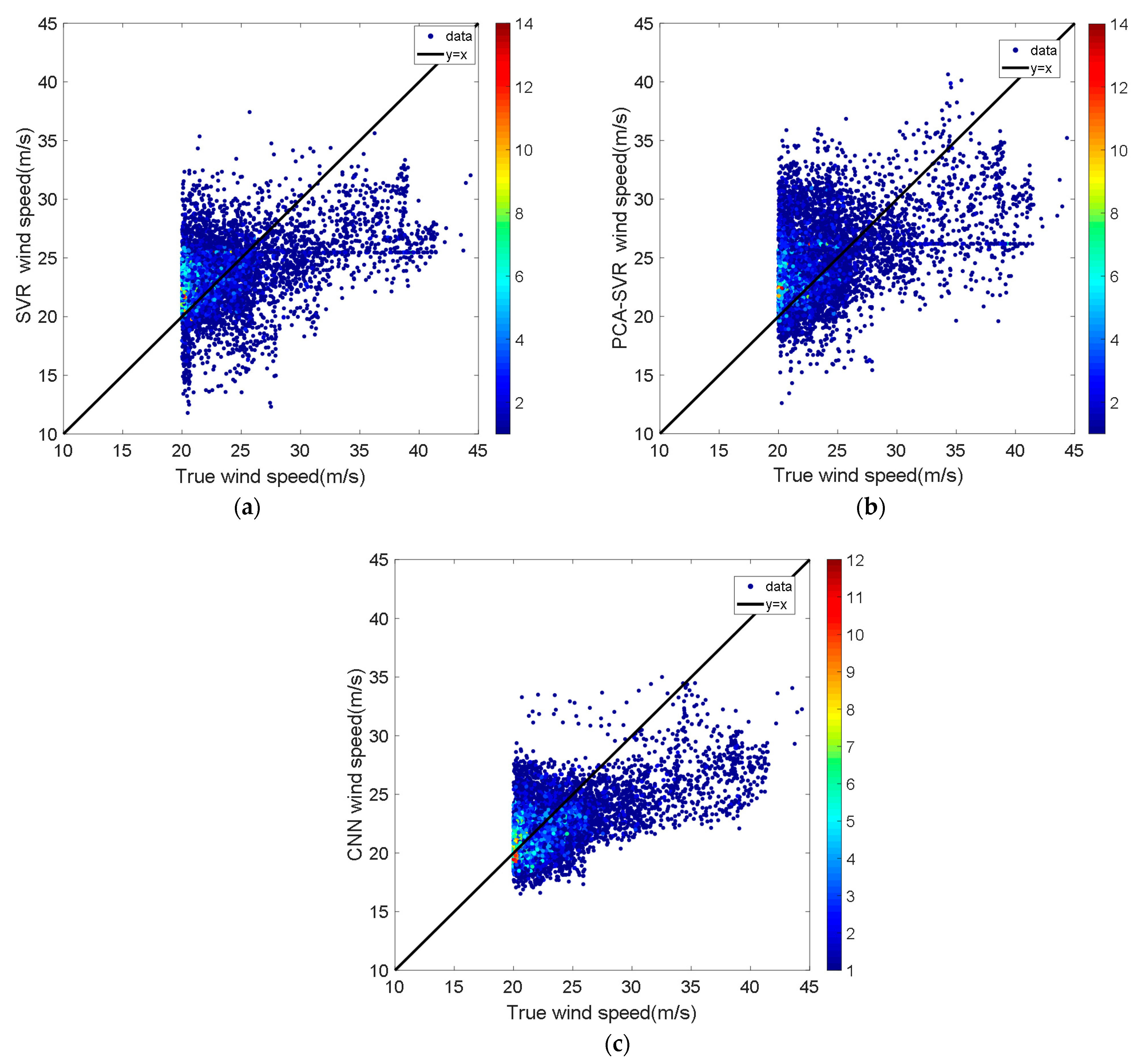
The overall performance of the three trained models was investigated for all data during the typhoon, and Figure 6 shows the scatter plots of the true and inverse wind speed for all data during the typhoon for the three models. Table 2 shows the specific performance analysis of the three models.
Firstly, it can be demonstrated from the scatter plot in Figure 6 that all three methods could be used to inverse the wind speed. In Figure 6, it was obvious that the SVR model inversion results had the greatest dispersion, and the inversion results reached a minimum of 10 m/s. The PCA-SVR model after adding data downscaling was partially improved for the problem of data divergence, but there was still a bias. The true wind speed of 20 m/s inversed the results around 35 m/s. While the CNN model had the most concentrated scattered data, the minimum inverse wind speed was about 15 m/s. The inversion results for the wind speed dataset around 20 m/s converged significantly and the outcomes were better than the other two methods. In general, the CNN method showed good inversion performance.
The performance of each of the three models was analyzed in three data intervals: (i) overall; (ii) 20~30 m/s; and (iii) above 30 m/s. From Table 2, except for the MAE value of CNN above 30 m/s, which was slightly inferior to SVR, all the error results indicated that CNN had the best performance. PCA-SVR was the second and SVR was the worst. Especially in the three data intervals, the correlation coefficients of CNN model were the highest. Further analysis showed that the MAE of CNN in the overall interval was improved by 33.90%, RMSE by 30.66% and correlation coefficient by 37.50% over SVR.
However, when the typhoon wind speed was greater than 30 m/s, the deviations of the wind speed values obtained from all three model inversions were all large, possibly because of the lack of higher wind speed train data (>40 m/s), as in Figure 4b, which leads to large bias in the inversion of typhoon data higher than 30 m/s.
3.3. Analysis of Daily Inversion Results by CNN Models
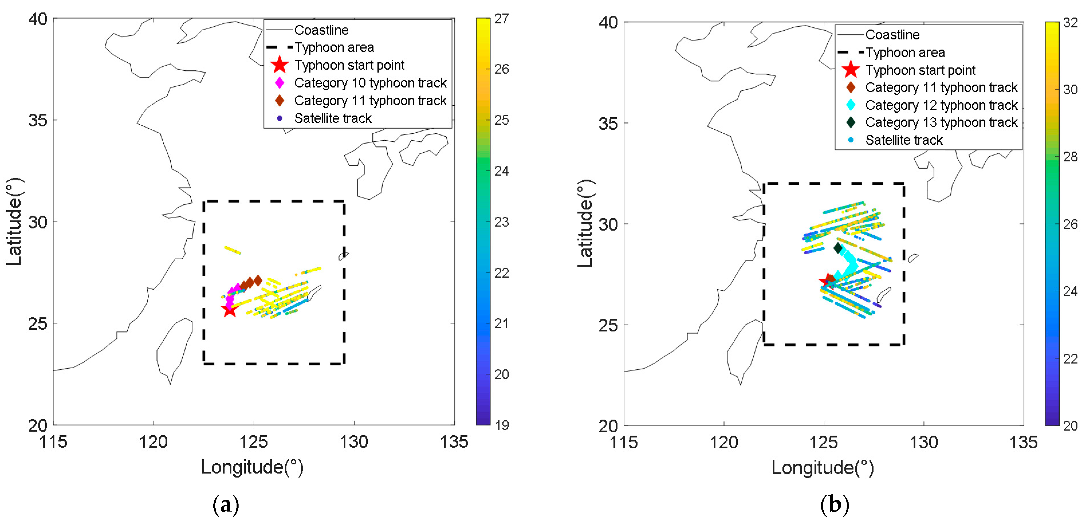
It was known from the analysis in Section 3.2 that the CNN model produced better wind speed inversion results for the overall data during typhoons. Considering the large variation of daily climatic environment and other factors during typhoons, which may affect the results of daily data collection from satellites for the same sea area, the CNN model was used for specific analysis of daily data. Figure 7 shows the daily CYGNSS satellite flight track and corresponding CNN wind speed, while Figure 8 corresponds to the absolute value of wind speed inversion (daily true wind speed minus the CNN model inverse wind speed). Table 3 shows the daily data performance results of the CNN model.
It can be seen from Figure 7 that the CNN model could be used to inverse the typhoon wind speed, and the inverse wind speed can reach up to 55 m/s. Figure 8 and Table 3 show that the inversion results for 23 and 24 August 2020 were smaller errors compared to the last two days. The reason was that the true wind speeds of the first two days were mostly less than 30 m/s. The true wind speed of the data on 25 and 26 August 2020 was up to 45 m/s, and there were more data in the interval of 30 m/s to 45 m/s, so the CNN inversion results showed relatively large errors. This conclusion coincides with the results in Table 2.
The above contents have verified the accuracy of the model. Next, the comparison between the inverse wind speed and the typhoon track data was discussed. Table 4 shows the results of the comparison between CNN inverse wind speed, true wind speed (ECMWF and NCEP reanalysis wind speed data), and Beaufort scale of typhoon track data (from Department of Water Resources of Zhejiang Province). The approximate wind speed is similar to Best Track data. The CYGNSS samples here should meet less than spatial ± 0.5° and temporal ± 0.5 h from the typhoon track data. The five datasets satisfied the above conditions.
In Table 4, comparing with CNN wind speed and Typhoon track data, the first column result had the smallest deviation, and the fifth column result was the worst. It shows the greater wind speed level, the worse error is obtained. It is the same result as Table 2 and Table 3, the reason has been analyzed before. However, in this paper, the true wind speed (ECMWF and NCEP reanalysis wind speed data) was used as the training benchmark of CNN model. As can be seen from Table 4, compared with the approximate wind speed (from Department of Water Resources of Zhejiang Province) during the typhoon, the true wind speed was actually underestimated, and the inversion performance of CNN model was limited by the true wind speed.
4. Conclusions
In response to the limitations of environmental conditions during typhoons, the high cost of collecting typhoon wind speed data leads to difficulties in obtaining training samples for high wind speeds. DDM observables such as DDMA and LES can change with the change of wind speed. Some traditional sea surface high wind speed inversion methods use a single DDM-derived observable (DDMA or LES), the incidence angle of specular reflection, and the significant wave height as parameters to establish GMF models with wind speed for wind speed inversion, which cannot fully explore the hidden features in the data. This limits the accuracy of high wind speed inversion. In order to use multi-dimensional data features to fully exploit the data during typhoons and improve the accuracy of the inversion of typhoon wind speeds in the sea area and the performance of real-time monitoring, this paper proposed a CYGNSS inversion method for high wind speed on the sea surface based on machine learning. Firstly, CYGNSS satellite data and true wind speed data from ECMWF and NCEP were used to construct the original datasets, and then three machine learning methods, SVR, PCA-SVR, and CNN, were used to train the data greater than 20 m/s during the typhoon. To avoid bias of the models, the under-sampling method was adopted to control the number of samples. Lastly, the trained models were used for the inversion of Typhoon Bavi from 23 to 26 August 2020. The following conclusions could be drawn from the experimental results.
- (1)
- All three models can be used to inverse the sea surface high wind speed from CYGNSS data. SVR can effectively solve the regression problem of high-dimensional characteristics, so the 27-dimensional characteristic parameters can be finally regressed to the wind speed value. Due to the large samples and high mapping dimension of kernel function, the calculation is too large, so PCA is used to reduce the dimension of data, which can speed up the training speed and obtain better wind speed inversion results.
- (2)
- The CNN method can map arbitrarily complex nonlinear relationships and extract hidden deep-level features in the data. Even better, it also has the characteristics of strong robustness and self-learning capability. From an overall perspective, better results were obtained by using the CNN model for sea surface high wind speed inversion. The MAE of CNN was 2.71 m/s and RMSE was 3.8 m/s. Compared with the SVR model, the MAE of CNN was improved by 33.90% and RMSE improved by 30.66%. However, the inversion results of the three models for wind speeds above 30 m/s had large deviations. The reason for this error may be related to the lack of high wind speed data.
- (3)
- The daily data inversion results during the typhoon show that CNN can be applied to the high wind speed inversion when the daily climate environment and other factors change greatly during the typhoon. Compared with the wind speed data at the typhoon center point provided by the Department of Water Resources of Zhejiang Province, it can be found that the higher the wind level, the larger the error between the true wind speed and the CNN inversion wind speed value near the typhoon center point. This error was caused by using underestimated true wind speeds (ECMWF and NCEP reanalysis wind speed data) to train the CNN model.
The difficulty of high wind speed inversion is the lack of higher wind speed samples, especially more than 40 m/s data, which leads to insufficient model training. Except for this, the selection of true wind speed during typhoons for training is also the key to the performance of the inversion. In the future, with the increasing amount of higher wind speed data and the use of more accurate model winds such as HWRF, GPS Dropsondes, and SFMR during typhoons, the accuracy of the obtained model will be improved and the error of typhoon inversion will be reduced. Eventually, the real-time prediction capability of typhoons will be realized.
Author Contributions
Y.Z. and Y.H. conceived and designed the framework of the study. J.Y. completed the data collection and processing. Y.Z. and J.Y. completed the algorithm design and the data analysis and were the lead authors of the manuscript, with contributions from J.Y., W.M., Z.Y. and S.Y. All authors have read and agreed to the published version of the manuscript.
Funding
This work was supported by the National Natural Science Foundation of China (Grant No. 41871325) and the National Key R&D Program of China (Project No. 2019YFD0900805).
Institutional Review Board Statement
Not applicable.
Informed Consent Statement
Not applicable.
Data Availability Statement
The raw/processed data required to reproduce these findings cannot be shared at this time as the data also forms part of an ongoing study.
Acknowledgments
Thanks NASA for the CYGNSSS public data; the European Centre for Medium-Range Weather Forecasts (ECMWF) and the National Centers for Environmental Prediction (NCEP) for the reanalysis dataset; and Department of Water Resources of Zhejiang Province for the typhoon track data. We would also like to thank Professor Yang Dongkai of Beijing University of Aeronautics and Astronautics and Li Weiqiang of CSIC-IEEC for their suggestions on GNSS-R satellite data analysis. We would like to thank Zhou Bo and Qin Jin from Shanghai Institute of Aerospace Electronics for their suggestions on the receiver of reflected signals.
Conflicts of Interest
The authors declare no conflict of interest.
References
- Lin, M.; Sun, Y.; Zhen, S. Study on the inversion method of ocean wind field measurement by satellite-borne microwave scatterometer. Acta Oceanol. Sin. 1997, 5, 35–46. [Google Scholar]
- Wang, Z.; Jiang, J.; Liu, J. Key technologies and scientific aspects of remote sensing of sea surface wind fields by all-polarization microwave radiometer. Strateg. Stud. CAE 2008, 10, 76–86. [Google Scholar] [CrossRef]
- Zhang, W.; Shi, H.; Jiang, Z.; Yang, P.; Chang, S.; Xiang, J. Evaluation of variational scheme for synthetic aperture radar wind field inversion. Chin. J. Geophys. 2021, 64, 2436–2446. [Google Scholar] [CrossRef]
- Hasager, C.B.; Hahmann, A.N.; Ahsbahs, T.; Karagali, I.; Sile, T.; Badger, M.; Mann, J. Europe’s offshore winds assessed with synthetic aperture radar, ASCAT and WRF. Wind Energy Sci. 2020, 5, 375–390. [Google Scholar] [CrossRef] [Green Version]
- Kilic, L.; Prigent, C.; Boutin, J.; Meissner, T.; English, S.; Yueh, S. Comparisons of Ocean Radiative Transfer Models With SMAP and AMSR2 Observations. J. Geophys. Res. Oceans 2019, 124, 7683–7699. [Google Scholar] [CrossRef]
- Clarizia, M.; Ruf, C.; Jales, P. Spaceborne GNSS-R Minimum Variance Wind Speed Estimator. IEEE Trans. Geosci. Remote Sens. 2014, 52, 6829–6843. [Google Scholar] [CrossRef]
- Clarizia, M.; Ruf, C. Wind Speed Retrieval Algorithm for the Cyclone Global Navigation Satellite System (CYGNSS) Mission. IEEE Trans. Geosci. Remote Sens. 2016, 58, 4419–4432. [Google Scholar] [CrossRef]
- Wang, F.; Yang, D.; Zhang, B.; Li, W. Waveform-based spaceborne GNSS-R wind speed observation: Demonstration and analysis using UK TechDemoSat-1 data. ADV Space Res. 2018, 61, 1573–1587. [Google Scholar] [CrossRef]
- Ruf, C.; Balasubramaniam, R. Development of the CYGNSS Geophysical Model Function for Wind Speed. IEEE J-STARS 2018, 12, 66–77. [Google Scholar] [CrossRef]
- Reynolds, J.; Clarizia, M.; Santi, E. Wind Speed Estimation from CYGNSS Using Artificial Neural Networks. IEEE J-STARS 2020, 13, 708–716. [Google Scholar] [CrossRef]
- Yang, D.; Liu, Y.; Wang, F. Research on the inversion method of satellite-based GNSS-R sea surface wind speed. J. Electron. Inform. Technol. 2018, 40, 462–469. [Google Scholar] [CrossRef]
- Ruf, C.; Asharaf, S.; Balasubramaniam, R.; Gleason, S.; Lang, T.; McKague, D.; Twigg, D.; Waliser, D. InOrbit Performance of the Constellation of CYGNSS Hurricane Satellites. Bull. Am. Meteorol. Soc. 2019. [Google Scholar] [CrossRef]
- Rodriguez-Alvarez, N.; Garrison, J. Generalized Linear Observables for Ocean Wind Retrieval From Calibrated GNSS-R Delay–Doppler Maps. IEEE Trans. Geosci. Remote 2016, 54, 1142–1155. [Google Scholar] [CrossRef]
- Said, F.; Katzberg, S.; Soisuvarn, S. Retrieving Hurricane Maximum Winds Using Simulated CYGNSS Power-Versus-Delay Waveforms. IEEE J-STARS 2017, 10, 3799–3809. [Google Scholar] [CrossRef]
- Al-Khaldi, M.; Johnson, J.; Kang, Y.; Steven, J. Track-Based Cyclone Maximum Wind Retrievals Using the Cyclone Global Navigation Satellite System (CYGNSS) Mission Full DDMs. IEEE J-STARS 2019, 13, 21–29. [Google Scholar] [CrossRef]
- Al-Khaldi, M.; Katzberg, S.J.; Johnson, J. Matched Filter Cyclone Maximum Wind Retrievals Using CYGNSS: Progress Update and Error Analysis. IEEE J-STARS 2021, 99, 3591–3601. [Google Scholar] [CrossRef]
- Wu, C.; Yan, S.; Yang, Y.; Bu, F.; Chen, Z. An inversion method for ocean surface wind speed based on time-lapse-Doppler images. Bull. Sci. Technol. 2019, 35, 22–30. [Google Scholar] [CrossRef]
- Gao, H.; Bai, Z.; Fan, D. GNSS-R sea surface wind speed inversion based on BP neural network. Chin. J. Aeronaut 2019, 40, 198–206. [Google Scholar] [CrossRef]
- Wang, S. Research on GNSS-R Sea Surface Wind Speed Inversion Algorithm Based on Neural Network Model. Master’s Thesis, University of Chinese Academy of Sciences, Beijing, China, 2020. [Google Scholar] [CrossRef]
- Cardellach, E.; Nan, Y.; Li, W. Variational Retrievals of High Winds Using Uncalibrated CyGNSS Observables. Remote Sens. 2020, 12, 3930. [Google Scholar] [CrossRef]
- Saïd, F.; Jelenak, Z.; Park, J.; Chang, P. The NOAA Track-Wise Wind Retrieval Algorithm and Product Assessment for CyGNSS. IEEE Trans. Geosci. Remote Sens. 2021, 1–24. [Google Scholar] [CrossRef]
- Shao, L.; Zhou, X.; Zhang, C.; Liu, H. Analysis of satellite-based GNSS-R typhoon observations. Remote Sens. Inf. 2020, 4, 35–39. [Google Scholar]
- Gong, W.; Shi, C.; Zhang, T.; Meng, X. Evaluation of mean sea level pressure and surface wind speed from two numerical models in China. J. Glaciol. Geocryol. 2015, 37, 1497–1507. [Google Scholar] [CrossRef]
- Hou, M.; Wang, G.; Bu, Q. Analysis of wind speed characteristics based on four reanalysis data offshore China. Tianjin Sci. Technol. 2017, 44, 109–113. [Google Scholar] [CrossRef]
- Pan, Y.; Xu, J.; Zhang, Y.; Yuan, S.; Zhu, W. Simulation of the 2015 Northwest Pacific tropical cyclone based on the East Asian regional reanalysis system. J. Zhanjiang Ocean Univ. 2020, 40, 53–63. [Google Scholar]
- Saini, J.; Dutta, M.; Marques, G. Fuzzy Inference System Tree with Particle Swarm Optimization and Genetic Algorithm: A novel approach for PM10 forecasting. Syst. Appl. 2021, 183, 115376. [Google Scholar] [CrossRef]
- Bergadano, F.; Raedt, L. Machine Learning: ECML-94 Volume 784|| Estimating attributes: Analysis and extensions of RELIEF. LNCS 1997, 11, 171–182. [Google Scholar] [CrossRef] [Green Version]
- Last, M. Kernel Methods for Pattern Analysis. J. Am. Stat. Assoc. 2006, 101, 1730. [Google Scholar] [CrossRef]
- Alex, J.; Bernhard, S. A tutorial on support vector regression. Stat. Comput. 2004, 14, 199–222. [Google Scholar] [CrossRef] [Green Version]
- Liu, B.; Qi, X. Research on prediction of industrial solid waste generation in China based on PCA-SVR model. J. Henan Normal Univ. 2020, 48, 69–74. [Google Scholar] [CrossRef]
- Ma, Q.; Zhang, X.; Zhang, C.; Zhou, H.; Wu, Z. Cross-wave velocity prediction based on one-dimensional convolutional neural network. Lith Res. 2021, 1–10. Available online: http://kns.cnki.net/kcms/detail/62.1195.TE.20210530.1549.002.html (accessed on 5 June 2021).
Figure 1.
PCA-SVR model structure.

Figure 2.
CNN model structure (Conv: Convolution layer, FC: fully connected layer).

Figure 3.
High wind speed inversion process based on machine learning.

Figure 4.
(a) Original training samples histogram; (b) Final training samples histogram.

Figure 5.
(a) Location of the region for performance evaluation (world map: preview number: GS (2016) 1563); (b) Typhoon Bavi (2020.8.22~2020.8.26) moving track map and daily interested area.
Figure 5.
(a) Location of the region for performance evaluation (world map: preview number: GS (2016) 1563); (b) Typhoon Bavi (2020.8.22~2020.8.26) moving track map and daily interested area.

Figure 6.
(a) SVR model wind speed inversion results; (b) PCA-SVR model wind speed inversion results; and (c) CNN model wind speed inversion results. The color bar on the right represents data density.
Figure 6.
(a) SVR model wind speed inversion results; (b) PCA-SVR model wind speed inversion results; and (c) CNN model wind speed inversion results. The color bar on the right represents data density.

Figure 7.
(a) 2020.8.23 CYGNSS satellite flight track and corresponding CNN wind speed; (b) 2020.8.24 CYGNSS satellite flight track and corresponding CNN wind speed; (c) 2020.8.25 CYGNSS satellite flight track and corresponding CNN wind speed; (d) 2020.8.25 CYGNSS satellite flight track and corresponding CNN wind speed. The color bar on the right represents the wind speed value, Unit: m/s.


Figure 8.
(a) 2020.8.23 CYGNSS satellite flight track and corresponding inversion error; (b) 2020.8.24 CYGNSS satellite flight track and corresponding inversion error; (c) 2020.8.25 CYGNSS satellite flight track and corresponding inversion error; (d) 2020.8.26 CYGNSS satellite flight track and corresponding inversion error. The color bar on the right represents the wind speed value, Unit: m/s.


Table 1.
2020.8.22~2020.8.26 typhoon area latitude and longitude selection range.
| Date | Longitude Range (°) | Latitude Range (°) |
|---|---|---|
| 8.22 | 120°~127° | 22°~30° |
| 8.23 | 122.5°~129.5° | 23°~31° |
| 8.24 | 122°~129° | 24°~32° |
| 8.25 | 121.5°~128.5° | 27°~35° |
| 8.26 | 121°~128° | 30°~38° |
Table 2.
Model performance analysis (Correl. Coef. represents the correlation coefficient).
| Performance (m/s) | Overall Interval | 20~30 m/s | Above 30 m/s | ||||||
|---|---|---|---|---|---|---|---|---|---|
| SVR | PCA-SVR | CNN | SVR | PCA-SVR | CNN | SVR | PCA-SVR | CNN | |
| MAE | 4.10 | 3.85 | 2.71 | 3.66 | 3.32 | 2.10 | 8.44 | 9.08 | 8.52 |
| RMSE | 5.48 | 5.10 | 3.80 | 4.88 | 4.17 | 2.64 | 9.51 | 10.50 | 9.22 |
| Correl. Coef. | 0.40 | 0.41 | 0.55 | 0.20 | 0.24 | 0.25 | 0.28 | 0.19 | 0.32 |
Table 3.
CNN model daily data performance analysis results.
| Date | Aug. 23 | Aug. 24 | Aug. 25 | Aug. 26 |
|---|---|---|---|---|
| MAE (m/s) | 2.33 | 2.29 | 4.18 | 4.21 |
| RMSE (m/s) | 2.95 | 2.92 | 5.70 | 5.25 |
Table 4.
Comparison results of wind speed data from Department of Water Resources of Zhejiang Province.
Table 4.
Comparison results of wind speed data from Department of Water Resources of Zhejiang Province.
| Beaufort Scale (Approximate Wind Speed) | 11 (30 m/s) | 12 (33 m/s) | 12 (38 m/s) | 14 (42 m/s) | 14 (42 m/s) |
|---|---|---|---|---|---|
| Date | Aug. 24 | Aug. 24 | Aug. 25 | Aug. 25 | Aug. 26 |
| True wind speed (m/s) | 20.07 | 20.01 | 24.99 | 33.66 | 34.00 |
| CNN wind speed (m/s) | 19.24 | 22.88 | 27.47 | 28.94 | 24.78 |
| Distance from the center of the typhoon track (km) | 56.54 | 26.03 | 57.60 | 50.91 | 66.91 |
Publisher’s Note: MDPI stays neutral with regard to jurisdictional claims in published maps and institutional affiliations. |
© 2021 by the authors. Licensee MDPI, Basel, Switzerland. This article is an open access article distributed under the terms and conditions of the Creative Commons Attribution (CC BY) license (https://creativecommons.org/licenses/by/4.0/).
Share and Cite
MDPI and ACS Style
Zhang, Y.; Yin, J.; Yang, S.; Meng, W.; Han, Y.; Yan, Z. High Wind Speed Inversion Model of CYGNSS Sea Surface Data Based on Machine Learning. Remote Sens. 2021, 13, 3324. https://0-doi-org.brum.beds.ac.uk/10.3390/rs13163324
AMA Style
Zhang Y, Yin J, Yang S, Meng W, Han Y, Yan Z. High Wind Speed Inversion Model of CYGNSS Sea Surface Data Based on Machine Learning. Remote Sensing. 2021; 13(16):3324. https://0-doi-org.brum.beds.ac.uk/10.3390/rs13163324
Chicago/Turabian StyleZhang, Yun, Jiwei Yin, Shuhu Yang, Wanting Meng, Yanling Han, and Ziyu Yan. 2021. "High Wind Speed Inversion Model of CYGNSS Sea Surface Data Based on Machine Learning" Remote Sensing 13, no. 16: 3324. https://0-doi-org.brum.beds.ac.uk/10.3390/rs13163324
Note that from the first issue of 2016, this journal uses article numbers instead of page numbers. See further details here.