Article

Comparative Evaluation of Algorithms for Leaf Area Index Estimation from Digital Hemispherical Photography through Virtual Forests

1
Key Laboratory of Virtual Geographic Environment (Nanjing Normal University), Ministry of Education, Nanjing 210023, China
2
Jiangsu Center for Collaborative Innovation in Geographical Information Resource Development and Application, Nanjing 210023, China
3
Mathematics, Unit of Computing Sciences, Tampere University, 33720 Tampere, Finland
4
Faculty of Geo-Information Science and Earth Observation (ITC), University of Twente, 7514 AE Enschede, The Netherlands
5
Department of Visitor Management and National Park Monitoring, Bavarian Forest National Park, 94481 Grafenau, Germany
6
Wildlife Ecology and Wildlife Management, University of Freiburg, 79098 Freiburg, Germany
*
Author to whom correspondence should be addressed.
Remote Sens. 2021, 13(16), 3325; https://0-doi-org.brum.beds.ac.uk/10.3390/rs13163325
Submission received: 11 June 2021 / Revised: 18 August 2021 / Accepted: 20 August 2021 / Published: 23 August 2021
(This article belongs to the Special Issue Virtual Forest)

Abstract

:
The in situ leaf area index (LAI) measurement plays a vital role in calibrating and validating satellite LAI products. Digital hemispherical photography (DHP) is a widely used in situ forest LAI measurement method. There have been many software programs encompassing a variety of algorithms to estimate LAI from DHP. However, there is no conclusive study for an accuracy comparison among them, due to the difficulty in acquiring forest LAI reference values. In this study, we aim to use virtual (i.e., computer-simulated) broadleaf forests for the accuracy assessment of LAI algorithms in commonly used LAI software programs. Three commonly used DHP programs, including Can_Eye, CIMES, and Hemisfer, were selected since they provide estimates of both effective LAI and true LAI. Individual tree models with and without leaves were first reconstructed based on terrestrial LiDAR point clouds. Various stands were then created from these models. A ray-tracing technique was combined with the virtual forests to model synthetic DHP, for both leaf-on and leaf-off conditions. Afterward, three programs were applied to estimate PAI from leaf-on DHP and the woody area index (WAI) from leaf-off DHP. Finally, by subtracting WAI from PAI, true LAI estimates from 37 different algorithms were achieved for evaluation. The performance of these algorithms was compared with pre-defined LAI and PAI values in the virtual forests. The results demonstrated that without correcting for the vegetation clumping effect, Can_Eye, CIMES, and Hemisfer could estimate effective PAI and effective LAI consistent with each other (R2 > 0.8, RMSD < 0.2). After correcting for the vegetation clumping effect, there was a large inconsistency. In general, Can_Eye more accurately estimated true LAI than CIMES and Hemisfer (with R2 = 0.88 > 0.72, 0.49; RMSE = 0.45 < 0.7, 0.94; nRMSE = 15.7% < 24.21%, 32.81%). There was a systematic underestimation of PAI and LAI using Hemisfer. The most accurate algorithm for estimating LAI was identified as the P57 algorithm in Can_Eye which used the 57.5° gap fraction inversion combined with the finite-length averaging clumping correction. These results demonstrated the inconsistency of LAI estimates from DHP using different algorithms. It highlights the importance and provides a reference for standardizing the algorithm protocol for in situ forest LAI measurement using DHP.

1. Introduction

The leaf area index (LAI), defined as one-half of the total green leaf area per unit horizontal ground surface area [1], is a key vegetation structural parameter influencing the process of photosynthesis, transpiration, and rain interception. Because of its importance, LAI has been identified as both an essential climate variable and an essential biodiversity variable [2,3]. In situ LAI measurement plays a vital role in monitoring vegetation dynamics from the ground, as well as for calibrating and validating satellite LAI products. Digital hemispherical photography (DHP) is widely used for in situ LAI measurement. It obtains photographs of the forest vegetation from the ground looking upward through a fisheye lens. By analyzing these photos, the gap fraction can be determined after separating the foliage from the sky, and LAI can be estimated using the gap fraction model. Compared to other techniques such as LAI-2200 and TRAC (tracing radiation and architecture of canopies), DHP has the advantages of lower costs, enhanced visual inspection of canopies, and a permanent archive that can be reprocessed when refined models become available [4]. DHP has been used for vegetation phenology studies [5,6]. DHP collected in the VALERI (Validation of Land European Remote sensing Instruments), and the NEON (National Ecological Observatory Network) was used to evaluate satellite LAI products [7,8,9,10]. LAI estimated from terrestrial [11], airborne [12,13], and spaceborne LiDAR [14] also relied on DHP for validation. Recent studies have pointed out the lack of long-term ground observation and suggested the expansion of existing in situ LAI observation networks as a “high priority” to enhance the quality of satellite-based LAI products [15,16].
There are several steps involved in the processing of DHP to estimate LAI, including the differentiation between sky pixels and canopy pixels, the calculation of gap fraction and gap size, the estimation of clumping index, and the estimation of LAI from gap fraction or gap size distribution inversion [17]. In forests, due to the existence of woody components such as tree trunks and branches, the plant area index (PAI) rather than LAI is estimated from DHP. Effective PAI (PAIeff) is derived from DHP, assuming that canopy elements are randomly distributed, while true PAI (PAItrue) is derived if the non-randomness of canopy elements is corrected through the estimation of the clumping index.
There are various LAI algorithms implemented in freely available programs to process DHP for PAI/LAI estimation. These algorithms mainly differ in how the PAI eff is estimated, how the orientation and the clumping of leaves are estimated, and how pure canopy segments with zero gap fraction are handled. Some widely used programs include Gap Light Analyzer (GLA) [18], Can_Eye [19], CIMES [4], and Hemisfer [20]. GLA has been continuously used for LAI estimation [5,21,22]. Nevertheless, GLA only provides estimates of PAIeff, as it does not correct for the clumping effect. Can_Eye, developed by the French National Institute of Agricultural Research, has been used extensively in previous studies [23,24,25,26,27]. Hemisfer, developed by the Swiss Federal Institute for the Forest, Snow, and Landscape Research, has been widely used as well [28,29,30]. CIMES is a package of programs encompassing various LAI retrieval methods and is particularly flexible for batch processing multiple DHP images [31,32,33]. Faced with these options, the question that often arises for users is which algorithm of which program produces more accurate LAI estimates. Addressing this problem can provide guidance for standardizing LAI estimation protocols and reducing in situ LAI measurement uncertainty.
Few studies have carried out the accuracy evaluation of different algorithms in commonly used DHP programs when estimating forest LAI. Glatthorn and Beckschäfer compared seven binarization algorithms to classify foliage and sky pixels and found that three algorithms (including Minimum, Edge Detection, and Minimum Histogram) achieved the highest accuracies. This analysis focused only on the gap fraction determination step [34]. Jarčuška et al. (2010) compared the consistency of GLA and WinSCANOPY and found that they produced similar PAIeff estimates [35]. The study by Promis et al. (2011) found similar PAIeff estimates from GLA and Winphot [36]. Similarly, Hall et al. (2017) found that Can_Eye and CIMES produced comparable PAIeff estimates. However, the two programs produced statistically significant different clumping index estimates and, thus, different PAItrue estimates [37]. It is worth noting that these studies only evaluated the consistency of results from different algorithms, instead of the accuracy of each algorithm, due to a lack of true reference values. A few studies have used destructive sampling or litterfall collection to acquire LAI reference values for validating the accuracy of DHP in LAI estimation [27,38,39]. However, there is no conclusive evidence concerning the accuracy comparison of various algorithms implemented in these different DHP programs. This calls for an accuracy assessment so that they can be used in the community with confidence.
Since the lack of LAI reference values is the main obstacle for DHP accuracy evaluation, virtual forests offer an alternative platform other than a destructive sampling of all leaves. Virtual forests are a relatively new area still under research. Some researchers define a virtual forest as a computer-based replica of the real forest which is assumed to be of interest for professional and non-professional forest users [40]. Virtual forests can be used for modeling forest growth, predicting forest fire spread, and enabling virtual tourism, as well as calibrating and validating remote sensing data in forest areas [41,42]. There are some previous studies utilizing virtual forests and synthetic DHP to validate the accuracy of the clumping index and PAItrue estimates [43,44], leaf angle distribution [45], and slope correction on estimating PAIeff [46]. Nevertheless, these studies used simple geometric primitives to model trees, which differ from real trees, especially in terms of the woody component structure. Recently, highly realistic tree models have been reconstructed from terrestrial LiDAR point clouds and further used to construct virtual forests [47]. Combined with a ray-tracing technique, synthetic DHP is generated for evaluating the retrieval of the clumping index [48]. More recently, Zou et al. (2018) used virtual forests to assess the performance of seven inversion models in estimating the PAI and LAI values from combined leaf-on and leaf-off DHP [49]. Some simulation studies use virtual isolated trees with realistic tree architecture to evaluate the accuracy of leaf area density and LAI estimation for individual trees [50,51]. To the best of our knowledge, there have been no conclusive studies with accuracy evaluations of algorithms implemented in commonly used DHP software programs. Virtual forests provide the potential to solve this problem.
In this study, our research objective is to use virtual broadleaf forests to assess and compare the accuracy of various algorithms implemented in three commonly used DHP software programs in estimating LAI. Both leaf-on and leaf-off virtual forests were created to assess the retrieval of the plant area index (PAI) and leaf area index (LAI). A total of 37 algorithms in three DHP programs, including Can_Eye, CIMES, and Hemisfer, were evaluated. Algorithms and software that do not correct for the clumping effect were not incorporated in the comparison. We aim to provide guidance for users and to identify future directions for the algorithm development of in situ LAI estimation using DHP.

2. Materials and Methods

The overall experimental design is displayed in Figure 1. Explicit individual tree models (quantitative structure models, QSM) with and without leaves were first constructed by tree reconstruction from point clouds and leaf insertion. Then, the trees were placed randomly to create a series of virtual forest stands with different stem densities and LAI. Synthetic DHP was simulated using a ray-tracing technique, for both leaf-on and leaf-off virtual forests. Afterward, 37 different algorithms utilized in three software packages, including Can_Eye, CIMES, and Hemisfer, were used to process the leaf-on DHP for plant area index (PAI) and leaf-off DHP for woody area index (WAI) estimation. The derived LAI estimates (via subtraction of WAI from PAI) were compared with pre-defined LAI reference values in the virtual forest stands for accuracy evaluation.

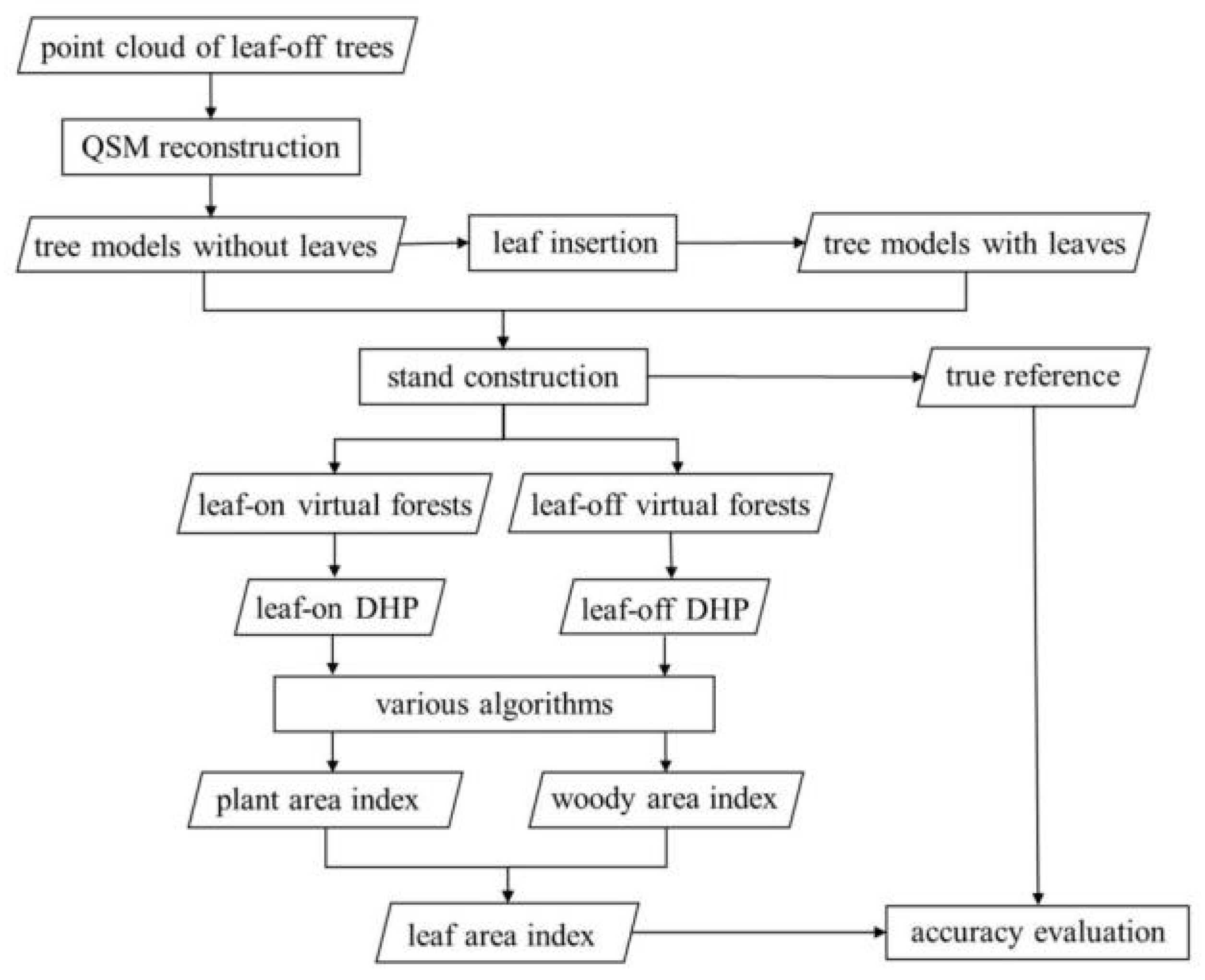
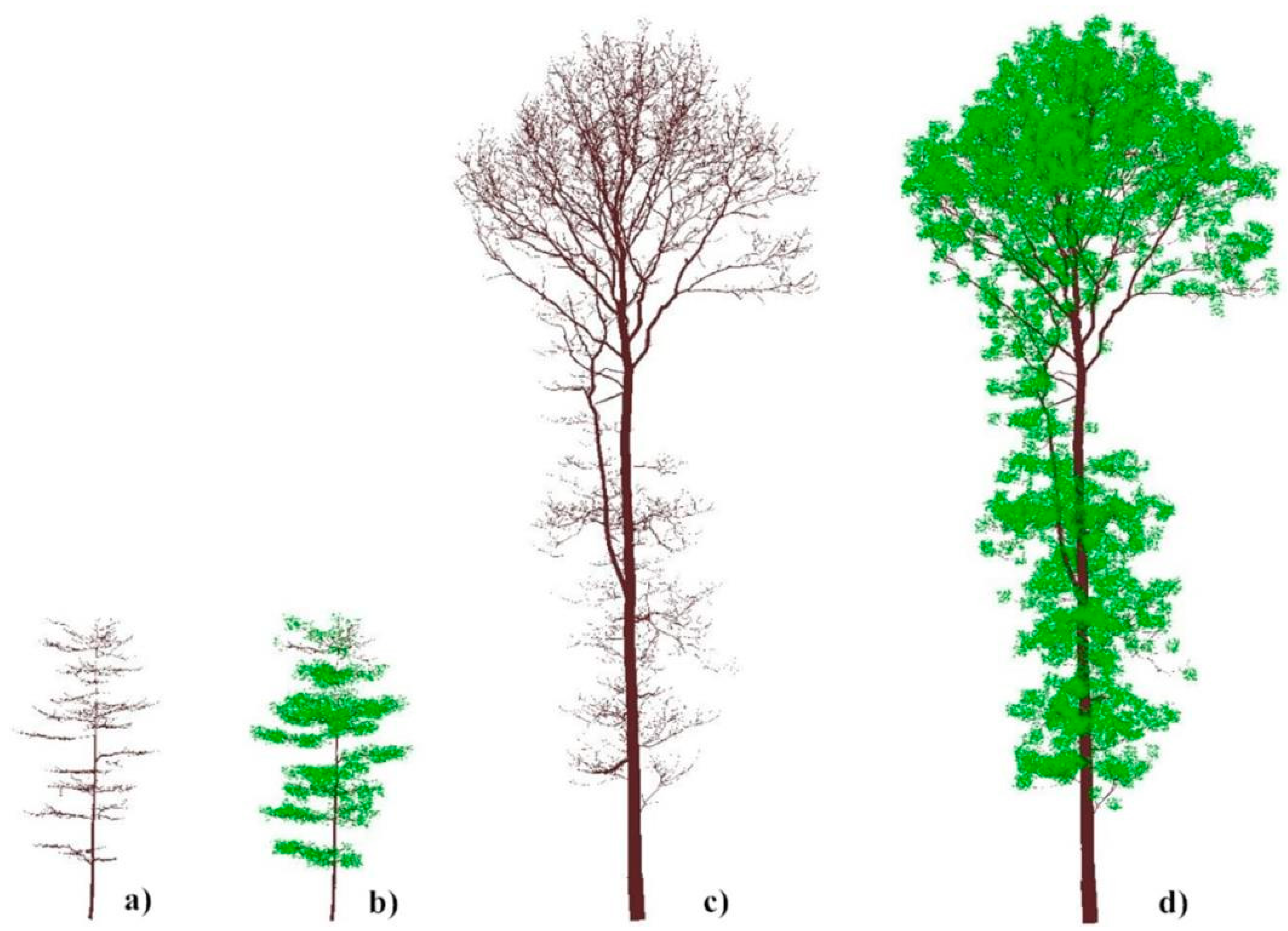
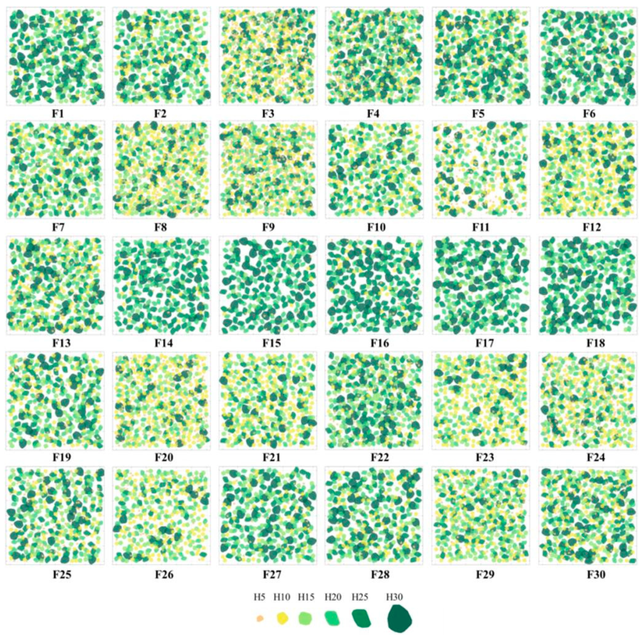
2.1. Virtual Forests Generation

Realistic tree models were used in this study to construct virtual broadleaf forests. Compared to the simple geometric primitives used in previous studies [43], realistic tree models are used to better simulate the complex structure of forest woody components. For each individual tree, the models for woody components and leaves were generated separately. The process began by reconstructing the 3D models of tree stems and branches with the open-source TreeQSM method as quantitative structure models (QSM) [52]. The TreeQSM method required point cloud data of single leaf-off trees as model inputs. In this study, we used the terrestrial laser scanning point cloud data of European beech (Fagus sylvatica) trees and English oak (Quercus robur L.) trees in leaf-off conditions, which were collected in previous studies [53,54]. A variety of individual trees was constructed, with the heights of 5, 10, 15, 20, 25, and 30 m. A diamond shape consisting of two triangles was used as the base leaf model for all trees. Various leaf sizes were utilized, ranging from 25 to 60 cm2. Leaves were inserted to the woody QSM model using a revised non-intersecting leaf insertion algorithm (QSM-FaNNI) [54], so that leaves intersected neither other leaves nor other woody components. Trees of different leaf densities were created. In addition, we revised the original QSM-FaNNI leaf insertion method so that the orientation of all leaves followed pre-defined leaf inclination angle distribution types. As a result, we received a collection of 180 highly realistic tree models, examples of which are shown in Figure 2.
Afterward, individual tree models were randomly distributed spatially to construct virtual forest stands. A total of 30 scenes were simulated comprising different LAI values and stem distributions as presented in Figure 3. Each forest stand had a size of 120 × 120 m. Each tree was placed with a random rotation around the vertical axis to increase randomness. Rules were defined so that the 3D convex hull of neighboring trees did not intersect with each other, with the implication that a small understory tree could stand beneath a tall tree. A flat topography was assumed for all stands in this study. The detailed stand information is illustrated in Table 1.
The ground-truthed LAI and PAI are termed LAItrue-ref and PAItrue-ref hereafter. They were derived directly from the virtual forest stands, by taking the ratio between “half of the total surface areas of all leaves and all woody components in the forest stand” and “the ground area of the forest stand”. To be consistent with the usual height of 1.5 m above ground for most DHP collections, only the leaves and woody components above this height were incorporated in the computation. The stand LAItrue-ref values ranged from 0.52 to 5.53, while the stand PAItrue-ref values ranged from 1.43 to 6.38. In each stand, a circular plot with a radius of 25 m was selected for taking DHP. The plot LAItrue-ref values ranged from 0.49 to 5.39, while the plot PAItrue-ref values ranged from 1.3 to 6.15. The LAItrue-ref and PAItrue-ref of each virtual forest stand are shown in Table 1.

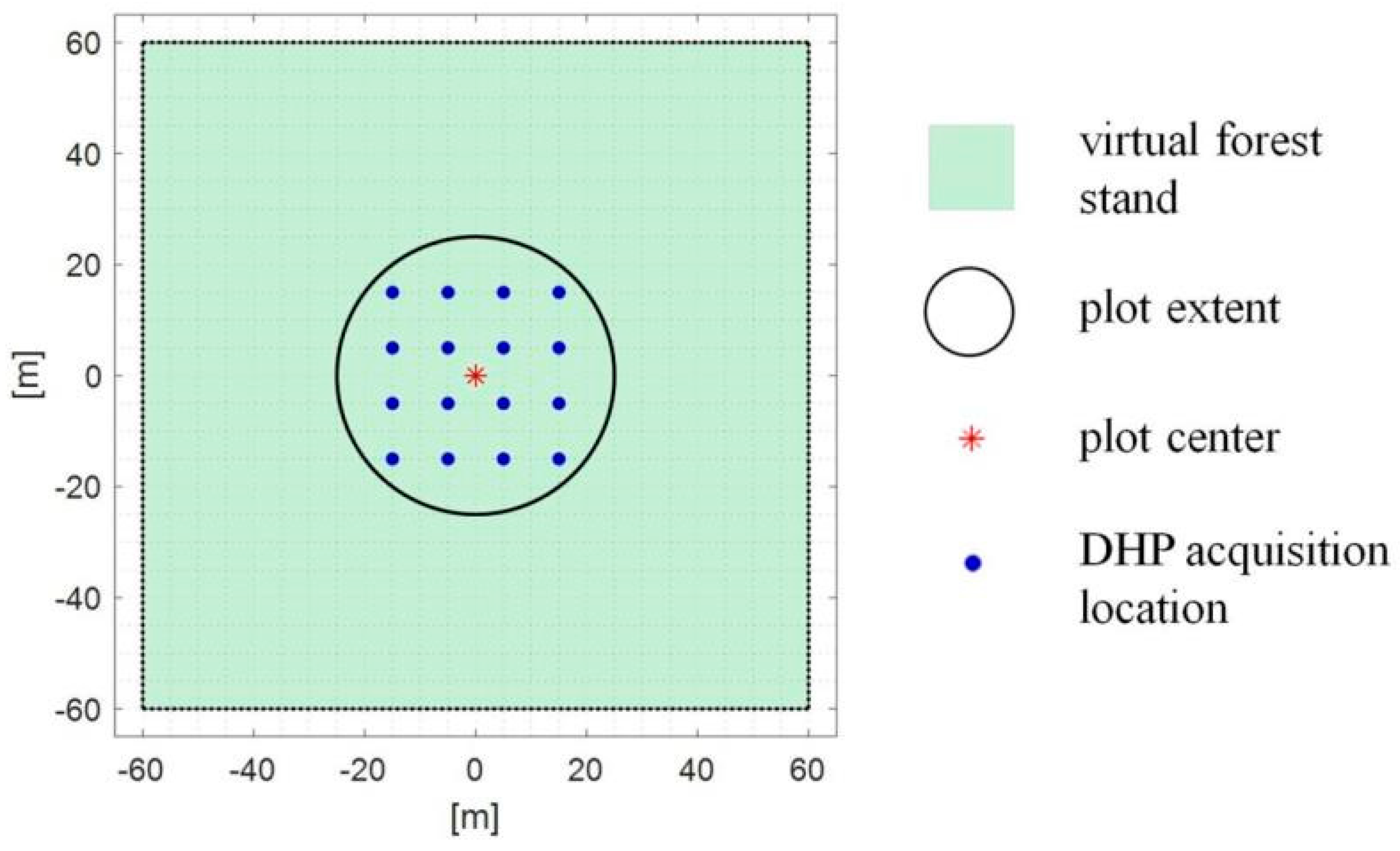
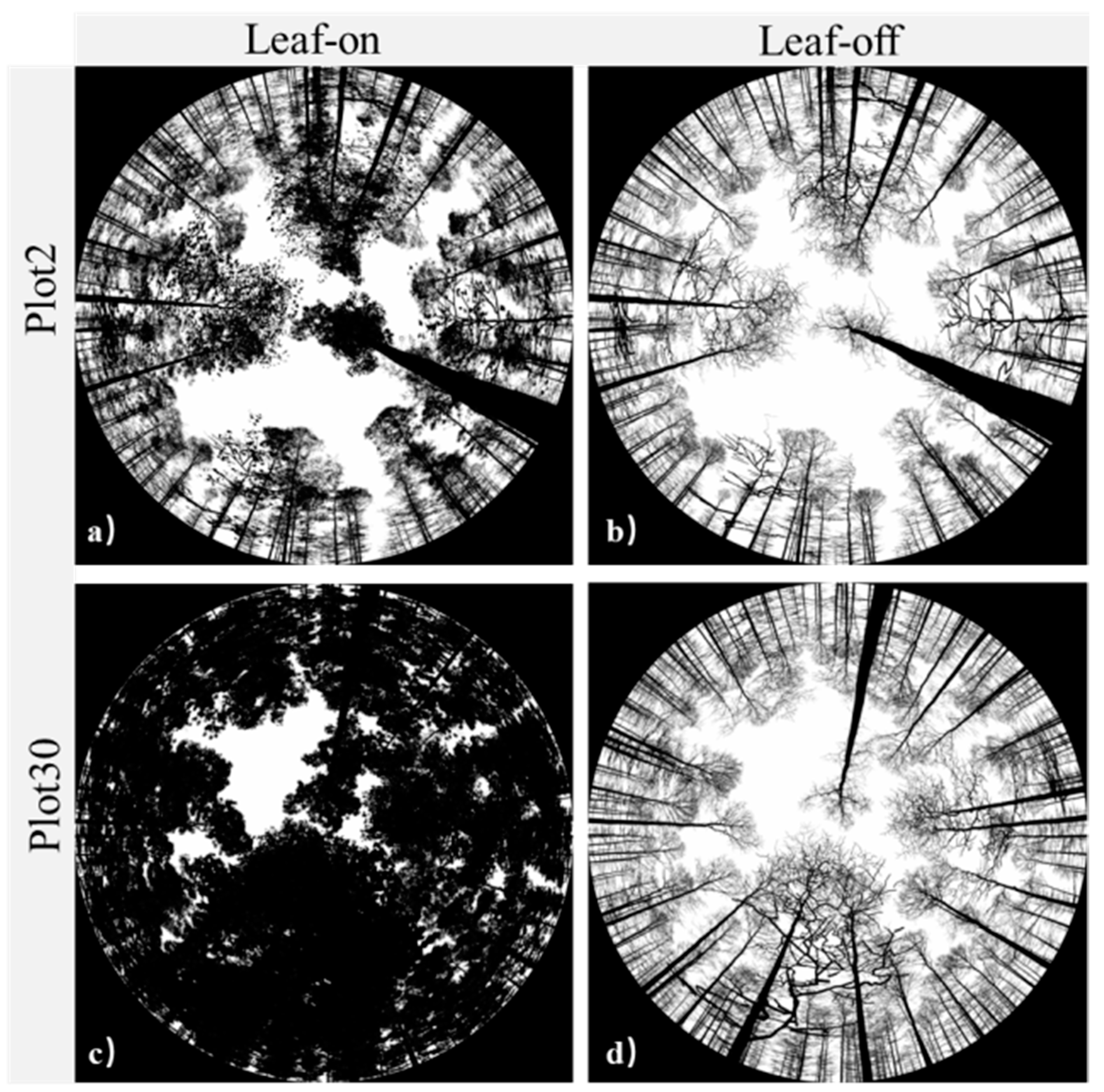
2.2. Synthetic DHP Generation

A ray-tracing tool, the POV-Ray software, was used to generate the synthetic DHP for the virtual forest stands. POV-Ray has been used in previous studies as well [43,45]. For each forest stand, the plot size had a 25 m radius. A regular grid sampling scheme was adopted as suggested by existing literature [17,55]. The specific DHP acquisition locations are displayed in Figure 4. In total, 16 DHP images were acquired for each plot, with the cameras placed 1.5 m above the ground. The image resolution of the synthetic DHP images was 3648 × 3648 pixels. The DHP images were generated for both leaf-on and leaf-off stands. Examples of the synthetic DHP images are presented in Figure 5.

2.3. LAI Estimation from DHP

Estimation of LAI from DHP generally relies on the gap fraction inversion. For canopies with randomly distributed leaves, the Poisson model can be used to relate the gap fraction at multiple directions with the amounts and orientations of leaves. For canopies with clumped leaves, models based on the negative binomial probability function were developed [56]. In forests, the effective PAI (PAIeff) and true PAI (PAItrue) can be related to gap fraction using the equations:
P ( θ ) = exp ( G ( θ ) PAI eff cos ( θ ) )
P ( θ ) =   exp ( G ( θ ) λ ( θ ) PAI true cos ( θ ) )
where θ is the zenith angle, P ( θ ) is the gap fraction in the θ direction, G( θ ) is the plant projection function value in the θ direction which is determined by the orientation of leaves and woody components [57]. The λ ( θ ) is the clumping index in the θ direction, which quantifies the degree to which canopy elements deviate from a random distribution. A λ value lower than 1 denotes a clumped distribution. The smaller λ is, the more clumped the canopy is. The determination of G( θ ) and λ ( θ ) are two challenges for PAI true estimation. Using the hinge angle at 57.5°, G( θ ) can be approximated as a constant value of 0.5 regardless of the orientation of plants [55]. It is also possible to use the Miller’s integral formula [58] without estimating G( θ ):
PAI eff = 2 0 π / 2 ln [ P ( θ ) ] cos ( θ ) sin ( θ ) d θ
However, it is biased if it is not possible to analyze the DHP in the 0°~90° range [55,59]. Another common method is to use a one-parameter or two-parameter function to model the leaf angle distribution g ( θ )   and the G( θ ), so as to inverse the G( θ ) and PAI from P ( θ ) observations at multiple directions [60,61,62].
To correct for canopy non-randomness and estimate PAItrue [55], three main methods were proposed to estimate the clumping index ( λ ( θ ) ), including the finite-length averaging method (LX) [63], the gap size distribution method (CC) [64,65], and the combination of LX and CC (CLX) method [66]. The finite-length averaging (LX) method was proposed by Lang and Xiang in 1986 using the following equation:
λ LX ( θ ) = ln P ( θ ) ¯ ln P ( θ ) ¯
where P ( θ ) ¯ is the canopy mean gap fraction of all segments, and ln P ( θ ) ¯ is the logarithmic mean from gap fractions of all segments [63]. However, two assumptions underlie this method, i.e., the foliage within the finite length segment is random, and the segment contains gaps. For segments completely obstructed by leaves, both Can_Eye and CIMES adopted a saturated LAI ( L sat ) value to address this problem. In this experiment, L sat was set as the default value of 10 following the manuals of Can_Eye and CIMES. The gap size distribution method was proposed by Chen and Cihlar in 1995 and corrected by Leblanc in 2002, using the following equation:
λ CC ( θ ) = ln [ F m ( 0 , θ ) ] [ 1 F m r ( 0 , θ ) ] ln [ F m r ( 0 , θ ) ] [ 1 F m ( 0 , θ ) ]
where F m ( 0 , θ ) is the accumulated canopy gap fraction, F m r ( 0 , θ ) is the reduced gap size accumulated fraction after removal of large non-random gaps from the measured gap size accumulation curve F m ( λ ) until the pattern of F m r ( 0 , θ ) resembles that of an equivalent canopy with a random spatial distribution of foliage [64,65]. In 2005, Leblanc proposed to combine the LX and the CC methods to address the potentially violated assumption of a random distribution of canopy elements at the segment scale associated with the LX method by using:
λ CLX ( θ ) = n ln [   P ( θ ) ¯   ] k = 1 n   ln [ P k ( θ ) ] / λ CCk ( θ )
where P k ( θ ) is the gap fraction of the segment k, and λ C C k ( θ ) is the clumping index of the segment k using the CC method. Another method to estimate PAI true consists of averaging values of local PAI eff over azimuthal angular intervals (WT method) [67].
Since forests contain many woody components other than leaves, a woody effect correction is necessary to convert the PAItrue to LAItrue. In this study, we used leaf-on and leaf-off DHP to estimate PAI and woody area index (WAI), respectively [68]. Then, the LAI was estimated using:
LAI true = PAI true WAI true
where PAItrue is the estimate of PAI after considering canopy non-randomness in leaf-on conditions, WAItrue is the estimate of WAI (PAI in leaf-off conditions) after considering canopy non-randomness, and LAItrue is the final estimate of LAI.
Specifically, all DHP images for both leaf-on and leaf-off virtual forests in this study were firstly processed with the automatic two-corner method to separate the sky from canopy pixels [69]. The two-corner method proved to be stable and more accurate than other methods based on previous studies [70]. After the image classification, the binary DHP images were imported into all DHP software, including Can_Eye, CIMES, and Hemisfer, for LAI estimation. In all software programs, the DHP was broken into multiple sub-sectors, with a 2.5° zenith angular resolution and a 10° azimuth angular resolution. The sub-sectors with zenith angles above 60° were removed from subsequent analysis due to a high portion of mixed pixels. All software are regularly improved and updated. The Can_Eye software was used is the version 6.495. The Hemisfer software was used is the version 3. For CIMES, we used the version (1982–2020).
In total, there were 37 algorithms from Can_Eye, CIMES, and Hemisfer producing PAItrue and LAItrue estimates (4 from Can_Eye, 9 from CIMES, and 24 from Hemisfer). The differences among these algorithms were mainly in how the PAIeff was estimated, how the orientation of leaves and the clumping index were estimated, and how pure canopy segments with zero gap fraction were handled. Summarized descriptions of the 37 algorithms are presented in Table 2, Table 3 and Table 4 for more details.
In general, Can_Eye offered estimates of PAIeff and PAItrue using either a single direction (57.5°) gap fraction or multidirectional (0°−60°) gap fraction with different inversion methods. The clumping index λ in Can_Eye was estimated based on the LX method [63]. Dissimilar to Can_Eye, CIMES was able to estimate λ not only using the LX but also using the CC and CLX methods [4]. The Hemisfer program implemented the LX and CC methods for clumping correction, as well as the non-linearity gap fraction correction. It is worth noting that even when using the same basic algorithm, the detailed procedures and inversion schemes may be inconsistent between different software. It is suggested to refer to the user manual of each software program for a more detailed description of each algorithm.

2.4. Statistical Analysis

In terms of the PAIeff and LAIeff, we calculated the consistency among the three programs (Can_Eye, CIMES, and Hemisfer), using the coefficient of determination (R2), and the root mean square difference (RMSD). Higher values of R2 and lower values of RMSD indicated greater consistency and robustness.
As for PAItrue and LAItrue, the values calculated from the virtual forests as described in Section 2.1 were used as the true reference values. Because the three programs offered 37 estimates of PAI and LAI from different algorithms, we first identified the most accurate results within each software program. In addition, the most accurate results were subsequently used for inter-software comparison, in terms of R2, RMSE, and normalized RMSE (nRMSE). Higher values of R2, lower values of RMSE, and lower values of nRMSE indicate higher accuracy.

3. Results

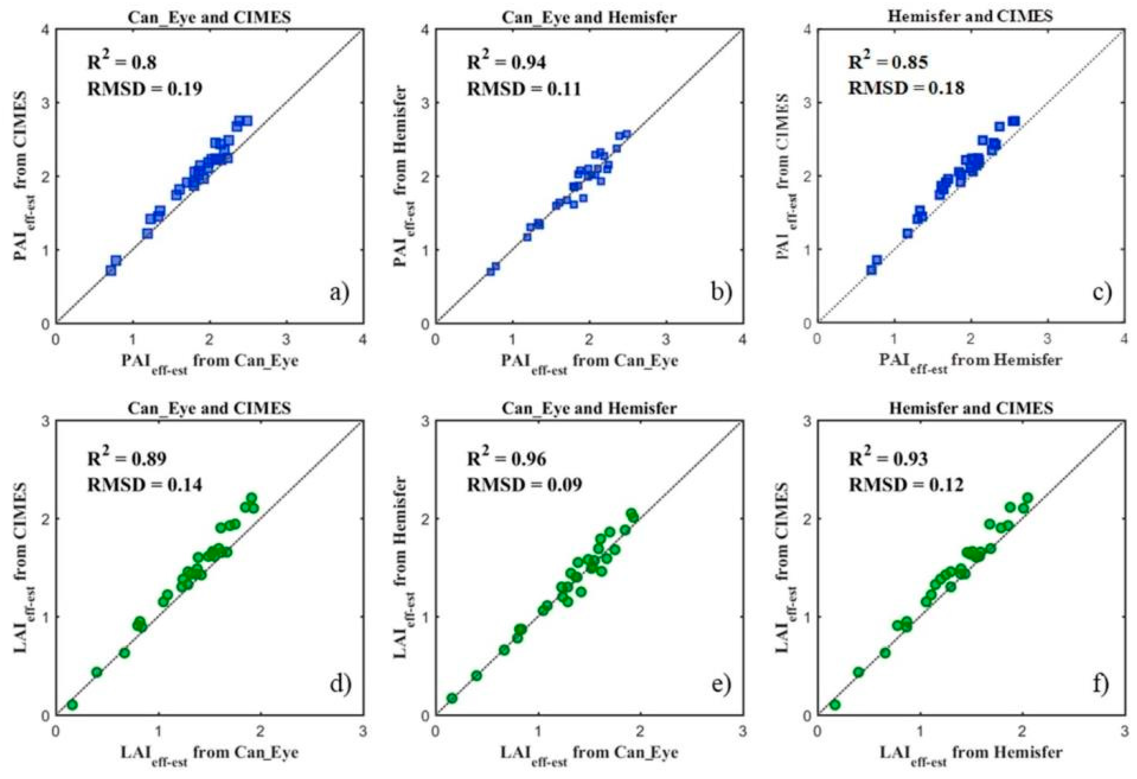
3.1. PAIeff and LAIeff Estimation Results

Without correcting for the clumping effect caused by vegetation non-randomness, the estimates of PAI (PAIeff-est) were on average 55.8% of the PAItrue-ref values, while the estimates of LAI (LAIeff-est) were on average 51.22% of LAItrue-ref values. The comparison of the PAIeff-est and LAIeff-est among the three programs is shown in Figure 6. The PAIeff and LAIeff estimates from CIMES were slightly higher than those from Can_Eye were (as shown in Figure 6a,d. Compared to CIMES, the PAIeff and LAIeff estimates from Hemisfer were closer to Can_Eye (RMSD = 0.11 < 0.19 for PAIeff-est, and RMSD = 0.09 < 0.14 for LAIeff-est, as shown in Figure 6b,e. In general, the results of effective PAI and effective LAI from the three programs were consistent (R2 ≥ 0.8, RMSD ≤ 0.19).

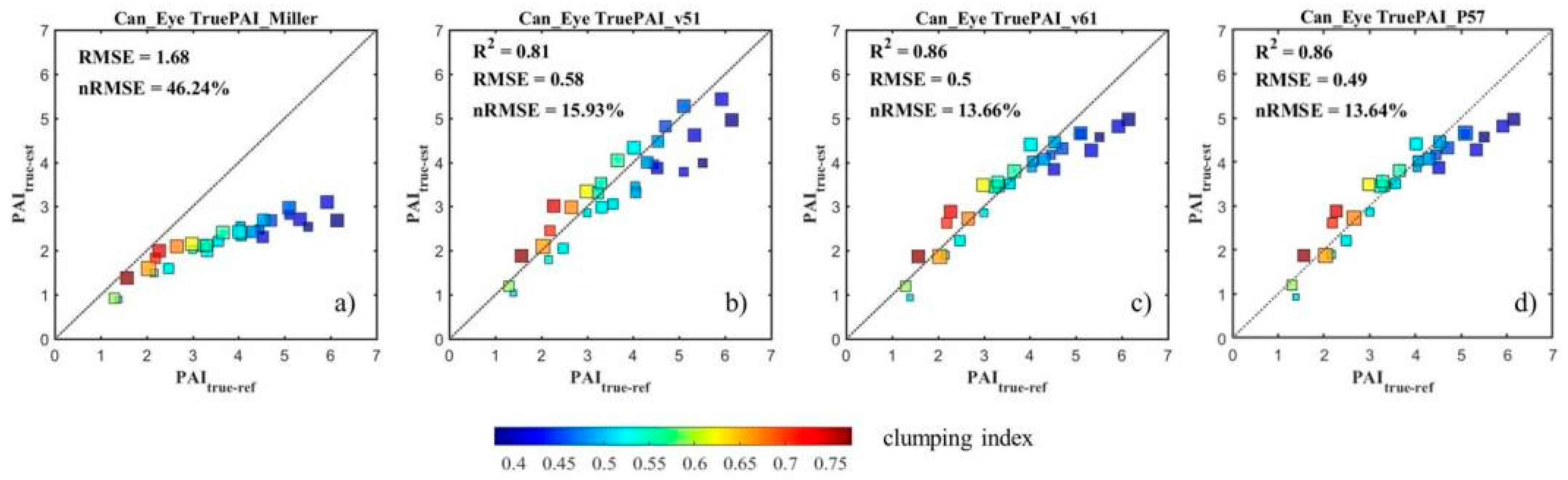
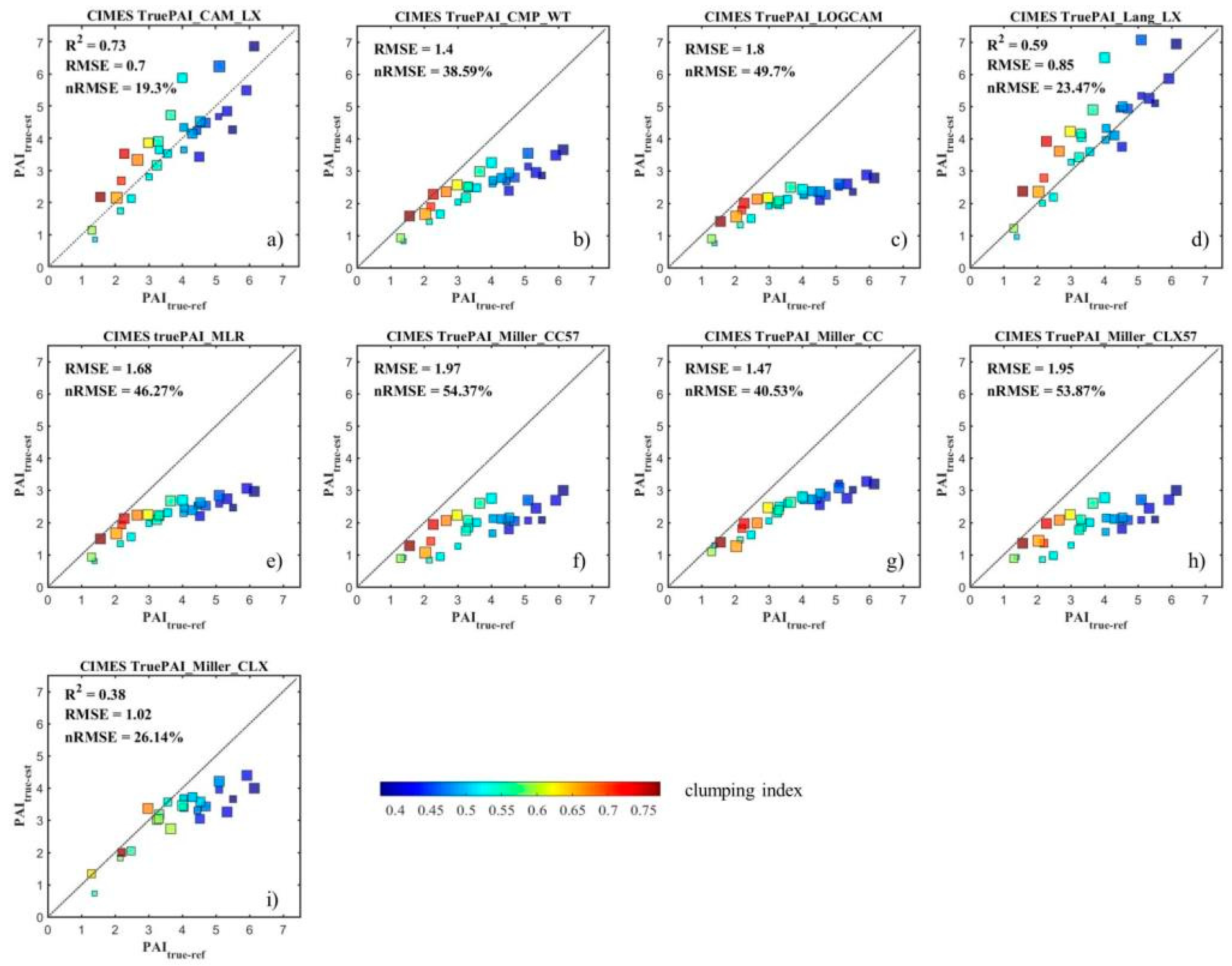
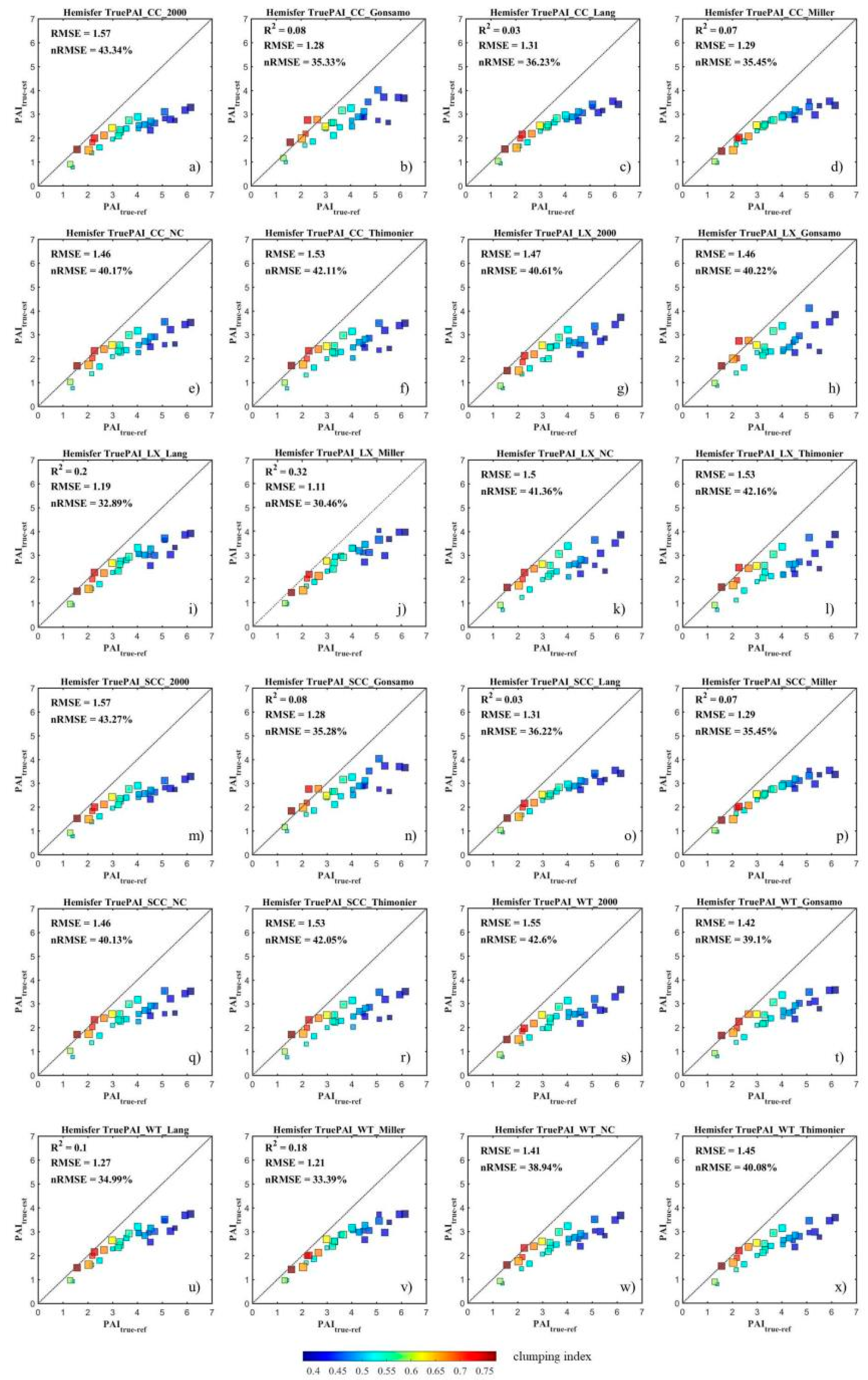
3.2. Comparison of PAItrue Estimation Accuracy

Using the PAIeff-est from Can_Eye divided by the plot PAItrue-ref, we obtained the clumping index values ( λ ) of each forest plot, as shown in Table 5. This quantified the level of the clumping effect in each stand and assisted in the evaluation of clumping correction methods using different algorithms.
All results of PAItrue-est using different algorithms in Can_Eye, CIMES, and Hemisfer are presented in Figure 7, Figure 8 and Figure 9, respectively. The symbol of each plot in each figure was colored based on the clumping index ( λ ) value according to the results in Table 5, and the size was adjusted according to the average leaf inclination angle of each plot in Table 1.
When comparing PAItrue-est with PAItrue-ref, the four algorithms in Can_Eye produced different PAItrue-est values, with nRMSE ranging in (13.64%, 46.24%) (see Figure 7). The most accurate algorithm was the P57 algorithm, which used the gap fraction (at 57.5°) inversion combined with the LX clumping correction method (R2 = 0.86, RMSE = 0.49, nRMSE = 13.64%). The least accurate algorithm in Can_Eye was Miller’s formula using the gap fraction at 0°~60° combined with the LX clumping correction method (RMSE = 1.68, nRMSE = 46.24%, see Figure 7).
In terms of CIMES, the nine algorithms produced quite different PAItrue-est values, with nRMSE ranging in (19.3%, 54.37%) (see Figure 8). The most accurate algorithm of CIMES was from the multiple direction gap fraction inversion at 0°~60° using the Campbell approach combined with the LX clumping correction (CAM_LX algorithm, R2 = 0.73, RMSE = 0.7, nRMSE = 19.3%), while the least accurate algorithm was the Miller_CC57 method, with the nRMSE reaching 54.37% (see Figure 8).
Regarding Hemisfer, the 24 algorithms produced different PAItrue-est values, with nRMSE ranging in (30.46%, 43.34%) (see Figure 9). The most accurate PAItrue-est result from Hemisfer was obtained with the LX_Miller method (R2 = 0.32, RMSE = 1.11, nRMSE = 30.46%), while the least accurate algorithm was the CC_2000 method, with the nRMSE reaching 43.34% (see Figure 9).
An inter-comparison among all 37 algorithms revealed that the most accurate algorithm to estimate PAItrue was the P57 method in Can_Eye, which used the gap fraction (at 57.5°) inversion combined with the LX clumping correction. Of note, there was a strong systematic underestimation of PAItrue by Hemisfer, either for canopies with high or low clumping. The PAItrue estimates from Hemisfer reached saturation at PAI values around three (Figure 9j). In comparison, the P57 method in Can_Eye could accurately correct the clumping effect until the vegetation reached high clumping (when λ < 0.45); then, it began to underestimate PAItrue in forests with PAI above 4.5 (Figure 7d). There was neither a systematic underestimation nor overestimation of PAItrue using the CAM_LX algorithm from CIMES (Figure 8a). In Figure 7d, Figure 8a and Figure 9j, there was no clear spatial distribution pattern of symbol sizes, implying that the average leaf inclination angle of each stand had little effect on the estimation of PAItrue.

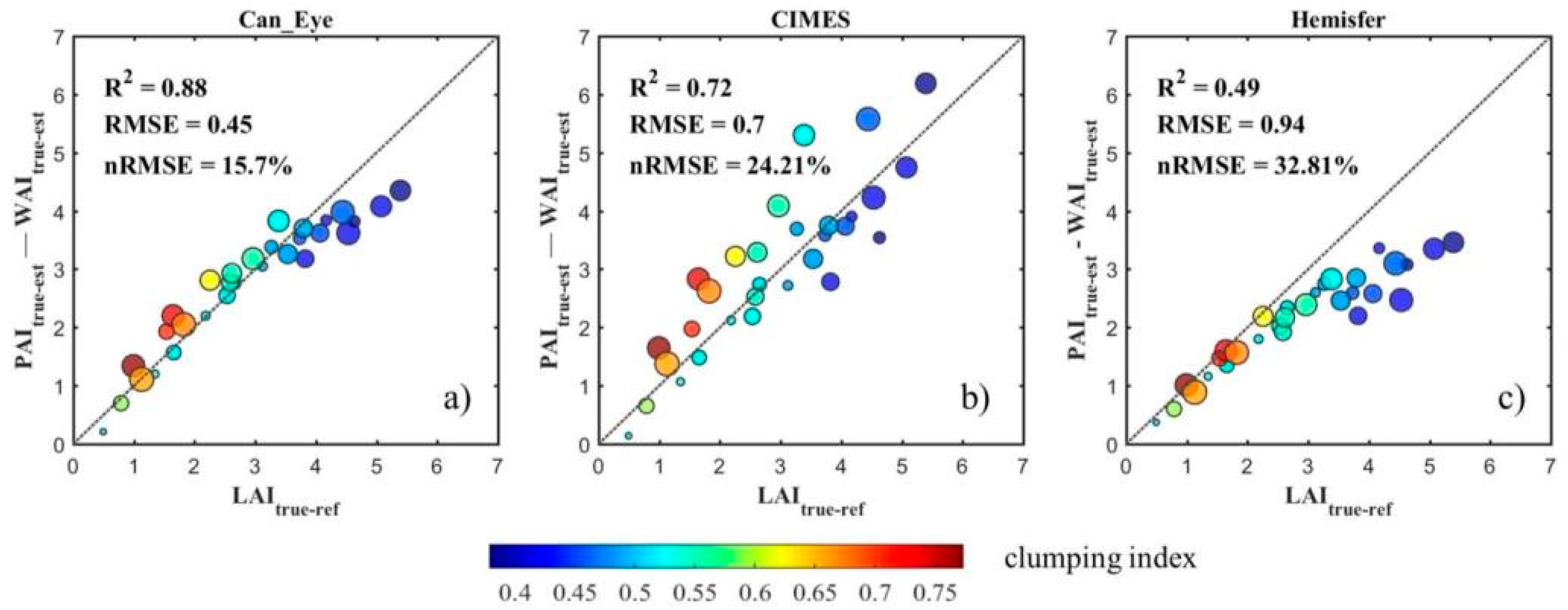
3.3. Comparison of LAItrue Estimation Accuracy

In terms of LAItrue-est, similar to the case of PAItrue-est, different algorithms produced quite different LAItrue-est results (nRMSE ranged in (15.7%, 53.24%) for Can_Eye, (24.21%, 70.64%) for CIMES, and (32.81%, 49.49%) for Hemisfer). Within each software program, the most accurate algorithm to estimate LAItrue was the same as PAItrue. For more details, the reader can refer to Figures S1–S3 in the Supplementary. In the following, only the most accurate algorithm in each software program was listed for an intercomparison.
The P57 method in Can_Eye which used the gap fraction (at 57.5°) inversion combined with the LX clumping correction was revealed as the most accurate algorithm to estimate LAItrue compared to CIMES and Hemisfer (R2 = 0.88 > 0.72, 0.49; RMSE = 0.45 < 0.7, 0.94; nRMSE = 15.7% < 24.21%, 32.81%, see Figure 10). There was a more severe underestimation of LAItrue from the LX_Miller algorithm in Hemisfer than from CIMES and Can_Eye, even in forests with a moderate amount of leaves at the LAI value around 2.5 (Figure 10c). In comparison, the P57 method in Can_Eye started to underestimate LAI in forests with dense leaves, with an LAI value around four (Figure 10a). There was neither a systematic underestimation nor overestimation of LAItrue from the CAM_LX algorithm in CIMES (Figure 10b).

4. Discussion

The results of this study demonstrated that three commonly used programs for DHP (including Can_Eye, CIMES, and Hemisfer) could estimate consistent effective PAI and effective LAI, though these programs were inconsistent when estimating true PAI and true LAI using the same DHP images (Figure 6, Figure 7, Figure 8, Figure 9 and Figure 10). Our results are in agreement with a previous study by Hall et al (2017), who also found similar PAIeff estimates, but significantly different estimates of PAItrue between Can_Eye and CIMES [37]. However, this previous study by Hall et al. only reported the inconsistency between Can_Eye and CIMES. The contribution of our research is that we proved that Can_Eye estimates more accurate PAItrue and LAItrue values than CIMES and Hemisfer. In addition, we identified the most accurate algorithm among all 37 algorithms as the P57 algorithm in Can_Eye. This can guide future users during the algorithm and software selection step when measuring in situ LAI from DHP. In addition, the use of virtual forests was not subject to inherent field measurement errors compared to litterfall collection or destructive sampling. It, thus, provides strong confidence in the results of the algorithm assessment.
The results of this study indicate that the major difference in estimating PAItrue and LAItrue among different software programs (i.e., Can_Eye, CIMES, and Hemisfer) was due to different estimates of the clumping index. Many researchers have pointed out that the estimates of the clumping index remained a large source of uncertainty for LAI estimation [44,75]. There was a systematic underestimation of PAItrue and LAItrue using Hemisfer, even in forests with a moderate amount of leaves and low vegetation clumping (as shown in Figure 9g–l and Figure S3g–l). This may have been caused by the pure canopy segments with no gaps. In such cases, the underlying assumption “the segment contains gaps” in the LX method did not hold. Both the Can_Eye and CIMES software utilized a saturated LAI ( L sat ) value to address this problem. In this experiment, L sat was set as 10 for both Can_Eye and CIMES. Dissimilar to Can_Eye and CIMES, Hemisfer did not provide this L sat solution and offered no details about how pure canopy segments were handled. This may be the reason for the systematic underestimation of PAItrue and LAItrue in Hemisfer.
The better performance of the P57 algorithm in Can_Eye was perhaps because it used the 57.5° angle when G( θ ) was approximated as 0.5, while other methods such as the v5.1 algorithm and the v6.1 algorithm in Can_Eye and the CAM_LX algorithm in CIMES used multiple directions (0°~60°) and had to inverse both the average leaf inclination angle (ALA) as well as PAI or LAI, which could add more uncertainty and errors (as shown in Figure 7b–c, Figure 8a, Figures S1b–c and S2a). Even using the same 0°~60° direction and the same LX clumping correction method, CIMES generated a less accurate PAItrue and less accurate LAItrue than Can_Eye (i.e., comparing Figure 8a with Figure 7b,c and comparing Figure S1a with Figure S2b,c in the Supplementary). This may be caused by the different inversion schemes implemented in Can_Eye and CIMES. Can_Eye introduces a regularization term in the cost function, which imposes constraints to improving the PAI estimates (see Equations (8) and (9)), while CIMES is not similarly constrained [4,19,59]. The higher accuracy of the v6.1 method than the v5.1 method in Can_Eye found in our study (R2 = 0.86 > 0.81, RMSE = 0.5 < 0.58, nRMSE = 13.66% < 15.93%, as shown in Figure 7) corroborates the prediction of higher efficiency of the PAI regularization term when compared with the ALA regularization term [19].
v 5.1   m e t h o d :   J k = i = 1 N b _ Z e n i t h _ D i r w i ( P L U T ( k ) ( θ i ) P M E S ( θ i ) ) 2 σ M O D ( P M E S ( θ i ) ) + ( A L A L U T ( k ) 60 30 ) 2
v 6.1   m e t h o d :   J k = i = 1 N b _ Z e n i t h _ D i r w i ( P L U T ( k ) ( θ i ) P M E S ( θ i ) ) 2 σ M O D ( P M E S ( θ i ) ) + ( P A I L U T ( k ) P A I 57 σ P A I 57 ) 2
In terms of the CC clumping correction method [64,65], there was a clear underestimation of PAItrue and LAItrue using CIMES and Hemisfer (as shown in Figure 8f,g, Figure 9a–f,m–r, Figures S2f,g and S3a–f,m–r in the Supplementary). This is in agreement with previous studies, which also found that the CC method underestimated the clumping effect (i.e., overestimation of λ [32,76].
Previous studies [32,43,66] suggested the CLX method worked better than the LX and CC method because it addressed the issues of “clumping within the segment”. Currently, only CIMES implemented the CLX clumping correction method. Therefore, this study cannot present a comparison among different software implementations of the CLX methods. However, in our study, we found that the CLX method using multiple directions (0°~60°) in CIMES generally failed to estimate the WAI using leaf-off DHP (see Figure S2i in the Supplementary). Further inspection revealed that the CLX estimate using the LAIMIL method in CIMES equaled 0. Currently, we cannot offer a clear explanation about this issue. It is suspected that there may have been some errors in the implementation of the CLX correction in the LAIMIL method. Nevertheless, it is suggested to be cautious using the CLX method in CIMES before its refinement and perhaps to incorporate the CLX method in Can_Eye, which may result in more accurate estimates of PAItrue and LAItrue.
The woody component was another obstacle for calculating the true LAI. One method to correct the woody effect was to multiply the estimate of PAI by a woody-to-total area ratio (α) to achieve WAI. An empirical α value could be estimated based on destructive sampling for a certain type of tree. Such manually intensive methods are dependent on species composition and growth form, and may not capture the spatial variation of α across stands [77]. The use of a near-infrared (NIR) channel camera to differentiate between woody and foliar components has been suggested but has not been applied widely [78]. Some studies combined the use of DHP acquired in leaf-on and leaf-off conditions for broadleaf forests, to estimate LAI by subtracting leaf-off PAI from leaf-on PAI [68], though the results were not validated. The study by Calders et al. (2018) proved that subtraction of WAIeff from PAIeff correlated well with LAIeff when using a virtual forest [79]. The results of our study further illustrated that the subtraction of WAItrue from PAItrue correlated well with pre-defined LAItrue values (Figure 10). This demonstrated the effectiveness of using leaf-on and leaf-off DHP to correct the woody effect and estimate LAI for broadleaf forests. This can also provide a reference for dynamic LAItrue monitoring studies using repeated DHP for broader environmental applications [80].
Continuous and freely available satellite LAI products have boosted global Earth system modeling studies [15]. However, an inconsistency was found in different satellite LAI products such as GLASS, LAI3g, TCDR, and GLOBMAP [81]. Many more in situ LAI measurements are in great need to enhance the accuracy of satellite LAI products [1]. Previous studies have highlighted the uncertainty in in situ LAI measurements using different techniques, including DHP, terrestrial LiDAR, and LAI-2200 [70]. Our study highlighted the inconsistency of LAI estimates from DHP using different algorithms from various software programs. It proves that care must be taken, and analysts should carefully follow a methodological protocol while processing the DHP for LAI estimates. The finding of this study can guide the expansion of ground LAI observation networks, which is vital to enhance the quality of satellite products [16]. Further studies must be implemented to consolidate the accuracy of in situ LAI measurements, which is the basis for calibrating and validating satellite LAI products for downstream applications.
Virtual forests can play an important role in refining in situ LAI estimation methods, since high-fidelity, ground-reference LAI, such as that from destructive measurements, is rarely available at stand level. To acquire true values of LAI and PAI in real forests, we would need to destructively sample all leaves and woody components and measure their surface area in forests. This is too expensive and impractical. Although the litterfall collection method can be used to estimate true LAI, it is prone to uncertainty caused by litter trap frequency and collection time intervals [82]. However, in the set-up of virtual forests, we can control and calculate all aspects ranging from each leaf to each branch of the forests. The virtual forest created in this research had PAI values ranging from 1.43 to 6.38, which is consistent with a previous study that shows a range of PAI values from 1.1 to 8.0 in temperate deciduous broadleaf forests [83]. In addition, the clumping index ranging from 0.38 to 0.78 in this study is also similar to the range of 0.41 to 0.92 for clumping indices of forests derived from MODIS data in previous studies [84,85]. This strengthens the reliability of the virtual forest generation framework employed in this research. Further studies may adopt the actual position of individual trees from the forest inventory instead of random displacements of trees. A recent approach named “Canopy Constructor”, which combines field inventories and airborne LiDAR scans to create virtual forests that best fit the data, is a promising method [86]. Virtual forests can be used in the algorithm development stage as well as indoor evaluation at low cost. It offers the possibility for DHP re-collection, which is useful when a new LAI collection protocol is designed. Although field measurement is still indispensable, virtual forests can serve as a supplement for validating the theoretical error of each factor inherent in LAI measurement and retrieval [87].
Several limitations can be addressed in future relevant research. Firstly, the current study assumed a relatively small forest size due to the limitation of computing resources. Secondly, for simplicity, our study assumed a flat terrain and pure broadleaf stands in all virtual forests. Given that much progress has been achieved in reconstructing highly realistic coniferous trees from terrestrial LiDAR point clouds [88,89], future studies can investigate the accuracy of in situ LAI measurement in virtual coniferous or mixed forests and mountainous forests.

5. Conclusions

DHP is a widely used in situ LAI technique, which was used to collect LAI ground references for improving satellite LAI products. Given the array of various algorithms and software programs that are available for processing DHP for LAI estimation, an accuracy evaluation among these methods has become urgent. There have been few studies comparing the accuracy of these algorithms in forests due to the difficulty in achieving a high-fidelity reference LAI value. This study used virtual forests to address this issue. Various broadleaf forests covering a range of tree heights, stem densities, and LAI values were constructed. Combined with ray-tracing, a synthetic DHP was simulated, both for leaf-on and leaf-off conditions. A total of 37 algorithms from three programs, including Can_Eye, CIMES, and Hemisfer, were used to estimate the plant area index (PAI) from leaf-on DHP, woody area index (WAI) from leaf-off DHP, and LAI by subtracting WAI from PAI. Other software such as the Gap Light Analyzer and HemiView were not investigated in this study since they do not correct for the clumping effect. Overall, the results demonstrated that effective PAI and LAI results could be consistently retrieved from the three programs (R2 > 0.8, RMSD < 0.2). However, after correcting for the clumping effect caused by a non-random vegetation distribution, a large inconsistency occurred between the estimates of true PAI and true LAI from different algorithms. The results demonstrated that Can_Eye more accurately estimated true LAI than CIMES and Hemisfer (with R2 = 0.88 > 0.72, 0.49; RMSE = 0.45 < 0.7, 0.94; nRMSE = 15.7% < 24.21%, 32.81%). It was also found that the P57 algorithm, which used the 57.5° gap fraction inversion combined with the finite-length averaging (LX) clumping correction method implemented in Can_Eye, was the most accurate. This study highlighted the in situ LAI measurement uncertainty due to the choice of the LAI algorithm and demonstrated the effectiveness of using leaf-on and leaf-off to correct for the woody component’s effect on LAI estimation. From the results of this study, we recommend using the 57.5° gap fraction inversion combined with the finite-length averaging (LX) clumping correction method implemented in Can_Eye for LAI estimation in broadleaf forests. Further studies exploring coniferous and mixed forests are suggested to consolidate the protocol of in situ LAI measurements to reduce in situ LAI uncertainty.

Supplementary Materials

The following supplementary materials are in the Supplementary available online at https://0-www-mdpi-com.brum.beds.ac.uk/article/10.3390/rs13163325/s1, Figure S1: LAI true results using different algorithms from Can_Eye, Figure S2: LAI true results using different algorithms from CIMES, Figure S3:  LAI true results using different algorithms from Hemisfer.

Author Contributions

Conceptualization, J.L, L.L. and T.W.; methodology, J.L., T.W. and A.S.; analysis and validation, J.L; resources and data curation, M.A., X.Z. and M.H.; writing—original draft preparation, J.L.; writing—review and editing, all authors. All authors have read and agreed to the published version of the manuscript.

Funding

This research was funded by the National Key Research and Development Program of China (2017YFA0603603), the National Natural Science Foundation of China (No: 42001284), the Jiangsu Natural Science Foundation (No: BK20200722), the Natural Science Foundation of the Jiangsu Higher Education Institutions of China (No: 20KJB420001), and the Horizon 2020 research and innovation programme—European Commission ’BIOSPACE Monitoring Biodiversity from Space’ project (grant agreement ID 834709, H2020-EU.1.1).

Data Availability Statement

The data presented in this study are available on request from the corresponding author.

Acknowledgments

The authors acknowledge the anonymous reviewers and the editor for giving advice on improving the quality of this work. The authors acknowledge the support of the “Remote Sensing Data Pool Initiative for the Bohemian Forest Ecosystem” data-sharing initiative of the Bavarian Forest National Park.

Conflicts of Interest

The authors declare no conflict of interest.

References

  1. Fernandes, R.; Plummer, S.; Nightingale, J.; Baret, F.; Camacho, F.; Fang, H.; Garrigues, S.; Gobron, N.; Lang, M.; Lacaze, R.; et al. Global Leaf Area Index Product Validation Good Practices. Version 2.0. 2014; p. 76. Available online: https://lpvs.gsfc.nasa.gov/LAI/LAI_home.html (accessed on 15 June 2021).
  2. Skidmore, A.K.; Pettorelli, N. Agree on biodiversity metrics to track from space: Ecologists and space agencies must forge a global monitoring strategy. Nature 2015, 523, 403–406. [Google Scholar] [CrossRef] [Green Version]
  3. Bojinski, S.; Verstraete, M.; Peterson, T.C.; Richter, C.; Simmons, A.; Zemp, M. The concept of essential climate variables in support of climate research, applications, and policy. Bull. Am. Meteorol. Soc. 2014, 95, 1431–1443. [Google Scholar] [CrossRef]
  4. Gonsamo, A.; Walter, J.-M.N.; Pellikka, P. CIMES: A package of programs for determining canopy geometry and solar radiation regimes through hemispherical photographs. Comput. Electron. Agric. 2011, 79, 207–215. [Google Scholar] [CrossRef]
  5. White, K.; Pontius, J.; Schaberg, P. Remote sensing of spring phenology in northeastern forests: A comparison of methods, field metrics and sources of uncertainty. Remote Sens. Environ. 2014, 148, 97–107. [Google Scholar] [CrossRef]
  6. Lang, M.; Nilson, T.; Kuusk, A.; Pisek, J.; Korhonen, L.; Uri, V. Digital photography for tracking the phenology of an evergreen conifer stand. Agric. For. Meteorol. 2017, 246, 15–21. [Google Scholar] [CrossRef]
  7. Baret, F.; Weiss, M.; Allard, D.; Garrigue, S.; Leroy, M.; Jeanjean, H.; Fernandes, R.; Myneni, R.; Privette, J.; Morisette, J.; et al. VALERI: A network of sites and a methodology for the validation of medium spatial resolution land satellite products. Remote Sens. Environ. 2005, 76, 36–39. [Google Scholar]
  8. Brown, L.A.; Meier, C.; Morris, H.; Pastor-Guzman, J.; Bai, G.; Lerebourg, C.; Gobron, N.; Lanconelli, C.; Clerici, M.; Dash, J. Evaluation of global leaf area index and fraction of absorbed photosynthetically active radiation products over North America using Copernicus Ground Based Observations for Validation data. Remote Sens. Environ. 2020, 247, 111935. [Google Scholar] [CrossRef]
  9. Li, X.J.; Mao, F.J.; Du, H.Q.; Zhou, G.M.; Xu, X.J.; Han, N.; Sun, S.B.; Gao, G.L.; Chen, L. Assimilating leaf area index of three typical types of subtropical forest in China from MODIS time series data based on the integrated ensemble Kalman filter and PROSAIL model. ISPRS J. Photogramm. Remote Sens. 2017, 126, 68–78. [Google Scholar] [CrossRef]
  10. Dong, T.F.; Liu, J.G.; Qian, B.D.; He, L.M.; Liu, J.; Wang, R.; Jing, Q.; Champagne, C.; McNairn, H.; Powers, J.; et al. Estimating crop biomass using leaf area index derived from Landsat 8 and Sentinel-2 data. ISPRS J. Photogramm. Remote Sens. 2020, 168, 236–250. [Google Scholar] [CrossRef]
  11. Zhu, X.; Liu, J.; Skidmore, A.K.; Premier, J.; Heurich, M. A voxel matching method for effective leaf area index estimation in temperate deciduous forests from leaf-on and leaf-off airborne LiDAR data. Remote Sens. Environ. 2020, 240, 111696. [Google Scholar] [CrossRef]
  12. Korhonen, L.; Korpela, I.; Heiskanen, J.; Maltamo, M. Airborne discrete-return LIDAR data in the estimation of vertical canopy cover, angular canopy closure and leaf area index. Remote Sens. Environ. 2011, 115, 1065–1080. [Google Scholar] [CrossRef]
  13. Liu, J.; Skidmore, A.K.; Jones, S.; Wang, T.; Heurich, M.; Zhu, X.; Shi, Y. Large off-nadir scan angle of airborne LiDAR can severely affect the estimates of forest structure metrics. ISPRS J. Photogramm. Remote Sens. 2018, 136, 13–25. [Google Scholar] [CrossRef]
  14. Tang, H.; Brolly, M.; Zhao, F.; Strahler, A.H.; Schaaf, C.L.; Ganguly, S.; Zhang, G.; Dubayah, R. Deriving and validating Leaf Area Index (LAI) at multiple spatial scales through lidar remote sensing: A case study in Sierra National Forest, CA. Remote Sens. Environ. 2014, 143, 131–141. [Google Scholar] [CrossRef]
  15. Fang, H.; Baret, F.; Plummer, S.; Schaepman-Strub, G. An overview of global leaf area index (LAI): Methods, products, validation, and applications. Rev. Geophys. 2019, 57, 739–799. [Google Scholar] [CrossRef]
  16. Piao, S.; Wang, X.; Park, T.; Chen, C.; Lian, X.; He, Y.; Bjerke, J.W.; Chen, A.; Ciais, P.; Tømmervik, H.; et al. Characteristics, drivers and feedbacks of global greening. Nat. Rev. Earth Environ. 2020, 1, 14–27. [Google Scholar] [CrossRef]
  17. Chianucci, F.; Cutini, A. Digital hemispherical photography for estimating forest canopy properties: Current controversies and opportunities. IForest-Biogeosci. For. 2012, 5, 290. [Google Scholar] [CrossRef] [Green Version]
  18. Frazer, G. Gap Light Analyzer (GLA) Imaging Software to Extract Canopy Structure and Gap Light Transmission Indices from True-Colour Fisheye Photographs, Users Manual and Program Documentation; Millbrook: New York, NY, USA, 1999; p. 36. [Google Scholar]
  19. Weiss, M.; Baret, F. CAN_EYE V6. 4.91 User Manual. Recuperado 2017, 12, 56. [Google Scholar]
  20. Schleppi, P.; Conedera, M.; Sedivy, I.; Thimonier, A. Correcting non-linearity and slope effects in the estimation of the leaf area index of forests from hemispherical photographs. Agric. For. Meteorol. 2007, 144, 236–242. [Google Scholar] [CrossRef]
  21. Morsdorf, F.; Kötz, B.; Meier, E.; Itten, K.; Allgöwer, B. Estimation of LAI and fractional cover from small footprint airborne laser scanning data based on gap fraction. Remote Sens. Environ. 2006, 104, 50–61. [Google Scholar] [CrossRef]
  22. Hymus, G.J.; Pontailler, J.Y.; Li, J.; Stiling, P.; Hinkle, C.R.; Drake, B.G. Seasonal variability in the effect of elevated CO2 on ecosystem leaf area index in a scrub-oak ecosystem. Glob. Chang. Biol. 2002, 8, 931–940. [Google Scholar] [CrossRef]
  23. Rudic, T.E.; McCulloch, L.A.; Cushman, K.C. Comparison of Smartphone and Drone Lidar Methods for Characterizing Spatial Variation in PAI in a Tropical Forest. Remote Sens. 2020, 12, 1765. [Google Scholar] [CrossRef]
  24. Canisius, F.; Fernandes, R.; Chen, J. Comparison and evaluation of Medium Resolution Imaging Spectrometer leaf area index products across a range of land use. Remote Sens. Environ. 2010, 114, 950–960. [Google Scholar] [CrossRef]
  25. De Kauwe, M.G.; Disney, M.I.; Quaife, T.; Lewis, P.; Williams, M. An assessment of the MODIS collection 5 leaf area index product for a region of mixed coniferous forest. Remote Sens. Environ. 2011, 115, 767–780. [Google Scholar] [CrossRef]
  26. Rowland, L.; da Costa, A.C.L.; Galbraith, D.R.; Oliveira, R.S.; Binks, O.J.; Oliveira, A.A.R.; Pullen, A.M.; Doughty, C.E.; Metcalfe, D.B.; Vasconcelos, S.S.; et al. Death from drought in tropical forests is triggered by hydraulics not carbon starvation. Nature 2015, 528, 119–122. [Google Scholar] [CrossRef] [Green Version]
  27. Demarez, V.; Duthoit, S.; Baret, F.; Weiss, M.; Dedieu, G. Estimation of leaf area and clumping indexes of crops with hemispherical photographs. Agric. For. Meteorol. 2008, 148, 644–655. [Google Scholar] [CrossRef] [Green Version]
  28. Zhu, X.; Skidmore, A.K.; Darvishzadeh, R.; Niemann, K.O.; Liu, J.; Shi, Y.; Wang, T. Foliar and woody materials discriminated using terrestrial LiDAR in a mixed natural forest. Int. J. Appl. Earth Obs. Geoinf. 2018, 64, 43–50. [Google Scholar] [CrossRef]
  29. Moeser, D.; Stahli, M.; Jonas, T. Improved snow interception modeling using canopy parameters derived from airborne LiDAR data. Water Resour. Res. 2015, 51, 5041–5059. [Google Scholar] [CrossRef] [Green Version]
  30. Thimonier, A.; Sedivy, I.; Schleppi, P. Estimating leaf area index in different types of mature forest stands in Switzerland: A comparison of methods. Eur. J. For. Res. 2010, 129, 543–562. [Google Scholar] [CrossRef]
  31. Ali, A.M.; Skidmore, A.K.; Darvishzadeh, R.; van Duren, I.; Holzwarth, S.; Mueller, J. Retrieval of forest leaf functional traits from HySpex imagery using radiative transfer models and continuous wavelet analysis. ISPRS J. Photogramm. Remote Sens. 2016, 122, 68–80. [Google Scholar] [CrossRef] [Green Version]
  32. Pisek, J.; Lang, M.; Nilson, T.; Korhonen, L.; Karu, H. Comparison of methods for measuring gap size distribution and canopy nonrandomness at Järvselja RAMI (RAdiation transfer Model Intercomparison) test sites. Agric. For. Meteorol. 2011, 151, 365–377. [Google Scholar] [CrossRef]
  33. Gonsamo, A.; Pellikka, P. Methodology comparison for slope correction in canopy leaf area index estimation using hemispherical photography. For. Ecol. Manag. 2008, 256, 749–759. [Google Scholar] [CrossRef]
  34. Glatthorn, J.; Beckschäfer, P. Standardizing the Protocol for Hemispherical Photographs: Accuracy Assessment of Binarization Algorithms. PLoS ONE 2014, 9, e111924. [Google Scholar] [CrossRef] [PubMed] [Green Version]
  35. Jarčuška, B.; Kucbel, S.; Jaloviar, P. Comparison of output results from two programmes for hemispherical image analysis: Gap Light Analyser and WinScanopy. J. For. Sci. 2010, 56, 147–153. [Google Scholar] [CrossRef] [Green Version]
  36. Promis, A.; Gärtner, S.; Butler-Manning, D.; Durán-Rangel, C.; Reif, A.; Cruz, G.; Hernandez, L. Comparison of four different programs for the analysis of hemispherical photographs using parameters of canopy structure and solar radiation transmittance. Sierra 2011, 519, 36. [Google Scholar]
  37. Hall, R.J.; Côté, J.-F.; Mailly, D.; Fournier, R.A. Comparison of software tools for analysis of hemispherical photographs. In Hemispherical Photography in Forest Science: Theory, Methods, Applications; Springer: Berlin/Heidelberg, Germany, 2017; pp. 187–226. [Google Scholar]
  38. Liu, Z.L.; Jin, G.Z.; Chen, J.M.; Qi, Y.J. Evaluating optical measurements of leaf area index against litter collection in a mixed broadleaved-Korean pine forest in China. Trees-Struct. Funct. 2015, 29, 59–73. [Google Scholar] [CrossRef]
  39. Fang, H.L.; Ye, Y.C.; Liu, W.W.; Wei, S.S.; Ma, L. Continuous estimation of canopy leaf area index (LAI) and clumping index over broadleaf crop fields: An investigation of the PASTIS-57 instrument and smartphone applications. Agric. For. Meteorol. 2018, 253, 48–61. [Google Scholar] [CrossRef]
  40. Hyyppa, J. Virtual Forest. 2019. Available online: https://0-www-mdpi-com.brum.beds.ac.uk/journal/remotesensing/special_issues/Virtual_Forest (accessed on 15 June 2021).
  41. Calders, K.; Origo, N.; Burt, A.; Disney, M.; Nightingale, J.; Raumonen, P.; Akerblom, M.; Malhi, Y.; Lewis, P. Realistic Forest Stand Reconstruction from Terrestrial LiDAR for Radiative Transfer Modelling. Remote Sens. 2018, 10, 933. [Google Scholar] [CrossRef] [Green Version]
  42. Uusitalo, J.; Orland, B. Virtual Forest Management: Possibilities and Challenges. Int. J. For. Eng. 2001, 12, 57–66. [Google Scholar] [CrossRef]
  43. Leblanc, S.; Fournier, R. Hemispherical photography simulations with an architectural model to assess retrieval of leaf area index. Agric. Forest Meteorol. 2014, 194, 64–76. [Google Scholar] [CrossRef]
  44. Gonsamo, A.; Pellikka, P. The computation of foliage clumping index using hemispherical photography. Agric. For. Meteorol. 2009, 149, 1781–1787. [Google Scholar] [CrossRef]
  45. Liu, J.; Wang, T.; Skidmore, A.K.; Jones, S.; Heurich, M.; Beudert, B.; Premier, J. Comparison of terrestrial LiDAR and digital hemispherical photography for estimating leaf angle distribution in European broadleaf beech forests. ISPRS J. Photogramm. Remote Sens. 2019, 158, 76–89. [Google Scholar] [CrossRef]
  46. Cao, B.; Du, Y.M.; Li, J.; Li, H.; Li, L.; Zhang, Y.; Zou, J.; Liu, Q.H. Comparison of Five Slope Correction Methods for Leaf Area Index Estimation From Hemispherical Photography. IEEE Geosci. Remote. Sens. Lett. 2015, 12, 1958–1962. [Google Scholar] [CrossRef]
  47. Raumonen, P.; Casella, E.; Calders, K.; Murphy, S.; Åkerbloma, M.; Kaasalainen, M. Massive-scale tree modelling from TLS data. In Proceedings of the Pia15+hrigi15—Joint Isprs Conference, Munich, Germany, 5–27 March 2015; pp. 189–196. [Google Scholar]
  48. Woodgate, W.; Armston, J.D.; Disney, M.; Suarez, L.; Jones, S.D.; Hill, M.J.; Wilkes, P.; Soto-Berelov, M. Validating canopy clumping retrieval methods using hemispherical photography in a simulated Eucalypt forest. Agric. For. Meteorol. 2017, 247, 181–193. [Google Scholar] [CrossRef]
  49. Zou, J.; Zhuang, Y.; Chianucci, F.; Mai, C.; Lin, W.; Leng, P.; Luo, S.; Yan, B. Comparison of Seven Inversion Models for Estimating Plant and Woody Area Indices of Leaf-on and Leaf-off Forest Canopy Using Explicit 3D Forest Scenes. Remote Sens. 2018, 10, 1297. [Google Scholar] [CrossRef] [Green Version]
  50. Wei, S.S.; Yin, T.G.; Dissegna, M.A.; Whittle, A.J.; Ow, G.L.F.; Yusof, M.L.M.; Lauret, N.; Gastellu-Etchegorry, J.P. An assessment study of three indirect methods for estimating leaf area density and leaf area index of individual trees. Agric. For. Meteorol. 2020, 292, 108101. [Google Scholar] [CrossRef]
  51. Grau, E.; Durrieu, S.; Fournier, R.; Gastellu-Etchegorry, J.P.; Yin, T.G. Estimation of 3D vegetation density with Terrestrial Laser Scanning data using voxels. A sensitivity analysis of influencing parameters. Remote Sens. Environ. 2017, 191, 373–388. [Google Scholar] [CrossRef]
  52. Raumonen, P.; Kaasalainen, M.; Akerblom, M.; Kaasalainen, S.; Kaartinen, H.; Vastaranta, M.; Holopainen, M.; Disney, M.; Lewis, P. Fast Automatic Precision Tree Models from Terrestrial Laser Scanner Data. Remote Sens. 2013, 5, 491–520. [Google Scholar] [CrossRef] [Green Version]
  53. Liu, J.; Skidmore, A.K.; Wang, T.J.; Zhu, X.; Premier, J.; Heurich, M.; Beudert, B.; Jones, S. Variation of leaf angle distribution quantified by terrestrial LiDAR in natural European beech forest. ISPRS J. Photogramm. Remote Sens. 2019, 148, 208–220. [Google Scholar] [CrossRef]
  54. Akerblom, M.; Raumonen, P.; Casella, E.; Disney, M.I.; Danson, F.M.; Gaulton, R.; Schofield, L.A.; Kaasalainen, M. Non-intersecting leaf insertion algorithm for tree structure models. Interface Focus 2018, 8, 20170045. [Google Scholar] [CrossRef]
  55. Weiss, M.; Baret, F.; Smith, G.; Jonckheere, I.; Coppin, P. Review of methods for in situ leaf area index (LAI) determination: Part II. Estimation of LAI, errors and sampling. Agric. For. Meteorol. 2004, 121, 37–53. [Google Scholar] [CrossRef]
  56. Chen, J.M.; Black, T.A. Foliage area and architecture of plant canopies from sunfleck size distributions. Agric. For. Meteorol. 1992, 60, 249–266. [Google Scholar] [CrossRef]
  57. Ross, J. The Radiation Regime and Architecture of Plant Stands; Springer Science & Business Media: Berlin/Heidelberg, Germany, 2012; Volume 3. [Google Scholar]
  58. Miller, J. A formula for average foliage density. Aust. J. Bot. 1967, 15, 141–144. [Google Scholar] [CrossRef]
  59. Walter, J.-M.N. CIMES-FISHEYE © A Package of Programs for the Assessment of Canopy Geometry and Solar Radiation Regimes through Hemispherical Photographs. Comput. Electron. Agric. 2011, 79, 207–215. [Google Scholar]
  60. Campbell, G.S. Derivation of an angle density function for canopies with ellipsoidal leaf angle distributions. Agric. For. Meteorol. 1990, 49, 173–176. [Google Scholar] [CrossRef]
  61. Wang, W.M.; Li, Z.L.; Su, H.B. Comparison of leaf angle distribution functions: Effects on extinction coefficient and fraction of sunlit foliage. Agric. For. Meteorol. 2007, 143, 106–122. [Google Scholar] [CrossRef]
  62. Norman, J.M.; Campbell, G.S. Canopy structure. In Plant Physiological Ecology; Springer: Berlin/Heidelberg, Germany, 1989; pp. 301–325. [Google Scholar]
  63. Lang, A.R.G.; Xiang, Y.Q. Estimation of leaf area index from transmission of direct sunlight in discontinuous canopies. Agric. For. Meteorol. 1986, 37, 229–243. [Google Scholar] [CrossRef]
  64. Chen, J.M.; Cihlar, J. Plant canopy gap-size analysis theory for improving optical measurements of leaf-area index. Appl. Optics. 1995, 34, 6211–6222. [Google Scholar] [CrossRef] [PubMed] [Green Version]
  65. Leblanc, S.G. Correction to the plant canopy gap-size analysis theory used by the Tracing Radiation and Architecture of Canopies instrument. Appl. Optics. 2002, 41, 7667–7670. [Google Scholar] [CrossRef]
  66. Leblanc, S.G.; Chen, J.M.; Fernandes, R.; Deering, D.W.; Conley, A. Methodology comparison for canopy structure parameters extraction from digital hemispherical photography in boreal forests. Agric. For. Meteorol. 2005, 129, 187–207. [Google Scholar] [CrossRef] [Green Version]
  67. Walter, J.-M.N.; Torquebiau, E.F. The computation of forest leaf area index on slope using fish-eye sensors. Comptes Rendus l’Académie Sci. Ser. III-Sci. Vie 2000, 323, 801–813. [Google Scholar] [CrossRef]
  68. Leblanc, S.G.; Chen, J.M. A practical scheme for correcting multiple scattering effects on optical LAI measurements. Agric. For. Meteorol. 2001, 110, 125–139. [Google Scholar] [CrossRef]
  69. Macfarlane, C. Classification method of mixed pixels does not affect canopy metrics from digital images of forest overstorey. Agric. For. Meteorol. 2011, 151, 833–840. [Google Scholar] [CrossRef]
  70. Woodgate, W.; Jones, S.D.; Suarez, L.; Hill, M.J.; Armston, J.D.; Wilkes, P.; Soto-Berelov, M.; Haywood, A.; Mellor, A. Understanding the variability in ground-based methods for retrieving canopy openness, gap fraction, and leaf area index in diverse forest systems. Agric. For. Meteorol. 2015, 205, 83–95. [Google Scholar] [CrossRef]
  71. Lang, A.R.G. Simplified estimate of leaf area index from transmittance of the sun’s beam. Agric. For. Meteorol. 1987, 41, 179–186. [Google Scholar] [CrossRef]
  72. LiCOR. LAI-2200 Plant Canopy Analyzer. Instruction Manual; Li-cor Cor.: Lincoln, NE, USA, 2009. [Google Scholar]
  73. Schleppi, P. Hemisfer v2.2 User Manual. 2018. Available online: https://www.schleppi.ch/hemisfer/ (accessed on 15 June 2021).
  74. Gonsamo, A.; Walter, J.-M.; Chen, J.M.; Pellikka, P.; Schleppi, P. A robust leaf area index algorithm accounting for the expected errors in gap fraction observations. Agric. For. Meteorol. 2018, 248, 197–204. [Google Scholar] [CrossRef]
  75. Richardson, A.D.; Dail, D.B.; Hollinger, D.Y. Leaf area index uncertainty estimates for model-data fusion applications. Agric. For. Meteorol. 2011, 151, 1287–1292. [Google Scholar] [CrossRef]
  76. Macfarlane, C.; Hoffman, M.; Eamus, D.; Kerp, N.; Higginson, S.; McMurtrie, R.; Adams, M. Estimation of leaf area index in eucalypt forest using digital photography. Agric. For. Meteorol. 2007, 143, 176–188. [Google Scholar] [CrossRef]
  77. Woodgate, W.; Armston, J.D.; Disney, M.; Jones, S.D.; Suarez, L.; Hill, M.J.; Wilkes, P.; Soto-Berelov, M. Quantifying the impact of woody material on leaf area index estimation from hemispherical photography using 3D canopy simulations. Agric. For. Meteorol 2016, 226, 1–12. [Google Scholar] [CrossRef]
  78. Zou, J.; Yan, G.J.; Zhu, L.; Zhang, W.M. Woody-to-total area ratio determination with a multispectral canopy imager. Tree Physiol. 2009, 29, 1069–1080. [Google Scholar] [CrossRef] [PubMed] [Green Version]
  79. Calders, K.; Origo, N.; Disney, M.; Nightingale, J.; Woodgate, W.; Armston, J.; Lewis, P. Variability and bias in active and passive ground-based measurements of effective plant, wood and leaf area index. Agric. For. Meteorol. 2018, 252, 231–240. [Google Scholar] [CrossRef]
  80. Toda, M.; Richardson, A.D. Estimation of plant area index and phenological transition dates from digital repeat photography and radiometric approaches in a hardwood forest in the Northeastern United States. Agric. For. Meteorol. 2018, 249, 457–466. [Google Scholar] [CrossRef]
  81. Jiang, C.Y.; Ryu, Y.; Fang, H.L.; Myneni, R.; Claverie, M.; Zhu, Z.C. Inconsistencies of interannual variability and trends in long-term satellite leaf area index products. Glob. Chang. Biol. 2017, 23, 4133–4146. [Google Scholar] [CrossRef] [PubMed]
  82. Jonckheere, I.; Fleck, S.; Nackaerts, K.; Muys, B.; Coppin, P.; Weiss, M.; Baret, F. Review of methods for in situ leaf area index determination—Part I. Theories, sensors and hemispherical photography. Agric. For. Meteorol. 2004, 121, 19–35. [Google Scholar] [CrossRef]
  83. Asner, G.P.; Scurlock, J.M.O.; Hicke, J.A. Global synthesis of leaf area index observations: Implications for ecological and remote sensing studies. Glob. Ecol. Biogeogr. 2003, 12, 191–205. [Google Scholar] [CrossRef] [Green Version]
  84. He, L.M.; Chen, J.M.; Pisek, J.; Schaaf, C.B.; Strahler, A.H. Global clumping index map derived from the MODIS BRDF product. Remote Sens. Environ. 2012, 119, 118–130. [Google Scholar] [CrossRef]
  85. Wei, S.S.; Fang, H.L.; Schaaf, C.B.; He, L.M.; Chen, J.M. Global 500 m clumping index product derived from MODIS BRDF data (2001–2017). Remote Sens. Environ. 2019, 232, 111296. [Google Scholar] [CrossRef]
  86. Fischer, F.J.; Labriere, N.; Vincent, G.; Herault, B.; Alonso, A.; Memiaghe, H.; Bissiengou, P.; Kenfack, D.; Saatchi, S.; Chave, J. A simulation method to infer tree allometry and forest structure from airborne laser scanning and forest inventories. Remote Sens. Environ. 2020, 251, 112056. [Google Scholar] [CrossRef]
  87. Yan, G.; Hu, R.; Luo, J.; Weiss, M.; Jiang, H.; Mu, X.; Xie, D.; Zhang, W. Review of indirect optical measurements of leaf area index: Recent advances, challenges, and perspectives. Agric. For. Meteorol. 2019, 265, 390–411. [Google Scholar] [CrossRef]
  88. Cote, J.F.; Fournier, R.A.; Egli, R. An architectural model of trees to estimate forest structural attributes using terrestrial LiDAR. Environ. Modell. Softw. 2011, 26, 761–777. [Google Scholar] [CrossRef]
  89. Liu, W.W.; Atherton, J.; Mottus, M.; Gastellu-Etchegorry, J.P.; Malenovsky, Z.; Raumonen, P.; Akerblom, M.; Makipaa, R.; Porcar-Castell, A. Simulating solar-induced chlorophyll fluorescence in a boreal forest stand reconstructed from terrestrial laser scanning measurements. Remote Sens. Environ. 2019, 232, 111274. [Google Scholar] [CrossRef]
Figure 1. The flowchart of accuracy comparison of different forest LAI estimation algorithms in digital hemispherical photography programs (including Can_Eye, CIMES, and Hemisfer).
Remotesensing 13 03325 g001
Figure 2. Example of the 3D individual tree models for virtual forests construction: (a) a 10 m beech tree without leaves, (b) a 10 m beech tree with leaves, (c) a 30 m oak tree without leaves, and (d) a 30 m oak tree with leaves.
Remotesensing 13 03325 g002
Figure 3. The distribution of trees with different heights in all 30 virtual forest stands (H5, H10, H15, H20, H25, H30 refer to trees of 5, 10, 15, 20, 25, and 30 m heights, respectively).
Remotesensing 13 03325 g003
Figure 4. The plot extent and the DHP acquisition locations inside the virtual forest.
Remotesensing 13 03325 g004
Figure 5. Synthetic digital hemispherical photography (DHP) of (a) Plot2 in leaf-on condition, (b) Plot2 in leaf-off condition, (c) Plot30 in leaf-on condition, and (d) Plot30 in leaf-off condition.
Remotesensing 13 03325 g005
Figure 6. Correlation of the effective plant area index estimates (PAIeff-est) and effective leaf area index estimates (LAIeff-est) using three digital hemispherical photography programs (on average, PAIeff-est were 55.8% of the PAItrue-ref values, while LAIeff-est were 51.22% of LAItrue-ref values).
Remotesensing 13 03325 g006
Figure 7. PAI true results from Can_Eye using different algorithms including the (a) Miller (b) v5.1 (c) v6.1, and (d) P57 algorithm; the best result was produced by the Can_Eye P57 algorithm. A smaller symbol indicates a smaller average leaf inclination angle (ALA), while a larger symbol indicates a higher ALA.
Remotesensing 13 03325 g007
Figure 8. PAI true results from CIMES using different algorithms including the (a) CAM_LX, (b) CMP_WT, (c) LOGCAM, (d) LANG_LX, (e) MLR, (f) Miller_CC57, (g) Miller_CC, (h) Miller_CLX57, and (i) Miller_CLX algorithm; the best result was produced by the CIMES CAM_LX algorithm. A smaller symbol indicates a smaller average leaf inclination angle (ALA), while a larger symbol indicates a higher ALA; the Miller_CLX method only produced estimates for 26 out of 30 plots with results.
Remotesensing 13 03325 g008
Figure 9. PAI true results from Hemisfer using different algorithms including the (a) CC_2000, (b) CC_Gonsamo, (c) CC_Lang, (d) CC_Miller, (e) CC_NC, (f) CC_Thimonier, (g) LX_2000, (h) LX_Gonsamo, (i) LX_Lang, (j) LX_Miller, (k) LX_NC, (l) LX_Thimonier, (m) SCC_2000, (n) SCC_Gonsamo, (o) SCC_Lang, (p) SCC_Miller, (q) SCC_NC, (r) SCC_Thimonier, (s) WT_2000, (t) WT_Gonsamo, (u) WT_Lang, (v) WT_Miller, (w) WT_NC, (x) WT_Thimonier algorithm_; the best result was produced by the Hemisfer LX_Miller algorithm. A smaller symbol indicating a smaller average leaf inclination angle (ALA) while a larger symbol indicating a higher ALA.
Remotesensing 13 03325 g009
Figure 10. Accuracy of the true leaf area index estimates (LAItrue-est, calculated from PAItrue-est minus WAItrue-est ) using three digital hemispherical photography programs including (a) Can_Eye, (b) CIMES, and (c) Hemisfer compared to ground reference values (LAItrue-ref). A smaller symbol indicates a smaller average leaf inclination angle (ALA) while a larger symbol indicates a higher ALA.
Remotesensing 13 03325 g010
Table 1. Reference LAI and PAI values of the 30 virtual forest stands.
StandPlot NameStand Size (m)Plot Radius (m)Stand PAItrue-ref (1)Stand LAItrue-ref (2)Plot PAItrue-ref (3)Plot LAItrue-ref (4)ALA(5) (°)
F1Plot 1120 × 120251.430.521.390.495
F2Plot 2120 × 120251.480.891.300.7930
F3Plot 3120 × 120251.771.131.570.9968
F4Plot 4120 × 120252.131.222.031.1378
F5Plot 5120 × 120252.211.382.151.358
F6Plot 6120 × 120252.731.902.191.5432
F7Plot 7120 × 120252.902.112.281.6465
F8Plot 8120 × 120252.341.582.481.6628
F9Plot 9120 × 120252.441.702.661.8275
F10Plot 10120 × 120253.182.333.002.1810
F11Plot 11120 × 120253.022.282.982.2653
F12Plot 12120 × 120253.672.813.322.5435
F13Plot13120 × 120253.963.173.242.5838
F14Plot14120 × 120254.063.273.292.6150
F15Plot15120 × 120253.392.553.562.6525
F16Plot16120× 120253.682.983.662.9664
F17Plot17120 × 120254.463.474.043.1212
F18Plot18120 × 120254.223.434.053.2723
F19Plot19120 × 120254.533.824.013.3960
F20Plot20120 × 120255.034.124.303.5448
F21Plot21120× 120254.884.094.453.7320
F22Plot22120 × 120255.464.584.543.7945
F23Plot23120 × 120255.024.234.523.8240
F24Plot24120 × 120256.155.294.704.0742
F25Plot25120 × 120255.324.365.104.1715
F26Plot26120 × 120256.385.535.104.4472
F27Plot27120 × 120255.794.985.344.5370
F28Plot28120 × 120255.834.925.514.6318
F29Plot29120 × 120256.095.185.925.0758
F30Plot30120 × 120256.145.426.155.3955
(1) Stand PAItrue-ref: the reference value of true PAI in the stand (120 m×120 m) from 1.5 m above ground. (2) Stand LAItrue-ref: the reference value of true LAI in the stand (120 m×120 m) from 1.5 m above ground. (3) Plot PAItrue-ref: the reference value of true PAI in the circular plot (25 m radius) from 1.5 m above ground. (4) Plot LAItrue-ref: the reference value of true LAI in the circular plot (25 m radius) from 1.5 m above ground. (5) ALA: average leaf inclination angle.
Table 2. PAI true algorithms in the Can_Eye.
Algorithm AbbreviationBasic PrincipleReferences
P571. Use of the gap fraction at 57.5° (55°~60°)
2. The G ( θ ) was approximated as 0.5 regardless of g ( θ )   types
3. Clumping correction was based on the LX method
4. L sat was set as 10 for pure segments with no gaps
[19,63]
v5.11. Use of the gap fraction at 0 ° ~ 60 °
2. The g ( θ ) which determined G ( θ )   was modeled by the ALA using the ellipsoidal distribution
3. PAI and ALA were inversed using a look-up table scheme, with the cost function constrained by a term of ALA (the retrieved ALA value must be close to 60° ± 30°)
4. Clumping correction was based on the LX method
5. L sat was set as 10 for pure segments with no gaps
[19,60,63]
v6.11. Use of the gap fraction at 0 ° ~ 60 °
2. The g ( θ ) was modeled by the ALA using the ellipsoidal distribution
3. PAI and ALA were inversed using a lookup table scheme, with the cost function constrained by a term of PAI57 (the retrieved PAI value that must be close to the one retrieved from the annulus at 57.5°)
4. Clumping correction was based on the LX method
5. L sat was set as 10 for pure segments with no gaps
[19,60,63]
Miller1. Use of the gap fraction at 0 ° ~ 60 °
2. Use of Miller’s formula to estimate PAIeff
3. Clumping correction based on the LX method
4. L sat was set as 10 for pure segments with no gaps
[19,58]
Table 3. PAI true algorithms in the CIMES.
Algorithm AbbreviationBasic PrincipleReferences
CAM_LX1. Use of the gap fraction at 0 ° ~ 60 °
2. The g ( θ ) was modeled by the ALA using the ellipsoidal distribution
3. Clumping correction was based on the LX method
4. Lsat was set as 10 for pure segments with no gaps
[4,59,60,63]
CMP_WT1. Use of the gap fraction at 0 ° ~ 60 °
2. The g ( θ ) was modeled by the ALA using the ellipsoidal distribution
3. Clumping correction was based on the WT method
4. Lsat was set as 10 for pure segments with no gaps
[4,59,60,67]
LOGCAM1. Use of the gap fraction at 0 ° ~ 60 °
2. The g ( θ ) was modeled by the ALA using the ellipsoidal distribution
3. Clumping correction was based on a modified LX method using variable azimuthal segmentations of the hemisphere
[4,59,60,63]
LANG_LX1. Use of the gap fraction at 0 ° ~ 60 °
2. Use of Lang’s regression method to estimate PAIeff
3. Clumping correction was based on the LX method
4. Lsat was set as 10 for pure segments with no gaps
[4,59,63,71]
MLR1. Use of the gap fraction at 0 ° ~ 60 °
2. Use of Lang’s regression method to estimate PAIeff
3. Clumping correction was based on a modified LX method using variable azimuthal segmentations of the hemisphere
[4,59,71]
Miller_CC571. Use of the gap fraction at 57.5° (55°~60°)
2. Use of Miller’s formula to estimate PAIeff
3. Clumping correction was based on the CC method
[4,58,59,64]
Miller_CC1. Use of the gap fraction at 0°~60°
2. Use of Miller’s formula to estimate PAIeff
3. Clumping correction was based on the CC method
[4,58,59,64]
Miller_CLX571. Use of the gap fraction at 57.5° (55°~60°)
2. Use of Miller’s formula to estimate PAIeff
3. Clumping correction was based on the CLX method
[4,58,59,66]
Miller_CLX1. Use of the gap fraction at 0°~60°
2. Use of Miller’s formula to estimate PAIeff
3. Clumping correction was based on the CLX method
[4,58,59,66]
Table 4. PAI true algorithms in the Hemisfer.
AlgorithmAbbreviationBasic PrincipleReferences
CC_20001. Use of the gap fraction at 0°~60°
2. Use of the LI-COR LAI-2000 method to estimate PAIeff
3. Clumping correction was based on the CC method
[64,72,73]
CC_Gonsamo1. Use of the gap fraction at 0°~60°
2. Use of the Lang Robust regression method proposed by Gonsamo to estimate PAIeff
3. Clumping correction was based on the CC method
[64,73,74]
CC_Lang1. Use of the gap fraction at 0 ° ~ 60 °
2. Use of Lang’s regression method to estimate PAIeff
3. Clumping correction was based on the CC method
[64,71,73]
CC_Miller1. Use of the gap fraction at 0°~60°
2. Use of Miller’s formula to estimate PAIeff
3. Clumping correction was based on the CC method
[58,73]
CC_NC1. Use of the gap fraction at 0 ° ~ 60 °
2. The g ( θ ) was modeled by the ALA using the ellipsoidal distribution
3. Clumping correction was based on the CC method
[62,64,73]
CC_Thimonier1. Use of the gap fraction at 0 ° ~ 60 °
2. The g ( θ ) was modeled by the ALA using the weighted ellipsoidal distribution
3. Clumping correction was based on the CC method
[30,73]
LX_20001. Use of the gap fraction at 0°~60°
2. Use of the LI-COR LAI- 2000 method to estimate PAIeff
3. Clumping correction was based on the LX method
[63,72,73]
LX_Gonsamo1. Use of the gap fraction at 0 ° ~ 60 °
2. Use of the Lang Robust regression method proposed by Gonsamo to estimate PAIeff
3. Clumping correction was based on the LX method
[63,73,74]
LX_Lang1. Use of the gap fraction at 0 ° ~ 60 °
2. Use of Lang’s regression method to estimate PAIeff
3. Clumping correction was based on the LX method
[63,71,73]
LX_Miller1. Use of the gap fraction at 0°~60°
2. Use of Miller’s formula to estimate PAIeff
3. Clumping correction was based on the LX method
[58,63,73]
LX_NC1. Use of the gap fraction at 0 ° ~ 60 °
2. The g ( θ ) was modeled by the ALA using the ellipsoidal distribution
3. Clumping correction was based on the LX method
[62,63,73]
LX_Thimonier1. Use of the gap fraction at 0 ° ~ 60 °
2. The g ( θ ) was modeled by the ALA using the weighted ellipsoidal distribution
3. Clumping correction was based on the LX method
[30,63,73]
SCC_20001. Use of the gap fraction at 0°~60°
2. Use of the LI-COR LAI- 2000 method to estimate PAIeff
3. Use of Schleppi’s approach to correct for within annulus non-linearity of path lengths4.Clumping correction was based on the CC method
[20,64,72,73]
SCC_Gonsamo1. Use of the gap fraction at 0°~60°
2. Use of the Lang Robust regression method proposed by Gonsamo to estimate PAIeff
3. Use of Schleppi’s approach to correct for within annulus non-linearity of path lengths
4. Clumping correction was based on the CC method
[20,64,73,74]
SCC_Lang1. Use of the gap fraction at 0 ° ~ 60 °
2. Use of Lang’s regression method to estimate PAIeff
3. Use of Schleppi’s approach to correct for within annulus non-linearity of path lengths4. Clumping correction was based on the CC method
[20,71,73]
SCC_Miller1. Use of the gap fraction at 0°~60°
2. Use of Miller’s formula to estimate PAIeff
3. Use of Schleppi’s approach to correct for within annulus non-linearity of path lengths
4. Clumping correction was based on the CC method
[20,58,64,73]
SCC_NC1. Use of the gap fraction at 0 ° ~ 60 °
2. The g ( θ ) was modeled by the ALA using the ellipsoidal distribution
3. Use of Schleppi’s approach to correct for within annulus non-linearity of path lengths
4. Clumping correction was based on the CC method
[20,62,64,73]
SCC_Thimonier1. Use of the gap fraction at 0 ° ~ 60 °
2. The g ( θ ) was modeled by the ALA using the weighted ellipsoidal distribution
3. Use of Schleppi’s approach to correct for within annulus non-linearity of path lengths
4. Clumping correction was based on the CC method
[20,30,64,73]
WT_20001. Use of the gap fraction at 0°~60°
2. Use of the LI-COR LAI-2000 method to estimate PAIeff
3. Clumping correction was based on the WT method
[67,72,73]
WT_Gonsamo1. Use of the gap fraction at 0 ° ~ 60 °
2. Use of the Lang Robust regression method proposed by Gonsamo to estimate PAIeff
3. Clumping correction was based on the WT method
[67,73,74]
WT_Lang1. Use of the gap fraction at 0 ° ~ 60 °
2. Use of Lang’s regression method to estimate PAIeff
3. Clumping correction was based on the WT method
[67,71,73]
WT_Miller1. Use of the gap fraction at 0°~60°
2. Use of Miller’s formula to estimate PAIeff
3. Clumping correction was based on the WT method
[58,67,73]
WT_NC1. Use of the gap fraction at 0 ° ~ 60 °
2. The g ( θ ) was modeled by the ALA using the ellipsoidal distribution
3. Clumping correction was based on the WT method
[62,67,73]
WT_Thimonier1. Use of the gap fraction at 0 ° ~ 60 °
2. The g ( θ ) was modeled by the ALA using the weighted ellipsoidal distribution
3. Clumping correction was based on the WT method
[30,67,73]
Table 5. Values of the clumping index ( λ ) for the 30 virtual forest plots.
Plot Name λ Plot Name λ Plot Name λ
Plot10.52Plot 110.63Plot 210.46
Plot 20.60Plot 120.54Plot 220.49
Plot 30.78Plot 130.56Plot 230.42
Plot 40.67Plot 140.56Plot 240.46
Plot 50.55Plot 150.52Plot 250.43
Plot 60.72Plot 160.57Plot 260.46
Plot 70.75Plot 170.49Plot 270.42
Plot 80.54Plot 180.49Plot 280.38
Plot 90.68Plot 190.53Plot 290.42
Plot 100.54Plot 200.48Plot 300.39
Publisher’s Note: MDPI stays neutral with regard to jurisdictional claims in published maps and institutional affiliations.

