
High Speed Maneuvering Platform Squint TOPS SAR Imaging Based on Local Polar Coordinate and Angular Division


1
Department of Remote Sensing Science and Technology, Xidian University, Xi’an 710071, China
2
National Laboratory of Radar Signal Processing, Xidian University, Xi’an 710071, China
3
Academy of Advanced Interdisciplinary Research, Xidian University, Xi’an 710071, China
*
Author to whom correspondence should be addressed.
Remote Sens. 2021, 13(16), 3329; https://0-doi-org.brum.beds.ac.uk/10.3390/rs13163329
Submission received: 8 July 2021
/
Revised: 9 August 2021
/
Accepted: 18 August 2021
/
Published: 23 August 2021
(This article belongs to the Topic High-Resolution Earth Observation Systems, Technologies, and Applications)
Abstract
:This paper proposes an imaging algorithm for synthetic aperture radar (SAR) mounted on a high-speed maneuvering platform with squint terrain observation by progressive scan mode. To overcome the mismatch between range model and the signal after range walk correction, the range history is calculated in local polar format. The Doppler ambiguity is resolved by nonlinear derotation and zero-padding. The recovered signal is divided into several blocks in Doppler according to the angular division. Keystone transform is used to remove the space-variant range cell migration (RCM) components. Thus, the residual RCM terms can be compensated by a unified phase function. Frequency domain perturbation terms are introduced to correct the space-variant Doppler chirp rate term. The focusing parameters are calculated according to the scene center of each angular block and the signal of each block can be processed in parallel. The image of each block is focused in range-Doppler domain. After the geometric correction, the final focused image can be obtained by directly combined the images of all angular blocks. Simulated SAR data has verified the effectiveness of the proposed algorithm.
1. Introduction
In the past a few decades, the technology of synthetic aperture radar (SAR) has been widely used in the field of geoscience and climate change research, environmental and earth system monitoring [1]. As an active sensor, radar transmits wideband signal for target detection and imaging [1,2,3,4]. It has an ability to get high resolution images in day and night and all weather conditions [1]. SAR has been mounted on numerous platforms, such as satellite, airplane, missiles, drones, and others. To get a well-focused SAR image, the corresponding imaging algorithms need to be developed according to the platform motion characteristics and the radar working mode. In most cases, the radar platform moves with a straight flight track and the radar works at side-looking mode. For airborne platforms, there are motion errors during a synthetic aperture which is usually caused by the air turbulence. Some motion compensation and autofocusing methods are proposed to handle this problem [5,6,7]. Recently, radar mounted on high-speed maneuvering platform becomes a research hotspot [8,9,10]. It has several features that are different from the common platform SAR imaging. One is the recorded data is usually part of the full synthetic aperture. The speed of platform is over Mach 1. For real-time imaging, the synthetic aperture time is usually less than a second. Thus, the SAR data is focused in range-Doppler domain for more efficiency. Another feature is the nonlinear flight track. The deviation of flight track cannot be treated as motion errors. A higher orders range model is needed when calculating the range history. The nonlinear flight track will lead to complex range-azimuth coupling terms. In order to get a larger observation area during a short time, the beam steering technique [11], such as terrain observation by progressive scan (TOPS) is used during the synthetic aperture time. However, this will cause Doppler ambiguity and more complex for the data focusing [12,13]. The radar needs the ability to detect target which is at the side forward location. Thus, it usually works at high squint mode [14,15]. Together with the nonlinear flight track, they cause serious space-variation both in range envelop and Doppler parameters. It is essential for researchers to develop an efficient and accurate imaging algorithm for a high-speed maneuvering platform.
Range modeling is the foundation of imaging algorithm design. In [9,10,11], a fourth order range model is used, and the platform is considered with constant acceleration. To deal with the range–azimuth coupling caused by high squint mode, the range walk correction (RWC) is a commonly used operation. It works by removing the linear term of range cell migration (RCM) with reference to the scene center. However, this operation will lead to a deviation of the range focusing position. It will cause a mismatch between the range model and the signal after RWC. In [10], the range model has been updated by variable substitution. The range model is then suitable for the azimuth processing. Unfortunately, it will become more complex and bring in approximations, considering the fourth order range model.
To get a large observation area during a limited synthetic aperture time, TOPS mode has been used in maneuvering platform SAR imaging [14]. This technique also referred to as beam steering [12] has been applied in satellite SAR imaging. The SAR data recorded in TOPS mode need preprocessing steps [16,17,18] to recover the ambiguous Doppler signals. This is caused by the beam scanning which leads to the Doppler variation during the synthetic aperture time. When the platform speed is high, the Doppler expansion is much larger. In [16,17], the signal is first multiplied by the derotation function and then transformed into baseband. However, the signal is still ambiguous in time domain. When time domain compensations are needed, the processing becomes complex.
Space-variant terms correction is a key processing step for the imaging algorithm. The space-variation of range envelop and azimuth phase both need to be considered. Nonlinear chirp scaling (NCS) methods [19,20,21,22,23,24,25] are widely used in squint SAR imaging. In [19], the RCM is expressed and analyzed in range-Doppler by Taylor series. The scaling factor is used to correct space-variant terms. The following methods, like [20] and [22,23,24,25] have developed the method to be more accurate. Higher order scaling factors are used to make the NCS method suitable for different applications. The NCS can also be applied to correct the space-variant azimuth phase [21]. By introducing scaling factors in azimuth time or Doppler domain, the space-variant terms can be corrected in another domain. However, the method is limited when applied to the TOPS SAR signal processing, because the signal is ambiguous in time domain. Another method for space-variation correction is resampling [26,27]. By changing the sampling interval, the space-variation can be corrected. The method needs interpolation operations which is computational complex. However, both NCS and resampling cannot remove all the space-variant components in Doppler chirp rate and third order terms at the same time. Usually, the space-variant component in third order term is remained [14]. In [11], the signal is divided into several blocks in Doppler to weaken the azimuth dependence. However, the signal needs to be combined before the final azimuth focusing which will reduce the processing efficiency.
In this paper, an imaging algorithm for high-speed maneuvering platform SAR with squint TOPS mode is proposed. The range history is calculated in local polar format coordinate. It is accurate and exactly matched with the signal after RWC without any variable substitution. To make the signal unambiguous in Doppler, the signal is first multiplied by the nonlinear derotation function. Then, the signal is recovered by zero-padding in Doppler and time domain phase compensation. The recovered signal is unambiguous both in time and Doppler domain. To weaken the influence of space-variation in third order term, the signal is divided into several blocks according to the angular division. Different from the existed methods, the data of each angular block can be processed in parallel. There is no need to combine the signal before the final focusing. The space-variant range envelop is removed by keystone transform (KT). Thus, the RCM can be corrected by unified phase function with reference to the scene center of each angular block. Because the space-variation of third order term can be neglected in a block, only the space-variant components in Doppler chirp rate term need to be considered. By introducing perturbation terms in Doppler, the space-variant components can be compensated in time domain. Then, the signal can be focused in Doppler after time domain deramp. The focusing parameters are all calculated with reference to the scene center of each angular block. The final focused image can be obtained by directly combining all the angular block images.
This paper is organized as follows. Section 2 gives the expressions of range history in local polar format. The accuracy of the proposed range model and space-variation properties are also analyzed. Section 3 is the proposed imaging algorithm based on angular division. Section 4 shows the experiments of simulated SAR data. The main processing steps have all been verified. Section 5 provides some discussions on the advantages of the proposed method. Section 6 conclude the paper.
2. Signal Model and Properties
2.1. Range Model in Local Polar Format Coordinate
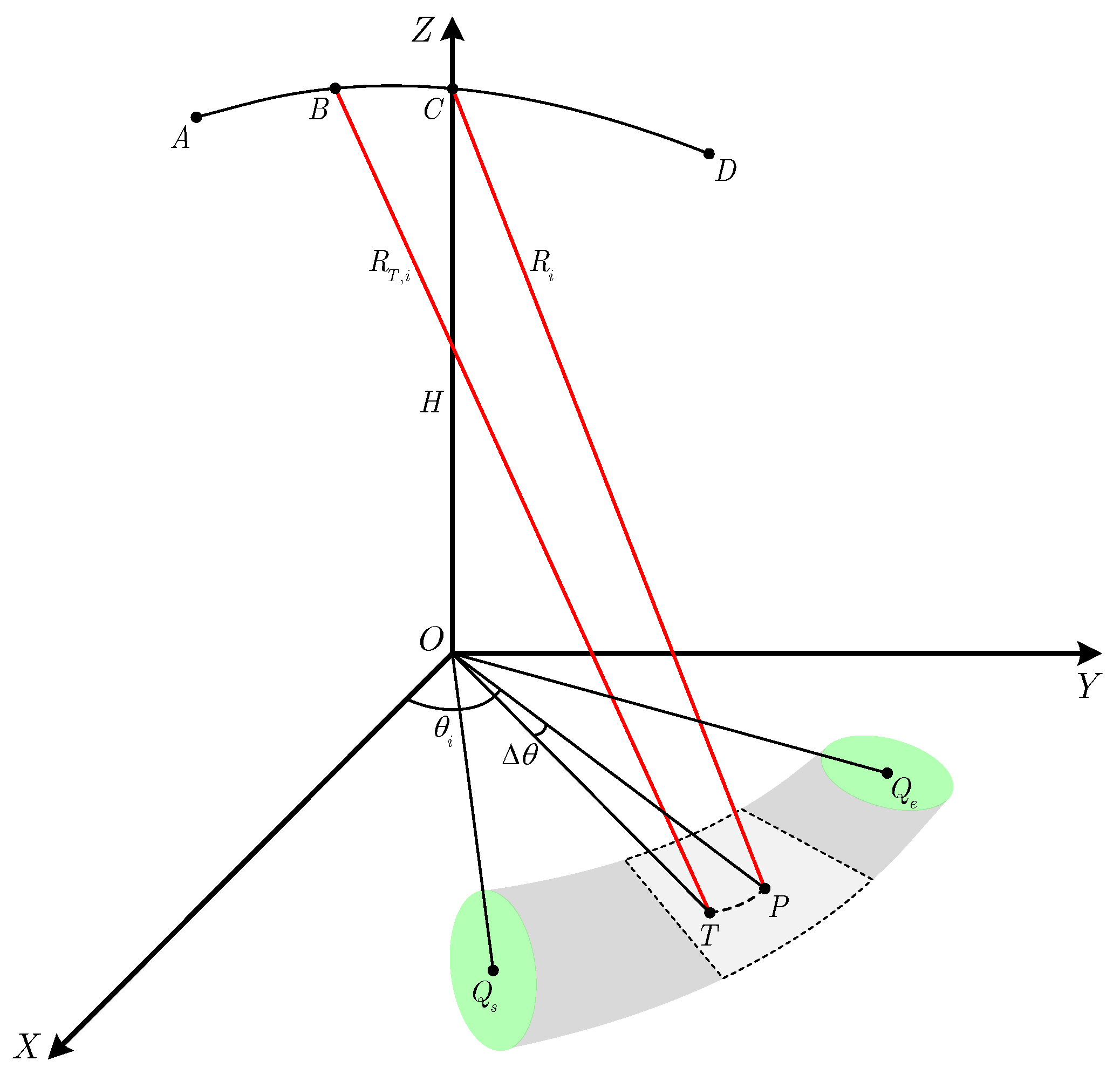
The imaging geometry of maneuvering platform SAR with squint TOPS mode is shown in Figure 1. The platform moves along the curve with velocity vector while the beam is scanning from to with a constant angular speed . is an arbitrary point on the flight track corresponding to azimuth tine . is the platform position at azimuth time . During the following imaging processing, the signal spectrum is divided into several blocks corresponding to different angular areas. is an arbitrary target within the angular area whose center yaw angle is . According to the local polar format definition in [14], the reference range of is . So, the slant range of can be expressed as
where is the nth-order deviation at corresponding to angular area . In each angular area , an arbitrary target can be expressed with the reference range and an angular deviation . The slant range terms are space-variant with and which are the range and azimuth space-variation, respectively. The range-variation can be overcome by range blocking and chirp scaling methods [19]. For azimuth processing, more accurate phase compensations are needed, especially for the Doppler parameters.
2.2. Space-Variation of Doppler Parematers
The azimuthal space-variation of slant range terms in (1) need to be considered in the following processing. are expanded at as
where . is the linear term which will affect the azimuth focusing position. It is also the main component of RCM. is the Doppler chirp rate term which directly affect the azimuth focusing quality. and are higher order terms. They usually affect the sidelobe level of a focused point. There are approximation errors in (2) when calculating the slant range terms. The corresponding phase errors can be expressed as
Some simulations are made to calculate the approximation errors with the system parameters in Table 1.
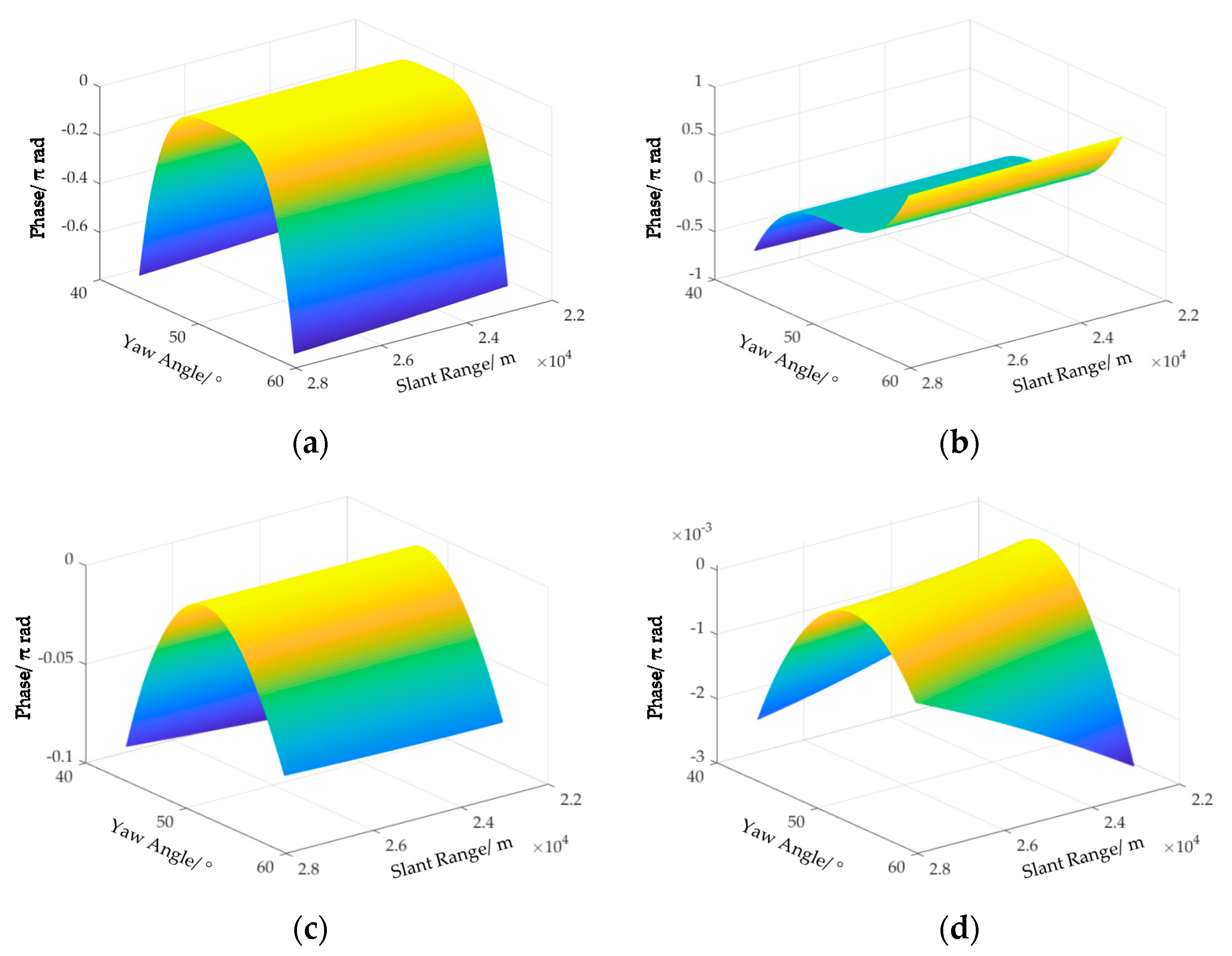
As the simulation results shown in Figure 2, the approximation errors in and can be neglected, for the maximum phase error is less than . However, the expressions for and are not accurate enough, as shown in Figure 2a,b. In order to overcome this problem, angular division is used during the range cell migration correction (RCMC) and azimuth focusing. By dividing the whole steering angle into three parts, the approximation errors can be significantly reduced. As the simulation results shown in Figure 3, the approximation errors of and have been decreased to a value much less than . So, the expressions in (2) are accurate enough for the following signal processing based on the angular division method.
Another advantage of the angular division method is the space-variation of can also be neglected. For the existed space-variation correction methods [10,14], the space-variation of and cannot be removed at the same time. Usually only the space-variation of is compensated. However, to get a well-focused image, the space-variation of also needs to be considered. As the simulation results shown in Figure 4a, the variation cannot be neglected, for the maximum phase value is greater than . After angular division method, the space-variation can be neglected as the results shown in Figure 4b. Furthermore, there is no need for the azimuth signal combination. Therefore, the data of different angular blocks can be processed in parallel.
3. Imaging Algorithm
In this section, an imaging algorithm based on angular division is proposed. Figure 5 shows the flow charts of the algorithm. The SAR data is first multiplied by the unified RWC and nonlinear derotation function. Then, the signal is unambiguous in Doppler. After zero-padding and phase compensation, the signal is recovered in both time and Doppler domain. The signal is divided into several blocks in Doppler according to the angular division. For angular data block i, the data is compensated by the residual RWC function. The space-variant RCM components are removed by KT. The RCM is then corrected by a unified function. For the azimuth focusing, frequency perturbation terms are introduced to correct the space-variant Doppler chirp rate. All the focusing parameters are calculated according to the scene center of each angular block and the data can be processed in parallel. Each angular block i is focused in range-Doppler domain. The final focused SAR image can be obtained by the combination of all the angular block images after geometric correction.
3.1. Spectrum Recovering and Angular Division
By a range Fourier transform, the signal in range frequency domain can be expressed as
where is the range envelop function in frequency domain. is the azimuth beam window. is the range-azimuth coupling phase term which can be expressed as
where is the slant range in (1) without angular division. The corresponding coefficients are and .
The spectrum bandwidth of the TOPS SAR echo signal is constructed by two parts, the resolution bandwidth and the beam steering bandwidth. As the time-frequency diagram shown in Figure 6a, the resolution bandwidth is much smaller than the bandwidth caused by beam steering. The total Doppler bandwidth is much larger than the system PRF which will lead to Doppler ambiguity. The time-frequency line of beam steering can be calculated by
where is corresponding to the slope of time-frequency line. is the Doppler deviation caused by squint mode. It can be removed by unified RWC and range compression. The compensation function can be derived as
is the linear component caused by beam steering. Usually, this term can be compensated by linear derotation [17], as shown in Figure 6b. However, by nonlinear derotation, the required system PRF can be further reduced. The compensation function can be formed as
(7) and (8) are both calculated with reference to the scene center corresponding to . The time-frequency diagram of signal after nonlinear derotation is shown in Figure 6c. The time-frequency line in (6) becomes
where is the residual component after nonlinear derotation.
It can be noticed that the signal is unambiguous in Doppler. Thus, the Doppler interval can be extended by zero-padding after an azimuth Fourier transform. In order to get the numbers of zero-padding, the Doppler bandwidth of echo signal and signal after nonlinear derotation need to be calculated. According to (6), the Doppler bandwidth can be derived as the beam steering bandwidth:
Similarly, the signal Doppler bandwidth in Figure 6c can be expressed as
So, the number of zero-padding can be derived with considering the sampling redundancy:
Furthermore, the azimuth sampling frequency has been extended as
The new azimuth time and frequency have changed to and , respectively.
Then, the signal is transformed into azimuth time domain. A phase function is needed to compensate the influence caused by the nonlinear derotation in (8). The function can be formed as
After phase compensation, the signal is unambiguous in Doppler, as shown in Figure 6d.
Then, the signal can be divided into several blocks in Doppler according to the angular division. As shown in Figure 7a, the observation area is divided uniformly into n blocks. Each block has a same yaw angle. There is a mapping relation between the yaw angle and the Doppler, as shown in Figure 7b. For block i, the corresponding support region in Doppler can be easily found. To avoid resolution loss in the margin area, the selected data support region in Doppler is a bit larger than the calculated one. So, there is no need for the signal to be recombined before azimuth focusing. The signal after angular division can be processed in parallel without resolution loss.
3.2. Residual RWC and Space-Variant RCMC
After angular division and aforementioned processing steps, the phase in (5) becomes
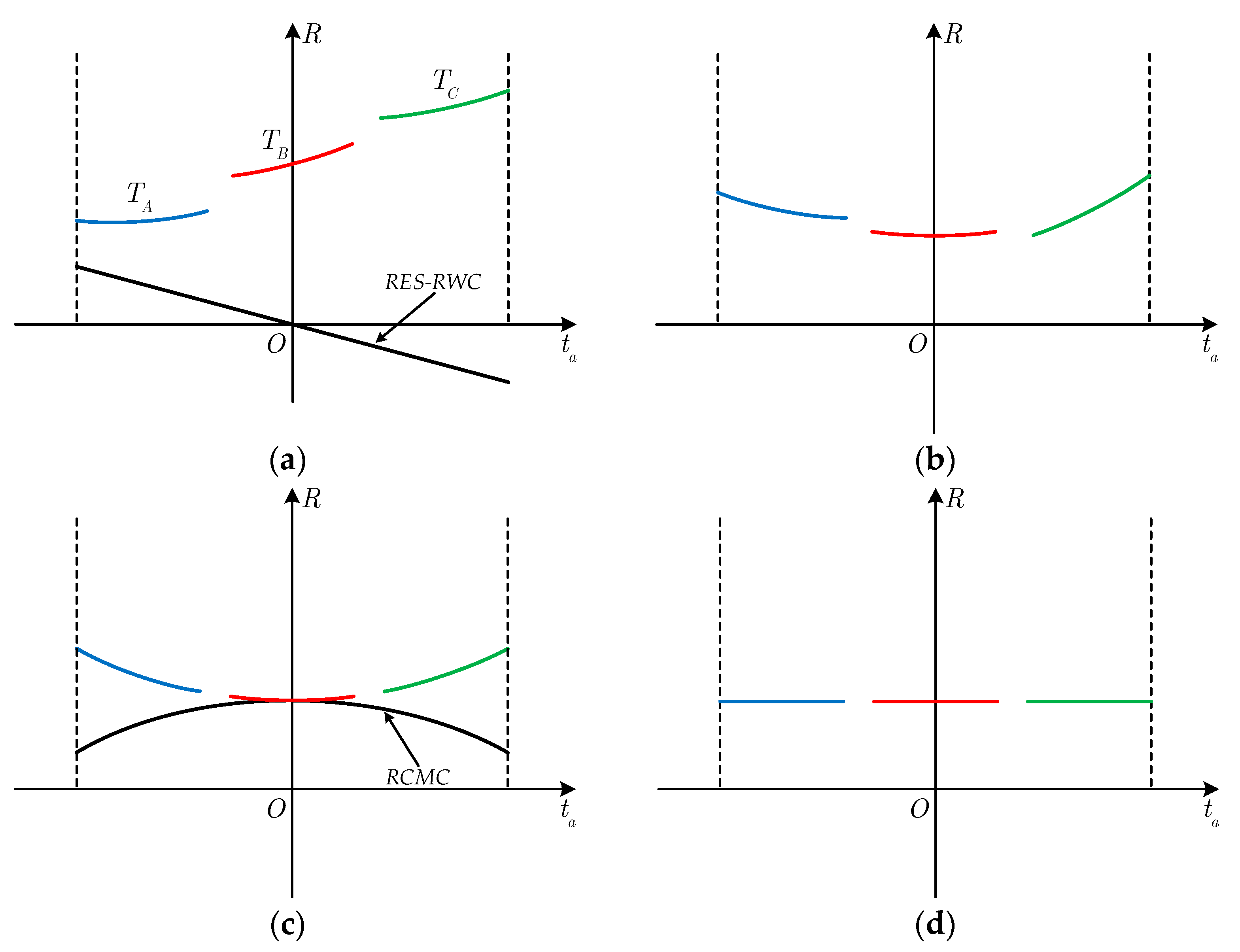
According to the simulation results in Figure 2 and Figure 4, the third and the fourth order terms are processed as constant components. is the residual linear component after the unified RWC in Equation (7). Figure 8 shows the RCM lines of targets , and which share a same reference range. There are still residual RWC components, as shown in Figure 8a. The signal after angular division needs to be processed with reference to the scene center of each angular block. So, the residual RWC need to be compensated by the function:
Then, the linear term becomes . It can be noticed that there are still space-variant terms remained. As shown in Figure 8b, the RCM lines of and cannot be corrected by a same function with reference to . In order to remove the space-variant components, KT is applied by interpolating the signal into a new time interval. The mapping relation can be expressed as
where is the azimuth time after KT. The corresponding azimuth frequency is . After KT, the phase terms in (15) becomes
where
is the coupling phase term which can be decomposed into three terms. is the RCM component. is the secondary range compression (SRC) term which is caused by the KT. is the azimuth phase term. It can be noticed that the linear RCM term including the space-variant components have been removed. The remained RCM and SRC terms can be compensated with reference to the scene center of each angular block. The compensation function can be formed as
After RCM and SRC compensation and a range inverse Fourier transform, the signal can be expressed as
It can be seen in (23) that the targets sharing a same reference range have been focused into a same range cell. There is no mismatch between the range focused position and the azimuth phase [10] which is an advantage over the conventional RWC based methods.
3.3. Aizmuth Fousing
The phase terms in (21) are space-variant with the . is the Doppler chirp rate term which will directly affect the azimuth focusing quality. Figure 9 shows the time-frequency lines of targets , and which are in a same range cell. The slope of the time-frequency line mainly corresponding to the Doppler chirp rate which are , and . In order to remove the space-variation of Doppler chirp rate, frequency perturbation terms are introduced. By an azimuth Fourier transform, the signal is transformed into Doppler domain:
where is the residual Doppler center after residual RWC of block i. The constant phase term in (24) is neglected, for it has no influence on the azimuth focusing. can be expressed as
By introducing the frequency perturbation terms, the space-variation of can be removed in time domain. The perturbation function can be formed as
where and are coefficients to be determined. Multiplying (26) with (24), the signal is then transformed into azimuth time domain:
where is the coefficients after frequency perturbation which can be expressed as:
The space-variation of and are neglected for the perturbation terms are small. For further analysis, is expanded as Taylor series at . The first and second order coefficients can be derived as
To remove the space-variant terms, and are set to be zero. So and can be derived as
After the frequency perturbation, the Doppler chirp rate of targets with same reference range are corrected to a same value, as shown in Figure 9b. Then, they can be compensated by a unified deramp function which can be formed as
The deramp function is derived according to the constant parts of , and in (28). After deramp operation, the time-frequency lines are compensated to be perpendicular to the axis, as shown in Figure 9c. Finally, by an azimuth Fourier transform, the 2-D focused image can be obtained as
3.4. Geometric Correction
The image of each angular block is focused in range-Doppler domain, as derived in (32). There is geometric distortion in azimuth. According to (28), the Doppler focused position is modulated by , and . Assuming an arbitrary target in an angular block with coordinate . The corresponding yaw angle can be calculated as . Comparing with of each block, the block number of the target can be found. So, the reference range and angular deviation of target in block i can be derived as
The signal is divided in Doppler according to the angular division. Thus, there are some overlaps of different data blocks in Doppler. The final SAR image can be obtained by the direct combination of all angular block images.
4. Experimental Results
In this part, some experiments are made based on the parameters in Table 1 and the geometry in Figure 10. The key processing steps have been verified as follows.
4.1. Correction of Space-Variant RCM
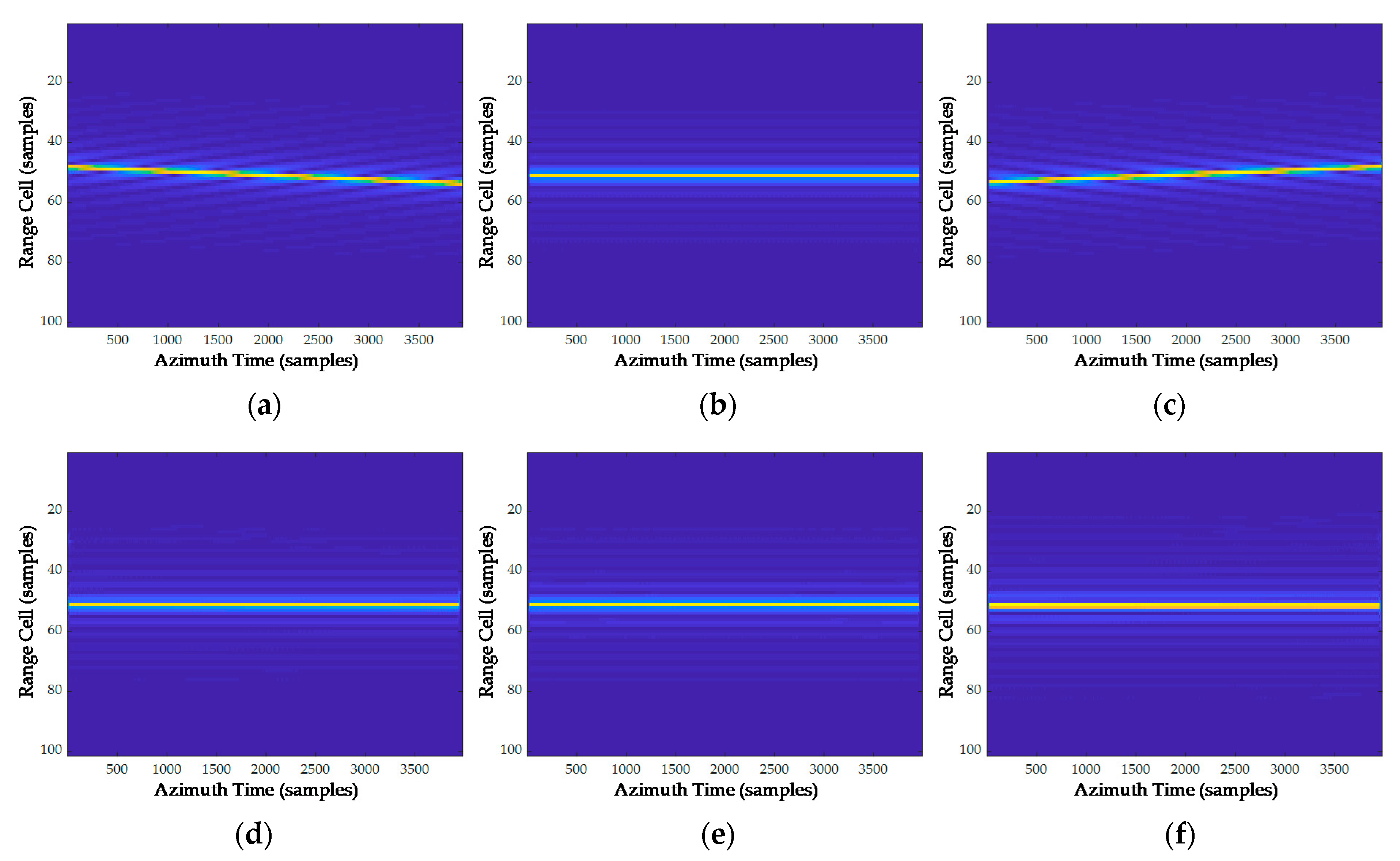
In order to verify the method of space-variant RCMC, several targets with different reference range are selected. The target distribution geometry is shown in Figure 10a. Target , and are located at near, center and far reference ranges, respectively. Then, two different RCMC methods are used. The simulation results are shown in Figure 11. By time domain RCMC without KT, there are still space-variant RCM components remained. It can be noticed in Figure 11a,c that the residual RCM is much larger than a range cell. By the proposed RCMC method, the space-variant RCM can be fully removed. The RCM can be accurately compensated, as shown in Figure 11d,f.
4.2. Performance of Geometric Correction and Azimuth Focusing
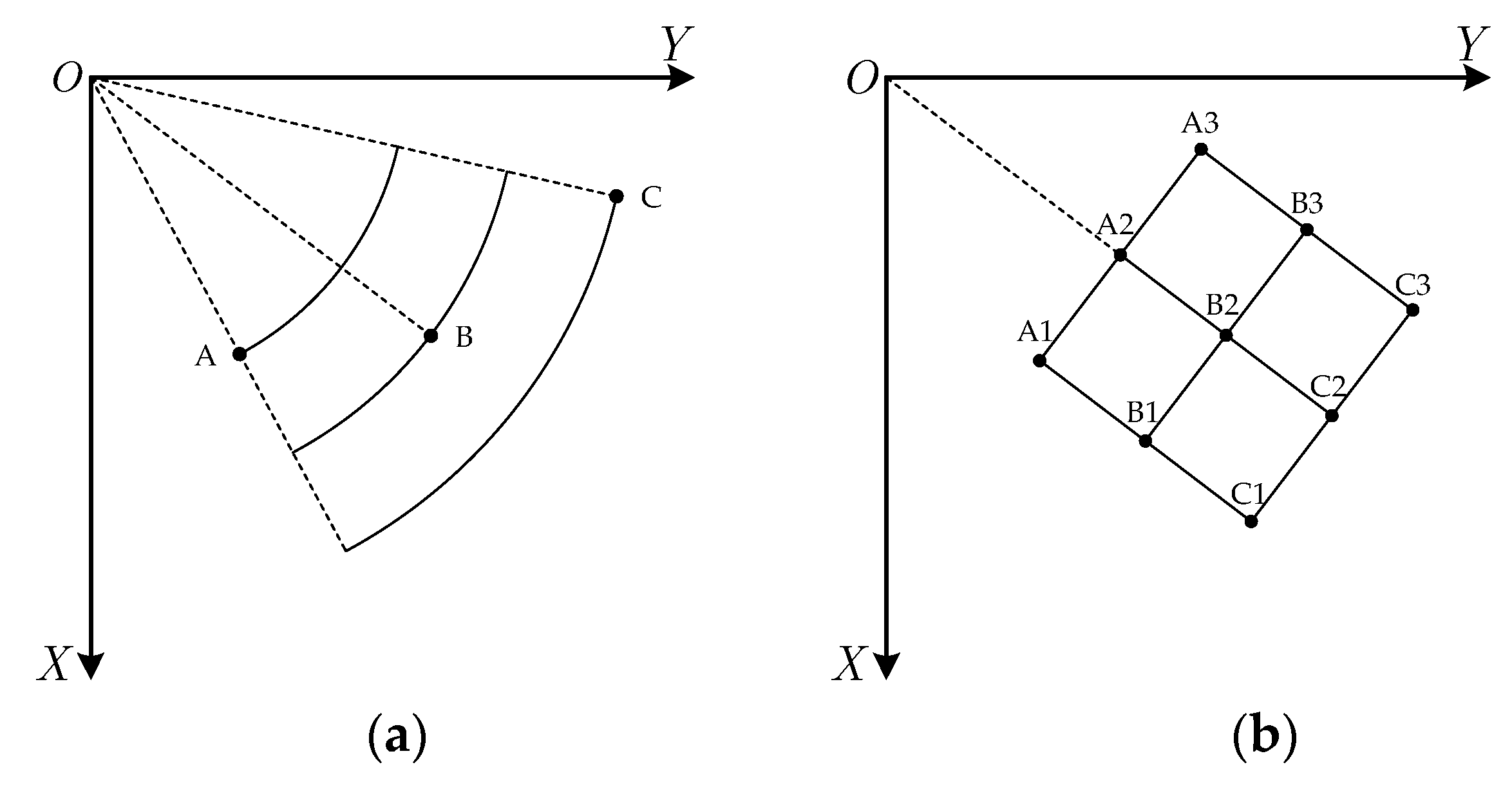
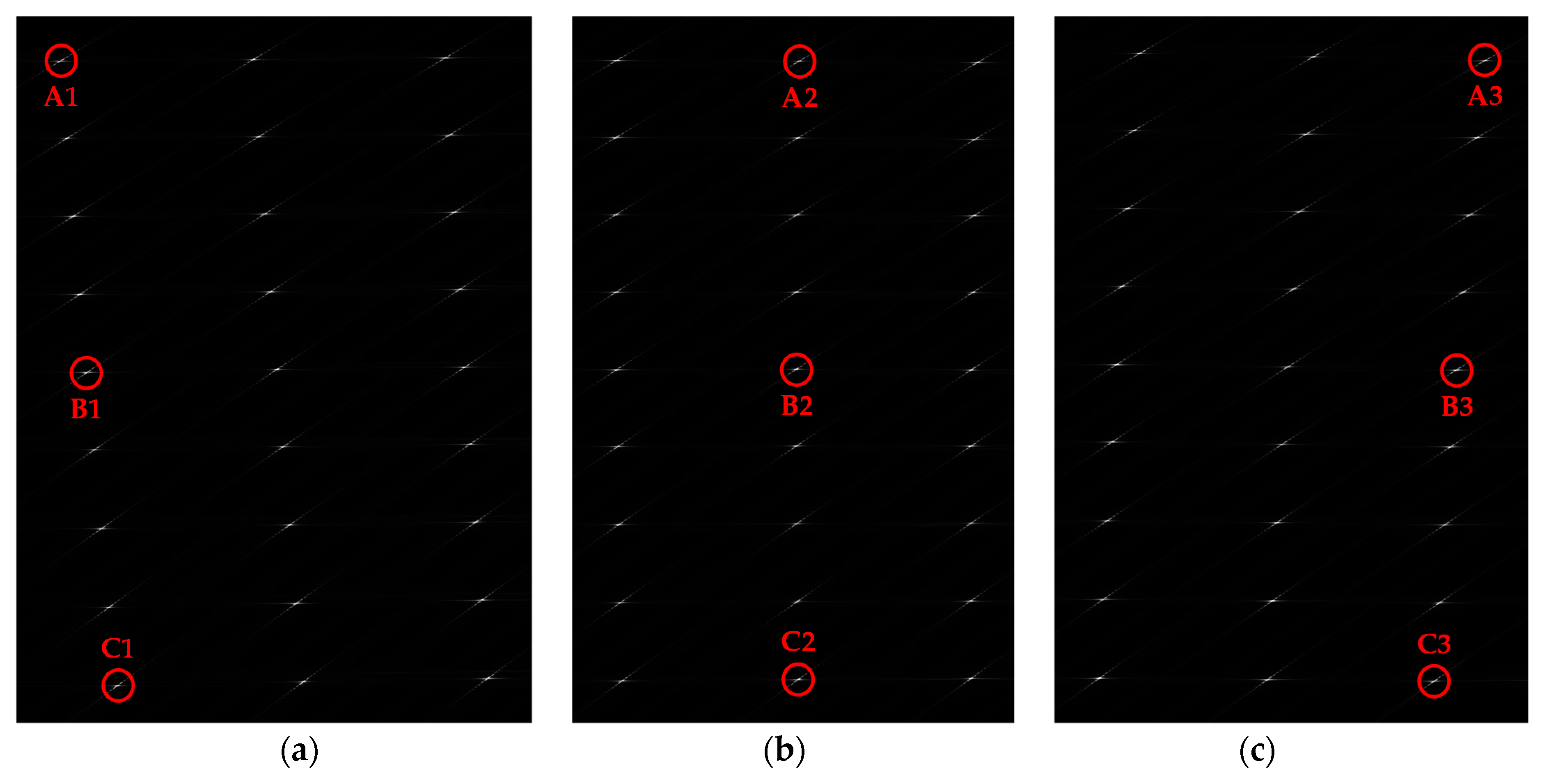
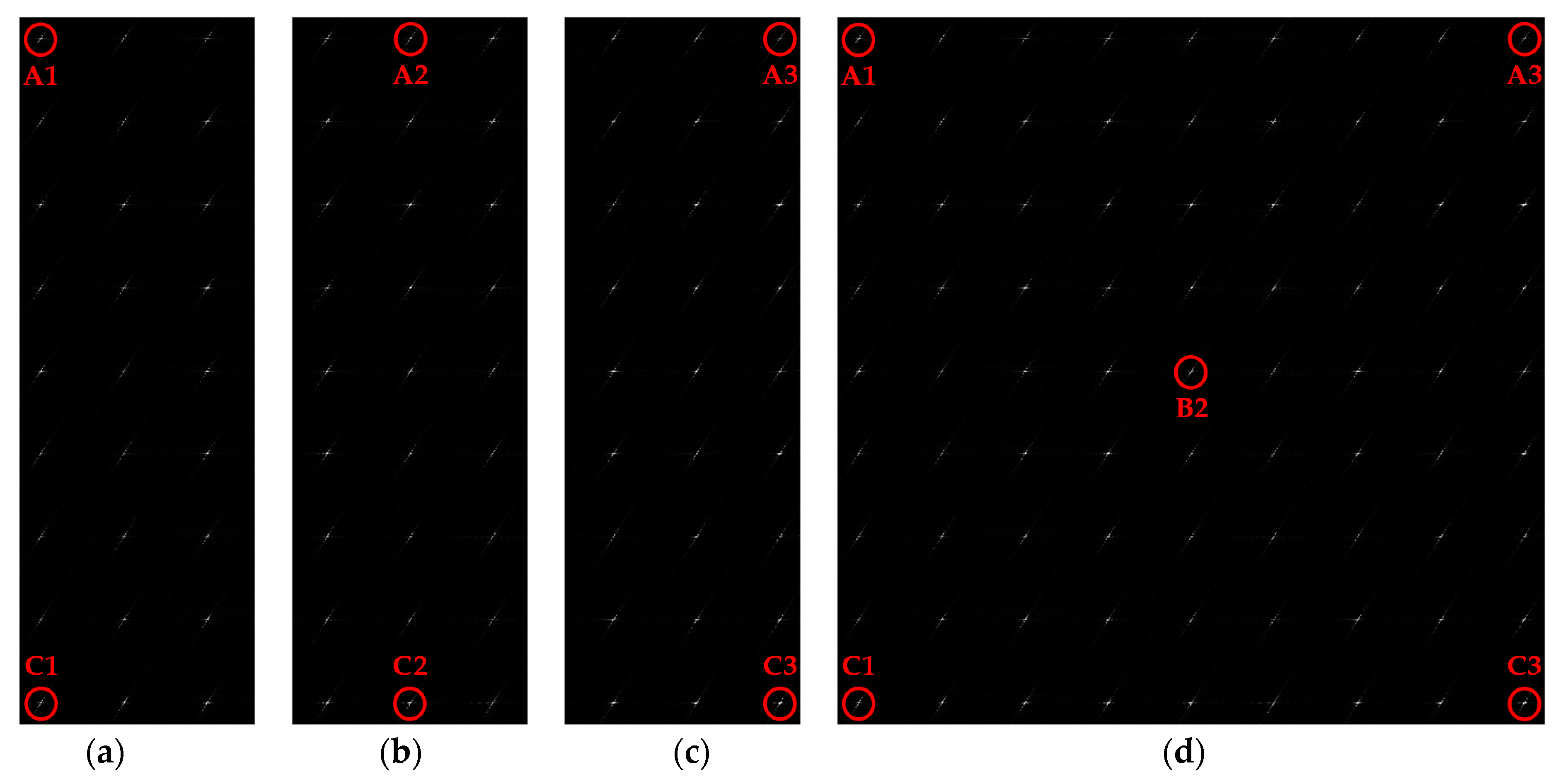
To verify the effectiveness of geometric correction, 9 × 9-point targets matrix with a distribution area of 5 km × 5 km are used. Nine targets are selected and the distribution geometry is shown in Figure 10b. By dividing the targets into three angular blocks, the imaging results are shown in Figure 12. Because the azimuth focusing position is modulated by the frequency perturbation terms, there is obvious geometric distortion in each angular block image. The geometric correction results of angular block images are shown in Figure 13a–c. According to the coordinates of selected targets—A1(26, 26), C1(2526, 26), A2(26, 426), C2(2526, 426), A3(26, 826) and C3(2526, 826)—the geometry distortion within each block has been corrected. By directly combining the angular block images, the final focused image can be obtained, as shown in Figure 13d. To check the image distortion in the final image, targets A1, C1, B2, C1 and C3 are selected in Figure 12. Their locations in Figure 13d are (26, 26), (2526, 26), (1276, 1276), (26, 2526) and (2526, 2526). The resolution cell of the interpolated image in Figure 13 are 2 m × 2 m. It can be found that the geometric distortion is controlled within one resolution cell.
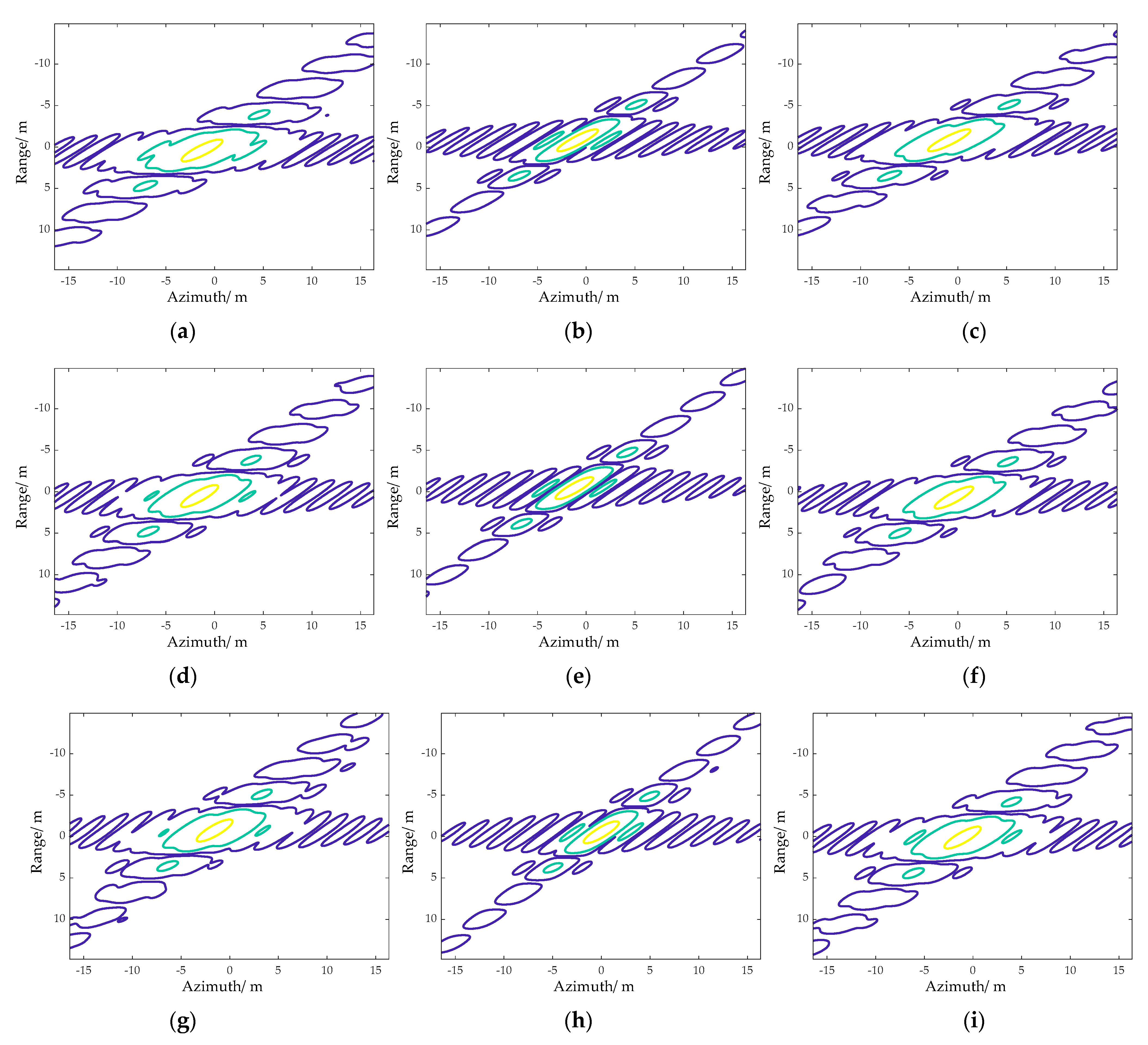
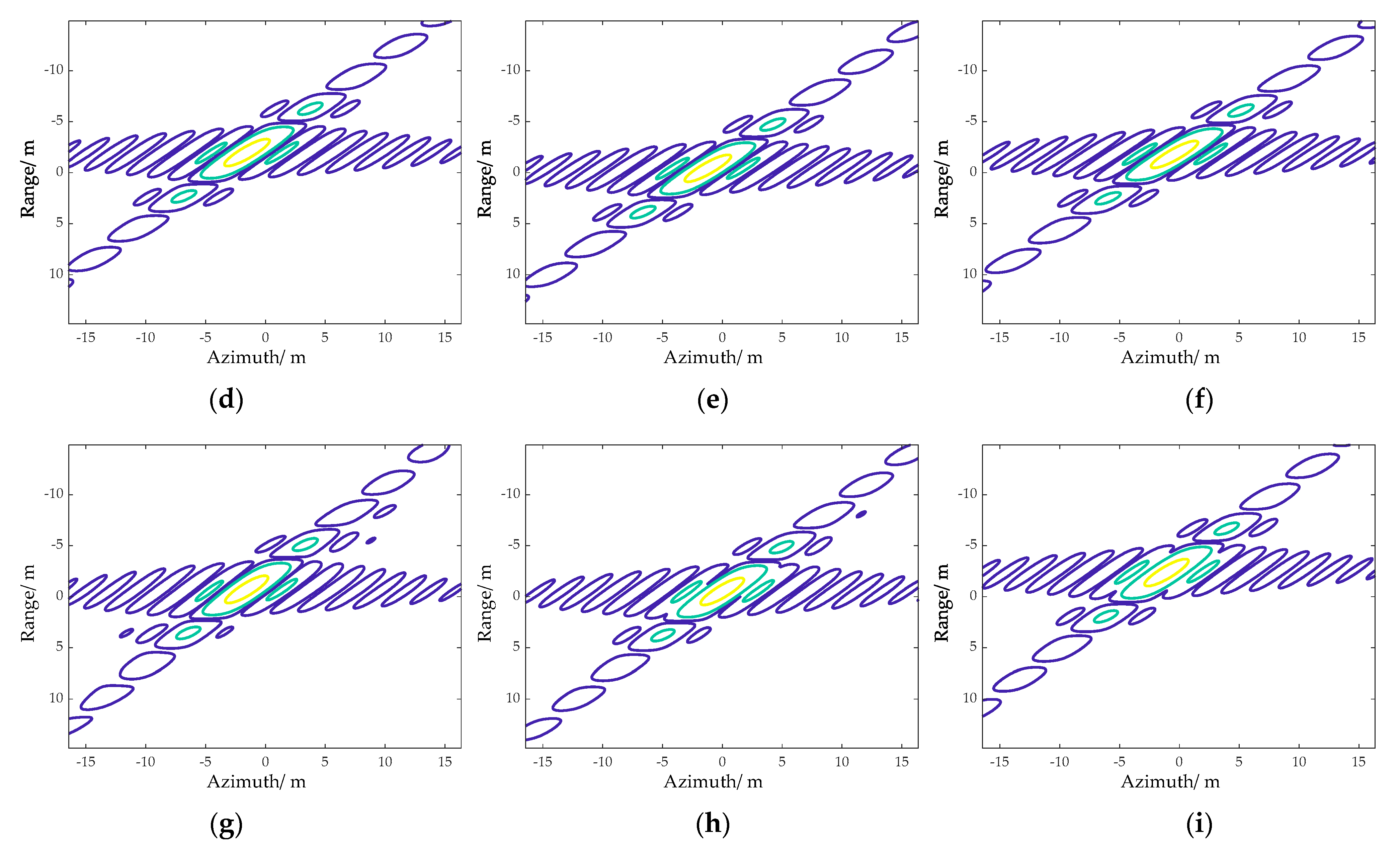
A comparison is made to verify the effectiveness of the proposed method. The method in [10] is chosen as a reference. Considering the method is not designed to process TOPS SAR data. Processing steps of the proposed methods are used except the signal model. By the reference method, the signal model is low accurate after variable substitution. To evaluate the focusing performance, 2-D contour images of nine targets selected in Figure 10 are shown in Figure 14 and Figure 15. Like the contour images in [28], the 2-D resolution is visible from the figure. The space-variant components of the third-order term are still remained. This will lead to azimuth defocusing in edge area, as shown in Figure 14. Compared with the reference method, the proposed range model can be directly matched with the signal after RWC which is more accurate than the reference one. The variation of the third-order phase term can be compensated as constant term within each angular block. So, the azimuth focusing performance can be improved, as shown in Figure 15. Furthermore, the 2-D PSLR, ISLR and IRW of these targets processed by the two methods are calculated, as listed in Table 2 and Table 3.
5. Discussion
This paper is based on previous works [14]. It provides another solution for high-speed maneuvering SAR imaging in TOPS mode. For the focusing performance, methods proposed in the two papers are in a same category. However, several main procedures are different: the preprocessing steps and the processing architecture. Signal ambiguity in Doppler is a feature of TOPS SAR data. The preprocessing steps in [14] is designed with reference to the methods in [16,17]. The key idea is to extend the data support region in Doppler by sacrificing that in azimuth time. It causes extra processing complexity when performing KT and other time domain compensations. For the method in this paper, the signal is unambiguous both in azimuth time and Doppler. So, the compensation functions can be easily applied without restrictions. A disadvantage is that the zero-padding increases the computational complexity. Thus, the parallel processing architecture is used to accelerate the data processing. It also has the potential ability to achieve higher focusing performance when the azimuth swath is larger.
6. Conclusions
This paper proposed an imaging algorithm for high-speed maneuvering platform SAR with squint TOPS mode. The range model is formed in local polar format which can overcome the mismatch between the range model and the signal after RWC. The Doppler folded signal is recovered by nonlinear derotation and zero-padding. The signal is then divided into several blocks according to the angular block division and can be processed in parallel. By KT, the space-variant RCM components are removed. Then, frequency perturbation terms are introduced to compensate the Doppler chirp rate variation. The focusing parameters are calculated according to the scene center of each angular block. Finally, the geometric distortion of each angular block is corrected by 2-D interpolation. The final focused image can be obtained by directly combining all the angular block images. Simulated SAR data has verified the effectiveness of the proposed algorithm.
Author Contributions
Conceptualization, B.B. and G.S.; methodology, B.B.; software, B.B.; validation, Y.Q. and M.X.; formal analysis, K.X.; investigation, B.B.; resources, B.B.; data curation, B.B.; writing—original draft preparation, B.B.; writing—review and editing, K.X.; visualization, B.B.; supervision, Y.Q.; project administration, M.X.; funding acquisition, B.B. All authors have read and agreed to the published version of the manuscript.
Funding
This work was partially supported by National Natural Science Foundation of China (62001353, 62101400), China Postdoctoral Science Foundation (2020M673345) and the Fundamental Research Funds for the Central Universities (XJS200202).
Data Availability Statement
The data is available to readers by contacting the corresponding author.
Acknowledgments
The author would like to thank the Institute of Advanced Remote Sensing technology.
Conflicts of Interest
The authors declare no conflict of interest.
References
- Moreira, A.; Prats-Iraola, P.; Younis, M.; Krieger, G.; Hajnsek, I.; Papathanassiou, K.P. A tutorial on synthetic aperture radar. IEEE Geosci. Remote Sens. Mag. 2013, 1, 6–43. [Google Scholar] [CrossRef] [Green Version]
- Moreira, A.; Krieger, G.; Hajnsek, I.; Papathanassiou, K.; Younis, M.; Lopez-Dekker, P.; Huber, S.; Villano, M.; Pardini, M. Tandem-L: A highly innovative bistatic SAR mission for global observation of dynamic processes on the earth’s surface. IEEE Geosci. Remote Sens. Mag. 2015, 3, 8–23. [Google Scholar] [CrossRef]
- Carrara, W.G.; Goodman, R.S.; Majewski, R.M. Spotlight Synthetic Radar: Signal Processing Algorithm; Artech House: Boston, MA, USA, 1995. [Google Scholar]
- Cumming, I.G.; Wong, F. Digital Processing of Synthetic Aperture Radar Data: Algorithms and Implementation; Artech House: Norwood, MA, USA, 2005. [Google Scholar]
- Zhang, L.; Qiao, Z.; Xing, M.D.; Yang, L.; Bao, Z. A robust motion compensation approach for UAV SAR imagery. IEEE Trans. Geosci. Remote Sens. 2012, 50, 3202–3218. [Google Scholar] [CrossRef]
- Zhang, L.; Sheng, J.; Xing, M.; Qiao, Z.; Xiong, T.; Bao, Z. Wavenumber-domain autofocusing for highly squinted UAV SAR imagery. IEEE Sens. J. 2011, 12, 1574–1588. [Google Scholar] [CrossRef]
- Wang, G.; Zhang, M.; Huang, Y.; Zhang, L.; Wang, F. Robust two-dimensional spatial-variant map-drift algorithm for UAV SAR autofocusing. Remote Sens. 2019, 11, 340. [Google Scholar] [CrossRef] [Green Version]
- Tang, S.; Zhang, L.; So, H.C. Focusing high-resolution highly-squinted airborne SAR data with maneuvers. Remote Sens. 2018, 10, 862. [Google Scholar] [CrossRef] [Green Version]
- Tang, S.; Zhang, L.; Guo, P.; Liu, G.; Sun, G.C. Acceleration model analyses and imaging algorithm for highly squinted airborne spotlight-Mode SAR with maneuvers. IEEE J. Sel. Topics Appl. Earth Observ. Remote Sens. 2015, 8, 1120–1131. [Google Scholar] [CrossRef]
- Li, Z.; Xing, M.; Liang, Y.; Gao, Y.; Chen, J.; Huai, Y.; Zeng, L.; Sun, G.-C.; Bao, Z. A frequency-domain imaging algorithm for highly squinted SAR mounted on maneuvering platforms with nonlinear trajectory. IEEE Trans. Geosci. Remote Sens. 2016, 54, 4023–4038. [Google Scholar] [CrossRef]
- Zeng, T.; Li, Y.; Ding, Z. Subaperture approach based on azimuth-dependent range cell migration correction and azimuth focusing parameter equalization for maneuvering high-squint-mode SAR. IEEE Trans. Geosci. Remote Sens. 2015, 52, 6718–6734. [Google Scholar] [CrossRef]
- Sun, G.-C.; Xing, M.; Xia, X.-G.; Wu, Y.; Huang, P.; Wu, Y.; Bao, Z. Multichannel full-aperture azimuth processing for beam steering SAR. IEEE Trans. Geosci. Remote Sens. 2013, 51, 4761–4778. [Google Scholar] [CrossRef]
- Wu, Y.; Sun, G.-C.; Xia, X.-G.; Xing, M.; Yang, J.; Bao, Z. An azimuth frequency non-linear chirp scaling (FNCS) algorithm for TOPS SAR imaging with high squint angle. IEEE J. Sel. Top. Appl. Earth Obs. Remote Sens. 2013, 7, 213–221. [Google Scholar] [CrossRef]
- Bie, B.; Sun, G.; Xia, X.; Xing, M.; Guo, L.; Bao, Z. High-speed maneuvering platforms squint beam-steering SAR imaging without sub-aperture. IEEE Trans. Geosci. Remote Sens. 2019, 57, 6974–6985. [Google Scholar] [CrossRef]
- Ran, L.; Liu, Z.; Xie, R.; Zhang, L. Focusing high-squint synthetic aperture radar data based on factorized back-projection and precise spectrum fusion. Remote Sens. 2019, 11, 2885. [Google Scholar] [CrossRef] [Green Version]
- Yang, J.; Sun, G.-C.; Xing, M.; Xia, X.-G.; Liang, Y.; Bao, Z. Squinted TOPS SAR imaging based on modified range migration algorithm and spectral analysis. IEEE Geosci. Remote Sens. Lett. 2014, 11, 1707–1711. [Google Scholar] [CrossRef]
- Prats, P.; Scheiber, R.; Mittermayer, J.; Meta, A.; Moreira, A. Processing of sliding spotlight and TOPS SAR data using baseband azimuth scaling. IEEE Trans. Geosci. Remote Sens. 2010, 48, 770–780. [Google Scholar] [CrossRef] [Green Version]
- Engen, G.; Larsen, Y. Efficient full aperture processing of TOPS mode data using the moving band chirp Z-transform. IEEE Trans. Geosci. Remote Sens. 2011, 49, 3688–3693. [Google Scholar] [CrossRef]
- Raney, R.K.; Runge, H.; Bamler, R.; Cumming, I.G.; Wong, F.H. Precision SAR processing using chirp scaling. IEEE Trans. Geosci. Remote Sens. 1994, 32, 786–799. [Google Scholar] [CrossRef]
- Sun, G.; Xing, M.; Wang, Y.; Yang, J.; Bao, Z. A 2-D space-variant chirp scaling algorithm based on the RCM equalization and sub-band synthesis to process geosynchronous SAR data. IEEE Trans. Geosci. Remote Sens. 2014, 52, 4868–4880. [Google Scholar]
- Wong, F.H.; Yeo, T.S. New applications of nonlinear chirp scaling in SAR data processing. IEEE Trans. Geosci. Remote Sens. 2001, 39, 946–953. [Google Scholar] [CrossRef]
- Wong, F.H.; Cumming, I.G.; Neo, Y.L. Focusing bistatic SAR data using the nonlinear chirp scaling. IEEE Trans. Geosci. Remote Sens. 2008, 46, 2493–2505. [Google Scholar] [CrossRef] [Green Version]
- Sun, G.; Xing, M.; Liu, Y.; Sun, L.; Bao, Z.; Wu, Y. Extended NCS based on method of series reversion for imaging of highly squinted SAR. IEEE Geosci. Remote Sens. Lett. 2011, 8, 446–450. [Google Scholar] [CrossRef]
- Sun, G.; Jiang, X.; Xing, M.; Qiao, Z.-J.; Wu, Y.; Bao, Z. Focus improvement of highly squinted data based on azimuth nonlinear scaling. IEEE Trans. Geosci. Remote Sens. 2011, 49, 2308–2322. [Google Scholar] [CrossRef]
- An, D.; Huang, X.; Jin, T.; Zhou, Z. Extended nonlinear chirp scaling algorithm for high-resolution highly squint SAR data focusing. IEEE Trans. Geosci. Remote Sens. 2012, 50, 3595–3609. [Google Scholar] [CrossRef]
- Li, N.; Bie, B.; Sun, G.C.; Xing, M.; Bao, Z. A high-squint TOPS SAR imaging algorithm for maneuvering platforms based on joint time-doppler deramp without subaperture. IEEE Geosci. Remote Sens. Lett. 2020, 17, 1899–1903. [Google Scholar] [CrossRef]
- Xing, M.; Wu, Y.; Zhang, Y.D.; Sun, G.-C.; Bao, Z. Azimuth resampling processing for highly squinted synthetic aperture radar imaging with several modes. IEEE Trans. Geosci. Remote Sens. 2014, 52, 4339–4352. [Google Scholar] [CrossRef]
- Prats-Iraola, P.; Scheiber, R.; Rodriguez-Cassola, M.; Mittermayer, J.; Wollstadt, S.; De Zan, F.; Brautigam, B.; Schwerdt, M.; Reigber, A.; Moreira, A. On the processing of very high resolution spaceborne SAR data. IEEE Trans. Geosci. Remote Sens. 2014, 52, 6003–6016. [Google Scholar] [CrossRef] [Green Version]
Figure 1.
Imaging geometry of maneuvering platform SAR with TOPS mode.

Figure 2.
Approximation phase errors of slant range terms before angular division. (a) The first-order term. (b) The second-order term. (c) The third-order term. (d) The fourth-order term.
Figure 2.
Approximation phase errors of slant range terms before angular division. (a) The first-order term. (b) The second-order term. (c) The third-order term. (d) The fourth-order term.

Figure 3.
Approximation phase errors of slant range terms after angular division. (a) The first-order term. (b) The second-order term.
Figure 3.
Approximation phase errors of slant range terms after angular division. (a) The first-order term. (b) The second-order term.

Figure 4.
Phase of the space-variant third-order slant range term. (a) The space-variant phase before angular division. (b) The space-variant phase after angular division.
Figure 4.
Phase of the space-variant third-order slant range term. (a) The space-variant phase before angular division. (b) The space-variant phase after angular division.

Figure 5.
Flow chart of the proposed algorithm.

Figure 6.
Spectrum recovering analysis by the time-frequency diagrams. (a) Echo signal. (b) Signal after RWC and linear derotation. (c) Signal after nonlinear derotation and zero-padding. (d) Recovered signal.
Figure 6.
Spectrum recovering analysis by the time-frequency diagrams. (a) Echo signal. (b) Signal after RWC and linear derotation. (c) Signal after nonlinear derotation and zero-padding. (d) Recovered signal.

Figure 7.
Angular division analysis. (a) Block division in angular domain. (b) Mapping relation between yaw angle and Doppler.
Figure 7.
Angular division analysis. (a) Block division in angular domain. (b) Mapping relation between yaw angle and Doppler.

Figure 8.
RCM lines of targets shared a same reference range. (a) RCM lines after unified RWC. (b) RCM lines after residual RWC. (c) RCM lines after KT. (d) RCM lines after RCMC.
Figure 8.
RCM lines of targets shared a same reference range. (a) RCM lines after unified RWC. (b) RCM lines after residual RWC. (c) RCM lines after KT. (d) RCM lines after RCMC.

Figure 9.
Azimuth focusing analysis of targets sharing a same reference range. (a) Time-frequency lines of targets with different Doppler chirp rate. (b) Time-frequency lines after frequency perturbation. (c) Time-frequency lines after deramp. (d) Azimuth focused in Doppler domain.
Figure 9.
Azimuth focusing analysis of targets sharing a same reference range. (a) Time-frequency lines of targets with different Doppler chirp rate. (b) Time-frequency lines after frequency perturbation. (c) Time-frequency lines after deramp. (d) Azimuth focused in Doppler domain.

Figure 10.
Simulation geometry. (a) Point targets in polar format. (b) Point targets matrix.

Figure 11.
RCM lines of targets in Figure 10a. (a) RCM line of target A without KT. (b) RCM line of target B without KT. (c) RCM line of C without KT. (d) RCM line of target A with KT. (e) RCM line of target B with KT. (f) RCM line of target C with KT.
Figure 11.
RCM lines of targets in Figure 10a. (a) RCM line of target A without KT. (b) RCM line of target B without KT. (c) RCM line of C without KT. (d) RCM line of target A with KT. (e) RCM line of target B with KT. (f) RCM line of target C with KT.

Figure 12.
Imaging results of different angular blocks. (a) The image of angular block 1. (b) The image of angular block 2. (c) The image of angular block 3.
Figure 12.
Imaging results of different angular blocks. (a) The image of angular block 1. (b) The image of angular block 2. (c) The image of angular block 3.

Figure 13.
Images after geometric correction. (a) The image of angular block 1. (b) The image of angular block 2. (c) The image of angular block 3. (d) The image after angular blocks combination.
Figure 13.
Images after geometric correction. (a) The image of angular block 1. (b) The image of angular block 2. (c) The image of angular block 3. (d) The image after angular blocks combination.

Figure 14.
Contour images of point targets selected in Figure 12 with contour lines at −3, −15 and −30 dB by the reference method. (a) Contour image of A1. (b) Contour image of A2. (c) Contour image of A3. (d) Contour image of B1. (e) Contour image of B2. (f) Contour image of B3. (g) Contour image of C1. (h) Contour image of C2. (i) Contour image of C3.

Figure 15.
Contour images of point targets selected in Figure 12 with contour lines at −3, −15 and −30 dB by the proposed method. (a) Contour image of A1. (b) Contour image of A2. (c) Contour image of A3. (d) Contour image of B1. (e) Contour image of B2. (f) Contour image of B3. (g) Contour image of C1. (h) Contour image of C2. (i) Contour image of C3.


Table 1.
System parameters.
| Parameters | Value |
|---|---|
| Carrier frequency | 15 GHz |
| Range bandwidth | 50 MHz |
| Pulse width | 10 μs |
| Height | 16.5 km |
| Center slant range | 30 km |
| Center yaw angle | 50° |
| Center squint angle | 39.8° |
| Time duration | 0.6 s |
| Steering angle | 42.13°~57.87° |
| Range swath | 5 km |
| Azimuth swath | 6.88 km |
| (vx, vy, vz) | (−40, 1300, −600) m/s |
| (ax, ay, az) | (−15, −30, −35) m/s2 |
Table 2.
PSLR, ISLR and IRW of selected targets in Figure 10b by the reference method.
Table 2.
PSLR, ISLR and IRW of selected targets in Figure 10b by the reference method.
| Target | Range | Azimuth | ||||
|---|---|---|---|---|---|---|
| PSLR(dB) | ISLR(dB) | IRW(m) | PSLR(dB) | ISLR(dB) | IRW(m) | |
| A1 | −13.26 | −10.97 | 2.68 | −5.74 | −7.02 | 2.18 |
| A2 | −13.23 | −10.98 | 2.68 | −13.10 | −10.52 | 1.85 |
| A3 | −13.21 | −10.92 | 2.68 | −8.48 | −6.59 | 2.01 |
| B1 | −13.23 | −10.98 | 2.68 | −7.65 | −5.89 | 2.01 |
| B2 | −13.14 | −10.89 | 2.67 | −13.24 | −10.70 | 1.89 |
| B3 | −13.24 | −10.97 | 2.68 | −8.43 | −6.34 | 1.97 |
| C1 | −13.19 | −10.95 | 2.68 | −7.37 | −5.73 | 2.06 |
| C2 | −13.18 | −10.97 | 2.68 | −13.21 | −10.65 | 1.85 |
| C3 | −13.25 | −10.96 | 2.68 | −7.04 | −5.28 | 2.10 |
Table 3.
PSLR, ISLR and IRW of selected targets in Figure 10b by the proposed method.
Table 3.
PSLR, ISLR and IRW of selected targets in Figure 10b by the proposed method.
| Target | Range | Azimuth | ||||
|---|---|---|---|---|---|---|
| PSLR(dB) | ISLR(dB) | IRW(m) | PSLR(dB) | ISLR(dB) | IRW(m) | |
| A1 | −13.26 | −10.97 | 2.68 | −12.81 | −10.30 | 1.85 |
| A2 | −13.23 | −10.98 | 2.68 | −13.10 | −10.52 | 1.85 |
| A3 | −13.21 | −10.92 | 2.68 | −13.30 | −10.79 | 1.89 |
| B1 | −13.23 | −10.98 | 2.68 | −13.25 | −10.77 | 1.89 |
| B2 | −13.14 | −10.89 | 2.67 | −13.24 | −10.70 | 1.89 |
| B3 | −13.24 | −10.97 | 2.68 | −13.14 | −10.59 | 1.89 |
| C1 | −13.19 | −10.95 | 2.68 | −13.14 | −10.64 | 1.85 |
| C2 | −13.18 | −10.97 | 2.68 | −13.21 | −10.65 | 1.85 |
| C3 | −13.25 | −10.96 | 2.68 | −12.92 | −10.41 | 1.85 |
Publisher’s Note: MDPI stays neutral with regard to jurisdictional claims in published maps and institutional affiliations. |
© 2021 by the authors. Licensee MDPI, Basel, Switzerland. This article is an open access article distributed under the terms and conditions of the Creative Commons Attribution (CC BY) license (https://creativecommons.org/licenses/by/4.0/).
Share and Cite
MDPI and ACS Style
Bie, B.; Quan, Y.; Xu, K.; Sun, G.; Xing, M. High Speed Maneuvering Platform Squint TOPS SAR Imaging Based on Local Polar Coordinate and Angular Division. Remote Sens. 2021, 13, 3329. https://0-doi-org.brum.beds.ac.uk/10.3390/rs13163329
AMA Style
Bie B, Quan Y, Xu K, Sun G, Xing M. High Speed Maneuvering Platform Squint TOPS SAR Imaging Based on Local Polar Coordinate and Angular Division. Remote Sensing. 2021; 13(16):3329. https://0-doi-org.brum.beds.ac.uk/10.3390/rs13163329
Chicago/Turabian StyleBie, Bowen, Yinghui Quan, Kaijie Xu, Guangcai Sun, and Mengdao Xing. 2021. "High Speed Maneuvering Platform Squint TOPS SAR Imaging Based on Local Polar Coordinate and Angular Division" Remote Sensing 13, no. 16: 3329. https://0-doi-org.brum.beds.ac.uk/10.3390/rs13163329
Note that from the first issue of 2016, this journal uses article numbers instead of page numbers. See further details here.