Diurnal Cycle Model of Lake Ice Surface Albedo: A Case Study of Wuliangsuhai Lake

Abstract

Ice surface albedo is an important factor in various optical remote sensing technologies used to determine the distribution of snow or melt water on the ice, and to judge the formation or melting of lake ice in winter, especially in cold and arid areas. In this study, field measurements were conducted at Wuliangsuhai Lake, a typical lake in the semi-arid cold area of China, to investigate the diurnal variation of the ice surface albedo. Observations showed that the diurnal variations of the ice surface albedo exhibit bimodal characteristics with peaks occurring after sunrise and before sunset. The curve of ice surface albedo with time is affected by weather conditions. The first peak occurs later on cloudy days compared with sunny days, whereas the second peak appears earlier on cloudy days. Four probability density distribution functions—Laplace, Gauss, Gumbel, and Cauchy—were combined linearly to model the daily variation of the lake ice albedo on a sunny day. The simulations of diurnal variation in the albedo during the period from sunrise to sunset with a solar altitude angle higher than 5° indicate that the Laplace combination is the optimal statistical model. The Laplace combination can not only describe the bimodal characteristic of the diurnal albedo cycle when the solar altitude angle is higher than 5°, but also reflect the U-shaped distribution of the diurnal albedo as the solar altitude angle exceeds 15°. The scale of the model is about half the length of the day, and the position of the two peaks is closely related to the moment of sunrise, which reflects the asymmetry of the two peaks of the ice surface albedo. This study provides a basis for the development of parameterization schemes of diurnal variation of lake ice albedo in semi-arid cold regions.

1. Introduction

Albedo is an apparent optical property of material surfaces. It varies with the composition and structure of the medium, and the angular distribution of incident light. The albedo of the Earth’s surface changes with time, location, and cloud cover, affecting the energy balance of the Earth–atmosphere system. The issue of albedo is particularly critical in the Earth’s cryosphere where the time–space variability is very large.

Research on the albedo of lake ice involves the study of optical remote sensing technologies for monitoring the distribution of snow or melt water on the ice, and judging the formation and melting stage of lake ice [1], aerial photography, hyperspectral imagery, and atmosphere–land energy balance. In addition, the surface albedo can be an important factor influencing the biogeochemical process in the water beneath the ice [2]. Generally speaking, a lake’s ice surface can cause an increase in albedo, a decrease in evaporation, and a decrease in the solar radiation entering the water body. These processes generate a weaker exchange of momentum and energy between the atmosphere and the lake, dampening turbulence in the lake’s water body. This can further influence the temperature, dissolved oxygen, and chlorophyll a concentration in the water under the ice [3,4].

Previous studies on the underwater environment in ice-covered lakes in China have mainly focused on Wuliangsuhai Lake in Inner Mongolia. Investigations at this site included measurements of water quality [5,6] and ice–water–sediment exchange [7]. These studies did not fully consider the importance of ice albedo on the results, although the albedo may play a central role in the biogeochemical processes under the ice in winter. In other studies of frozen lakes in China, the effects of aquatic plants on the water quality have been investigated, but the explanations of the factors affecting degradation of plants under ice have been lacking [8]. International research has shown that solar radiation is a crucial factor influencing the changes in the under-ice aquatic environment. The potential mechanism is that solar energy drives the convection in under-ice waters [3], producing significant diurnal [9] and seasonal changes [10]. The combined effects of hydrodynamics and biochemical processes may then cause changes in dissolved oxygen concentrations and phytoplankton composition and abundance. However, previous research has only focused on the relationship between certain under-ice physical and biochemical factors. Little research has been conducted to examine the relationship among solar radiation, meteorological factors (e.g., cloud cover, air temperature, and wind), and physical properties of ice (e.g., thickness, crystal structure, and gas bubbles). The formation and decay of ice are the result of mass and energy balances controlled by meteorological elements. Ice physical properties, including crystal textures and gas bubbles, determine the light extinction coefficient of ice. To understand the solar radiation that drives the under-ice biochemical environment, it is necessary to construct a coupled system that combines the meteorological factors and the ice’s optical and physical properties.

The albedo of ice is among the critical factors that influence the penetration of solar radiation into the lake under the ice in winter. In the calculation of the land surface energy balance and plant growth, the solar radiant flux with a solar altitude less than 15° accounts for about 10% of the total daily flux, and at a solar altitude less than 5°, the portion is only 1%. Therefore, radiant energy is negligible when the solar altitude angle is small. Researchers choose the starting points for analyzing the diurnal variation of albedo using different bases. Several use the solar altitude as a basis, for example, 5° [11,12], 15° [13], 30° [14], or even 40° [15]. Others use the radiant flux as the basis, such as 5 W/m² [16], 30 W/m² [17], 50 W/m² [18], and 100 W/m² [15]. In a few studies, there are also prescribed time periods of 8:00–18:00 [18] or 6:00–19:00 [15] in winter and spring, respectively, when analyzing the measured albedo.

The role of parameterizations of ice albedo is critical in the performance of climate models. The existing snow/ice albedo parameterizations are reviewed in detail by Pirazzini (2009) [19]. These albedo schemes generally focus on the daily mean albedo. However, to the best of the authors’ knowledge, widely adopted parameterizations of the daily cycle in ice albedo are lacking, and few studies have reported the observation data for the diurnal variation of ice albedo [20,21,22]. Accounting for the diurnal albedo variations is highly important to correctly simulate the diurnal cycle of surface energy fluxes.

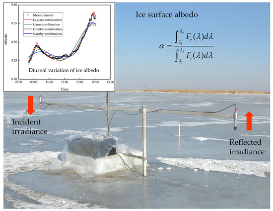
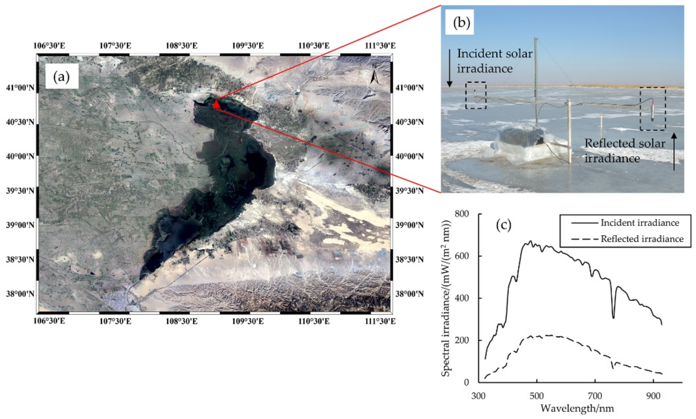
In the present work, a Trios spectral irradiance sensor was used. This sensor can obtain reliable spectral irradiance records each minute, from which the broadband lake-ice albedo can be calculated as the ratio of integrated upwelling to downwelling irradiance [16]. From a physical standpoint, the variation of the surface albedo from sunrise to sunset should be bimodal. However, previous observation technologies used for observing albedo had low sensitivity [17,23] and recorded with a low frequency. Therefore, their results cannot show the detailed bimodal curve. Even considering the small amount of solar flux in the morning and evening, and the impact of scattering [17,18], the albedo curve is still bimodal for solar altitude angles greater than 5°. However, in the period when the solar altitude is greater than 15°, the albedo curve shows a U shape, in which two peaks appear at both ends [17]. For the U-shaped case, it is believed that an exponential relationship exists between the albedo and the solar altitude [13,15]. The U-shaped curve is often separated into two parts to analyze the respective relationships between solar altitude and albedo. The form of exponential function cannot present peaks, and thus overestimates the albedo at times close to sunrise and sunset. Some researchers have replaced the exponential function by cubic functions to describe the bimodal characteristic of the albedo curve [24]. Numerous probability density functions maintain exponential forms that have bilateral symmetrical or asymmetrical peaks, although the exponents are complex in expressions. Therefore, it is desirable to establish a universal expression using these probability density functions that can not only retain the common exponential relationships between albedo and solar altitude, but also describe the bimodal characteristic of albedo curves.

The ice surface albedo is a crucial parameter in the simulation of ice phenology using numerical models. In lake ice models, the ice albedo is often based on parameterizations derived from measurements in high Arctic lakes [25,26]. However, it should be noted that the ice surface albedo may vary between lakes in the high and middle latitudes of the northern hemisphere due to meteorological differences. Robinson et al. (2021) found that regionally specific measurements of the albedo can improve the accuracy of lake ice simulations [27]. Furthermore, the lake ice albedo is affected by the solar zenith angle, and thus varies within a day. In contrast, the currently used parameterizations cannot reflect this property of the lake ice albedo. Therefore, a parameterization that describes the diurnal variation of the ice albedo is necessary. For these reasons, observations on the ice surface albedo were conducted at Wuliangsuhai Lake, and the data was used to describe the diurnal variation of the lake ice albedo. Based on the data, a mathematical expression using the Laplace probability density function was established to model the diurnal cycle in the lake ice albedo. The remainder of this paper is laid out as follows: Section 2 provides details of the observation method and introduces the construction of the statistical model. Section 3 presents the characteristics of the diurnal variation of the lake ice albedo. The simulation of the ice surface albedo is also conducted and evaluated in this section. In Section 4, we further compare our results with other previously reported measurements, and discuss the parameters of mathematical models, and the effects of clouds and atmospheric deposition on the ice surface albedo. Finally, conclusions are drawn in Section 5.

2. Materials and Methods

2.1. Field Observation

Comprehensive surveys of air–ice–water–sediment physics and water ecology were carried out in winter, in conjunction with the National Observation and Research Station of the Wuliangsuhai Wetland Ecosystem in Inner Mongolia. Wuliangsuhai Lake is one of the key wetlands in the semi-arid area in Northwest China, and it provides a critical habitat for migratory water birds in the East Asian–Australasian Flyway and the Central Asian Flyway [28]. It is a river trace lake because of the diversion of the Yellow River [29]. Thus, it has a large area of about 300 km² but a shallow depth of 0.5–1.5 m, with an altitude of 1020 m (Figure 1a). As a result of the shallow and uniform lake depth, the hydrodynamic conditions in this lake are weak. The lake is surrounded by farmland, desert, and saline-alkali land with dense reeds along the shore. The lake freezes every winter from November to the following April, with a typical maximum ice thickness of 60–70 cm. The ice surface is flat with few ridges. Snow occasionally occurs on the ice surface during winter, and sometimes sand and dust is carried onto the ice or snow surface by the wind. The number of sunny days is greater than the number of cloudy days. On sunny days, the sunshine period lasts longer than eight hours, but the maximum solar altitude is only approximately 25–48°. More details on the ice and environmental conditions at Wuliangsuhai Lake during winter can be found in [2,30].

As a part of the survey, field observations on the lake ice albedo were investigated at Wuliangsuhai Lake from 16 January to 11 February in the winter of 2019. Wuliangsuhai Lake has a short thaw period from March to April, and our measurements were taken only during the winter period for safety. With the exception of the first and last days without all-day observations, during the observation period, there were 15 sunny days and 10 cloudy days in total. The observation site was always fixed on an open-ice surface about 1 km from the reeds on the shore, with sporadic snow patches up to 5 mm thick on the surface. Visible gas bubbles were present in the ice, and no snow fall occurred during the investigation period. During the observations, the mean air temperature was −11.0 °C. The coldest daily range of air temperature was from −31.2 to −13.4 °C, and the warmest range was from −10.0 to −1.6 °C.

Two Trios spectral irradiance sensors were fixed at a height of 1.0 m from the ice surface, facing upward and downward (Figure 1b). The sensors recorded incident and reflected spectra irradiance at an interval of 1 minute in the daytime from approximate sunrise to sunset. The spectral range of the irradiance sensor is 320–950 nm, divided into 190 bands of 3.3 nm (±0.3 nm) width, and the accuracy is (±6–10%). Figure 1c shows the typical incident and reflected spectra irradiances measured by the sensors at 12:00 on 22 January Due to the oxygen absorption lines around 760 nm, there was a drop in the spectral irradiance at 750–775 nm. The area within a 20 m radius of the projection point of the downward sensor was covered by ice. Snow patches in other areas did not affect the reflectance spectrum.

The spectral albedo is defined as the ratio of the upwelling irradiance to the downwelling irradiance above the ice cover. Similarly, the broadband albedo is defined as the ratio of the integration of both irradiances within the spectrum range (Equation (1)). Therefore, all data were interpolated first to a 1 nm grid before integration.

$$\alpha =\frac{{\displaystyle {\int }_{{\lambda }_1}^{{\lambda }_2}{F}_{\mathrm{r}}(\lambda )d\lambda }}{{\displaystyle {\int }_{{\lambda }_1}^{{\lambda }_2}{F}_{\mathrm{i}}(\lambda )d\lambda }}$$

(1)

in which α is the broadband albedo from wavelength λ₁ to λ₂; F_r and F_i are reflected and incident spectral irradiances, respectively.

2.2. Simulation for Diurnal Cycle of Ice Albedo on Sunny Days

Two independent influencing factors—the solar altitude and the ice surface characteristics—need to be considered to build a parameterization model of the underlying surface albedo. The two elements are combined in multiplicative or additive forms to affect the albedo [31]. Furthermore, the form of the parameterization should conform to the basic characteristics of the diurnal variation of the albedo.

The diurnal variation of the lake ice albedo on sunny days at Wuliangsuhai Lake is bimodal (see details in Section 3.1). The ice surface albedo at night is neglected, and thus, the ice surface albedo can be regarded as a periodic variation with the period of a day. The shapes of the probability density functions often have peaks. Therefore, it is possible to establish a bimodal parameterization model by linearly combining two probability density functions. Furthermore, with a phase difference on the timeline, the asymmetry peaks of the albedo–time curve are then able to be exhibited [32]. Moreover, considering that various studies may require the ice surface albedo at different time ranges during a day, the newly constructed model has to be able to simulate not only the asymmetrical M-shaped curve of the diurnal variation of the albedo, but also the U-shaped curve between the two peaks when the solar altitude is higher. An additional benefit of applying the combined probability density functions is avoiding the complexity of the previously used piecewise functions.

In this paper, the commonly used probability density functions, Laplace, Gauss, Gumbel, and Cauchy, were selected. The candidate models were then combined as below. The Laplace combination is:

$$f\left(t\right)=\frac{a_1}{2{\sigma }_1}\exp (\frac{-\left|t-{\mu }_1\right|}{{\sigma }_1})+\frac{a_2}{2{\sigma }_2}\exp (\frac{-\left|t-{\mu }_2\right|}{{\sigma }_2})$$

(2)

The Gauss combination is:

$$f\left(t\right)=\frac{a_1}{\sqrt{2\pi }{\sigma }_1}\exp [-\frac{{\left(t-{\mu }_1\right)}^2}{2{\sigma }_1^2}]+\frac{a_2}{\sqrt{2\pi }{\sigma }_2}\exp [\frac{-{\left(t-{\mu }_2\right)}^2}{2{\sigma }_2^2}]$$

(3)

The Gumbel combination is:

$$f\left(t\right)=y_0+\frac{a_1}{{\sigma }_1}\exp [-{\lambda }_1-\exp (-{\lambda }_{{}_1})]+\frac{a_2}{{\sigma }_2}\exp [-{\lambda }_2-\exp (-{\lambda }_2)]$$

(4)

in which, ${\lambda }_1=\frac{t-{\mu }_1}{{\sigma }_1}$, ${\lambda }_2=\frac{t-{\mu }_2}{{\sigma }_2}$.

The Cauchy combination is:

$$f\left(t\right)=\frac{a_1{\sigma }_1}{\pi {\left(t-{\mu }_1\right)}^2+{\sigma }_1^2}+\frac{a_2{\sigma }_2}{\pi {\left(t-{\mu }_2\right)}^2+{\sigma }_2^2}$$

(5)

In the above models, the subscripts 1 and 2 represent the first peak and the second peak, respectively; a is the overall simulation coefficient; μ is the position coefficient taking the time of corresponding peak; t is the time with the unit of day; σ is the actual scale coefficient of corresponding peaks. Considering the minor proportion of solar radiation and the influence of scattering at sunset and sunrise [17,22], the albedo with a solar altitude higher than 5° was selected for subsequent simulation [33]. Therefore, a total of 6 coefficients were required for each model by fitting the albedo on each sunny day. In this manner, the simulation can be completed; however, the coefficients are independent, and the purpose of parameterization is not achieved.

Further analysis showed that the actual scale coefficient can be related to the duration between sunrise and sunset. Therefore, an additional parameter, which is defined here as the scale deformation parameter g, was introduced to the actual scale coefficient, as shown in Equations (6) and (7):

$${\sigma }_1=g_1\left(D-C\right)$$

(6)

$${\sigma }_2=g_2\left(D-C\right)$$

(7)

in which the times of sunrise and sunset (solar altitudes equal to 0° in the morning and afternoon) are set as C and D, respectively. A theoretical formula exists to calculate the times of sunrise and sunset based on the local latitude, longitude, and the Julian calendar [34]. Details can be found in Appendix A.

Moreover, it was found that the scale deformation parameters have parabolic relationships with the time of sunrise (Equations (8) and (9)).

$$g_1=L_1\cdot C^2+M_1\cdot C+N_1$$

(8)

$$g_2=L_2\cdot C^2+M_2\cdot C+N_2$$

(9)

in which L, M, N are the fitting coefficients given in

Table 1. The fitting parameters and determination coefficients (R²) at a significance level of 0.01 of Equations (8) and (9).

Model	L1	M1	N1	R2	L2	M2	N2	R2
Laplace	−93.589	56.939	−8.094	0.998	−93.589	56.939	−8.094	0.998
Gauss	−43.254	26.555	−3.769	0.998	−49.789	30.606	−4.357	0.998
Gumbel	−6.245	3.998	−0.586	0.790	−43.199	26.151	−3.761	0.998
Cauchy	−136.430	82.683	−11.859	0.998	−137.250	82.281	−11.932	0.998

. The determination coefficients are of the same order of magnitude for all models, and the ratios between the fitting parameters are almost the same among the models. In addition, the actual scale parameters of the first and second peaks of the Gumbel combination are significantly different, and those of the two peaks of the Laplace combination are exactly the same.

The position coefficients were also able to be related linearly to the sunrise time, as shown in Equations (10) and (11). The determination coefficients were almost 1.0 at a significance level of 0.01.

$${\mu }_1=0.897\cdot C+0.096$$

(10)

$${\mu }_2=-0.624\cdot C+0.907$$

(11)

The above parameterizations (Equations (6)–(11)) indicate that the coefficients are able to be determined using the geographical location and the Julian calendar, with the exception that the overall simulation coefficients are obtained by assigning the precalculated coefficients (μ₁, μ₂, σ₁, and σ₂) to the simulation models and by performing multivariate regression.

3. Results

3.1. Diurnal Variation of Lake Ice Albedo

An example of the variations of incident and reflected irradiances in the daytime on a clear day (22 January) is shown in Figure 2. Before sunrise (08:03 in Beijing time, UTC + 8), both incident and reflected irradiances were 0. After the sun rose, both irradiances increased and reached the peaks at noon (12:56). Afterwards, the irradiances weakened and dropped to approximately 0 at the end of the observation. It is noteworthy that the peak of the irradiance was much sharper than that of the reflected irradiance. The increasing and declining slopes of the incident irradiance were almost constant in the morning and afternoon, and were higher than those of the reflected irradiance. The ratio of the reflected to incident irradiances, i.e., the ice surface albedo, showed an M shape from sunrise to sunset.

Figure 3 shows the typical curves of diurnal changes in the ice surface albedo under five different weather conditions. It was sunny on 22 January, but the ice surface albedo was not always the highest at any time compared with the other curves. The curve was smooth and had less noise. The calculated sunrise, solar noon, and sunset times in Beijing time are given in

Table 2. The sunrise, solar noon, and sunset times of the days in Figure 3 (Beijing Time).

Date	Sunrise	Solar Noon	Sunset
17 January	08:06	12:55	17:44
18 January	08:06	12:55	17:45
22 January	08:03	12:56	17:50
28 January	07:59	12:58	17:57
30 January	07:57	12:58	17:59

. The albedo–time curve had two peaks occurring in the morning and afternoon. The first occurred approximately 1.5 h after sunrise, with a solar altitude of 13.1–14.4°, whereas the second occurred roughly 0.8 h before sunset, with a solar altitude of 4.8–8.9°. The two peak values were quite different, exhibiting an obvious asymmetric characteristic. The trough on the curve occurred approximately in the middle of the day, with a solar altitude angle ranging from 28.7 to 32.5°. Taking solar noon in Beijing time (12:00) as the axis of symmetry, the curve is also asymmetric, with a different length from the peak to the symmetry axis due to the time difference between local time and Beijing time. Therefore, the albedo curves have an M shape from sunrise to sunset.

The diurnal variation of albedo showed a high correlation with cloud cover. It was partly cloudy on 18 January, and the ice surface albedo was slightly less than that on a sunny day. The albedo curve was also M shaped but with a higher degree of noise, indicating the influence of cloud cover and location. In addition, the first peak appeared 0.5 h later than on the sunny day, whereas the second peak appeared 2.0 h earlier than on the sunny day. While as it was overcast in morning (28 January), the first peak was not apparent on the albedo–time curve. In contrast, a partly cloudy afternoon resulted in a lower second peak (17 January). The diurnal variation of the ice surface albedo on an overcast day still maintained the two symmetrical peaks (28 January). The first peak appeared about 0.5 h later than on a sunny day, whereas the second peak was 1.5 h earlier than on a sunny day. However, the peak values were significantly less than on a sunny day. The albedo was almost constant between the two peaks.

Because the literature-reported ice surface albedos are generally measured around local solar noon, both the average albedos (Equation (12)) and weighted averages by incident intensity (Equation (13)) were determined from sunrise to sunset and during 11:00–14:00.

Table 3. The average albedos and weighted average albedos under different weather conditions.

Date	Average Albedo		Weighted Average Albedo
	Sunrise–Sunset	11:00–14:00	Sunrise–Sunset	11:00–14:00
17 January	0.302	0.289	0.303	0.289
18 January	0.286	0.288	0.294	0.289
22 January	0.324	0.285	0.320	0.285
28 January	0.285	0.267	0.283	0.268
30 January	0.254	0.253	0.256	0.253

provides the calculation results using the data in Figure 3. On the sunny day, 22 January, the mean albedo during the period from sunrise to sunset was 0.324, and the weighted average was 0.320. The two types of averages were both 0.285 during 11:00–14:00. This indicates that calculating the average albedo containing the two peaks yields a higher result. Bolsenga (1969) reported that the albedo in the 300–3000 nm band on a sunny day was 0.10 for pure lake ice and 0.22 for bubble-containing lake ice [11]. Our results are greater than the previously reported values, probably because there are much more visible bubbles in the lake ice at Wuliangsuhai Lake, leading to an increase in the albedo. Furthermore, it was found that the mean albedos from both periods were approximately equal to 0.25 on the overcast day (30 January), which is lower than those on the sunny day.

$$\overline{\alpha }=\frac{1}{n}{\displaystyle \sum _{j=1}^{j=n}{\alpha }_j}$$

(12)

$${\overline{\alpha }}_{\mathrm{w}}=\frac{{\displaystyle \sum _{j=1}^{j=n}{\displaystyle {\int }_{{\lambda }_1}^{{\lambda }_2}{F}_i(\lambda )}}\times {\alpha }_j}{{\displaystyle \sum _{j=1}^{j=n}{\displaystyle {\int }_{{\lambda }_1}^{{\lambda }_2}{F}_{\mathrm{i}}{(\lambda )}_j}}},$$

(13)

in which $\overline{\alpha }$ is the mean albedo; ${\overline{\alpha }}_{\mathrm{w}}$ is the weighted albedo; n is the amount of the measured albedo during a day.

3.2. Simulating the Diurnal Cycle of Lake Ice Albedo on a Sunny Day

The four combined probability density function models were applied to fit the observed albedo with a solar altitude of ≥5° on a sunny day (29 January). As shown in Figure 4a, for the Cauchy combination model, the two peaks and the simulation at low solar altitude angles were lower than the actual measurements. The simulated albedo values around solar noon with higher solar altitudes were higher than the field measurements. Additionally, the varying slopes around the simulated peaks were lower, resulting in a delayed first simulated peak and an advanced simulated second peak, compared to the actual measurements. The albedo peaks simulated using the Gauss combination were slightly higher than the simulation by Cauchy combination, but nonetheless lower than the actual peaks. Compared with the actual peaks, the first and second simulated peaks also occurred later and earlier, respectively. The Gauss combination model underestimated the trough of the albedo curve, and only fit the data well in the declining and ascending parts between the two peaks. Therefore, the Gauss combination is suitable for simulating the U-shaped curve of the diurnal albedo with a solar altitude angle higher than 15°, but is not suitable for the M-shaped curve of the diurnal albedo with a solar altitude angle higher than 5°.

The Gumbel combination was a good fit for the first peak in terms of value and position, but a relatively poor fit for the second peak. The simulated second peak was lower and earlier than the actual measurement. In addition, the trough simulated by the Gumbel combination was flatter around solar noon. The Laplace combination fitted the observed albedo curve best. The simulated peaks had a sharp shape, resembling the measured peaks only with slight overestimates, as there is a sharp peak in the curve of Laplace function itself. The simulated positions of peaks also corresponded accurately. The simulated curve between the two peaks was also close to the actual observations.

The comparisons between the albedo simulated by the four models and the on-site measured albedo are given in Figure 4b. There was a total of 518 on-site measured albedos ranging from 0.25 to 0.38 on 29 January With the exception of the Laplace model, the simulated albedos using the models were lower than the observed values at the peaks. The correlation coefficient, root mean square error, mean absolute error, and mean error ± standard deviation are shown in

Table 4. The correlation coefficients r, root mean square errors (RMSE), mean absolute errors (MAE), and mean errors ± standard deviations (Mean ± Std.) (simulated minus measured albedo) of four models for albedo with a solar altitude ≥ 5° on 29 January.

Model	r	RMSE	MAE	Mean ± Std.
Laplace	0.990	0.0049	0.0038	−0.0004 ± 0.0049
Gauss	0.952	0.0108	0.0089	0.0004 ± 0.0108
Gumbel	0.979	0.0070	0.0050	−0.0001 ± 0.0070
Cauchy	0.971	0.0084	0.0079	−0.0003 ± 0.0084

. Of the four models, the Laplace combination model performs better in terms of all four of the indexes.

By making the comparison to all 6231 albedo values with a solar altitude ≥ 5° on 12 sunny days during the entire investigation period, we further evaluated the simulation results of the four models with the observation results (Figure 5).

Table 5. The correlation coefficients and errors (simulated minus measured albedo) of the four models of albedo within the time range of the solar altitude angle of ≥5° during 12 sunny days.

Model	r	RMSE	MAE	Mean ± Std.
Laplace	0.972	0.0106	0.0080	−0.0001 ± 0.0106
Gauss	0.931	0.0164	0.0124	−0.0003 ± 0.0164
Gumbel	0.970	0.0112	0.0075	−0.0023 ± 0.0110
Cauchy	0.940	0.0154	0.0112	−0.0009 ± 0.0154

shows the correlation and error analysis results, which further confirms that the Laplace combination is the optimal model.

Figure 6 plots the simulated albedo using the Laplace model for the diurnal variations on the 12 sunny days against the observed data. The correlation coefficients and errors between the simulated and measured data of each day were calculated (

Table 6. Correlation coefficients, errors (simulated minus measured albedo), and overall simulation coefficients a₁ and a₂ derived for the Laplace combination.

Date	r	RMSE	MAE	Mean ± Std.	a1	a2
16 January	0.976	0.0115	0.0094	0.0004 ± 0.0111	0.1014	0.1458
20 January	0.984	0.0089	0.0068	0.0006 ± 0.0090	0.0938	0.1449
22 January	0.959	0.0155	0.0098	0.0008 ± 0.0154	0.0936	0.1472
23 January	0.985	0.0074	0.006	0.0004 ± 0.0074	0.0949	0.1377
25 January	0.967	0.0103	0.0083	0.0001 ± 0.0103	0.0921	0.1338
29 January	0.990	0.0049	0.0038	−0.0004 ± 0.0049	0.0903	0.1315
31 January	0.926	0.0093	0.0071	−0.0011 ± 0.0094	0.0961	0.1232
1 February	0.971	0.0084	0.006	0.0001 ± 0.0085	0.0942	0.1342
3 February	0.984	0.0059	0.0048	0.0005 ± 0.0059	0.0946	0.1329
4 February	0.916	0.0075	0.0052	0.0002 ± 0.0076	0.0779	0.1816
8 February	0.919	0.0141	0.0117	0.0007 ± 0.0140	0.1088	0.1261
11 February	0.942	0.0101	0.0074	0.0000 ± 0.0102	0.0956	0.1373

). The correlation coefficients are all at a high level, and the maximum root mean square errors of the 12 days are less than 0.016. The overall simulation coefficients of the model derived from the albedo for each day are also listed in Table 6.

4. Discussion

4.1. Comparisons with the Diurnal Cycle of Ice Albedo in Melt Period

Wuliangsuhai Lake has a short thaw period from March to April. Field work on melting ice in mid-latitude lakes is dangerous, and our measurements were only undertaken during the winter period. Therefore, the applicability of our parameterization for the ice albedo in the spring thaw period needs to be validated in future work. Few studies have reported the diurnal cycles of snow/ice albedos in the melt season. Pirazzini et al. (2006) measured the sea ice surface albedo in the Baltic Sea during the spring snowmelt period, and found that, during clear days, the ice albedo showed a relatively strong decline in the morning and then maintained a slight increase in the afternoon [20]. The highest values of albedo occurred during the early morning, and were attributed to the frozen surface layer of snow covered by highly scattering small crystals, which is formed due to frost or rime formation during the previous night. Similar declining trends in the surface albedo over melting ice and snow during the daytime were also reported in Jakkila (2009) [21] and Zdorovennova et al. (2018) [22] in boreal lakes. The lack of an increase in surface albedo found in [21,22] was probably dependent on the thickness, grain, and metamorphism of the snow cover. In contrast, in our measurements, only sporadic snow patches existed with a thickness of up to 5 mm. The decrease in the lake ice albedo during the morning, and the increase during the afternoon, were associated with the solar altitude angle, and the asymmetrical shape was mainly attributed to the effects of cloud cover and light-absorbing impurities on the surface.

Recently, we developed a platform that is equipped with various sensors for observing the ice properties throughout the whole ice period. Using this platform, we can measure and compare the lake ice albedo in different periods, making it possible to parameterize the diurnal variation of lake ice albedo during different ice periods. Furthermore, because the time length of the ice period between mid- and high-latitudes is different, the representative ice properties, such as ice thickness or ice temperature, may be used as indexes of the ice period to be included into the parameterization of the diurnal variation of the ice albedo.

4.2. On the Statistical Models

Probability density functions are commonly used to undertake statistical analysis and describe the trends of periodic hydro-meteorological events, and to predict the frequency and time of their occurrence. The greatest advantage of probability density functions is the ability to define event lengths and peak heights, which also reduces the uncertainty in the analysis of the long-term flood distribution [35]. In other connections in surface water and groundwater, ecology, and agriculture, these functions have been applied to the assessment of the impact of climate change on hydrology and the agro-ecological environment [36].

There are also other mathematical models with peaks and random parameters [37]. For local hydrological processes with a random nature, probability density functions without shape parameters produce poor fits. Therefore, models with two shape parameters are needed. The diurnal variations of albedo are regular depending on the time and the geographical conditions. The coefficients of the statistical model developed in this paper are linked to the regional sunrise and sunset times, and thus, the model is meaningful in the context of physics. Therefore, it is not necessary to apply a three-parameter or four-parameter distribution model with shape parameters to satisfy the temporal and spatial variations of the ice surface [38].

From the perspective of developing a parameterization scheme, the Laplace combination with the same actual scale coefficients (Table 1) can simplify the calculation steps. Table 6 shows the overall simulation coefficients a₁ and a₂ of the Laplace model. The overall simulation coefficients determine the level of albedo. The overall simulation coefficients vary, showing that there are other secondary factors, in addition to solar altitude angle and cloud cover, influencing the diurnal changes in the lake ice surface albedo. Theoretically, meteorological factors (e.g., air temperature), ice physical properties (e.g., ice thickness and ice surface roughness), and dust and other dirt, are included in the overall simulation coefficients. The coefficient a₁ is in the range of 0.078–0.109, with an average of 0.094 and a standard deviation of 0.007. The coefficient a₂ is in the range of 0.123–0.182, with an average of 0.140 and a standard deviation of 0.015.

The mean values of a₁ and a₂, to which three times the standard deviation are subtracted or added, are close to the corresponding minimum and maximum, respectively. To investigate the effects of secondary factors, we then used (1) the average and (2) the average ±3 times the standard deviation as inputs to the Laplace model for each sunny day. The differences between the simulated albedos in case (1) and the observed values were less than 5% on each sunny day, whereas those of case (2) were approximately 16%. The absolute error from applying the average overall simulation coefficients was approximately 1%.

4.3. Effect of Clouds on Ice Surface Albedo and Solar Radiation

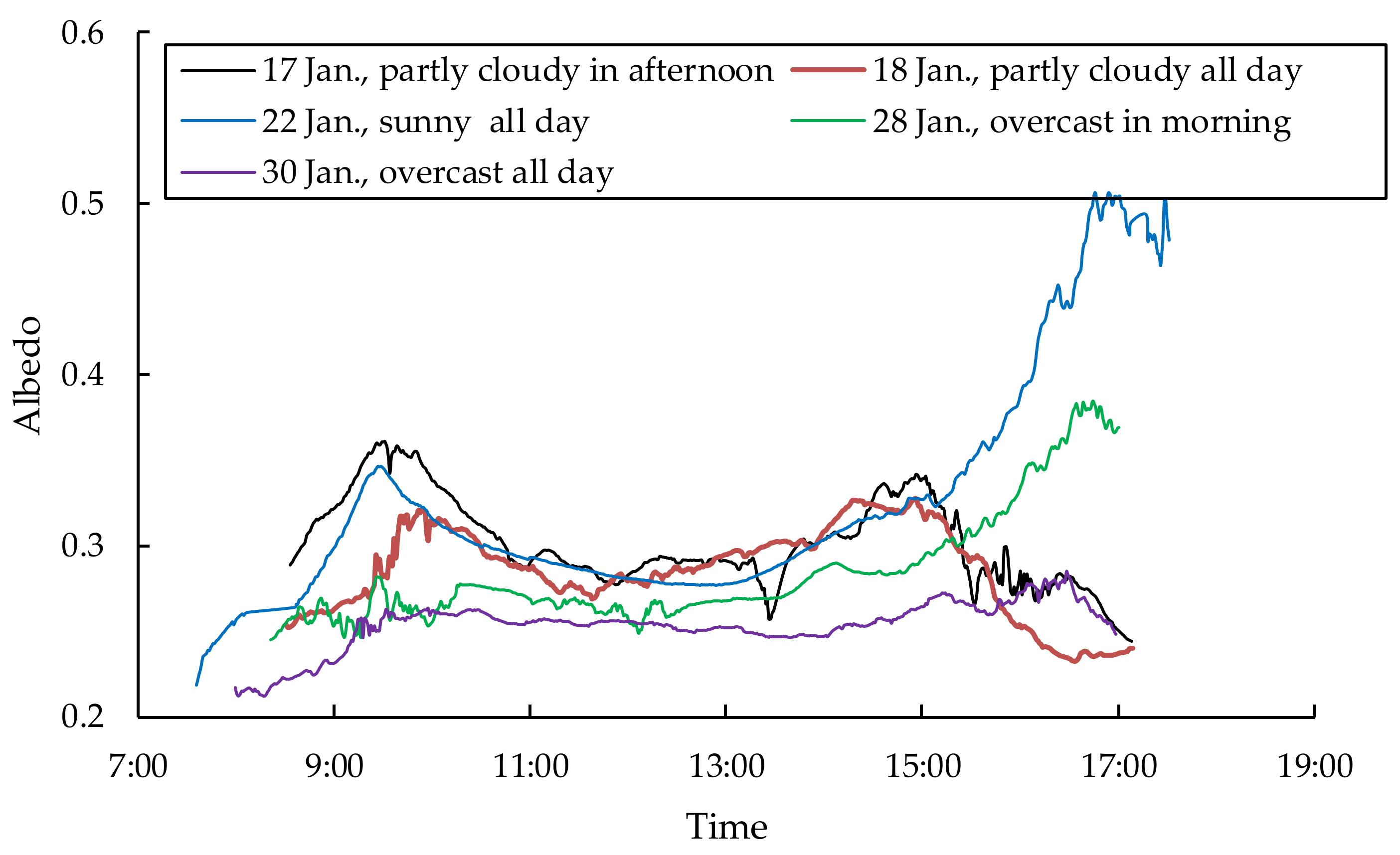
The differences in the albedo during the five different types of weather shown in Figure 3 were mainly due to the influence of cloud cover. The solar radiation is affected by the cloud cover [39]. At any solar altitude angle, the greater the cloud cover, the lower the solar radiation intensity that reaches the ice surface. It was also found that the influence of the cloud cover on the albedo is not only reflected in the values of the peak albedo, but also in the timing of the peak. In general, the first peak appears later in the morning and the second peak appears earlier in the afternoon, on a cloudy day. However, the albedo data collected on the ice surface of Wuliangsuhai Lake under cloudy conditions are insufficient. Particularly lacking are quantitative data for the cloud cover due to the commonly used method of recording in tenths. The classifications generally used to describe the weather, such as sunny, cloudless, partly cloudy, and overcast, are not suitable for a quantitative analysis of the albedo. Therefore, it is not possible to develop a statistical expression of cloud cover using the Laplace model parameters. Previous studies have also only carried out a quantitative analysis of albedo on sunny and overcast days. An increased accumulation of field measurements on cloud cover using a quantitative method will be necessary in the future.

Although Wuliangsuhai Lake is located in the mid-latitudes of the northern hemisphere, there are several days when it is cloudy in winter. The clouds reduce the solar radiation. There are also many ice-covered lakes on the Tibet Plateau, where the solar radiation is more intense. Due to the intense solar radiation, the under-ice water environment and ecosystem, in addition to the air–ice–water mass exchange, are likely different to those of Wuliangsuhai Lake, further influencing the local climate. In contrast, most of the Earth’s ice is located in the polar regions at high latitudes, where it is night or cloudy with low visibility in winters. The low solar radiation in the polar regions is the main source of the difference compared with the melting process of snow and ice in China.

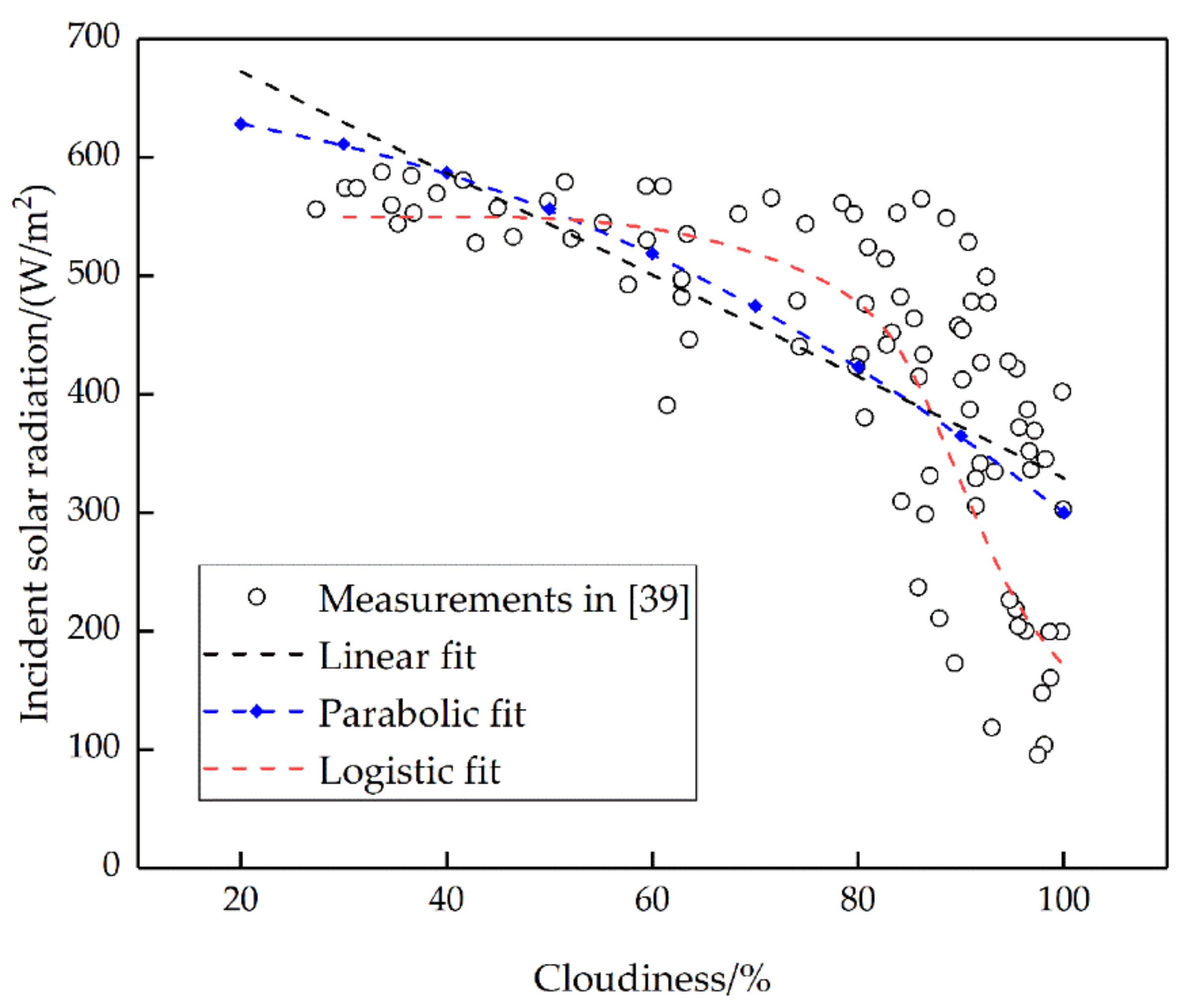
It has been reported that solar radiation decreases linearly with increased cloudiness in the semi-arid region in Western China (Figure 7) [39]. The previously reported relationship is given by Equation (14). However, the trend in the variation of incident solar radiation with respect to cloudiness shown in Figure 7 is actually non-linear, and the linear fit is not appropriate.

$${\varphi }_{\mathrm{cl}}=-4.29C_{\mathrm{l}}+758.41$$

(14)

in which ϕ_cl is the solar radiation at a cloudiness C_l, expressed as a percentage.

In the river ice models, the influence of cloud cover on solar radiation has been evaluated using a parabolic equation in a form of Equation (15) [40]. In the formula, C_l is expressed in tenths, and the solar radiation ϕ₀ can be calculated theoretically once the geographical locations and measurement times are known (see details in Appendix B). However, no detailed information was reported in [39]. Therefore, we conducted a regression analysis using the data exhibited in Figure 7 on the basis of the form of Equation (15), and the refitted expression is given in Equation (16). However, the comparison in Figure 7 shows the parabolic relationship is unable to reflect the variation characteristic of solar radiation with cloudiness.

$${\varphi }_{\mathrm{cl}}={\varphi }_0(1-0.0065C_{\mathrm{l}}{}^2)$$

(15)

in which ϕ₀ is the solar radiation at C_l = 0, and C_l is divided into tenths ranging from 0 to 10.

$${\varphi }_{\mathrm{cl}}=642.05\times [1-0.005{(C_{\mathrm{l}}/10)}^2]$$

(16)

in which C_l is expressed as a percentage.

The trend in the variation of solar radiation with cloudiness shows that, at a cloudiness below 50%, the solar radiation decreases slightly with increased cloudiness, with a value of approximate 550 W/m². However, as cloudiness increases, the incident radiation declines significantly, and reaches 170 W/m² at a cloudiness of 100%. Finally, a logistic model was used to describe this trend, as shown in Equation (17). The determination coefficient was 0.612 at a significance level of 0.01. Compared with linear and parabolic models, the logistic model has a good fit with the nearly stable and rapidly descending parts in the relationship of the solar radiation with cloudiness, and corresponds well with the solar radiation under a clear sky and an overcast state, respectively.

$${\varphi }_{\mathrm{cl}}=\frac{425}{1+2.5\exp (-18.8+0.2C_{\mathrm{l}})}+125$$

(17)

For Wuliangsuhai Lake, the observed solar irradiance was 770 W/m² on the sunny day and 160 W/m² on the overcast day in winter. As previously mentioned, quantitative measurements of the cloud cover on cloudy days are lacking, making it impossible to determine the relationship between solar radiation and cloudiness. We believe that, with an increased accumulation of field measurements of the cloud cover, the logistic model may also be appropriate for the solar radiation–cloudiness relationship in Wuliangsuhai Lake.

4.4. Effect of Atmospheric Deposition on Ice Surface Albedo

In addition to air temperature, precipitation, and cloud cover, light-absorbing dust, black carbon, and organic carbon significantly reduce the albedo. They also play a role in snow and ice melt [41]. The impact of black carbon and organic carbon on albedo is better known than that of sand dust. In the arid and semi-arid areas in China, where desertification predominates, large areas are without snow in winter, and wind may bring sand and dust from the nearby deserts onto the ice, making the surface tawny. Dust particles increase absorption of solar radiation, which melts snow and ice. Particularly during spring, solar radiation at noon provides more heat to the snow/ice surface than that released from snow/ice surface to the atmosphere. The snow/ice surface partially melts, and the melt water flows slowly to the low-lying places, while the sand and dust remains. Due to these processes, the light-absorbing impurities exist not only on the snow and ice surface, but can also be found below the surface. The increased impurity content on and in the snow and ice enhance the snow and ice melt. Because the quantity of sand dust in Northwest China is much greater than that of black carbon and organic carbon, the effect of sand dust is significantly greater than that of organic dust. Furthermore, the impact of the dust on the ice albedo may be heightened near sunset in the melt season because of the continuous melt during the day. However, this impact is not clear during the freezing period. To date, only preliminary conclusions have been reached about the low albedo of sand and dust on the surfaces of glacier ice [13,42] sea ice [43], and lake ice [44]. In particular, studies are lacking on the effect of the temporal variation in light-absorbing impurities on the ice/snow albedo at such short time scales. Therefore, thorough quantitative analysis of the physical process of the impact of sand dust, black carbon, and organic carbon on the albedo is required to enable understanding of the high melting rate of ice in Northwest China.

A Snow, Ice, and Aerosol Radiation (SNICAR) model was developed to study the effect of impurities in snow/ice on the surface albedo [45]. This model can determine the contribution of the size of black carbon particles caused by the atmosphere or automobile exhaust on snow cover, and the distribution of black carbon in snow cover per weight unit in the reduction of the albedo. The SNICAR model can also be used to simulate some tawny substances [46]. However, the basic theory of the model is based on the effect of the particle size of a single component material. Due to the efforts of other researchers, the studies have been extended to simulate not only the influence of the material content, but also the color and content of fuel oil in snow [47], in addition to particles of general atmospheric substances falling on the surface of the snow and ice [48].

In terms of material composition, compared with dust discharged from atmospheric fuel oil, sand dust in Western China has a larger particle size, a higher content, and a tawnier color. In addition, the mixed material composition of dust also contributes to the complexity of the influence on the albedo, and thus, the quantitative description of the influence requires further improvement. The closest research result is the study of the effect of glacial sediments on the albedo of glacial ice. Although this research is somewhat shallower than the research into the influence of atmospheric dust on the surface of the snow/ice on the albedo, it nonetheless provides directions for future efforts. In future, we will rely on a large number of observations of sand and dust on the ice surface and inside the ice [49], in addition to the ice surface albedo. These data will be combined with existing results on the glacier [50] and the model of snow/black carbon/organic carbon (the SNICAR model) to develop a comprehensive understanding of the influences, including cloud cover, dust, and the physical properties of snow/ice [51].

5. Conclusions

Field observations on the ice surface albedo were investigated at Wuliangsuhai Lake, a typical frozen lake of semi-arid cold regions, during the winter of 2019. During the observation period, there were 15 sunny days and 10 cloudy days. The characteristics of the curves showing the variation of the ice surface albedo with time under different weather conditions were analyzed. Furthermore, a total of four commonly used density distribution functions—Laplace, Gauss, Gumbel, and Cauchy—were linearly combined to simulate the diurnal variation of the ice albedo curve on a sunny day.

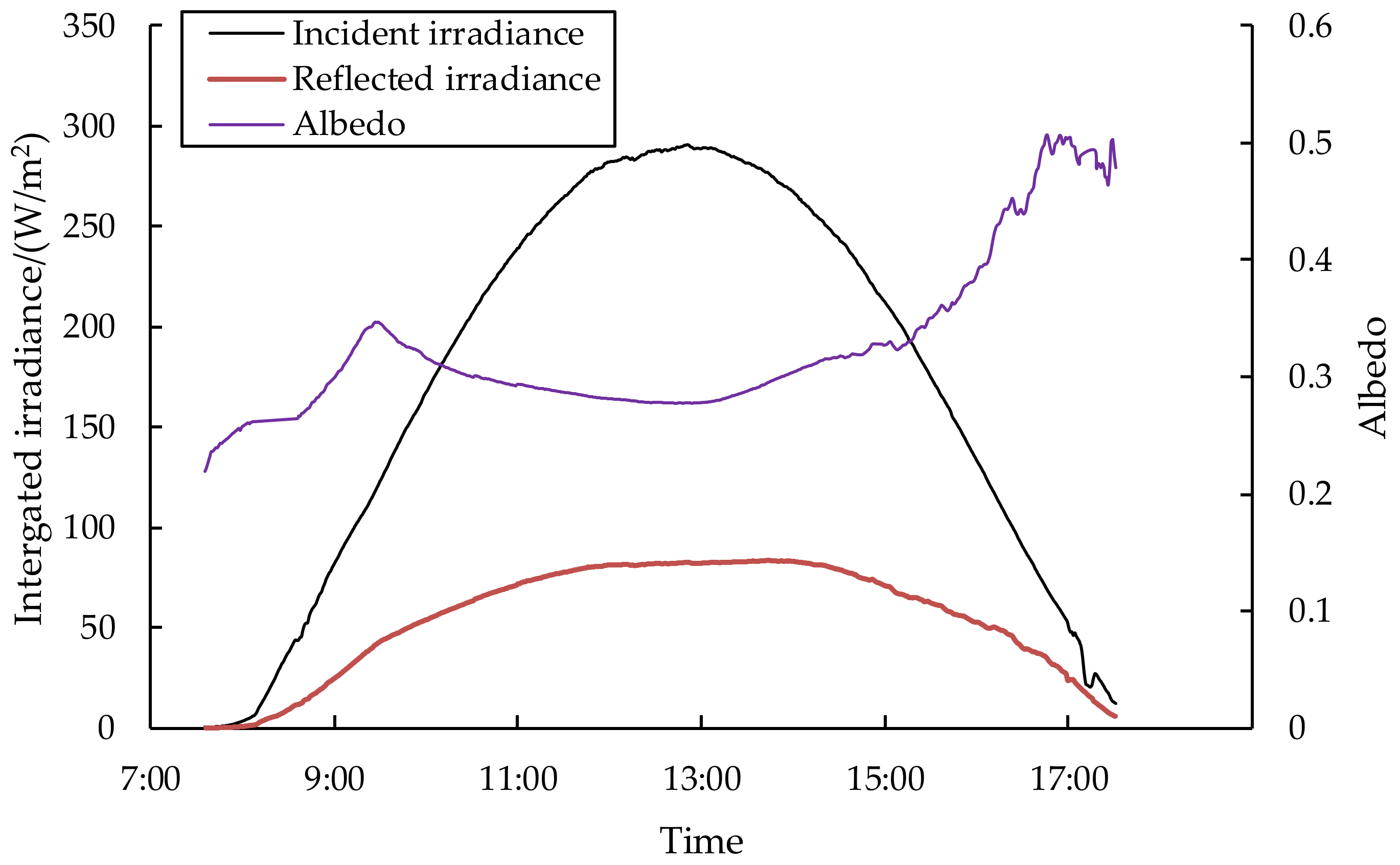
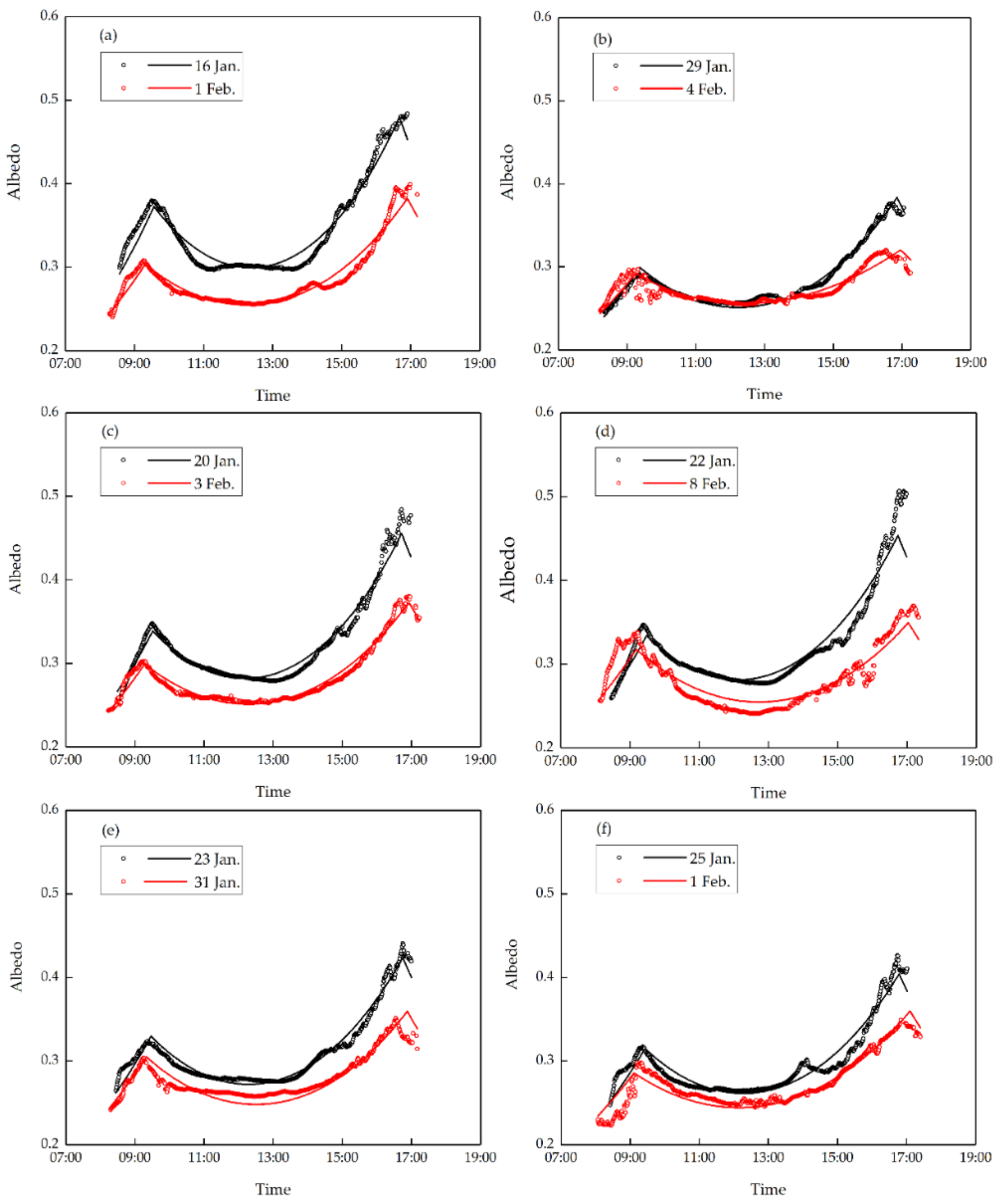
Diurnal variations of the ice surface albedo with time at Wuliangsuhai Lake exhibited two peaks, occurring after sunrise and before sunset. The two peaks were not equal and appeared to be asymmetrical. The diurnal change in the albedo on days with few clouds retained the characteristic of the double peaks, but with additional noise in the curve. The first peak occurred later in partially cloudy days than in sunny days, whereas the second peak appeared earlier than in sunny days. The albedo in cloudy days was low.

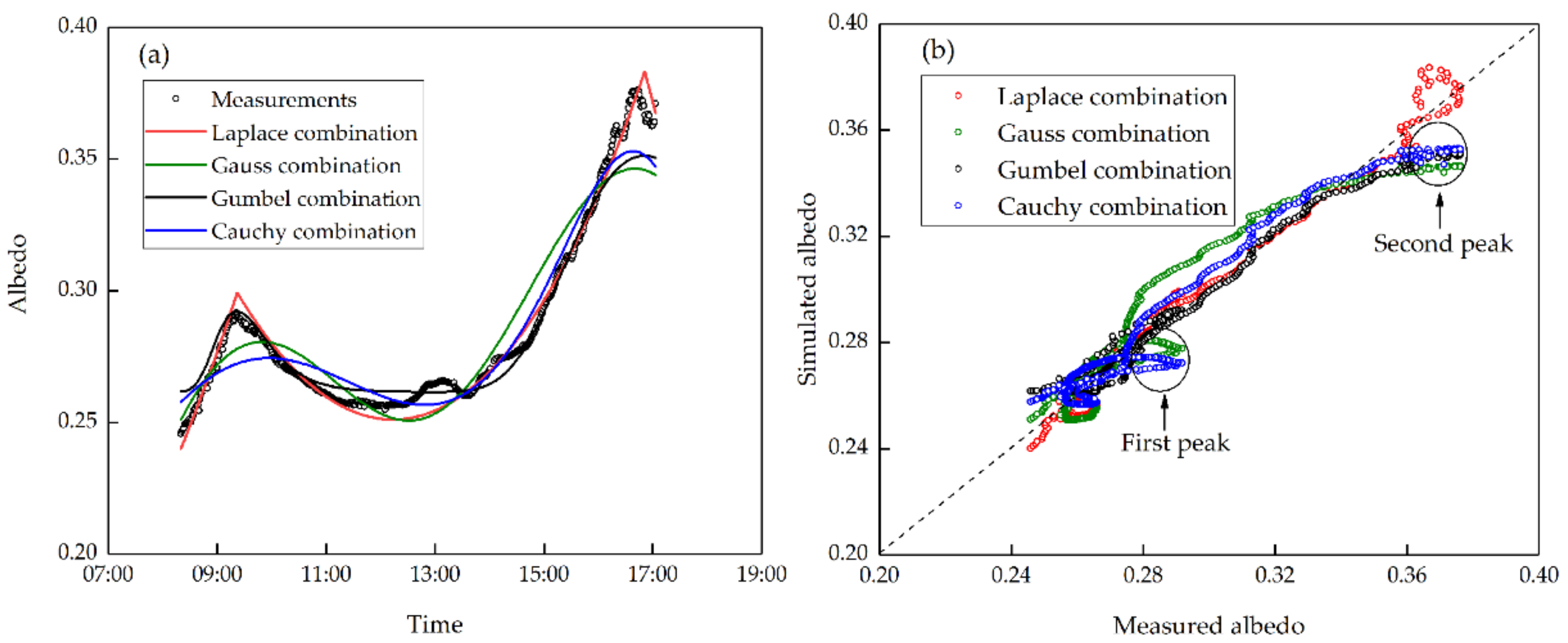
All of the four combined statistical models can simulate the diurnal albedo variation curve with bimodal characteristics and a U shape between the two peaks. The peak coefficients and actual scale coefficients in the models were correlated with sunrise and sunset times, which can be determined using the local latitude, longitude, and the Julian calendar. Comparisons between the simulated and measured albedos using the data with solar altitude angles of ≥5° indicate that the Laplace model performed better than the other models. The Laplace model performed best in depicting the albedo curve characteristics, particularly the peak shape and position, and in error analysis.

The simulation using the measured albedo on each sunny day yielded a set of overall simulation coefficients. Taking the mean overall simulation coefficients as the final inputs, the difference between the simulated and measured albedo on each sunny day was less than 5%. Therefore, the Laplace model using the mean overall simulation coefficients can be treated as the parameterization of the diurnal cycle of the lake ice surface albedo in semi-arid cold regions. However, from the perspective of physical mechanisms, several factors affecting the ice albedo are included in the overall simulation coefficient, such as the change in cloudiness, air temperature, snow, dust, and moisture on the ice surface. More quantitative studies will be required to determine the individual contributions of these factors to improve the understanding of the lake ice albedo mechanism. In addition, due to the expansion of the reed area around Wuliangsuhai Lake in recent years [29], additional effort is also needed to understand the surface albedo of the ice–reed mixture, and thus help to precisely determine the ice edge using optical remote techniques.

References

1. Surdu, C.M.; Duguay, C.R.; Pour, H.K.; Brown, L.C. Ice freeze-up and break-up detection of shallow lakes in Northern Alaska with spaceborne SAR. Remote Sens. 2015, 7, 6133–6159. [Google Scholar] [CrossRef] [Green Version]
2. Song, S.; Li, C.; Shi, X.; Zhao, S.; Tian, W.; Li, Z.; Bai, Y.; Cao, X.; Wang, Q.; Huotari, J.; et al. Under-ice metabolism in a shallow lake in a cold and arid climate. Freshw. Biol. 2019, 64, 1710–1720. [Google Scholar] [CrossRef]
3. Mironov, D.; Terzhevik, A.; Kirillin, G.; Jonas, T.; Malm, J.; Farmer, D. Radiatively driven convection in ice-covered lakes: Observations, scaling, and a mixed layer model. J. Geophys. Res. Ocean. 2002, 107, 3032. [Google Scholar] [CrossRef] [Green Version]
4. Terzhevik, A.; Golosov, S.; Palshin, N.; Mitrokhov, A.; Zdorovennov, R.; Zdorovennova, G.; Kirillin, G.; Shipunova, E.; Zverev, I. Some features of the thermal and dissolved oxygen structure in boreal, shallow ice-covered Lake Vendyurskoe, Russia. Aquat. Ecol. 2009, 43, 617–627. [Google Scholar] [CrossRef]
5. Yang, F.; Li, C.; Leppäranta, M.; Shi, X.; Zhao, S.; Zhang, C. Notable increases in nutrient concentrations in a shallow lake during seasonal ice growth. Water Sci. Technol. 2016, 74, 2773–2783. [Google Scholar] [CrossRef] [Green Version]
6. Sun, C.; Li, C.; Liu, J.; Shi, X.; Zhao, S.; Wu, Y.; Tian, W. First-principles study on the migration of heavy metal ions in ice-water medium from Ulansuhai Lake. Water 2018, 10, 1149. [Google Scholar] [CrossRef] [Green Version]
7. Liu, Y.; Li, C.; Anderson, B.; Zhang, S.; Shi, X.; Zhao, S. A modified QWASI model for fate and transport modeling of mercury between the water-ice-sediment in Lake Ulansuhai. Chemosphere 2017, 176, 117–124. [Google Scholar] [CrossRef]
8. Wei, Y.; Zhang, M.; Cui, L.; Pan, X.; Liu, W.; Li, W.; Lei, Y. Winter decomposition of emergent macrophytes affects water quality under ice in a temperate shallow lake. Water 2020, 12, 2640. [Google Scholar] [CrossRef]
9. Petrov, M.P.; Sutyrin, G.G. Diurnal cycle of convection in an ice-covered lake. Meteorol. Gidrolog. 1984, 1, 91–98. [Google Scholar]
10. Pushistov, P.Y.; Ievlev, K.V. Numerical eddy-resolving model of nonstationary penetrative convection in spring solar heating of ice-covered lakes. Bull. Inst. Comput. Math. Math. Geophys. 2000, 5, 55–63. [Google Scholar]
11. Bolsenga, S.J. Total albedo of Great Lakes ice. Water Resour. Res. 1969, 5, 1132–1133. [Google Scholar] [CrossRef]
12. Dahlback, A.; Gelsor, N.; Stamnes, J.; Gjessing, Y. UV measurements in the 3000–5000 m altitude region in Tibet. J. Geophys. Res. 2007, 112, D09308. [Google Scholar] [CrossRef]
13. Jiang, X.; Wang, N.; Pu, J.; He, J.; Chen, L. Variations of albedo and spectral reflectance on Qiyi Glacier in Qilian Mountains during the ablation season. Sci. Cold Arid Reg. 2009, 1, 59–70. [Google Scholar]
14. Wang, X.; Zender, C.S. Arctic and Antarctic diurnal and seasonal variations of snow albedo from multiyear Baseline Surface Radiation Network measurements. J. Geophys. Res. Earth Surf. 2011, 116, F03008. [Google Scholar] [CrossRef] [Green Version]
15. Yao, T.; Zhang, Q. Study on land-surface albedo over different types of underlying surfaces in North China. Acta Phys. Sin. 2014, 63, 089201. (In Chinese) [Google Scholar] [CrossRef]
16. Norsang, G.; Jin, Y.; Tsoja, W.; Zhou, Y.; Sunam, B.; Denggua, T. Ground-based measurements of global solar radiation and UV radition in Tibet. Spectrosc. Spectr. Anal. 2019, 39, 1683–1688. (In Chinese) [Google Scholar] [CrossRef]
17. Xiao, Y.; Zhao, L.; Li, R.; Yao, J.; Sun, L.; Qiao, Y.; Jiao, K. The characteristics of surface albedo in permafrost regions of northern Tibetan plateau. J. Glaciol. Geocryol. 2010, 32, 480–488. (In Chinese) [Google Scholar]
18. Sun, J.; Hu, Z.; Xun, X.; Peng, W.; Lv, B.; Xu, L. Albedo characteristics in different underlying surfaces in mid- and upper-reaches of HEIFE and its impact factor analysis. Plateau Meteorol. 2011, 30, 607–613. (In Chinese) [Google Scholar]
19. Pirazzini, R. Challenges in snow and ice albedo parameterizations. Geophysica 2009, 45, 41–62. [Google Scholar]
20. Pirazzini, R.; Vihma, T.; Granskog, M.A.; Cheng, B. Surface albedo measurements over sea ice in the Baltic Sea during the spring snowmelt period. Ann. Glaciol. 2006, 44, 7–14. [Google Scholar] [CrossRef] [Green Version]
21. Jakkila, J.; Leppäranta, M.; Kawamura, T.; Shirasawa, K.; Salonen, K. Radiation transfer and heat budget during the ice season in Lake Pääjärvi, Finland. Aquat. Ecol. 2009, 43, 681–692. [Google Scholar] [CrossRef]
22. Zdorovennova, G.; Palshin, N.; Efremova, T.; Zdorovennov, R.; Gavrilenko, G.; Volkov, S.; Bogdanov, S.; Terzhevik, A. Albedo of a small ice-covered boreal lake: Daily, meso-scale and interannual variability on the background of regional climate. Geosciences 2018, 8, 206. [Google Scholar] [CrossRef] [Green Version]
23. Bolsenga, S.J.; Greene, G.M. Techniques to measure the spectral reflectance of ice. Proc. SPIE 1984, 489, 384–391. [Google Scholar] [CrossRef]
24. Minnis, P.; Mayor, S.; Smith, W.L.; Young, D. Asymmetry in the diurnal variation of surface albedo. IEEE Trans. Geosci. Remote Sens. 1997, 35, 879–891. [Google Scholar] [CrossRef] [Green Version]
25. Duguay, C.R.; Flato, G.M.; Jeffries, M.O.; Menard, P.; Morris, K.; Rouse, W.R. Ice-cover variability on shallow lakes at high latitudes: Model simulations and observations. Hydrol. Process. 2003, 17, 3465–3483. [Google Scholar] [CrossRef]
26. Yang, Y.; Leppäranta, M.; Cheng, B.; Li, Z. Numerical modelling of snow and ice thicknesses in Lake Vanajavesi, Finland. Tellus Ser. A Dyn. Meteorol. Oceanol. 2012, 64, 17202. [Google Scholar] [CrossRef] [Green Version]
27. Robinson, A.L.; Ariano, S.S.; Brown, L.C. The Influence of snow and ice albedo towards improved lake ice simulations. Hydrology 2021, 8, 11. [Google Scholar] [CrossRef]
28. Zhang, Y.; Jiao, S.; Jia, Y.; Zeng, Q.; Feng, D.; Lei, G. Spatial and temporal variations in waterbird communities and its implications for ecosystem management in a large temperate arid wetland of northwest P.R. China. Avian Biol. Res. 2017, 10, 119–128. [Google Scholar] [CrossRef]
29. Sun, B.; Li, C.; Zhu, D. Changes of Wuliangsuhai Lake in past 150 years based on 3S technology. In Proceedings of the 2011 International Conference on Remote Sensing, Environment and Transportation Engineering, Nanjing, China, 24–26 June 2011. [Google Scholar]
30. Lu, P.; Cao, X.; Li, G.; Huang, W.; Leppäranta, M.; Arvola, L.; Huotari, J.; Li, Z. Mass and heat balance of a lake ice cover in the central Asian arid climate zone. Water 2020, 12, 2888. [Google Scholar] [CrossRef]
31. Chen, J.; Zuo, H.; Wang, Y.; Ren, P.; Wan, W.; Dong, L.; Wang, X. Parameterization scheme about albedo changing with solar altitude angle over different underlying surface in arid areas of Northwest China. Plateau Meteorol. 2014, 33, 80–88. (In Chinese) [Google Scholar] [CrossRef]
32. Wen, L.; Lv, S.; Chen, S.; Meng, X.; Li, S.; Ao, Y. Observation study on diurnal asymmetry in surface albedo of oasis in arid region. Acta Energ. Sol. Sin. 2009, 30, 953–956. (In Chinese) [Google Scholar] [CrossRef]
33. Bertilsson, S.; Burgin, A.; Carey, C.; Fey, S.; Grossart, H.P.; Grubisic, L.M.; Jones, I.D.; Kirillin, G.; Lennon, J.T.; Shade, A.; et al. The under-ice microbiome of seasonally frozen lakes. Limnol. Oceanogr. 2013, 58, 1998–2012. [Google Scholar] [CrossRef]
34. Yu, Q.; Liu, S.; Li, H.; Zhang, Q. Formula derivation and application of solar elevation angle. J. Henan Univ. Eng. 2017, 29, 77–80. (In Chinese) [Google Scholar] [CrossRef]
35. Strnad, F.; Moravec, V.; Markonis, Y.; Máca, P.; Masner, J.; Stočes, M.; Hanel, M. An index-flood statistical model for hydrological drought assessment. Water 2020, 12, 1213. [Google Scholar] [CrossRef]
36. Gonzalez Cruz, M.; Hernandez, E.A.; Uddameri, V. Climatic influences on agricultural drought risks using semiparametric Kernel density estimation. Water 2020, 12, 2813. [Google Scholar] [CrossRef]
37. Gargano, R.; Tricarico, C.; Granata, F.; Santopietro, S.; de Marinis, G. Probabilistic models for the peak residential water demand. Water 2017, 9, 417. [Google Scholar] [CrossRef] [Green Version]
38. Heo, J.H.; Ahn, H.; Shin, J.Y.; Kjeldsen, T.R.; Jeong, C. Probability distributions for a quantile mapping technique for a bias correction of precipitation data: A case study to precipitation data under climate change. Water 2019, 11, 1475. [Google Scholar] [CrossRef] [Green Version]
39. Cao, Y.; Zhang, W.; Yao, J.; Wang, W. Variation of cloud fraction and its relationship with solar radiation over semi-arid region. J. Arid Meteorol. 2015, 33, 684–693. (In Chinese) [Google Scholar] [CrossRef]
40. Ashton, G.D.; Kennedy, J.F. Ripples on underside of river ice covers. J. Hydraul. Eng. ASCE 1972, 98, 1603–1624. [Google Scholar]
41. Sarangi, C.; Qian, Y.; Rittger, K.; Leung, L.R.; Chand, D.; Bormann, K.J.; Painter, T.H. Dust dominates high-altitude snow darkening and melt over high-mountain Asia. Nat. Clim. Chang. 2020, 10, 1045–1051. [Google Scholar] [CrossRef]
42. Zhang, Y.; Kang, S. Research progress of light-absorbing impurities in glaciers of the Tibetan Plateau and its surroundings. Chin. Sci. Bull. 2017, 62, 4151–4162. [Google Scholar] [CrossRef] [Green Version]
43. Xu, Z.; Yang, Y.; Sun, Z.; Li, Z.; Cao, W.; Ye, H. In situ measurement of the solar radiance distribution within sea ice in Liaodong Bay, China. Cold Reg. Sci. Tech. 2012, 71, 23–33. [Google Scholar] [CrossRef]
44. Lang, J.; Lyu, S.; Li, Z.; Ma, Y.; Su, D. An investigation of ice surface albedo and its influence on the high-altitude lakes of the Tibetan Plateau. Remote Sens. 2018, 10, 218. [Google Scholar] [CrossRef]
45. Beres, N.D.; Lapuerta, M.; Cereceda-Balic, F.; Moosmüller, H. Snow surface albedo sensitivity to black carbon: Radiative transfer modelling. Atmosphere 2020, 11, 1077. [Google Scholar] [CrossRef]
46. Beres, N.D.; Sengupta, D.; Samburova, V.; Khlystov, A.Y.; Moosmüller, H. Deposition of brown carbon onto snow: Changes in snow optical and radiative properties. Atmos. Chem. Phys. 2020, 20, 6095–6114. [Google Scholar] [CrossRef]
47. Qian, Y.; Yasunari, T.J.; Doherty, S.J.; Flanner, M.G.; Lau, W.K.M.; Ming, J.; Wang, H.; Wang, M.; Warren, S.G.; Zhang, R. Light-absorbing particles in snow and ice: Measurement and modeling of climatic and hydrological impact. Adv. Atmos. Sci. 2015, 32, 64–91. [Google Scholar] [CrossRef]
48. Moosmüller, H.; Engelbrecht, J.P.; Skiba, M.; Frey, G.; Chakrabarty, R.K.; Arnott, W.P. Single scattering albedo of fine mineral dust aerosols controlled by iron concentration. J. Geophys. Res. Atmos. 2012, 117, D11210. [Google Scholar] [CrossRef] [Green Version]
49. Zhang, Y.; Gao, G.; Deng, Y.; Li, Z.; Li, G.; Guo, W. Investigation on ice crystal, density and sediment content in ice at different positions in Bayannaoer Section of the Yellow River. Yellow River 2018, 40, 44–48. (In Chinese) [Google Scholar] [CrossRef]
50. Azzoni, R.S.; Senese, A.; Zerboni, A.; Maugeri, M.; Smiraglia, C.; Diolaiuti, G.A. Estimating ice albedo from fine debris cover quantified by a semi-automatic method: The case study of Forni Glacier, Italian Alps. Cryosphere 2016, 10, 665–679. [Google Scholar] [CrossRef] [Green Version]
51. Constantin, J.G.; Ruiz, L.; Villarosa, G.; Outes, V.; Bajano, F.; He, C.; Bajano, H.; Dawidowski, L. Measurements and modeling of snow albedo at Alerce Glacier, Argentina: Effects of volcanic ash, snow grain size and cloudiness. Cryosphere 2020, 14, 4581–4601. [Google Scholar] [CrossRef]
Figure 1. (a) Location of Wuliangsuhai Lake, (b) the Trios spectral irradiance sensors at the observation site on the ice surface, and (c) the incident and reflected spectral irradiance measured at 12:00 on 22 January. The arrows in (b) indicate the incident directions of light to the sensors.
Remotesensing 13 03334 g001
Figure 2. Daily variation of incident and reflected irradiances, and ice surface albedo, on 22 January.
Remotesensing 13 03334 g002
Figure 3. Daily variation of ice albedo under different weather conditions.
Remotesensing 13 03334 g003
Figure 4. The simulated albedo curves of the four combined statistical models for 29 January: (a) the daily variation of the albedo; (b) the comparison of the measured albedo with the simulated albedo.
Remotesensing 13 03334 g004
Figure 5. The results of the four combined statistical models vs. the measured values for the albedo during 12 sunny days: (a) Laplace, (b) Gauss, (c) Gumbel, (d) Cauchy.
Remotesensing 13 03334 g005
Figure 6. Simulation curves of the albedo derived from the Laplace combination for 12 sunny days with a solar altitude angle of ≥5°: (a) 16 January and 1 February, (b) 29 January and 4 February, (c) 20 January and 3 February, (d) 22 January and 8 February, (e) 23 January and 31 January, (f) 25 January and 1 February The circles and lines are measured data and fitted curves, respectively.
Remotesensing 13 03334 g006
Figure 7. Correlation between cloud cover and solar radiation (circle), and the linear fit line (black) in [39]. Also shown are the parabolic fit (blue) and logistic lines (red) for comparisons.
Remotesensing 13 03334 g007