
On the Utility of Longwave-Infrared Spectral Imaging for Remote Botanical Identification

 ,
,
Abstract
:1. Introduction
2. Methods
2.1. Data Acquisition
2.2. Data Processing
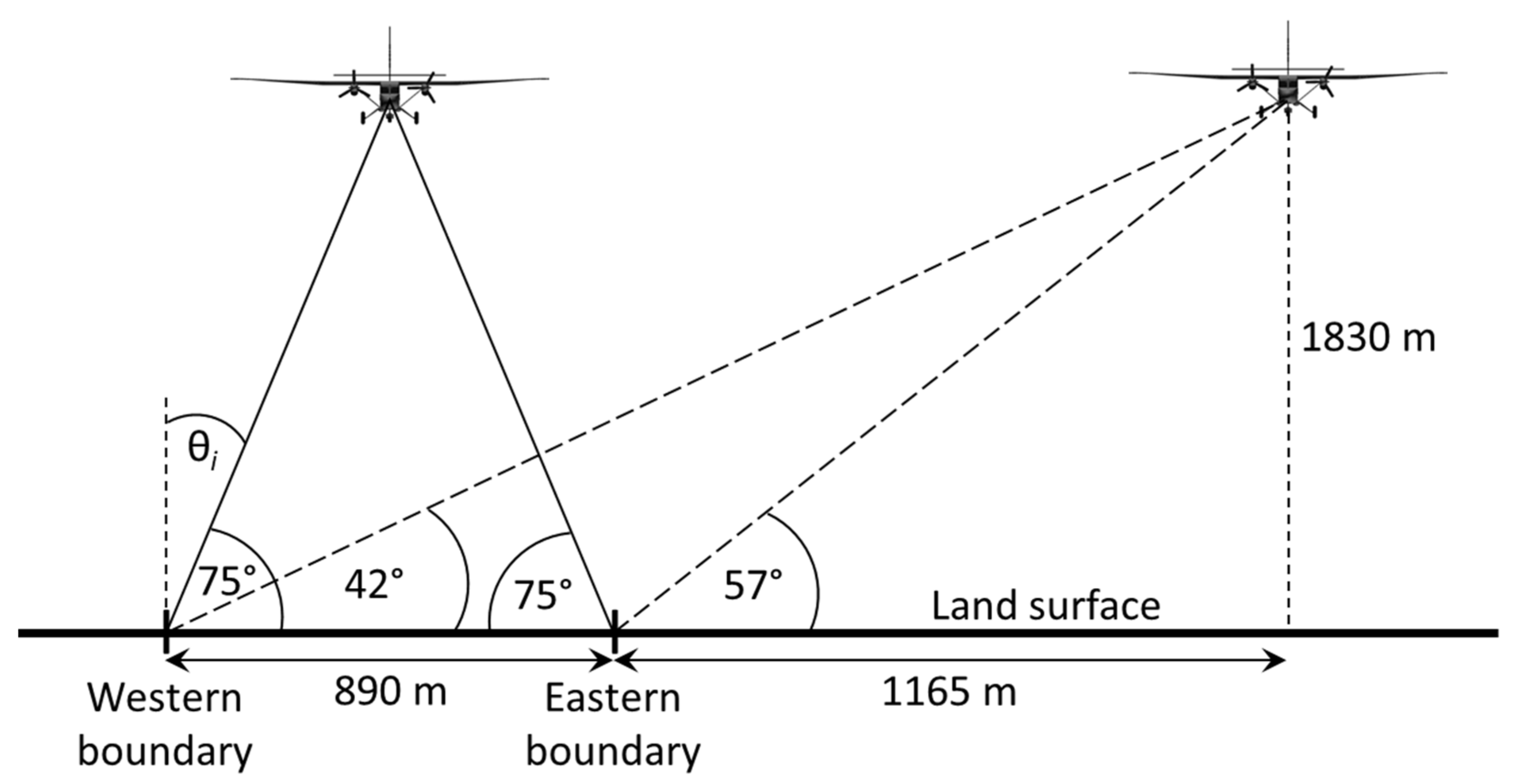
2.3. Viewing Geometries
2.4. Laboratory Spectral Measurements
3. Results
3.1. Salvia spp.
3.2. Persea americana
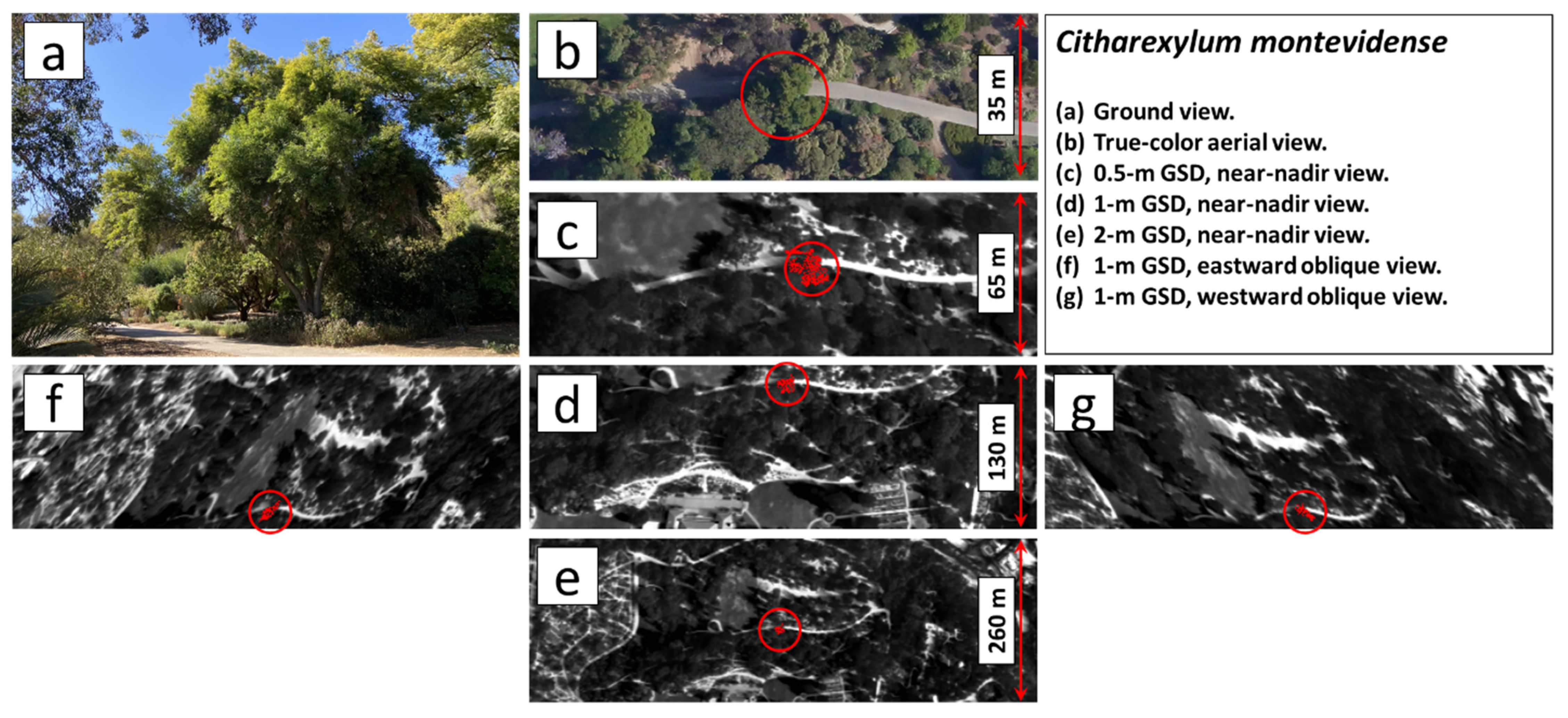
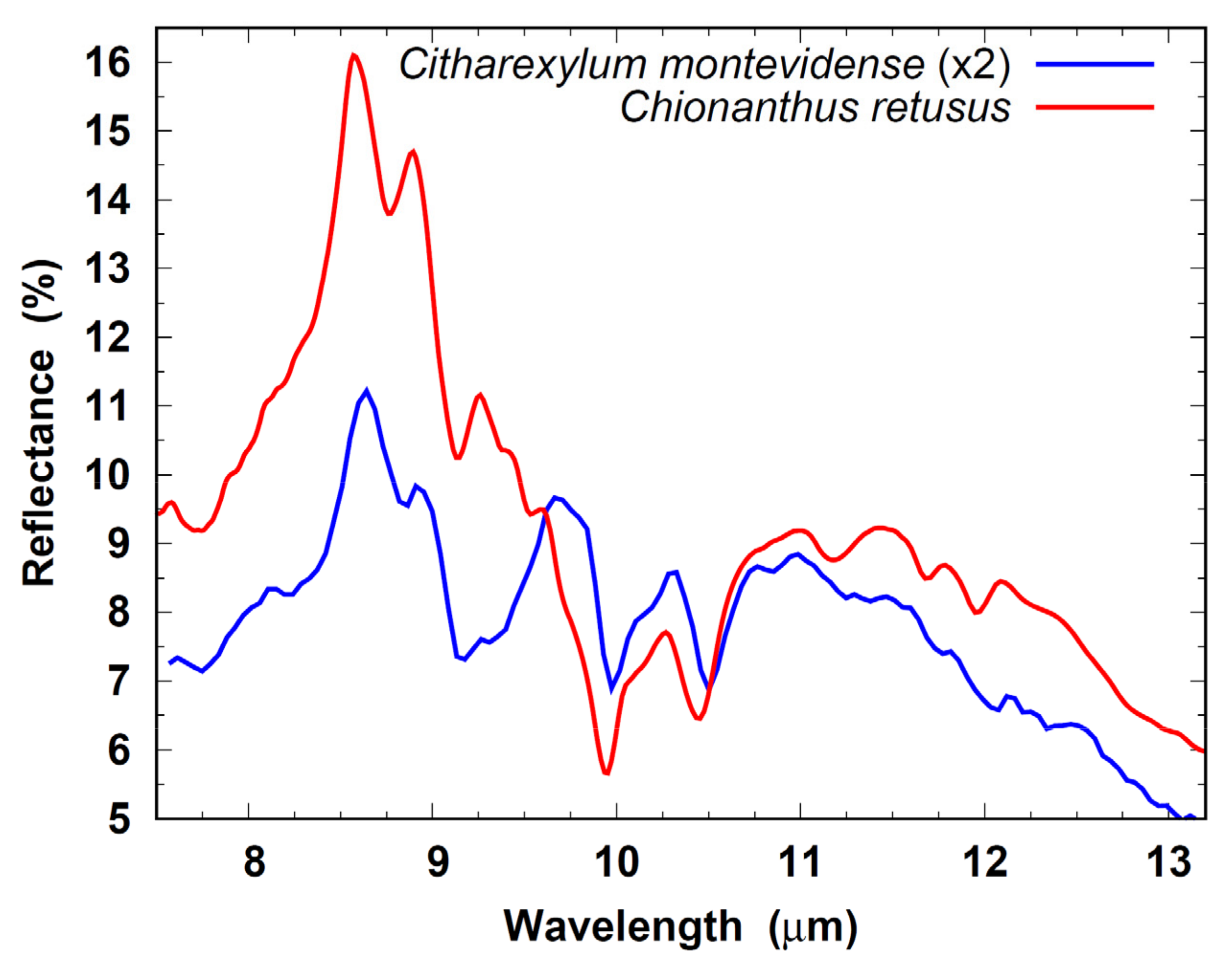
3.3. Chionanthus spp. and Citharexylum spp.
3.4. Chorisia spp.
3.5. Platanus spp.
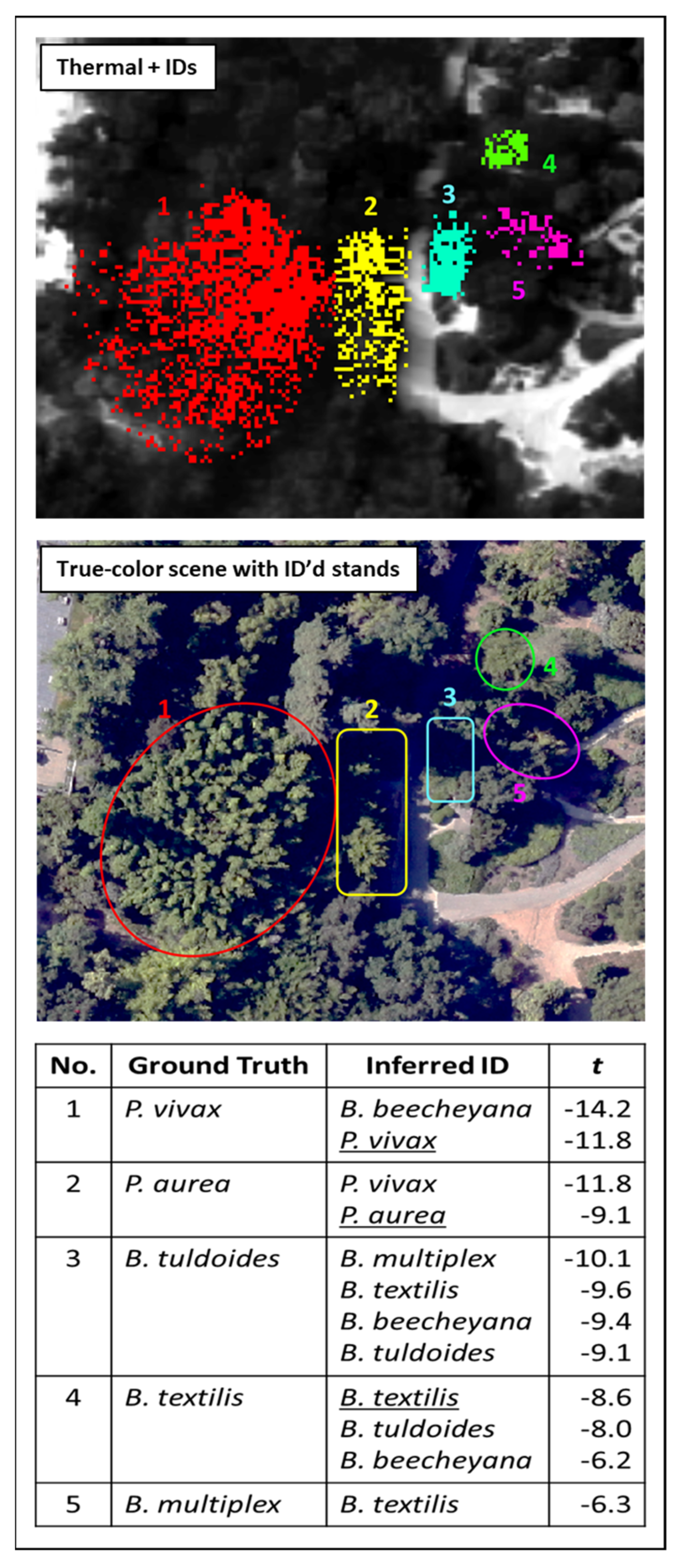
3.6. Bambusoideae
3.7. Quercus spp.
3.8. Magnolia grandiflora
3.9. Brachychiton discolor
4. Discussion
5. Conclusions
Author Contributions
Funding
Acknowledgments
Conflicts of Interest
References
- Asner, G.P.; Martin, R.E. Airborne spectranomics: Mapping canopy chemical and taxonomic diversity in tropical forests. Front. Ecol. Environ. 2008, 7, 269–276. [Google Scholar] [CrossRef] [Green Version]
- Hestir, E.L.; Khanna, S.; Andrew, M.E.; Santos, M.J.; Viers, J.H.; Greenberg, J.A.; Rajapakse, S.S.; Ustin, S.L. Identification of invasive vegetation using hyperspectral remote sensing in the California Delta ecosystem. Remote Sens. Environ. 2008, 112, 4034–4047. [Google Scholar] [CrossRef]
- Tang, L.; Shao, G. Drone remote sensing for forestry research and practices. J. For. Res. 2015, 26, 791–797. [Google Scholar] [CrossRef]
- Fassnacht, F.E.; Latifi, H.; Stereńczak, K.; Modzelewska, A.; Lefsky, M.; Waser, L.T.; Straub, C.; Ghosh, A. Review of studies on tree species classification from remotely sensed data. Remote Sens. Environ. 2016, 186, 64–87. [Google Scholar] [CrossRef]
- Meerdink, S.K.; Roberts, D.A.; King, J.Y.; Roth, K.L.; Dennison, P.E.; Amaral, C.H.; Hook, S.J. Linking seasonal foliar traits to VSWIR-TIR spectroscopy across California ecosystems. Remote Sens. Environ. 2016, 186, 322–338. [Google Scholar] [CrossRef]
- Fang, F.; McNeil, B.E.; Warner, T.A.; Maxwell, A.E.; Dahle, G.A.; Eutsler, E.; Li, J. Discriminating tree species at different taxonomic levels using multi-temporal WorldView-3 imagery in Washington DC, USA. Remote Sens. Environ. 2020, 246, 111811. [Google Scholar] [CrossRef]
- Xu, K.; Tian, Q.; Zhang, Z.; Yue, J.; Chang, C.-T. Tree species (genera) identification with GF-1 time-series in a forested landscape, Northeast China. Remote Sens. 2020, 12, 1554. [Google Scholar] [CrossRef]
- Roberts, D.A.; Ustin, S.L.; Ogunjemiyo, S.; Greenberg, J.; Dobrowski, S.Z.; Chen, J.; Hinckley, T.M. Spectral and structural measures of northwest forest vegetation at leaf to landscape scales. Ecosystems 2004, 7, 545–562. [Google Scholar] [CrossRef]
- Clark, M.L.; Roberts, D.A.; Clark, D.B. Hyperspectral discrimination of tropical rain forest tree species at leaf to crown scales. Remote Sens. Environ. 2005, 96, 375–398. [Google Scholar] [CrossRef]
- Lucas, R.; Bunting, P.; Paterson, M.; Chisholm, L. Classification of Australian forest communities using aerial photography, CASI and HyMap data. Remote Sens. Environ. 2008, 112, 2088–2103. [Google Scholar] [CrossRef]
- Féret, J.-B.; Asner, G.P. Tree species discrimination in tropical forests using airborne imaging spectroscopy. IEEE Trans. Geosci. Remote Sens. 2013, 51, 73–84. [Google Scholar] [CrossRef]
- Alonzo, M.; Bookhagen, B.; Roberts, D.A. Urban tree species mapping using hyperspectral and lidar data fusion. Remote Sens. Environ. 2014, 148, 70–83. [Google Scholar] [CrossRef]
- Feng, B.; Zheng, C.; Zhang, W.; Wang, L.; Yue, C. Analyzing the role of spatial features when cooperating hyperspectral and LiDAR data for the tree species classification in a subtropical plantation forest area. J. Appl. Remote Sens. 2020, 14, 022213. [Google Scholar] [CrossRef]
- Salisbury, J.W.; Milton, N.M. Preliminary measurements of spectral signatures of tropical and temperate plants in the thermal infrared. In Proceedings of the Fifth Thematic Conference on Remote Sensing for Exploration Geology, Reno, NV, USA, 29 September–2 October 1986; ERIM: Ann Arbor, MI, USA, 1987. Available online: https://ntrs.nasa.gov/citations/19880045682 (accessed on 22 August 2021).
- Ribeiro da Luz, B. Attenuated total reflectance spectroscopy of plant leaves: A tool for ecological and botanical studies. New Phytol. 2006, 172, 305–318. [Google Scholar] [CrossRef]
- Rock, G.; Gerhards, M.; Schlerf, M.; Hecker, C.; Udelhoven, T. Plant species discrimination using emissive thermal infrared imaging spectroscopy. Int. J. Appl. Earth Obs. Geoinf. 2016, 53, 16–26. [Google Scholar] [CrossRef]
- Harrison, D.; Rivard, B.; Sánchez-Azofeifa, A. Classification of tree species based on longwave hyperspectral data from leaves, a case study for a tropical dry forest. Int. J. Appl. Earth Obs. Geoinf. 2018, 66, 93–105. [Google Scholar] [CrossRef]
- Ribeiro da Luz, B.; Crowley, J.K. Spectral reflectance and emissivity features of broad leaf plants: Prospects for remote sensing in the thermal infrared (8.0–14.0 μm). Remote Sens. Environ. 2007, 109, 393–405. [Google Scholar] [CrossRef]
- Salisbury, J.W. Preliminary measurements of leaf spectral reflectance in the 8–14 µm region. Int. J. Remote Sens. 1986, 7, 1879–1886. [Google Scholar] [CrossRef]
- Salisbury, J.W.; Milton, N.M. Thermal infrared (2.5- to 13.5-µm) direction hemispherical reflectance of leaves. Photogramm. Eng. Remote Sens. 1988, 54, 1301–1304. Available online: https://www.asprs.org/wp-content/uploads/pers/1988journal/sep/1988_sep_1301-1304.pdf (accessed on 22 August 2021).
- Ribeiro da Luz, B.; Crowley, J.K. Identification of plant species by using high spatial and spectral resolution thermal infrared (8.0–13.5μm) imagery. Remote Sens. Environ. 2010, 114, 404–413. [Google Scholar] [CrossRef]
- Warren, D.W.; Boucher, R.H.; Gutierrez, D.J.; Keim, E.R.; Sivjee, M.G. MAKO: A high-performance, airborne imaging spectrometer for the long-wave infrared. Proc. SPIE 2010, 7812, 78120N. [Google Scholar] [CrossRef]
- Hall, J.L.; Boucher, R.H.; Buckland, K.N.; Gutierrez, D.J.; Keim, E.R.; Tratt, D.M.; Warren, D.W. Mako airborne thermal infrared imaging spectrometer: Performance update. Proc. SPIE 2016, 9976, 997604. [Google Scholar] [CrossRef]
- Buckland, K.N.; Young, S.J.; Keim, E.R.; Johnson, B.R.; Johnson, P.D.; Tratt, D.M. Tracking and quantification of gaseous chemical plumes from anthropogenic emission sources within the Los Angeles Basin. Remote Sens. Environ. 2017, 201, 275–296. [Google Scholar] [CrossRef]
- Manolakis, D.; Marden, D.; Shaw, G.A. Hyperspectral image processing for automatic target detection applications. Linc. Lab. J. 2003, 14, 79–116. Available online: https://archive.ll.mit.edu/publications/journal/pdf/vol14_no1/14_1hyperspectralprocessing.pdf (accessed on 22 August 2021).
- Manolakis, D.; Pieper, M.; Truslow, E.; Cooley, T.; Brueggeman, M.; Lipson, S. The remarkable success of adaptive cosine estimator in hyperspectral target detection. Proc. SPIE 2013, 8743, 874302. [Google Scholar] [CrossRef]
- Ullah, S.; Schlerf, M.; Skidmore, A.K.; Hecker, C. Identifying plant species using mid-wave infrared (2.5–6 μm) and thermal infrared (8–14 μm) emissivity spectra. Remote Sens. Environ. 2012, 118, 95–102. [Google Scholar] [CrossRef]
- Langsdale, M.F.; Dowling, T.P.F.; Wooster, W.; Johnson, J.; Grosvenor, M.J.; de Jong, M.C.; Johnson, W.R.; Hook, S.J.; Rivera, G. Inter-comparison of field- and laboratory-derived surface emissivities of natural and manmade materials in support of land surface temperature (LST) remote sensing. Remote Sens. 2020, 12, 4127. [Google Scholar] [CrossRef]
- Langsdale, M.F.; Wooster, W.; Harrison, J.J.; Koehl, M.; Hecker, C.; Hook, S.J.; Abbott, E.; Johnson, W.R.; Maturilli, A.; Poutier, L.; et al. Spectral emissivity (SE) measurement uncertainties across 2.5–14 μm derived from a round-robin study made across international laboratories. Remote Sens. 2021, 13, 102. [Google Scholar] [CrossRef]
- Hong, H.; Preston, B. Bayesian averaging, prediction and nonnested model selection. J. Econom. 2012, 167, 358–369. [Google Scholar] [CrossRef] [Green Version]
- Meerdink, S.K.; Hook, S.J.; Roberts, D.A.; Abbott, E.A. The ECOSTRESS spectral library version 1.0. Remote Sens. Environ. 2019, 230, 111196. [Google Scholar] [CrossRef]
- MODIS UCSB Emissivity Library (Vegetation). Available online: https://icess.eri.ucsb.edu/modis/EMIS/html/vegetation.html (accessed on 22 August 2021).
- Meerdink, S.; Roberts, D.A.; Hulley, G.; Pisek, J.; Raabe, K.; King, J.; Hook, S.J. Plant species’ spectral emissivity and temperature using the hyperspectral thermal emission spectrometer (HyTES) sensor. Remote Sens. Environ. 2019, 224, 421–435. [Google Scholar] [CrossRef]
- Neinavaz, E.; Darvishzadeh, R.; Skidmore, A.K.; Groen, T.A. Measuring the response of canopy emissivity spectra to leaf area index variation using thermal hyperspectral data. Int. J. Appl. Earth Obs. Geoinf. 2016, 53, 40–47. [Google Scholar] [CrossRef]
- Meerdink, S.K. Remote Sensing of Plant Species Using Airborne Hyperspectral Visible-Shortwave Infrared and Thermal Infrared Imagery. Ph.D. Thesis, University of California, Santa Barbara, CA, USA, 2018. Available online: https://escholarship.org/uc/item/6rd9w4vc (accessed on 22 August 2021).
- Christensen, P.R.; Harrison, S.T. Thermal infrared emission spectroscopy of natural surfaces: Application to desert varnish coatings on rocks. J. Geophys. Res. Solid Earth 1993, 98, 19819–19834. [Google Scholar] [CrossRef]
- Adams, P.M.; Lynch, D.K.; Buckland, K.N.; Johnson, P.D.; Tratt, D.M. Sulfate mineralogy of fumaroles in the Salton Sea Geothermal Field, Imperial County, California. J. Volcanol. Geotherm. Res. 2017, 347, 15–43. [Google Scholar] [CrossRef]
- Ribeiro da Luz, B. Propriedades Espectrais das Plantas no Infravermelho Termal (2,5–14 μm). Ph.D. Thesis, Instituto de Biociências, Universidade de São Paulo, São Paulo, Brazil, 2005. [Google Scholar] [CrossRef] [Green Version]
- O’Brien, C.; Hiti-Bandaralage, J.; Folgado, R.; Hayward, A.; Lahmeyer, S.; Folsom, J.; Mitter, N. Cryopreservation of woody crops: The avocado case. Plants 2021, 10, 934. [Google Scholar] [CrossRef]
- Gibbs, P.E.; Semir, J.; Da Cruz, N.D. A proposal to unite the genera Chorisia Kunth and Ceiba Miller (Bombacaceae). Notes R. Bot. Gard. Edinb. 1988, 45, 125–136. [Google Scholar]
- Gibbs, P.; Semir, J. A taxonomic revision of the genus Ceiba Mill. (Bombacaceae). An. Jardín Botánico De Madr. 2003, 60, 259–300. [Google Scholar] [CrossRef]
- Nixon, K.C.; Poole, J.M. Revision of the Mexican and Guatemalan species of Platanus (Platanaceae). Lundellia 2003, 6, 103–137. [Google Scholar] [CrossRef] [Green Version]
- Henry, A.; Flood, M. The history of the London plane, Platanus acerifolia, with notes on the genus Platanus. Proc. R. Ir. Acad. Sect. B Biol. Geol. Chem. Sci. 1919, 35, 9–28. Available online: http://0-www-jstor-org.brum.beds.ac.uk/stable/20517052 (accessed on 22 August 2021).
- Piperno, D.R.; Pearsall, D.M. The Silica Bodies of Tropical American Grasses: Morphology, Taxonomy, and Implications for Grass Systematics and Fossil Phytolith Identification; Smithsonian Contributions to Botany, No. 85; Smithsonian Institution Press: Washington, DC, USA, 1998. [Google Scholar] [CrossRef]
- Shakoor, S.A.; Bhat, M.A.; Mir, S.H. Phytoliths in plants: A review. Res. Rev. J. Bot. Sci. 2014, 3, 10–24. Available online: https://www.rroij.com/open-access/phytoliths-in-plantsa-review.php?aid=33907 (accessed on 22 August 2021).
- Du, H.; Mao, F.; Li, X.; Zhou, G.; Xu, X.; Han, N.; Sun, S.; Gao, G.; Cui, L.; Li, Y.; et al. Mapping global bamboo forest distribution using multisource remote sensing data. IEEE J. Sel. Topics Appl. Earth Observ. Remote Sens. 2018, 11, 1458–1471. [Google Scholar] [CrossRef]
- Lobovikov, M.; Paudel, S.; Piazza, M.; Ren, H.; Wu, J. World Bamboo Resources: A Thematic Study Prepared in the Framework of the Global Forest Resources Assessment 2005; UN Food and Agriculture Organization: Rome, Italy, 2007; Available online: https://www.fao.org/3/a-a1243e.pdf (accessed on 22 August 2021).
- Portillo, M.; Ball, T.; Manwaring, J. Morphometric analysis of inflorescence phytoliths produced by Avena sativa L. and Avena strigosa Schreb. Econ. Bot. 2006, 60, 121–129. [Google Scholar] [CrossRef]
- Fabre, S.; Lesaignoux, A.; Olioso, A.; Briottet, X. Influence of water content on spectral reflectance of leaves in the 3-15–µm domain. IEEE Geosci. Remote Sens. Lett. 2010, 8, 143–147. [Google Scholar] [CrossRef]
- Buitrago, M.F.; Groen, T.A.; Hecker, C.A.; Skidmore, A.K. Changes in thermal infrared spectra of plants caused by temperature and water stress. ISPRS J. Photogramm. Remote Sens. 2016, 111, 22–31. [Google Scholar] [CrossRef]
- Burkholder, A.; Warner, T.A.; Culp, M.; Landenburg, R. Seasonal trends in separability of leaf reflectance spectra for Ailanthus altissima and four other tree species. Photogramm. Eng. Remote Sens. 2011, 77, 793–804. [Google Scholar] [CrossRef]
- Hesketh, M.; Sánchez-Azofeifa, G.A. The effect of seasonal spectral variation on species classification in the Panamanian tropical forest. Remote Sens. Environ. 2012, 118, 73–82. [Google Scholar] [CrossRef]
- Meerdink, S.K.; Roberts, D.A.; Roth, K.L.; King, J.Y.; Gader, P.D.; Koltunov, A. Classifying California plant species temporally using airborne hyperspectral imagery. Remote Sens. Environ. 2019, 232, 111308. [Google Scholar] [CrossRef]
- Hennessy, A.; Clarke, K.; Lewis, M. Hyperspectral classification of plants: A review of waveband selection generalisability. Remote Sens. 2020, 12, 113. [Google Scholar] [CrossRef] [Green Version]
- Neuwirthová, E.; Kuusk, A.; Lhotáková, Z.; Kuusk, J.; Albrechtová, J.; Hallik, L. Leaf age matters in remote sensing: Taking ground truth for spectroscopic studies in hemiboreal deciduous trees with continuous leaf formation. Remote Sens. 2021, 13, 1353. [Google Scholar] [CrossRef]


| Parameter | Mako |
|---|---|
| Spectral range | 7.57–13.16 μm |
| Spectral resolution (128 channels) | 44 nm |
| Instantaneous field-of-view (IFOV) | 0.55 mrad |
| Swath width (relative to nadir) | ±56° (max.) |
| NESR (10 μm, 4 co-adds) | <0.5 μW cm−2 sr−1 μm−1 |
| NEDT (10 μm, 300 K) | 0.02 K |
| Facility | Dates Imaged | Web Site |
|---|---|---|
| Huntington Botanical Gardens (San Marino, CA, USA) | 2020-06-20 2019-04-04 2013-08-28 | www.huntington.org/gardens (accessed on 22 August 2021). |
| Los Angeles County Arboretum (Arcadia, CA, USA) | 2019-04-04 | www.arboretum.org (accessed on 22 August 2021). |
| South Coast Botanic Garden (Palos Verdes, CA, USA) | 2019-03-28 | southcoastbotanicgarden.org (accessed on 22 August 2021). |
| Lacy Park (San Marino, CA, USA) | 2020-06-20 | en.wikipedia.org/wiki/Lacy_Park (accessed on 22 August 2021). |
| Descanso Gardens (La Cañada, CA, USA) | 2021-04-07 2020-06-20 | www.descansogardens.org (accessed on 22 August 2021). |
| GSD (m) | Salvia leucophylla | Citharexylum montevidense | Bambusa beecheyana | ||||||
|---|---|---|---|---|---|---|---|---|---|
| θi (deg) | t | N | θi (deg) | t | N | θi (deg) | t | N | |
| 0.5 | 4 | −10.7 | 106 | 10 | −12.1 | 375 | 1 | −13.1 | 911 |
| 1 | 9 | −9.1 | 36 | 2 | −11.8 | 127 | 7 | −13.5 | 273 |
| 2 | 4 | - | <10 | 1 | −7.3 | 31 | 3 | −10.5 | 66 |
| 1 (E) | 45 | −7.8 | 19 | 42 | −12.7 | 78 | 45 | −11.7 | 105 |
| 1 (W) | 36 | −7.9 | 20 | 41 | −12.0 | 66 | 38 | −15.0 | 172 |
| Taxon | ID Species Returned | Spectrum Source |
|---|---|---|
| Bambusa beecheyana | Bambusa beecheyana | ECOSTRESS Library |
| Bambusa oldhamii | Bambusa beecheyana Bambusa tuldoides | ECOSTRESS Library ECOSTRESS Library |
| Bambusa textilis | Bambusa tuldoides | ECOSTRESS Library |
| Bambusa tuldoides | Bambusa tuldoides Bambusa textilis | ECOSTRESS Library This work |
| Brachychiton discolor | Brachychiton discolor Quercus robur Strelitzia nicolai | ECOSTRESS Library ECOSTRESS Library MODIS-UCSB Library |
| Cassia leptophylla | Cassia leptophylla | ECOSTRESS Library |
| Chionanthus pygmaeus | Citharexylum montevidense | ECOSTRESS Library |
| Chionanthus retusus | Citharexylum montevidense Chionanthus retusus Cornus florida Pseudocidonia sinensis | ECOSTRESS Library This work USGS-VEG Library USGS-VEG Library |
| Chorisia speciosa and hybrids | Chorisia speciosa Chionanthus retusus | ECOSTRESS Library This work |
| Ficus sycomorus | Parrotia persica | USGS-VEG Library |
| Liriodendron tulipifera | Chionanthus retusus Chorisia speciosa | This work ECOSTRESS Library |
| Magnolia grandiflora | Magnolia grandiflora | ECOSTRESS Library |
| Persea americana | Persea americana Quercus robur | This work ECOSTRESS Library |
| Platanus racemosa | Persea americana Platanus occidentalis Acer ‘Red Star’ Caesalpinia cacalaco Quercus lobata Quercus robur ssp. pedunculiflora * | This work USGS-VEG Library MODIS-UCSB Library ECOSTRESS Library ECOSTRESS Library USGS-VEG Library |
| Platanus x acerifolia | Caesalpinia cacalaco | ECOSTRESS Library |
| Quercus agrifolia | Bambusa beecheyana | ECOSTRESS Library |
| Salvia clevelandii | Salvia leucophylla | ECOSTRESS Library |
| Salvia leucophylla and hybrids | Salvia leucophylla | ECOSTRESS Library |
| Syagrus romanzoffiana | Morus alba Parrotia persica | USGS-VEG Library USGS-VEG Library |
| Ulmus parvifolia | Ficus thonningii Morus alba Ulmus carpinifolia Zelkova serrata | ECOSTRESS Library USGS-VEG Library USGS-VEG Library USGS-VEG Library |
Publisher’s Note: MDPI stays neutral with regard to jurisdictional claims in published maps and institutional affiliations. |
© 2021 by the authors. Licensee MDPI, Basel, Switzerland. This article is an open access article distributed under the terms and conditions of the Creative Commons Attribution (CC BY) license (https://creativecommons.org/licenses/by/4.0/).
Share and Cite
Tratt, D.M.; Buckland, K.N.; Keim, E.R.; Hall, J.L.; Adams, P.M.; Johnson, P.D. On the Utility of Longwave-Infrared Spectral Imaging for Remote Botanical Identification. Remote Sens. 2021, 13, 3344. https://0-doi-org.brum.beds.ac.uk/10.3390/rs13173344
Tratt DM, Buckland KN, Keim ER, Hall JL, Adams PM, Johnson PD. On the Utility of Longwave-Infrared Spectral Imaging for Remote Botanical Identification. Remote Sensing. 2021; 13(17):3344. https://0-doi-org.brum.beds.ac.uk/10.3390/rs13173344
Chicago/Turabian StyleTratt, David M., Kerry N. Buckland, Eric R. Keim, Jeffrey L. Hall, Paul M. Adams, and Patrick D. Johnson. 2021. "On the Utility of Longwave-Infrared Spectral Imaging for Remote Botanical Identification" Remote Sensing 13, no. 17: 3344. https://0-doi-org.brum.beds.ac.uk/10.3390/rs13173344