
Sentinel-2 and Landsat-8 Multi-Temporal Series to Estimate Topsoil Properties on Croplands

Institute of BioEconomy, National Research Council of Italy (CNR), Via Giovanni Caproni 8, 50145 Firenze, Italy
Remote Sens. 2021, 13(17), 3345; https://0-doi-org.brum.beds.ac.uk/10.3390/rs13173345
Submission received: 3 August 2021
/
Revised: 20 August 2021
/
Accepted: 22 August 2021
/
Published: 24 August 2021
(This article belongs to the Special Issue Multi-Sensor Data Fusion and Analysis of Multi-Temporal Remotely Sensed Imagery II)
Abstract
:The spatial and temporal monitoring of soil organic carbon (SOC), and other soil properties related to soil erosion, is extremely important, both from the environmental and economic perspectives. Sentinel-2 (S2) and Landsat-8 (L8) time series increase the probability to observe bare soil fields in croplands, and thus, monitor soil properties over large regions. In this regard, this work suggests an automated pixel-based approach to select only pure soil pixels in S2 and L8 time series, and to make a synthetic bare soil image (SBSI). The SBSIs and the soil properties measured in the framework of the European LUCAS survey were used to calibrate SOC, clay, and CaCO3 prediction models. The results highlight a high correlation between laboratory soil spectra and the SBSIs median spectra, especially for the SBSI obtained by a three-year S2 collection, which provides satisfactory results in terms of SOC prediction accuracy (RPD: 1.74). The comparison between S2 and L8 results demonstrated the higher capability of the S2 sensor in terms of SOC prediction accuracy, mainly due to the greater spatial resolution of the bands in the visible region. Whereas, neither S2 nor L8 could accurately predict the clay and CaCO3 content. This is because of the low spectral and spatial resolution of their SWIR bands that prevent the exploitation of the narrow spectral features related to these two soil attributes. The results of this study prove that large S2 time series can estimate and monitor SOC in croplands using an automated pixel-based approach that selects pure soil pixels and retrieves reliable synthetic soil spectra.
Keywords:
time series; multi-temporal; mosaicking; bare soil; SOC; clay; CaCO3; LUCAS; Sentinel-2; Landsat-8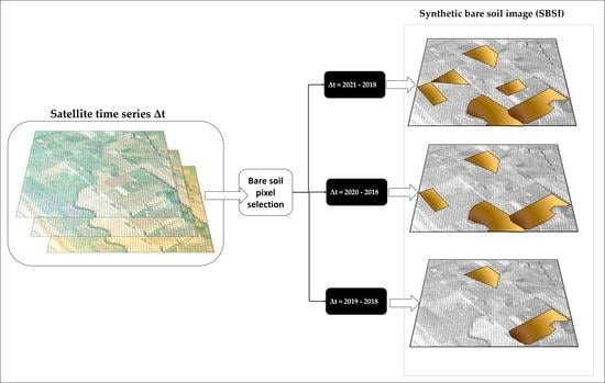
1. Introduction
Soil organic matter loss, and consequently soil erosion, is one of the main processes of land degradation in croplands, often due to increasingly intensive agricultural management [1,2]. In this regard, The Voluntary Guidelines for Sustainable Soil Management published by Intergovernmental Technical Panel on Soils [3] indicated the loss of soil organic carbon (SOC) as one of the main causes of soil degradation and lay down a set of good practices to enhance the soil organic matter content and improve the soil fertility. These practices will be used as guidelines for cross-compliance rules for Common Agricultural Policy (CAP) related to the good agricultural and environmental condition (GAEC) of the land for the period post-2020 [4].
Other soil properties like topsoil clay, sand, and calcium carbonate (CaCO3) can be used to quantify the soil vulnerability in terms of erosion [5,6]. Consequently, spatial and temporal monitoring of SOC and other soil properties related to soil erosion is extremely important, both from the environmental and economic perspective for sustainable soil management within the European Green Deal, that aims to reduce the misuse of fertilizers, and at the same time, to increase the carbon stock in the soil [7,8].
The physical link between soil properties and the electromagnetic spectrum in the optical spectral domain is well-known [9], and widely exploited in soil spectroscopy for soil properties estimation and monitoring [10]. This is due to chemical components or chromophores interacting with visible and infrared radiations and showing well-defined absorption features [11]. Clay minerals have typical spectral features in the short waves infrared region (SWIR) between 2170 and 2360 nm, corresponding to metal-OH bends and O-H stretch [12,13]. Calcium carbonate (CaCO3) has an absorption peak in the SWIR region around 2348 nm corresponding to CO3 overtone vibrations [14]. Due to the heterogeneity of the organic matter components, SOC has not spectral features in narrow spectral regions; however, it shows a relationship with electromagnetic radiation both in the visible region around 450, 590, and 664 nm [9], in the near-infrared (NIR) and SWIR region, principally due to the two main organic compounds that affect the reflectance: Lignin (between 1600 and 1800 nm and around 2100 nm) and cellulose (around 2100) [9]. Laboratory spectra usually cover the whole optical domain (400–2500 nm) with a high spectral resolution (≤2 nm)—this fully exploits the narrow spectral features linked to soil variables. However, the strength of the relationships between spectral features and soil properties decreases from laboratory to satellite imaging spectroscopy [11]. This is due to the combination of several factors linked with the sensor characteristic (range and spectral resolution) and the distance between the sensor and target surface (atmospheric disturbance, signal quality, spectral and spatial resolution), and the soil surface conditions (moisture, roughness, vegetation residues). Despite this, many recent scientific papers demonstrated the capability of the Copernicus Sentinel-2 Multi-Spectral Instrument (MSI) (hereinafter referred to as S2) and NASA Landsat-8 Operational Land Imager (OLI) (hereinafter referred to as L8) optical data for soil properties prediction and mapping [15,16,17,18,19,20,21], obtaining encouraging results, especially for the SOC content.
The short revisit time of the S2 (five days) and L8 (sixteen days) constellations increases the likelihood to observe cloud-free images and a large number of bare soil fields, this is especially important in the soil imaging spectroscopy context, for the narrow time window in which we can find bare soil in croplands. In this regard, the collection of multi-temporal data for the same area can increase the mapped area by mosaicking several images. The mosaicking process makes a composite or synthetic bare soil image [22,23,24,25,26] that can also be useful to plan a soil sampling that considers all the soil variability in a certain region exploiting the link between spectral characteristics and soil properties [27]. However, in case of non-availability of a robust IT infrastructure with large storage capability and high computing power, a cloud platform that offers catalogs of satellite imagery and geospatial analysis capabilities by an Application Programming Interface (API) is necessary to analyze this plethora of available data within a large time series in a most effective way. In this regard, Google Earth Engine [28] was successfully employed for obtaining a bare Earth’s surface spectra using L8 multi-temporal data [29].
However, one of the main challenges for automating the soil properties mapping and monitoring from multispectral satellite data is the minimization of disturbing factors, such as green and dry vegetation, roughness, and soil moisture. These disturbing factors influence the interpretation of the spectra acquired by remote sensing, especially for images with low or medium spatial resolution, such as those provided by S2 and L8, which involve the presence of mixed pixels, i.e., pixels containing more than one distinct material, thus not only soil or vegetation [17,20,23]. To attract new users and exploit the benefits of the S2 and L8 data, we need to clearly define the conditions under which prediction models can be developed and applied to produce reliable soil properties maps over a large area. This includes developing algorithms for detecting bare soils in croplands excluding mixed spectra and minimizing the disturbing factors. Ideally, the soil properties model should be built and applied using the spectral information derived from pixels on bare soil without green or dry vegetation and mimicking the conditions of a dry soil sample with a reduced roughness (e.g., soil in seedbed condition) [17,20,23].
This work suggests an automated pixel-based approach to select only exposed soil pixels (pure soil pixels) not strongly affected by disturbing factors in the large satellite image collection. The proposed method was applied both to the S2 and L8 time series available in the GEE platform with the aim of investigating how the time interval width affects the accuracy of the SOC, clay, and CaCO3 estimation models. For these purposes, the SBSIs were obtained using images acquired in three different time windows (1, 2, and 3 years), both for S2 and L8 images, and the soil samples collected for the 2015 LUCAS topsoil survey were used to build multivariate regression models.
2. Materials and Methods
2.1. LUCAS Topsoil Dataset
In the framework of the Land Use and Coverage Area frame Survey (LUCAS), a topsoil survey is carried out in the Member States of the European Union (EU) every three years to collect statistical information on soil properties. The 2015 LUCAS database includes soil samples for all the 28 countries of the EU, and it was carried out over 90% of the locations sampled in the earlier surveys (2009 and 2012), while the remaining 10%, 5656 samples, were collected over new locations [30].
All the soil samples from the LUCAS surveys in 2009, 2012, and 2015 were collected following the same standard protocol that entails the collection of a composite sample (about 500 g and 20 cm depth) taken by a spade in five points: The first point corresponds to the point location and the other four at 2 m distance following the cardinal directions [31].
Thirteen chemical and physical parameters were measured in the laboratory for each soil samples from the 2015 LUCAS topsoil database, by the ISO methods (clay [32]; organic carbon [33]; calcium carbonate [34]).
The spectra were acquired with an XDS Rapid Content Analyzer (FOSS NIR Systems Inc., Laurel, MD, USA) spectrometer between 400 and 2500 nm with 2 nm resolution following the protocol described by [35].
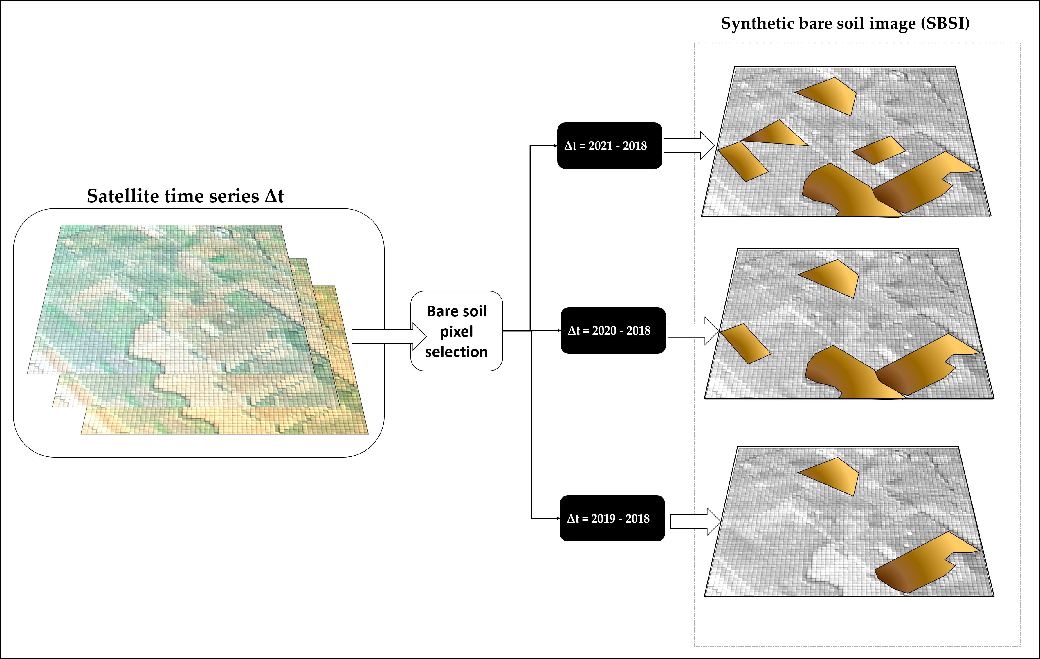
To link the most recent and available LUCAS soil data with satellite images, and to avoid exceeding the user memory limit imposed by GEE, some regions across Europe were selected, where 815 soil samples were collected in new locations in croplands during the 2015 LUCAS survey: Great Britain and Ireland, Central Europe (Germany, Austria, Czech Republic, Slovakia, Hungary, and Poland), Baltic states (Latvia, Lithuania, Estonia), Western Europe (Great Britain, Ireland, Belgium, Netherlands, Luxembourg, and South France), and Southern Europe (Italy and Malta) (Figure 1).
2.2. Satellite Multi-Temporal Series to Select Bare Soil
Synthetic bare soil images (SBSI) were obtained in the GEE environment by a pixel-based multi-temporal analysis using S2 level 2A (COPERNICUS/S2_SR in GEE) and L8 level 2, collection 2, Tier 1 (LANDSAT/LC08/C02/T1_L2 in GEE) images collections.
Different time intervals were investigated for the satellite collections:
- From May 2018 to May 2021, both for S2 and L8: hereinafter referred to as S2_3Y and L8_3Y
- From May 2019 to May 2021, both for S2 and L8: hereinafter referred to as S2_2Y and L8_2Y
- From May 2020 to May 2021 both for S2 and L8: hereinafter referred to as S2_1Y and L8_1Y
- From May 2015 to May 2016 just for L8: hereinafter referred to as L8_1Y_L.
The 1Y_L collection was added to have satellite data close to the LUCAS survey period—unfortunately S2 was not yet available.
The selection of the bare soil pixels for each image of the collection was carried out in the selected regions concerned by the new sampling location of the 2015 LUCAS survey.
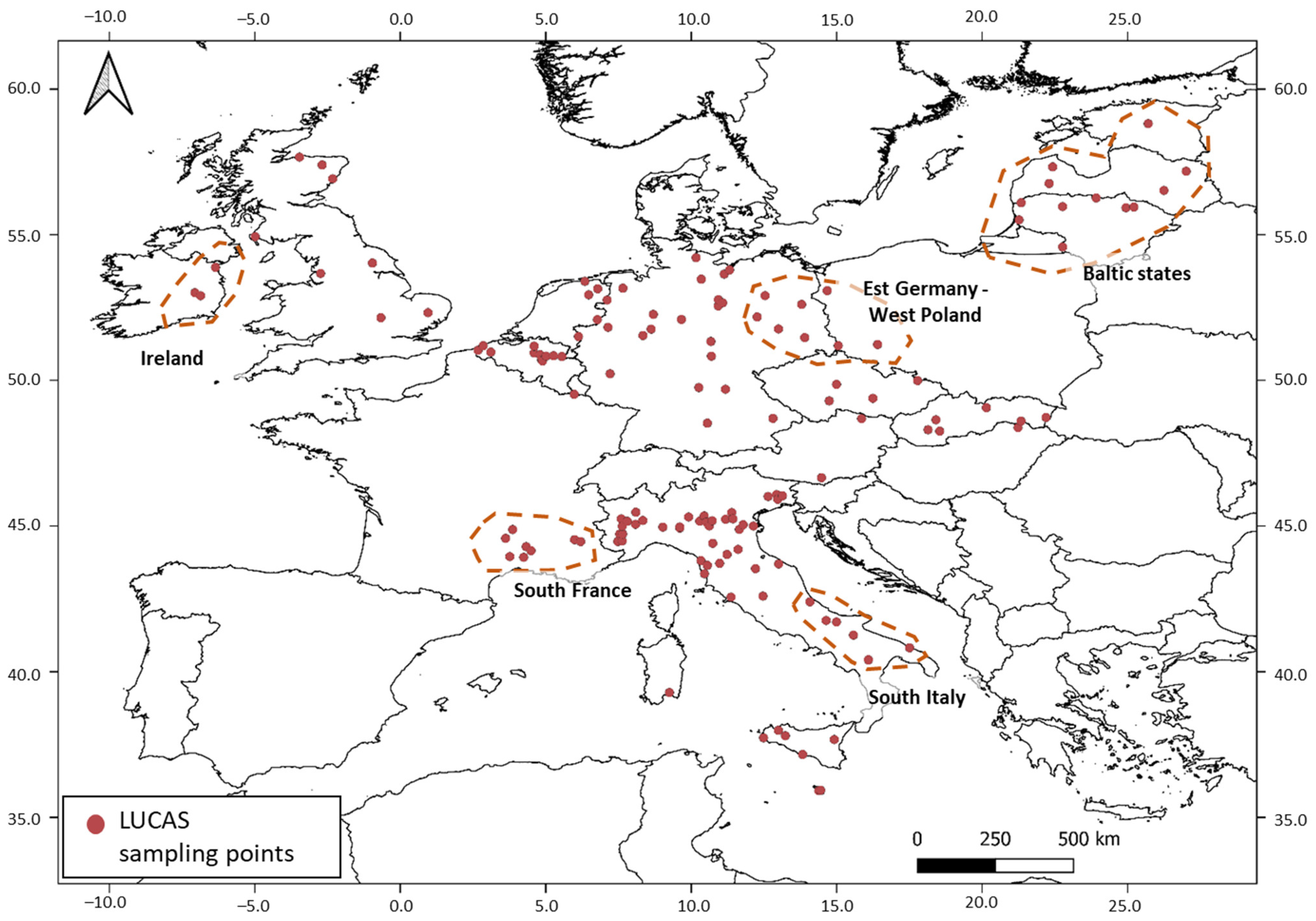
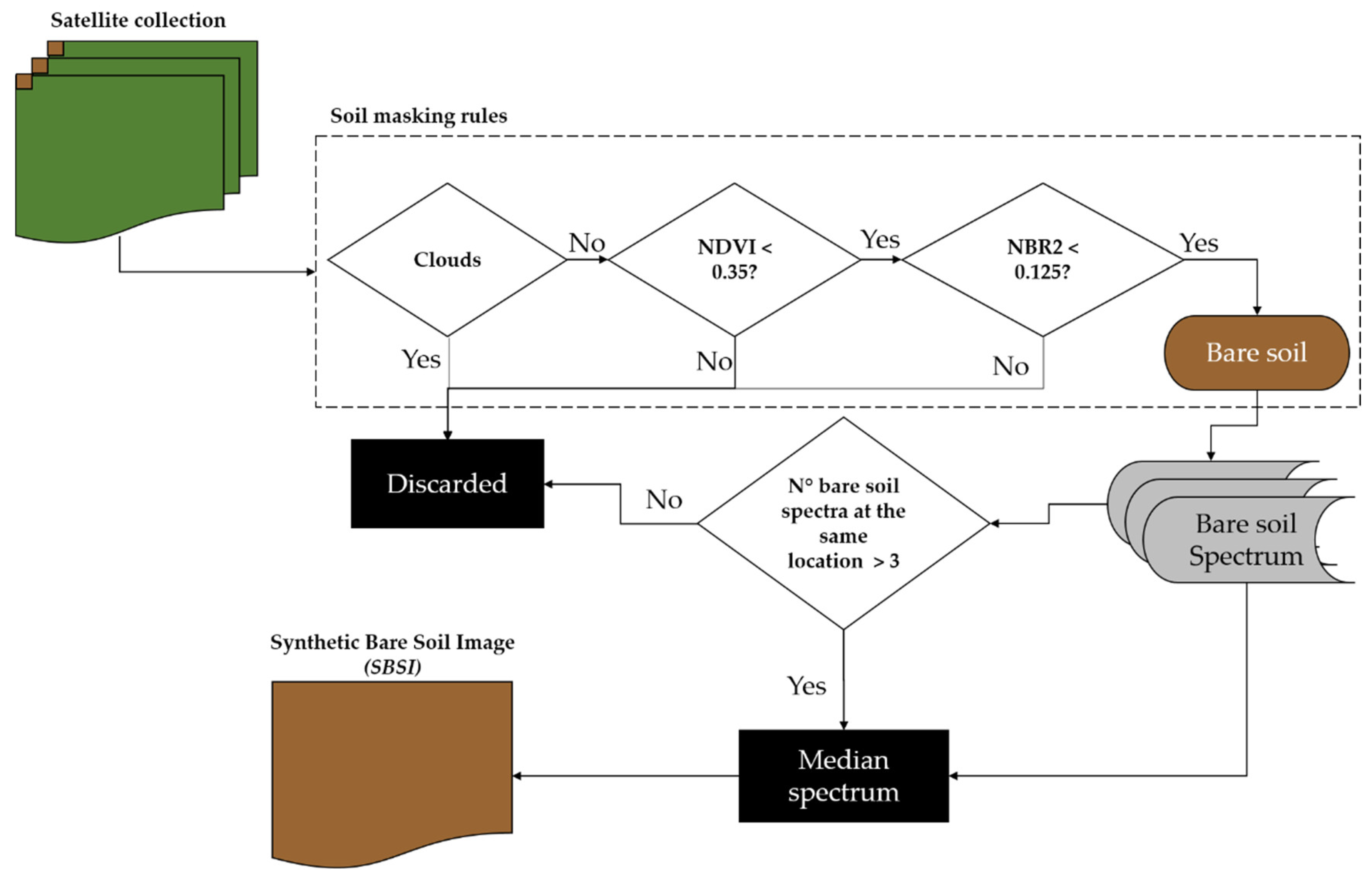
This selection entails applying a cloud mask removing pixel affected by clouds and clouds’ shadows using the products included in the two satellite collections. The ‘QA60 Sentinel-2 bitmask band with cloud mask information was used to mask cirrus and opaque clouds, and the ‘MSK_CLDPRB’ and ‘MSK_SNWPRB’ bands were used to remove cloudy and snowy pixels, respectively. The Pixel Quality Assessment Band provide by L8 was used to mask cloudy pixels.
After that, the Normalized Difference Vegetation Index (NDVI) and Normalized Burn Ratio 2 (NBR2) Equation (1) indices were computed for the remaining pixels to detect green and dry vegetation, respectively,
The SWIR1 band corresponds to B6 for L8 and B11 for S2, while SWIR2 to B7 for L8 and B12 for S2 (Table 1). The NBR2 index can also remove pixels interested by high soil moisture content that can affect the soil spectrum shape [22]. Only the pixels which comply with the following conditions: No clouds, NDVI < 0.35, NBR2 < 0.125 were kept. The NDVI and NBR2 thresholds were set according to a conservative approach that aims to find a compromise between the size of the dataset and the estimation accuracy [17,23]. For each geographical location represented by the center of the satellite pixel, we could get several dates complying with the above-mentioned conditions. Therefore, we computed the median value for each band, but only considering the locations that respect all the conditions at least three times within the time series (Figure 2). The selected bands for S2 and L8 data are listed in Table 1.
The final output is a synthetic bare soil image (SBSI) for each time interval both for S2 (3Y, 2Y, 1Y) and L8 (3Y, 2Y, 1Y, 1Y_L).
To demonstrate the role of the time series to increase the SBSIs area and their reliability for soil properties mapping, four representative areas of interest from the 2015 LUCAS survey were selected: Baltic states, Ireland, South Italy, and East Germany-West Poland (Figure 1). For each sampling location in these areas, we counted how many times the corresponding pixel complying with the conditions described above—in other words, the bare soil frequency within a time interval for the same point.
2.3. Soil Properties Estimation Models
The SOC, clay, and CaCO3 content provided by the 2015 LUCAS survey and the median spectrum of the SBSIs were used to build the prediction models using the Cubist algorithm. The Cubist is a predicted-oriented regression algorithm with a unique linear regression model at each node defined by a rule. The rules concern the predictors, here the reflectance values of the satellite bands, defining a subset at each node that makes a multi-way tree structure [36]. The Cubist [37] and caret R packages were used to tune the models to find the best number of neighbors and committees (boosting iterations) that minimizes the 10-fold cross-validation root mean square error (RMSE). To compare the accuracy obtained in this work for the three soil properties and with other results in the literature, the ratio of performance to deviation (RPD) Equation (2), were computed,
where std is the standard deviation of the observed values.
The LUCAS soil properties values were also used with laboratory spectra to build estimation models that can be used as the reference test, since laboratory spectral data should represent the best condition for soil properties estimation, where there are no disturbing effects, due to the distance between sensor and target and the roughness is negligible. In this case, due to the high number of predictors (bands), the well-known partial least squares regression (PLSR) algorithm was also tested [38], which has proved to be powerful for hyperspectral data in soil spectroscopy [39,40]. Cubist and PLSR models were tested for all satellite and laboratory datasets, and only the best result of the two was reported. Moreover, the laboratory spectra were resampled using Gaussian models, according to the L8 (Lab_L8) and S2 (Lab_S2) central wavelengths and bandwidths listed in Table 1.
3. Results
3.1. Bare Soil Selection
Obviously, the larger the time interval, higher the number of bare soil pixels in all the selected regions (Table 2). The 3Y collection generally avoids very low bare soil frequency, especially for the S2 time series. The highest average values were detected in South Italy and East Germany–West Poland, where the S2 time series provides more bare soil pixels than the L8 collection. The lowest number of bare soil pixels was obtained in the Ireland region, mainly due to the high cloudiness.
3.2. LUCAS Subset
Table 3 shows the descriptive statistics of the soil samples (Figure 1), for which it was possible to retrieve a median bare soil spectrum both for the S2 and L8 time series. Although the number of available samples decreases using a narrower time interval (from 3Y to 1Y), the range, mean, and standard deviation only vary slightly. All three soil properties have a very large range of values and high variability. These datasets were used to build clay, SOC, and CaCO3 prediction models.
3.3. SOC, Clay, and CaCO3 Estimation Accuracy
The accuracy of the models calibrated using laboratory spectra (Lab) is very high for CaCO3 (RPD: 2.74) and lower for clay (RPD: 1.83) and SOC (RPD: 1.58). Resampling the laboratory spectra according to the S2 and L8 spectral characteristics, the accuracy decreases for all the three soil properties, and, in particular, for CaCO3, for which the RMSE is almost doubled (Table 4). The models calibrated with the S2 data showed a good estimation accuracy for SOC content, especially using the S2_3Y time series (RPD: 1.74), while the RPDs of clay and CaCO3 are quite low. The SOC model using the L8_3Y data provided a sufficient degree of accuracy (RPD: 1.53), however all the L8 statistics are worse than those obtained by S2 data. Generally, the 3Y models provided the best results, while the use of the L8_1Y_L collection did not show any advantage in terms of estimation accuracy as compared to 1Y.
4. Discussion
Vegetation in cropland fields persists most of the time during the year. Consequently, the probability of acquiring a clouds free image and to find, at the same time, bare soil is quite low. In this regard, the composite image increases the investigated area for soil properties mapping, especially if a long and large time series collection is available, such as that provided by the Landsat program, and in particular Landsat-5 (started in 1984), Landsat-7, and the most recent Landsat-8 mission. In this regard, Demattê et al. [23] used Landsat 5 collection to obtain a synthetic soil image of the Sao Paulo region in Brazil, Demattê et al. [29] obtained bare Earth’s surface spectra based on Landsat series, and Safanelli et al. [41] used 37 years Landsat data to map soil properties in Europe. Although Sentinel-2 constellation delivered the first images in 2015, the short revisit time provided by the Sentinel-2 already collects a large amount of data worldwide, and some authors started to explore the capability of the S2 time series. These authors include Vaudour et al. [26], who used S2 time series to map SOC in the Versailles plain in France, and Silvero et al. [42], who combined S2 and L8 time series for soil mapping purposes over large areas.
Table 2 showed how the better S2 revisit time (five days), as compared with that of L8 (sixteen days), entails collecting more bare soil pixels at the same location, and consequently, obtaining more reliable median reflectance values, smoothing the effect of extreme values. Moreover, collecting images across more years increases the probability of including a larger number of exposed soils in the SBSI, thus increasing the mapping area in croplands. This is particularly important in regions where it is more difficult to acquire clear-sky images, such as those of North Europe (e.g., the Baltic States and Ireland).
The number of selected pixels, classified as bare soil, depends on the criteria adopted for the selection, and thus, for the minimization of the disturbing factors. The NDVI index was widely and successfully used to discriminate between soil (NDVI < 0.25–0.35) and green vegetation, due to the sharp increase of the reflectance between red and NIR region in the vegetation spectrum, while the differences between dry vegetation (crop residues, straw, stubble, etc.) and soil are less showy. The lignin spectral feature in SWIR (around 2100 nm) could help detect dry vegetation, but it is located very close to kaolinite and other clay minerals features that characterize soil spectra. Therefore, the NBR2 has been widely used to detect dry vegetation and spectra affected by high moisture content [16,23]. This normalized index exploits the spectral region between 1600 and 2100, which is almost flat for soil spectra, while the dry vegetation curve is descending, and the slope of the curve is related to the percentage of dry vegetation [23]. The NBR2 was successfully tested both with L8 data using B6 and B7 and with S2 using B11 and B12 [17,26]. Although lower the NBR2 value, higher the probability of detecting pure soil, there is not yet a clear agreement about the best NBR2 threshold value for the discrimination, and the study of Castaldi et al. [17] suggests that the choice should be guided by the specific requirements of the study trying to find a compromise between prediction accuracy and spatial coverage of the map. Vaudour et al. [26] compared per-pixel and per-date approaches for S2 time series, and they gained the best compromise between mapped extent and SOC accuracy (RPD= 1.50) using a per-date approach selecting the driest soil based on soil surface moisture index (S2WI).
Another important disturbing factor is the soil surface roughness, which can be minimized by selecting images acquired when it is more probable to find soil in a seedbed condition. In this regard, Dvorakova et al. [20] selected the ‘greening-up’ period based on the NDVI timeline, i.e., the last date of acquisition where the NDVI is lower than 0.25 before the crop develops, and they were able to significantly improve the SOC estimation accuracy combing the ‘greening-up’ approach with a very strict NBR2 threshold (< 0.07), which, however, limited the extent of the mapping area.
If, on one the hand, the composite images increase the mapping area, then, on the other hand, soil imaging spectroscopy should use images acquired as close in time as possible to ground truth survey to build a reliable prediction model, and this assumption is not respected using large multi-temporal data. It must nevertheless be noted that most of the soil properties are quite stable, or change very slowly over time, if no drastic changes in soil management, land use, or cover occur and where there were not remarkable erosion processes or extreme meteorological events. The comparison between 2009 and 2015 LUCAS surveys in 17,613 soil points showed limited changes over the six years period [43]. Consequently, the temporal difference between soil survey and satellite data could be irrelevant for modeling and mapping purposes.
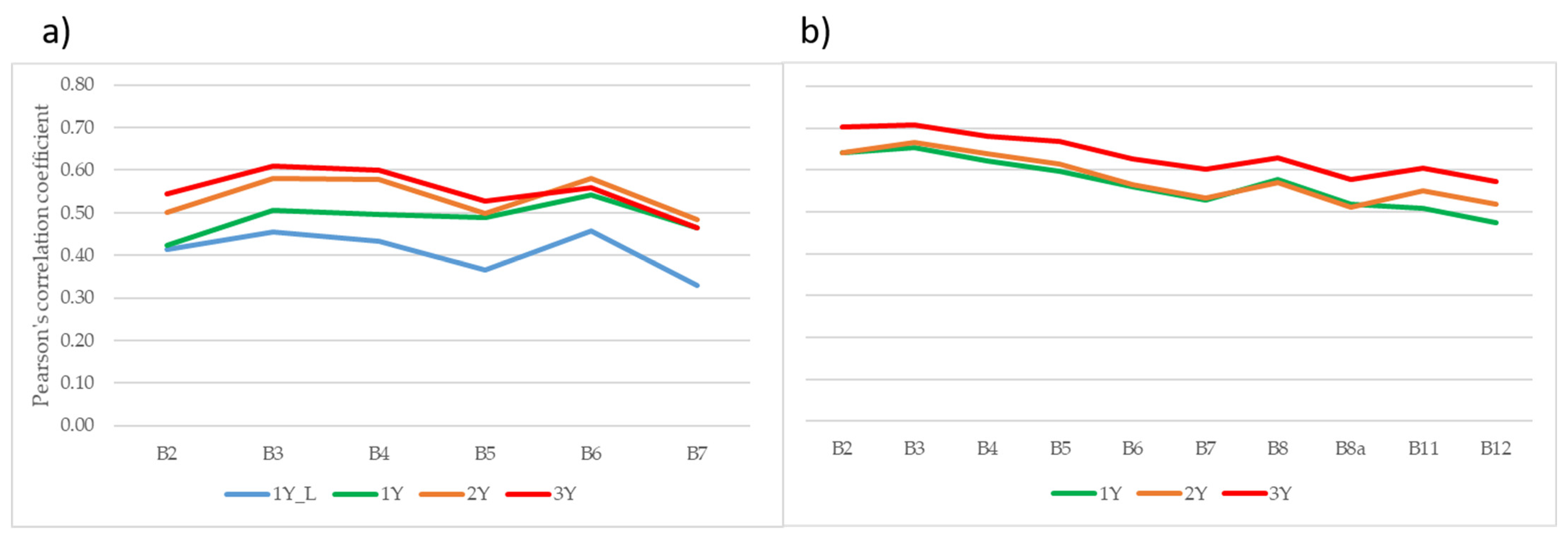
Another important aspect to consider is the consistency between survey area and pixel size or ground sampling distance (GSD). A composite topsoil sample was collected for the LUCAS survey within a circular area of 2 m radius, while the ground sampling distance (GSD) for S2 is 10 m for the visible band, and 20 m in the NIR and SWIR bands. The discrepancy between soil sampling area and GSD is even more marked for L8: All the L8 bands have a resolution of 30 m. This incongruity could lead to not reliable soil estimation models if the measured values do not represent the actual situation within the pixel area [27,44,45]; this issue may become more pronounced according to the magnitude of the geometric error and if the investigated soil property has a large short-range spatial variability. The Pearson’s correlation coefficient between reflectance measured on LUCAS soil samples in the laboratory and satellite data (Figure 3) highlighted how the S2 SBSIs are closer to lab spectra than L8 SBSIs, probably due to the lower spatial resolution of the NASA sensor.
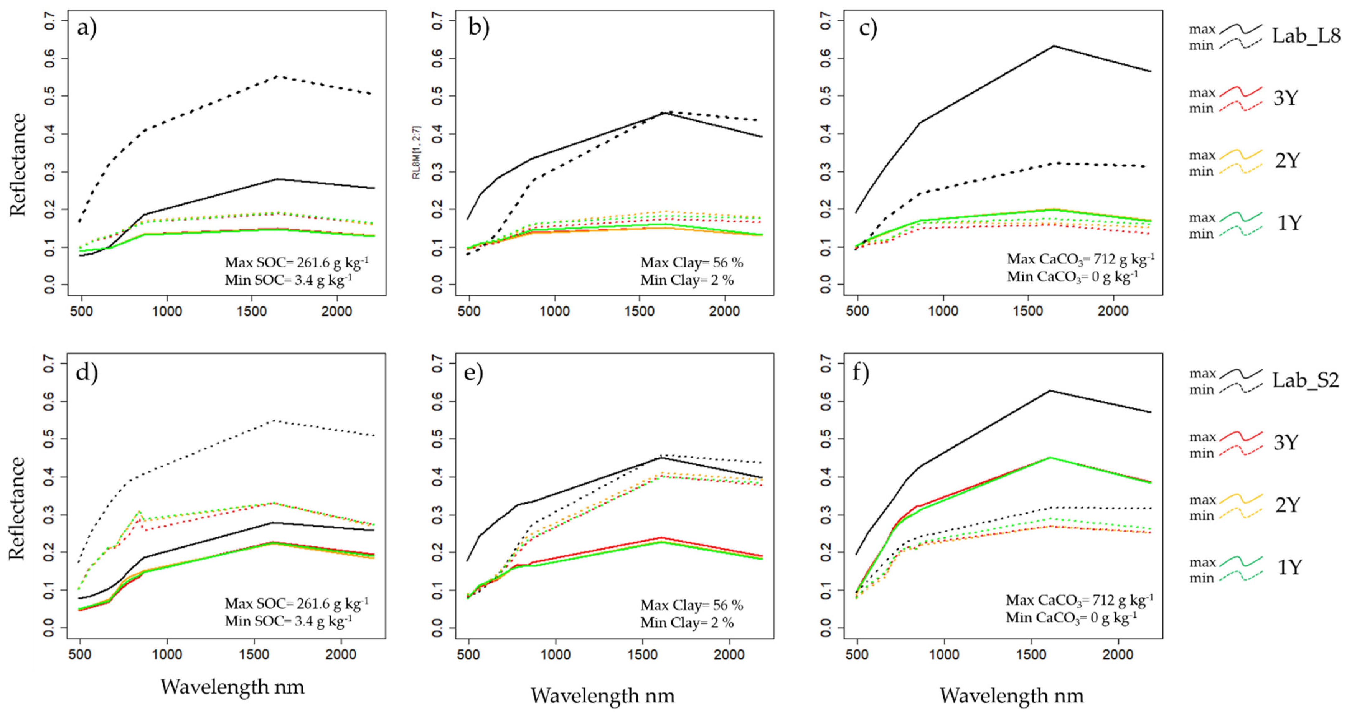
Figure 3 also shows that, in general, the correlation is stronger in the visible region and that the 3Y SBSI is more correlated to laboratory spectra than 2Y and 1Y for all the S2 bands and for B2, B3, B4, and B5 of the L8. These outcomes are consistent with [41] that using L8 found that generating a bare soil composite image by using a time interval close in time to soil observations did not improve neither the quality of topsoil reflectance nor the prediction accuracy of soil properties, especially for the more stable soil attributes, such as clay and CaCO3. Observing Table 4, it is quite evident how the highest accuracy was obtained using 3Y SBSI, especially for SOC estimation. Thus, both the correlation investigation and the model accuracy demonstrated that a large time interval leads to a more reliable SBSI, probably because it can reduce the negative effect of extreme estimates along with the multi-temporal survey [41]. Figure 4 shows how the S2 SBSI spectra are quite similar to laboratory spectra for high SOC content and low clay and CaCO3 (Figure 4d–f). The observed differences between laboratory and satellite spectra in terms of reflectance value are probably due to soil moisture that reduces the reflectance over the entire spectrum, influencing the amount of reflected and emitted energy from a soil surface [13,46]; the LUCAS soil samples were dried before being scanned in the laboratory, while the satellite spectra, although the NBR2 was applied to exclude high soil moisture content, still retain a certain amount of water especially for soil with a high clay content. As proof of the previous sentence, we have shown the difference between Lab_S2 and the satellite spectrum is bigger for very high clay content than for low content (Figure 4e).
The L8 spectra in Figure 4a,b and c clearly highlights how the reflectance of the synthetic curves is greatly lower than laboratory spectra both for high and low SOC, clay, and CaCO3 contents—their shape is quite flat and the reflectance values are relatively low (most of them around 0.1). The 30 m spatial resolution of the L8 bands increases the probability to include more than one element within the pixel area (e.g., vegetation and soil), and at the same time, this entails a lower capability to detect the presence of the two main elements using the spectral behavior [47,48]; in other words, the NDVI, or other indices, could be not able to discriminate between pure soil and mixed pixels and this could lead to include not bare soil spectra in a time series. However, the effect of these mixed spectra can be mitigated by the computation of the median spectra along with the time series.
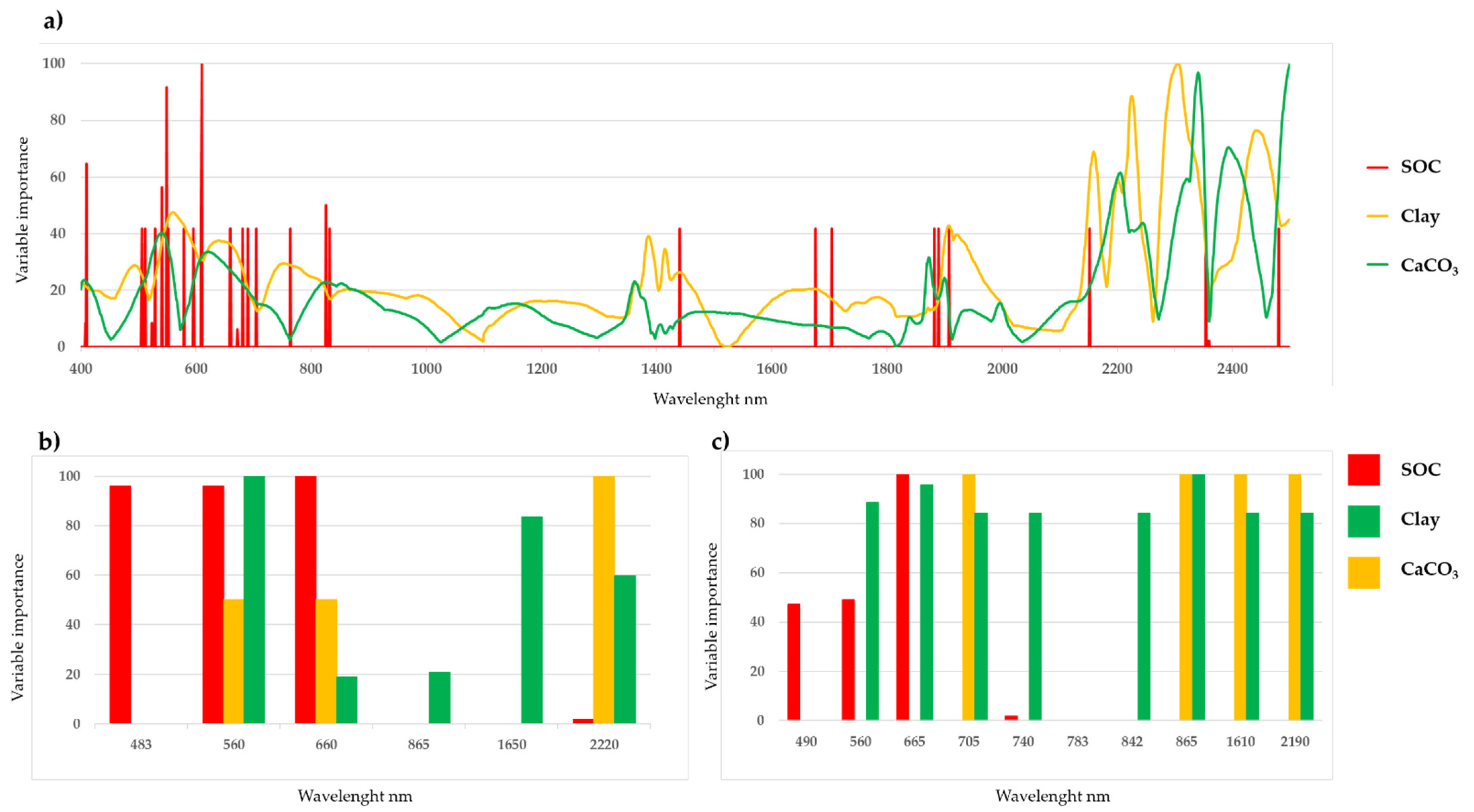
The prediction models calibrated with laboratory spectra provided a good accuracy for all the three soil properties, and, in particular, the CaCO3 showed a very high RPD (2.74). The resampling process according to the S2 and L8 bands highlighted how a high spectral resolution is needed for clay and calcium carbonates estimation, while it seems less important for SOC. This agrees with the observations from the authors of [49] that noted that the reduction of spectral resolution has not a remarkable effect on SOC estimation accuracy, while for a bandwidth larger than 40 nm, the clay estimation accuracy decreases significantly. The authors of [15] and [16] compared Sentinel-2 and airborne hyperspectral data in terms of SOC estimation accuracy. Both papers concluded that Sentinel-2 estimates and maps SOC, and that the retrievable accuracy is not significantly different than that obtained by a better spectral and spatial resolution—especially where a large SOC variability is observable. Whereas, for clay and CaCO3 estimation, only narrow bands can exploit the spectral features related to these two properties, the heterogeneity of the organic matter composition entails a spectral response spread over the whole electromagnetic spectrum and not limited to a specific spectral region. The clay and CaCO3 spectral features are located in the SWIR region. Figure 5 clearly shows that the most important bands for clay and CaCO3 Lab models are located between 2100 and 2500 nm and only a few bands in the visible (Figure 5a).
The variable importance analysis for 3Y SBSI models confirmed the trend, described above (Figure 5b,c). However, despite both S2 and L8 have two bands in this SWIR, the clay and CaCO3 prediction accuracy is much lower than that observed with laboratory data, this is due on the one hand to the large bandwidth of the S2 and L8 SWIR bands (between 85 and 187 nm), that does not properly exploit the narrow spectral feature of the clay mineral and those related to CaCO3, and on the other hand to the large pixel size of these bands (20 m for S2 and 30 m for L8). The most important bands for SOC prediction are mostly located in the visible region (Figure 5a), this is also clear for 3Y SBSI models both for L8 and S2, where basically only the blue, green, and red bands contribute to the cubist models (Figure 5b,c). Therefore, the higher accuracy of the satellite SOC models can be explained by the better spatial and spectral resolution (10 m and bandwidth between 30 and 65 nm) of the S2 visible bands compared with SWIR bands. The importance of the resolution of the S2 visible bands can be confirmed by the high correlation between laboratory and satellite spectra shown in Figure 3b: Around 0.7 for 3Y image and around 0.65 for 2Y and 1Y. As shown in Table 4, it should be noted that S2 provided a better SOC prediction accuracy than L8—probably due to the higher spatial resolution of the Copernicus’ sensor. This was confirmed by the authors of [19], who compared S2 and L8 in terms of SOC prediction accuracy, and they observed a worsening of the RPD values from 1.53 to 1.40 degrading the S2 GSD to that of L8.
The hyperspectral sensor of the PRISMA (PRecursore IperSpettrale della Missione Applicativa) mission of the Italian Space Agency (ASI) [50] has been acquiring freely available images for the scientific community since 2019. The high spectral resolution of the PRISMA data could be very useful to exploit the narrow spectral features related to clay and CaCO3 [49]. However, the capability of the PRISMA data in terms of soil prediction accuracy should be assessed in relation to the spatial resolution of the PRISMA hyperspectral sensor (30 m) and the panchromatic camera (5 m). In the future, other hyperspectral satellite missions, such as the Environmental Mapping and Analysis Program (EnMAP) [51] of the German Aerospace Center (DLR) and the planned Sentinel-10/CHIME (Copernicus Hyperspectral Imaging Mission for the Environment) [52], will deliver a large amount of hyperspectral data making it possible to carry out multi-temporal analysis to improve soil properties prediction and mapping.
5. Conclusions
This work investigates the capability of the S2 and L8 multi-temporal collection to estimate soil properties by extracting bare soil spectral data from a composite image: The synthetic bare soil image (SBSI). Since one of the main challenges for automating the soil properties mapping and monitoring from imaging spectroscopy is the minimization of disturbing factors, an automated pixel-based approach to select exposed soil pixels not affected by clouds, vegetation, and high soil moisture was proposed, with the aim to clearly define the conditions under which reliable soil properties map can be produced over a large region.
The high correlation between soil spectra scanned for the 2015 LUCAS dataset and those retrieved from the three-year SBSI, in correspondence of the LUCAS samples points, especially for S2 data, demonstrated the goodness of the pixel selection method, although a clear reflectance shift can be observed, due to the drier condition of the soil samples scanned in the laboratory.
The SBSIs and some of the samples collected in the framework of the 2015 LUCAS survey were used to calibrate SOC, clay, and CaCO3. The results highlighted how the three-year collection increases the number of selected pixels and the SOC estimation accuracy (RPD: 1.74), smoothing the negative effect of extreme estimates along with the multi-temporal survey. The comparison between S2 and L8 outputs demonstrated the higher capability of the Copernicus sensor in terms of SOC prediction accuracy, due to greater spatial resolution of the bands in the visible region. While the two multispectral sensors were no able to properly predict clay and CaCO3 content because of the low spectral and spatial resolution of their SWIR bands, that does not exploit the spectral features related to these soil attributes.
The results of this study proved the capability of large S2 time series to estimate and monitoring SOC in croplands using an automated pixel-based approach that selects pure soil pixels and retrieves reliable synthetic soil spectra. Future research should be focused on fine-tuning the methodology to retrieve a composite image of bare soil from large image collections that aim to find a compromise between SOC prediction accuracy and spatial coverage of the map.
Funding
This research received no external funding.
Institutional Review Board Statement
Not applicable.
Informed Consent Statement
Not applicable.
Data Availability Statement
I used the LUCAS topsoil dataset freely provided by the European Commission through the European Soil Data Centre managed by the Joint Research Centre (JRC), http://esdac.jrc.ec.europa.eu/, accessed on 2 August 2021. For the time series analysis, I used the publicly tool Google Earth Engine and the freely available Sentinel-2 and Landsat-8 imagery catalog.
Acknowledgments
I would like to thank my friend and former colleague Panagiotis Ilias of the Flanders Research Institute for Agriculture, Fisheries and Food (ILVO) for introducing me to GEE.
Conflicts of Interest
The author declares no conflict of interest.
References
- Zhao, G.; Mu, X.; Wen, Z.; Wang, F.; Peng, G. Soil Erosion, Conservation, and Eco-Environment Changes in the Loess Plateau of China. Land Degrad. Dev. 2013, 24, 499–510. [Google Scholar] [CrossRef]
- Panagos, P.; Borrelli, P.; Poesen, J. Soil Loss Due to Crop Harvesting in the European Union: A First Estimation of an Underrated Geomorphic Process. Sci. Total Environ. 2019, 664, 487–498. [Google Scholar] [CrossRef]
- Voluntary Guidelines for Sustainable Soil Management. Available online: http://www.fao.org/documents/card/en/c/5544358d-f11f-4e9f-90ef-a37c3bf52db7/ (accessed on 23 July 2021).
- The Post-2020 Common Agricultural Policy: Environmental Benefits and Simplification|Knowledge for Policy. Available online: https://knowledge4policy.ec.europa.eu/publication/post-2020-common-agricultural-policy-environmental-benefits-simplification_en (accessed on 23 July 2021).
- Le Bissonnais, Y.L. Aggregate Stability and Assessment of Soil Crustability and Erodibility: I. Theory and Methodology. Eur. J. Soil Sci. 1996, 47, 425–437. [Google Scholar] [CrossRef]
- Lagacherie, P.; Baret, F.; Feret, J.-B.; Madeira Netto, J.; Robbez-Masson, J.M. Estimation of Soil Clay and Calcium Carbonate Using Laboratory, Field and Airborne Hyperspectral Measurements. Remote Sens. Environ. 2008, 112, 825–835. [Google Scholar] [CrossRef]
- Minasny, B.; Malone, B.P.; McBratney, A.B.; Angers, D.A.; Arrouays, D.; Chambers, A.; Chaplot, V.; Chen, Z.-S.; Cheng, K.; Das, B.S.; et al. Soil Carbon 4 per Mille. Geoderma 2017, 292, 59–86. [Google Scholar] [CrossRef]
- Montanarella, L.; Panagos, P. The Relevance of Sustainable Soil Management within the European Green Deal. Land Use Policy 2021, 100, 104950. [Google Scholar] [CrossRef]
- Ben-Dor, E.; Inbar, Y.; Chen, Y. The Reflectance Spectra of Organic Matter in the Visible Near-Infrared and Short Wave Infrared Region (400–2500 Nm) during a Controlled Decomposition Process. Remote Sens. Environ. 1997, 61, 1–15. [Google Scholar] [CrossRef]
- Gholizadeh, A.; Neumann, C.; Chabrillat, S.; van Wesemael, B.; Castaldi, F.; Borůvka, L.; Sanderman, J.; Klement, A.; Hohmann, C. Soil Organic Carbon Estimation Using VNIR–SWIR Spectroscopy: The Effect of Multiple Sensors and Scanning Conditions. Soil Tillage Res. 2021, 211, 105017. [Google Scholar] [CrossRef]
- Ben-Dor, E.; Chabrillat, S.; Demattê, J.A.M.; Taylor, G.R.; Hill, J.; Whiting, M.L.; Sommer, S. Using Imaging Spectroscopy to Study Soil Properties. Remote Sens. Environ. 2009, 113, S38–S55. [Google Scholar] [CrossRef]
- Clark, R.N. Spectroscopy of Rocks and Minerals and Principles of Spectroscopy. In Remote Sensing for the Eartb Sciences: Manual of Remote Sensing; John Wiley & Sons, Inc.: Hoboken, NJ, USA, 1999; pp. 3–58. [Google Scholar]
- Castaldi, F.; Palombo, A.; Pascucci, S.; Pignatti, S.; Santini, F.; Casa, R. Reducing the Influence of Soil Moisture on the Estimation of Clay from Hyperspectral Data: A Case Study Using Simulated PRISMA Data. Remote Sens. 2015, 7, 15561–15582. [Google Scholar] [CrossRef] [Green Version]
- Gaffey, S.J. Spectral Reflectance of Carbonate Minerals in the Visible and near Infrared (0.35–2.55 Microns)—Anhydrous Carbonate Minerals. J. Geophys. Res. 1987, 92, 1429–1440. [Google Scholar] [CrossRef]
- Gholizadeh, A.; Žižala, D.; Saberioon, M.; Borůvka, L. Soil Organic Carbon and Texture Retrieving and Mapping Using Proximal, Airborne and Sentinel-2 Spectral Imaging. Remote Sens. Environ. 2018, 218, 89–103. [Google Scholar] [CrossRef]
- Castaldi, F.; Hueni, A.; Chabrillat, S.; Ward, K.; Buttafuoco, G.; Bomans, B.; Vreys, K.; Brell, M.; van Wesemael, B. Evaluating the Capability of the Sentinel 2 Data for Soil Organic Carbon Prediction in Croplands. ISPRS J. Photogramm. Remote Sens. 2019, 147, 267–282. [Google Scholar] [CrossRef]
- Castaldi, F.; Chabrillat, S.; Don, A.; van Wesemael, B. Soil Organic Carbon Mapping Using LUCAS Topsoil Database and Sentinel-2 Data: An Approach to Reduce Soil Moisture and Crop Residue Effects. Remote Sens. 2019, 11, 2121. [Google Scholar] [CrossRef] [Green Version]
- Vaudour, E.; Gomez, C.; Fouad, Y.; Lagacherie, P. Sentinel-2 Image Capacities to Predict Common Topsoil Properties of Temperate and Mediterranean Agroecosystems. Remote Sens. Environ. 2019, 223, 21–33. [Google Scholar] [CrossRef]
- Žížala, D.; Minařík, R.; Zádorová, T. Soil Organic Carbon Mapping Using Multispectral Remote Sensing Data: Prediction Ability of Data with Different Spatial and Spectral Resolutions. Remote Sens. 2019, 11, 2947. [Google Scholar] [CrossRef]
- Dvorakova, K.; Heiden, U.; van Wesemael, B. Sentinel-2 Exposed Soil Composite for Soil Organic Carbon Prediction. Remote Sens. 2021, 13, 1791. [Google Scholar] [CrossRef]
- Wang, K.; Qi, Y.; Guo, W.; Zhang, J.; Chang, Q. Retrieval and Mapping of Soil Organic Carbon Using Sentinel-2A Spectral Images from Bare Cropland in Autumn. Remote Sens. 2021, 13, 1072. [Google Scholar] [CrossRef]
- Diek, S.; Fornallaz, F.; Schaepman, M.; de Jong, R. Barest Pixel Composite for Agricultural Areas Using Landsat Time Series. Remote Sens. 2017, 9, 1245. [Google Scholar] [CrossRef] [Green Version]
- Demattê, J.A.M.; Fongaro, C.T.; Rizzo, R.; Safanelli, J.L. Geospatial Soil Sensing System (GEOS3): A Powerful Data Mining Procedure to Retrieve Soil Spectral Reflectance from Satellite Images. Remote Sens. Environ. 2018, 212, 161–175. [Google Scholar] [CrossRef]
- Rogge, D.; Bauer, A.; Zeidler, J.; Mueller, A.; Esch, T.; Heiden, U. Building an Exposed Soil Composite Processor (SCMaP) for Mapping Spatial and Temporal Characteristics of Soils with Landsat Imagery (1984–2014). Remote Sens. Environ. 2018, 205, 1–17. [Google Scholar] [CrossRef] [Green Version]
- Loiseau, T.; Chen, S.; Mulder, V.L.; Román Dobarco, M.; Richer de Forges, A.; Lehmann, S.; Bourennane, H.; Saby, N.; Martin, M.; Vaudour, E.; et al. Satellite Data Integration for Soil Clay Content Modelling at a National Scale. Int. J. Appl. Earth Obs. Geoinf. 2019, 82, 101905. [Google Scholar] [CrossRef]
- Vaudour, E.; Gomez, C.; Lagacherie, P.; Loiseau, T.; Baghdadi, N.; Urbina-Salazar, D.; Loubet, B.; Arrouays, D. Temporal Mosaicking Approaches of Sentinel-2 Images for Extending Topsoil Organic Carbon Content Mapping in Croplands. Int. J. Appl. Earth Obs. Geoinf. 2021, 96, 102277. [Google Scholar] [CrossRef]
- Castaldi, F.; Chabrillat, S.; van Wesemael, B. Sampling Strategies for Soil Property Mapping Using Multispectral Sentinel-2 and Hyperspectral EnMAP Satellite Data. Remote Sens. 2019, 11, 309. [Google Scholar] [CrossRef] [Green Version]
- Gorelick, N.; Hancher, M.; Dixon, M.; Ilyushchenko, S.; Thau, D.; Moore, R. Google Earth Engine: Planetary-Scale Geospatial Analysis for Everyone. Remote Sens. Environ. 2017, 202, 18–27. [Google Scholar] [CrossRef]
- Demattê, J.A.M.; Safanelli, J.L.; Poppiel, R.R.; Rizzo, R.; Silvero, N.E.Q.; de Sousa Mendes, W.; Bonfatti, B.R.; Dotto, A.C.; Salazar, D.F.U.; de Oliveira Mello, F.A.; et al. Bare Earth’s Surface Spectra as a Proxy for Soil Resource Monitoring. Sci. Rep. 2020, 10, 4461. [Google Scholar] [CrossRef] [PubMed]
- Orgiazzi, A.; Ballabio, C.; Panagos, P.; Jones, A.; Fernández-Ugalde, O. LUCAS Soil, the Largest Expandable Soil Dataset for Europe: A Review. Eur. J. Soil Sci. 2018, 69, 140–153. [Google Scholar] [CrossRef] [Green Version]
- Fernández-Ugalde, O.; Jones, A.; Meuli, R.G. Comparison of Sampling with a Spade and Gouge Auger for Topsoil Monitoring at the Continental Scale. Eur. J. Soil Sci. 2020, 71, 137–150. [Google Scholar] [CrossRef]
- ISO. ISO 13320:2009(En) Particle Size Analysis—Laser Diffraction Methods. Available online: https://www.iso.org/obp/ui/#iso:std:iso:13320:ed-1:v2:en (accessed on 23 July 2021).
- ISO. ISO 10694:1995(En) Soil Quality—Determination of Organic and Total Carbon after Dry Combustion (Elementary Analysis). Available online: https://www.iso.org/obp/ui/#iso:std:iso:10694:ed-1:v1:en (accessed on 23 July 2021).
- ISO. ISO 10693:1995(En) Soil Quality—Determination of Carbonate Content—Volumetric Method. Available online: https://www.iso.org/obp/ui/#iso:std:iso:10693:ed-1:v1:en (accessed on 23 July 2021).
- Nocita, M.; Stevens, A.; Toth, G.; Panagos, P.; van Wesemael, B.; Montanarella, L. Prediction of Soil Organic Carbon Content by Diffuse Reflectance Spectroscopy Using a Local Partial Least Square Regression Approach. Soil Biol. Biochem. 2014, 68, 337–347. [Google Scholar] [CrossRef]
- Quinlan, J.R. Learning With Continuous Classes; World Scientific: Singapore, 1992; pp. 343–348. [Google Scholar]
- Kuhn, M.; Weston, S.; Keefer, C.; Coulter, N.; Code, R.Q. Cubist: Rule- and Instance-Based Regression Modeling. 2021. Available online: https://CRAN.R-project.org/package=Cubist (accessed on 23 August 2021).
- Wold, S.; Sjöström, M.; Eriksson, L. PLS-Regression: A Basic Tool of Chemometrics. Chemom. Intell. Lab. Syst. 2001, 58, 109–130. [Google Scholar] [CrossRef]
- Castaldi, F.; Chabrillat, S.; Chartin, C.; Genot, V.; Jones, A.R.; van Wesemael, B. Estimation of Soil Organic Carbon in Arable Soil in Belgium and Luxembourg with the LUCAS Topsoil Database. Eur. J. Soil Sci. 2018, 69, 592–603. [Google Scholar] [CrossRef]
- Shi, P.; Castaldi, F.; van Wesemael, B.; Van Oost, K. Vis-NIR Spectroscopic Assessment of Soil Aggregate Stability and Aggregate Size Distribution in the Belgian Loam Belt. Geoderma 2020, 357, 113958. [Google Scholar] [CrossRef]
- Safanelli, J.L.; Chabrillat, S.; Ben-Dor, E.; Demattê, J.A.M. Multispectral Models from Bare Soil Composites for Mapping Topsoil Properties over Europe. Remote Sens. 2020, 12, 1369. [Google Scholar] [CrossRef]
- Silvero, N.E.Q.; Demattê, J.A.M.; Amorim, M.T.A.; dos Santos, N.V.; Rizzo, R.; Safanelli, J.L.; Poppiel, R.R.; de Sousa Mendes, W.; Bonfatti, B.R. Soil Variability and Quantification Based on Sentinel-2 and Landsat-8 Bare Soil Images: A Comparison. Remote Sens. Environ. 2021, 252, 112117. [Google Scholar] [CrossRef]
- European Commission. Joint Research Centre. Assessment of Changes in Topsoil Properties in LUCAS Samples between 2009/2012 and 2015 Surveys; Publications Office: Luxembourg, 2020. [Google Scholar]
- Atkinson, P.M.; Curran, P.J. Defining an Optimal Size of Support for Remote Sensing Investigations. IEEE Trans. Geosci. Remote Sens. 1995, 33, 768–776. [Google Scholar] [CrossRef]
- Castaldi, F.; Castrignanò, A.; Casa, R. A Data Fusion and Spatial Data Analysis Approach for the Estimation of Wheat Grain Nitrogen Uptake from Satellite Data. Int. J. Remote Sens. 2016, 37, 4317–4336. [Google Scholar] [CrossRef]
- Nocita, M.; Stevens, A.; Noon, C.; van Wesemael, B. Prediction of Soil Organic Carbon for Different Levels of Soil Moisture Using Vis-NIR Spectroscopy. Geoderma 2013, 199, 37–42. [Google Scholar] [CrossRef]
- Cracknell, A.P. Review Article Synergy in Remote Sensing-What’s in a Pixel? Int. J. Remote Sens. 1998, 19, 2025–2047. [Google Scholar] [CrossRef]
- Villa, A.; Chanussot, J.; Benediktsson, J.A.; Jutten, C. Spectral Unmixing for the Classification of Hyperspectral Images at a Finer Spatial Resolution. IEEE J. Sel. Top. Signal. Process. 2011, 5, 521–533. [Google Scholar] [CrossRef] [Green Version]
- Castaldi, F.; Palombo, A.; Santini, F.; Pascucci, S.; Pignatti, S.; Casa, R. Evaluation of the Potential of the Current and Forthcoming Multispectral and Hyperspectral Imagers to Estimate Soil Texture and Organic Carbon. Remote Sens. Environ. 2016, 179, 54–65. [Google Scholar] [CrossRef]
- Cogliati, S.; Sarti, F.; Chiarantini, L.; Cosi, M.; Lorusso, R.; Lopinto, E.; Miglietta, F.; Genesio, L.; Guanter, L.; Damm, A.; et al. The PRISMA Imaging Spectroscopy Mission: Overview and First Performance Analysis. Remote Sens. Environ. 2021, 262, 112499. [Google Scholar] [CrossRef]
- Guanter, L.; Kaufmann, H.; Segl, K.; Foerster, S.; Rogass, C.; Chabrillat, S.; Kuester, T.; Hollstein, A.; Rossner, G.; Chlebek, C.; et al. The EnMAP Spaceborne Imaging Spectroscopy Mission for Earth Observation. Remote Sens. 2015, 7, 8830–8857. [Google Scholar] [CrossRef] [Green Version]
- Nieke, J.; Rast, M. Status: Copernicus Hyperspectral Imaging Mission for the Environment (CHIME). In Proceedings of the IGARSS 2019—2019 IEEE International Geoscience and Remote Sensing Symposium, Yokohama, Japan, 28 July–2 August 2019; pp. 4609–4611. [Google Scholar]
Figure 1.
The location of the LUCAS sampling points that were selected for the multi-temporal analysis and the four selected areas to retrieve information about the frequency of bare soil. © EuroGeographics for the administrative boundaries.
Figure 1.
The location of the LUCAS sampling points that were selected for the multi-temporal analysis and the four selected areas to retrieve information about the frequency of bare soil. © EuroGeographics for the administrative boundaries.

Figure 2.
Flowchart of the pixel-based soil masking process to obtain the synthetic bare soil images from multi-temporal satellite collections. NDVI, normalized difference vegetation index; NBR2, normalized burn ratio 2.
Figure 2.
Flowchart of the pixel-based soil masking process to obtain the synthetic bare soil images from multi-temporal satellite collections. NDVI, normalized difference vegetation index; NBR2, normalized burn ratio 2.

Figure 3.
Pearson’s correlation coefficient between laboratory spectra and the medium spectra of the SBSIs both for Landsat-8 (a) and Sentinel-2 time series (b). 3Y collection: From May 2018 to May 2021; 2Y: From May 2019 to May 2021; 1Y: From May 2020 to May 2021; 1Y_L: From May 2015 to May 2016.
Figure 3.
Pearson’s correlation coefficient between laboratory spectra and the medium spectra of the SBSIs both for Landsat-8 (a) and Sentinel-2 time series (b). 3Y collection: From May 2018 to May 2021; 2Y: From May 2019 to May 2021; 1Y: From May 2020 to May 2021; 1Y_L: From May 2015 to May 2016.

Figure 4.
Laboratory soil spectra resampled, according to Landsat-8 (Lab_L8) and Sentinel-2 (Lab_S2) and bands compared with the synthetic soil spectra (3Y, 2Y, and 1Y) extracted at the LUCAS points having maximum (continuous lines) and minimum (dashed lines) values for each soil properties: SOC (a,d), clay (b,e) and CaCO3 (c,f). 3Y collection: From May 2018 to May 2021; 2Y: From May 2019 to May 2021; 1Y: From May 2020 to May 2021.

Figure 5.
Variable importance for the soil organic carbon (SOC), clay, and calcium carbonate (CaCO3) models calibrated using soil spectra acquired at laboratory conditions (a) and extracted by the synthetic bare soil image obtained using a three-year time series of Landsat-8 (b) and Sentinel-2 (c) images.


Table 1.
The Landsat-8 Operational Land Imager (OLI) and Sentinel-2 Multi-Spectral Instrument (MSI) bands selected for the synthetic bare soil image.
Table 1.
The Landsat-8 Operational Land Imager (OLI) and Sentinel-2 Multi-Spectral Instrument (MSI) bands selected for the synthetic bare soil image.
| Band | Central Wavelength nm | Bandwidth nm | Resolution m | |
|---|---|---|---|---|
| Landsat-8/OLI | B2 | 483 | 60 | 30 |
| B3 | 560 | 57 | 30 | |
| B4 | 660 | 37 | 30 | |
| B5 | 865 | 28 | 30 | |
| B6 | 1650 | 85 | 30 | |
| B7 | 2220 | 187 | 30 | |
| Sentinel-2/MSI | B2 | 490 | 65 | 10 |
| B3 | 560 | 35 | 10 | |
| B4 | 665 | 30 | 10 | |
| B5 | 705 | 15 | 20 | |
| B6 | 740 | 15 | 20 | |
| B7 | 783 | 20 | 20 | |
| B8 | 842 | 115 | 10 | |
| B8a | 865 | 20 | 20 | |
| B11 | 1610 | 90 | 20 | |
| B12 | 2190 | 180 | 20 |
Table 2.
Frequency of bare soil in four representative areas interested by 2015 LUCAS survey for Landsat-8 Operational Land Imager (L8) and Sentinel-2 Multi-Spectral Instrument (S2). 3Y collection: From May 2018 to May 2021; 2Y: From May 2019 to May 2021; 1Y: From May 2020 to May 2021; 1Y_L: From May 2015 to May 2016.
| L8 | S2 | ||||||||
|---|---|---|---|---|---|---|---|---|---|
| Satellite Collection | Mean | Min | Max | Std | Mean | Min | Max | Std | |
| Baltic states | 3Y | 20.1 | 8 | 52 | 10.5 | 23.2 | 7 | 56 | 14.3 |
| 2Y | 13.6 | 7 | 31 | 6.8 | 13 | 3 | 31 | 8.3 | |
| 1Y | 5.5 | 2 | 13 | 3 | 4.7 | 1 | 13 | 3 | |
| 1Y_L | 9.4 | 1 | 18 | 4.4 | |||||
| Ireland | 3Y | 11.1 | 1 | 24 | 7.2 | 12.8 | 4 | 29 | 9 |
| 2Y | 7.5 | 1 | 20 | 5.8 | 5.7 | 1 | 11 | 4.3 | |
| 1Y | 4.2 | 1 | 9 | 2.9 | 3.7 | 1 | 8 | 2.7 | |
| 1Y_L | 3.4 | 1 | 8 | 2.3 | |||||
| South Italy | 3Y | 14.8 | 1 | 27 | 2.3 | 38.3 | 2 | 108 | 36.2 |
| 2Y | 10 | 1 | 22 | 6.3 | 30.8 | 2 | 92 | 30.8 | |
| 1Y | 4.8 | 1 | 12 | 3.5 | 15.3 | 2 | 47 | 15.4 | |
| 1Y_L | 4 | 1 | 10 | 3 | |||||
| Est Germany–West Poland | 3Y | 17.4 | 3 | 42 | 12.6 | 48 | 9 | 92 | 30.1 |
| 2Y | 10 | 1 | 22 | 6.2 | 25 | 9 | 58 | 19.2 | |
| 1Y | 4.4 | 1 | 12 | 3.1 | 10.5 | 3 | 29 | 8.7 | |
| 1Y_L | 5.3 | 3 | 10 | 2.2 | |||||
Table 3.
Descriptive statistics of the 2015 LUCAS soil samples used to build SOC, clay, and CaCO3 calibration models for each satellite collection. 3Y collection: From May 2018 to May 2021; 2Y: From May 2019 to May 2021; 1Y: From May 2020 to May 2021; 1Y_L: From May 2015 to May 2016.
Table 3.
Descriptive statistics of the 2015 LUCAS soil samples used to build SOC, clay, and CaCO3 calibration models for each satellite collection. 3Y collection: From May 2018 to May 2021; 2Y: From May 2019 to May 2021; 1Y: From May 2020 to May 2021; 1Y_L: From May 2015 to May 2016.
| Satellite Collection | Soil Property | n° | Min | Max | Mean | Std |
|---|---|---|---|---|---|---|
| 3Y | SOC g kg−1 | 144 | 3.4 | 261.6 | 22 | 28.4 |
| Clay % | 144 | 2 | 56 | 23.1 | 10.9 | |
| CaCO3 g kg−1 | 144 | 0 | 712 | 62.6 | 128.9 | |
| 2Y | SOC g kg−1 | 140 | 3.4 | 261.6 | 22 | 28.7 |
| Clay % | 140 | 2 | 56 | 22.9 | 10.7 | |
| CaCO3 g kg−1 | 140 | 0 | 712 | 59.8 | 128.9 | |
| 1Y | SOC g kg−1 | 118 | 3.4 | 261.6 | 23.2 | 31 |
| Clay % | 118 | 2 | 56 | 22.9 | 11.3 | |
| CaCO3 g kg−1 | 118 | 0 | 712 | 61.3 | 134.8 | |
| 1Y_L | SOC g kg−1 | 121 | 3.4 | 261.6 | 22.5 | 30.5 |
| Clay % | 121 | 2 | 56 | 24 | 11.3 | |
| CaCO3 g kg−1 | 121 | 0 | 712 | 70.6 | 137 |
Table 4.
Estimation accuracy of the soil properties prediction models in terms of root mean square error (RMSE) and the ratio of performance to deviation (RPD). Lab, spectra acquired in laboratory condition; Lab_L8, laboratory spectra resampled, according to the Landsat-8 OLI sensor; Lab_S2, laboratory spectra resampled, according to the Sentinel-2 MSI sensor; L8, synthetic bare soil image obtained by Landsat-8 collection; S2, synthetic bare soil image obtained by Sentinel-2 collection. 3Y collection: From May 2018 to May 2021; 2Y: From May 2019 to May 2021; 1Y: From May 2020 to May 2021; 1Y_L: From May 2015 to May 2016.
| Soil Property | Sensor | Acquisition Time | Model | N° Samples | RMSE * | RPD |
|---|---|---|---|---|---|---|
| SOC | Lab | 2015 | Cubist | 144 | 17.96 | 1.58 |
| Lab_L8 | 2015 | Cubist | 144 | 20.30 | 1.40 | |
| Lab_S2 | 2015 | Cubist | 144 | 20.32 | 1.40 | |
| L8 | 3Y | Cubist | 144 | 18.55 | 1.53 | |
| L8 | 2Y | Cubist | 140 | 20.67 | 1.39 | |
| L8 | 1Y | Cubist | 118 | 22.43 | 1.38 | |
| L8 | 1Y_L | Cubist | 121 | 26.48 | 1.15 | |
| S2 | 3Y | Cubist | 144 | 16.31 | 1.74 | |
| S2 | 2Y | Cubist | 140 | 21.35 | 1.35 | |
| S2 | 1Y | Cubist | 118 | 19.64 | 1.58 | |
| Clay | Lab | 2015 | PLSR | 144 | 5.92 | 1.83 |
| Lab_L8 | 2015 | Cubist | 144 | 7.58 | 1.43 | |
| Lab_S2 | 2015 | Cubist | 144 | 7.34 | 1.48 | |
| L8 | 3Y | Cubist | 144 | 9.08 | 1.20 | |
| L8 | 2Y | Cubist | 140 | 9.42 | 1.14 | |
| L8 | 1Y | Cubist | 118 | 9.81 | 1.15 | |
| L8 | 1Y_L | Cubist | 121 | 10.94 | 1.03 | |
| S2 | 3Y | Cubist | 144 | 8.25 | 1.32 | |
| S2 | 2Y | Cubist | 140 | 8.38 | 1.28 | |
| S2 | 1Y | Cubist | 118 | 9.07 | 1.25 | |
| CaCO3 | Lab | 2015 | PLSR | 144 | 47.08 | 2.74 |
| Lab_L8 | 2015 | Cubist | 144 | 96.97 | 1.33 | |
| Lab_S2 | 2015 | Cubist | 144 | 92.57 | 1.40 | |
| L8 | 3Y | Cubist | 144 | 103.54 | 1.24 | |
| L8 | 2Y | Cubist | 140 | 125.05 | 1.03 | |
| L8 | 1Y | Cubist | 118 | 124.69 | 1.08 | |
| L8 | 1Y_L | Cubist | 121 | 137.80 | 0.99 | |
| S2 | 3Y | Cubist | 144 | 109.97 | 1.17 | |
| S2 | 2Y | Cubist | 140 | 108.32 | 1.19 | |
| S2 | 1Y | Cubist | 118 | 118.89 | 1.13 |
* RMSE unit of measurement is g kg−1 for SOC and CaCO3 and % for clay.
Publisher’s Note: MDPI stays neutral with regard to jurisdictional claims in published maps and institutional affiliations. |
© 2021 by the author. Licensee MDPI, Basel, Switzerland. This article is an open access article distributed under the terms and conditions of the Creative Commons Attribution (CC BY) license (https://creativecommons.org/licenses/by/4.0/).
Share and Cite
MDPI and ACS Style
Castaldi, F. Sentinel-2 and Landsat-8 Multi-Temporal Series to Estimate Topsoil Properties on Croplands. Remote Sens. 2021, 13, 3345. https://0-doi-org.brum.beds.ac.uk/10.3390/rs13173345
AMA Style
Castaldi F. Sentinel-2 and Landsat-8 Multi-Temporal Series to Estimate Topsoil Properties on Croplands. Remote Sensing. 2021; 13(17):3345. https://0-doi-org.brum.beds.ac.uk/10.3390/rs13173345
Chicago/Turabian StyleCastaldi, Fabio. 2021. "Sentinel-2 and Landsat-8 Multi-Temporal Series to Estimate Topsoil Properties on Croplands" Remote Sensing 13, no. 17: 3345. https://0-doi-org.brum.beds.ac.uk/10.3390/rs13173345
Note that from the first issue of 2016, this journal uses article numbers instead of page numbers. See further details here.