Unmanned Aerial Vehicle (UAV)-Based Mapping of Acacia saligna Invasion in the Mediterranean Coast

Abstract

Remote Sensing (RS) is a useful tool for detecting and mapping Invasive Alien Plants (IAPs). IAPs mapping on dynamic and heterogeneous landscapes, using satellite RS data, is not always feasible. Unmanned aerial vehicles (UAV) with ultra-high spatial resolution data represent a promising tool for IAPs detection and mapping. This work develops an operational workflow for detecting and mapping Acacia saligna invasion along Mediterranean coastal dunes. In particular, it explores and tests the potential of RGB (Red, Green, Blue) and multispectral (Green, Red, Red Edge, Near Infra—Red) UAV images collected in pre-flowering and flowering phenological stages for detecting and mapping A. saligna. After ortho—mosaics generation, we derived from RGB images the DSM (Digital Surface Model) and HIS (Hue, Intensity, Saturation) variables, and we calculated the NDVI (Normalized Difference Vegetation Index). For classifying images of the two phenological stages we built a set of raster stacks which include different combination of variables. For image classification, we used the Geographic Object-Based Image Analysis techniques (GEOBIA) in combination with Random Forest (RF) classifier. All classifications derived from RS information (collected on pre-flowering and flowering stages and using different combinations of variables) produced A. saligna maps with acceptable accuracy values, with higher performances on classification derived from flowering period images, especially using DSM + HIS combination. The adopted approach resulted an efficient method for mapping and early detection of IAPs, also in complex environments offering a sound support to the prioritization of conservation and management actions claimed by the EU IAS Regulation 1143/2014.

1. Introduction

Invasive alien plants (IAPs) are non–native species introduced by humans into a natural system outside of their native range and have become a global conservation concern, representing one of the major threats to biodiversity and demanding costly monitoring and control programs [1,2,3,4]. IAPs cause considerable changes in native ecosystems [5,6] by altering taxonomic biodiversity (e.g., species richness and abundance) [7,8] as well as phylogenetic and functional diversity [9,10]. IAPs invasions degrade habitat quality also by interfering with biogeochemical processes and nutrient cycling [11,12]. Furthermore, biological invasions severely impinge ecosystem services and human health [6,13,14], also causing great economic loss [15].

In this context, the European Commission promulgated the Regulation on invasive alien species (the (EU 1143/2014 IAS Regulation) providing a normative frame to prevent, minimize and mitigate the negative impacts of IAS introduction and spread on biodiversity and related ecosystem services. According to the IAS Regulation, Member States are committed to implement specific actions of monitoring and surveillance aimed at detecting invasive species into non-native regions. The Regulation provides a list of IAS (both animals and plants) that must be carefully monitored through a dedicated surveillance system and subjected to management actions aimed at eradicating, containing or controlling their populations [16].

Early detection and mapping of IAPs is one of the most effective tools to deal with biological invasions [17,18]. Remote Sensing (RS), offering the possibility of repetitive and standard surveys, has a great potential for understanding invasion patterns, process and impacts [19], simplifying IAPs detection and mapping [20,21,22]. RS can integrate and improve IAPs monitoring methods traditionally based on field sampling and photointerpretation of aerial ortho—photographs, which often present excessive costs, require time—consuming procedures, and could overlook IAPs presence on remote or interdicted areas [23,24]. RS, providing reproducible data covering wide areas with high spatial, spectral and temporal resolutions, could represent a sound support for IAPs detection and accurate mapping [22,25,26].

New methodologies for IAPs detection and monitoring based on satellite and airborne remote sensing data have been proposed supported by the growing availability of imagery acquired by both, public and private satellites (e.g., Sentinel, Landsat, ASTER, PlanetScope, Pleiades, WorldView, GeoEye, AVIRIS, CASI, HyMap, etc.) [22,26,27]. Still, the identification and mapping of invasive plants on complex and dynamic environments using satellite and airborne remote sensing products could be difficult because of limits on spectral [19] or spatial resolution [26] and due to the high cost of remote sensing equipment required for improving such resolutions (i.e., airplanes equipped with hyperspectral sensor) [19].

Over the last years, the decreasing cost of Unnamed Aerial Vehicle (UAV) technology, has favored its use in many remote sensing applications, including IAPs mapping [28,29,30]. UAVs provide a flexible data acquisition of ultra—high spatial and temporal resolution data at low costs [31]. UAVs allow the operator to choose among different types of sensors (i.e., RGB, multispectral, etc.), to select the best flight conditions (illumination, wind speed, etc.) and to repeat the flights over the invaded area in different time periods. In particular, the selection of the optimal period for collecting remote sensed data could be crucial for detecting those IAPs characterized by a different phenology (e.g., flowering bloom, vegetative period, fruits production, etc.) compared to that of natural vegetation [32].

A. saligna (Labill.) H. Wendl. is a fast—growing evergreen small tree, native from the Western Australia [33] and introduced on South Africa, North Africa and Mediterranean coasts [34] as fodder [35,36], for dune stabilization and windbreak [37,38] and for ornamental purposes [39]. A. saligna is one of the most dangerous IAPs threatening coastal dune ecosystems [18,40,41], and has been recently included in the list of invasive alien species of European concern (IAS Regulation 1143/2014).

In invaded landscapes, A. saligna forms dense monospecific evergreen parches [42] characterized by a huge spring blooming [43,44]. It produces seeds in large numbers which can remain dormant in the soil for a long time [45,46]. Its inflorescences are relatively precocious, producing round, bright yellow flowers at times even in the first year after germination [47,48].

Recent research aimed at detecting and mapping A. saligna has been done using multispectral and hyperspectral images captured by satellite and airborne systems with high spatial resolution, ranging from 10 to 2 m [49,50]. Previous work evidenced the usefulness of RGB and/or multispectral UAV images for mapping other species of the genus Acacia on savannas ecosystems [51], sclerophillous forests in south America [24,52], and on Atlantic coastal dunes [43], obtaining highly accurate results. Yet, the potential of UAV images collected during the blooming period for mapping A saligna on Mediterranean coastal dunes needs to be further explored.

In consideration of the above, the overall objective of the present work is to develop an operational workflow to detect and map the invasive alien species A. saligna using UAV data, in order to propose a general and reproducible methodological framework to support the monitoring, conservation and management actions as defined by the EU IAS regulation. In particular, this work aims to explore and test the potential of RGB (Red, Green, and Blue) and multispectral (Green, Red, Red Edge, Near Infra-Red) UAV images collected in pre-flowering and flowering phenological stages for detecting and mapping A. saligna invasion on a complex and dynamic mosaic as coastal dunes. To summarize, the specific objectives are: (i) to determine the suitability of RGB and multispectral images to map A. saligna, (ii) to identify the optimal combination of bands, indices and derived variables and (iii) to assess if the accuracy of the classification increases when images acquired during the flowering period were used.

Accurate detection and mapping of IAPs should offer a new support to the prioritization of conservation and management actions claimed by the EU IAS regulation.

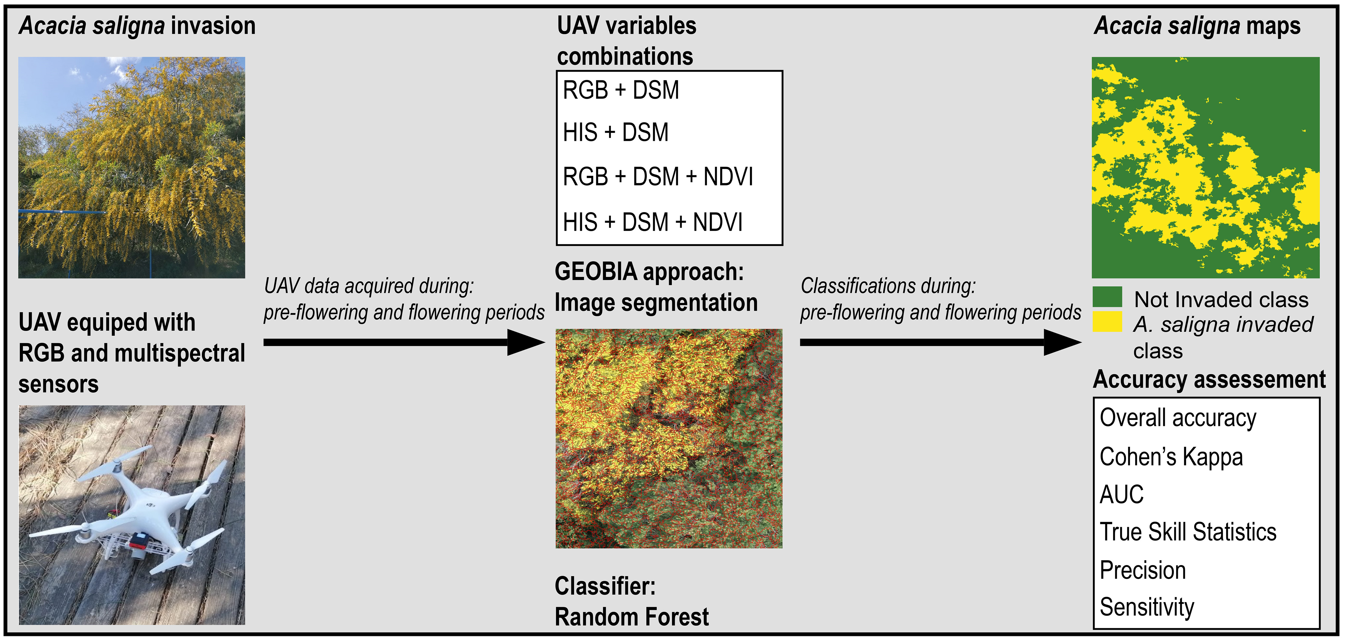
2. Materials and Methods

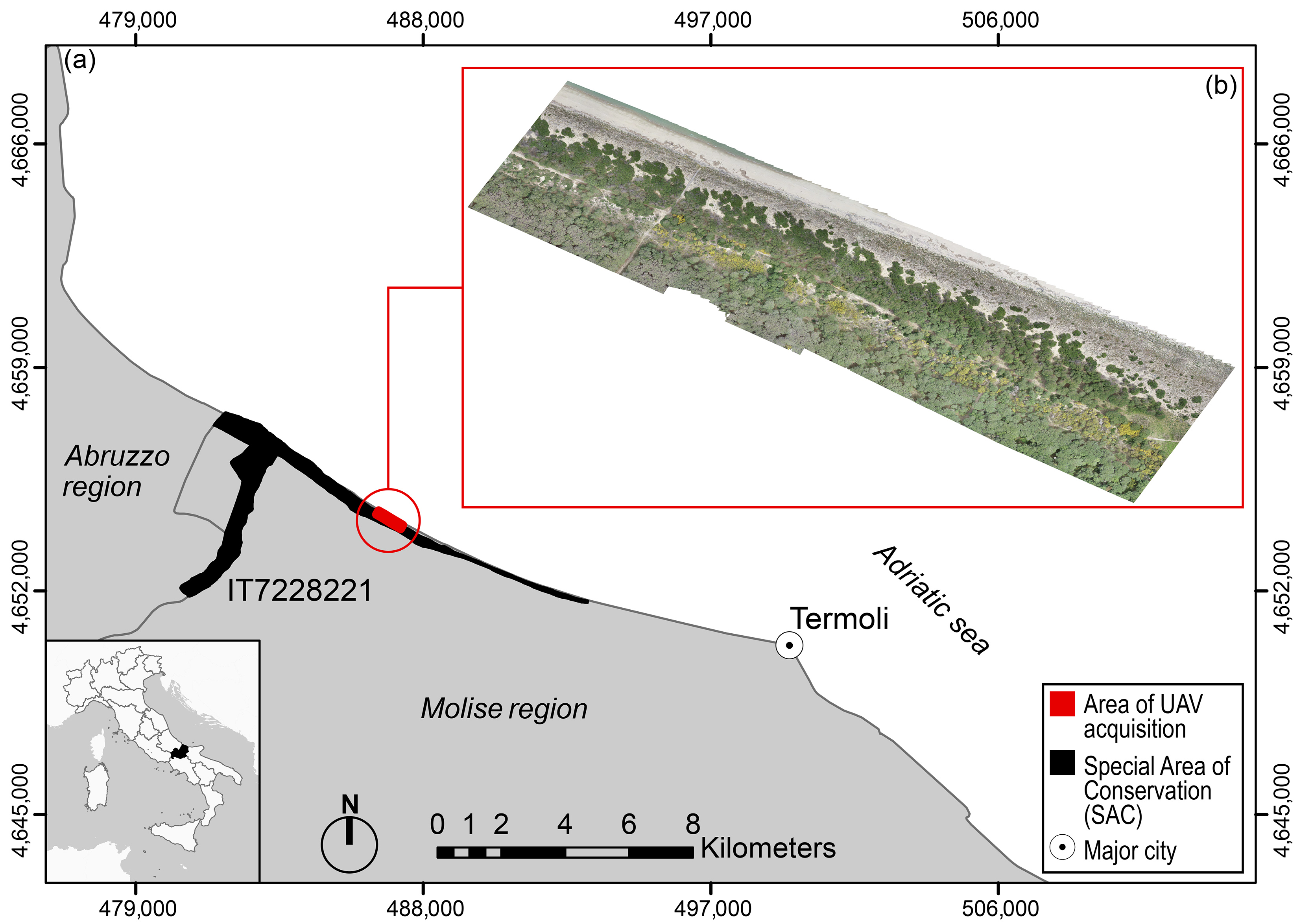
2.1. Study Area and Target Species

The study area includes a tract of Mediterranean coastal dunes located on the Adriatic coast of Central Italy (Molise region; Figure 1). It consists of approximately 11 ha of recent coastal dunes (Holocene) occupying a narrow strip parallel to the seashore [53,54] and is included in a Special Area of Conservation (SAC, Habitat Directive 92/43/EEC; Foce Trigno–Marina di Petacciato IT7228221) and it is part of a Long—Term Ecological Research site [55,56]. The presence within the study area of a Long—Term Ecological Research site (LTER, http://www.lter-europe.net/ (accessed on 21 August 2021)), gathering a valuable amount of long—term ecological data represents an excellent training ground to develop methodologies able to evaluate invasion processes at present and over time [57].

It hosts the typical sea–to–inland vegetation zonation ranging from pioneer annual communities on the seashore, followed by perennial herbaceous vegetation on mobile dunes, small chamaephytes communities intermingled with therophytic grasslands on embryonic dunes, evergreen shrubs and small sclerophyllous trees on fixed dunes and forests in foredunes [56,58,59]. The analyzed area is dominated by natural and semi–natural vegetation being artificial areas and cropland absent (Figure 1). In this area, A. saligna was planted during the 50s along a narrow strip between wooded dunes and fixed dunes, for sand stabilization and for sheltering foredune forests and agricultural areas from winds and salt spray [40,42,60].

2.2. Data Collection and Analysis

Data collection and analysis were performed according to the following steps: (a) UAV image acquisition and orthomosaicking, (b) image pre—processing and variables calculation, (c) Object—Based Image Analysis and classification, and (d) accuracy assessment (Figure 2). The procedure was implemented separately for remote sensed data collected in pre-flowering and in flowering periods.

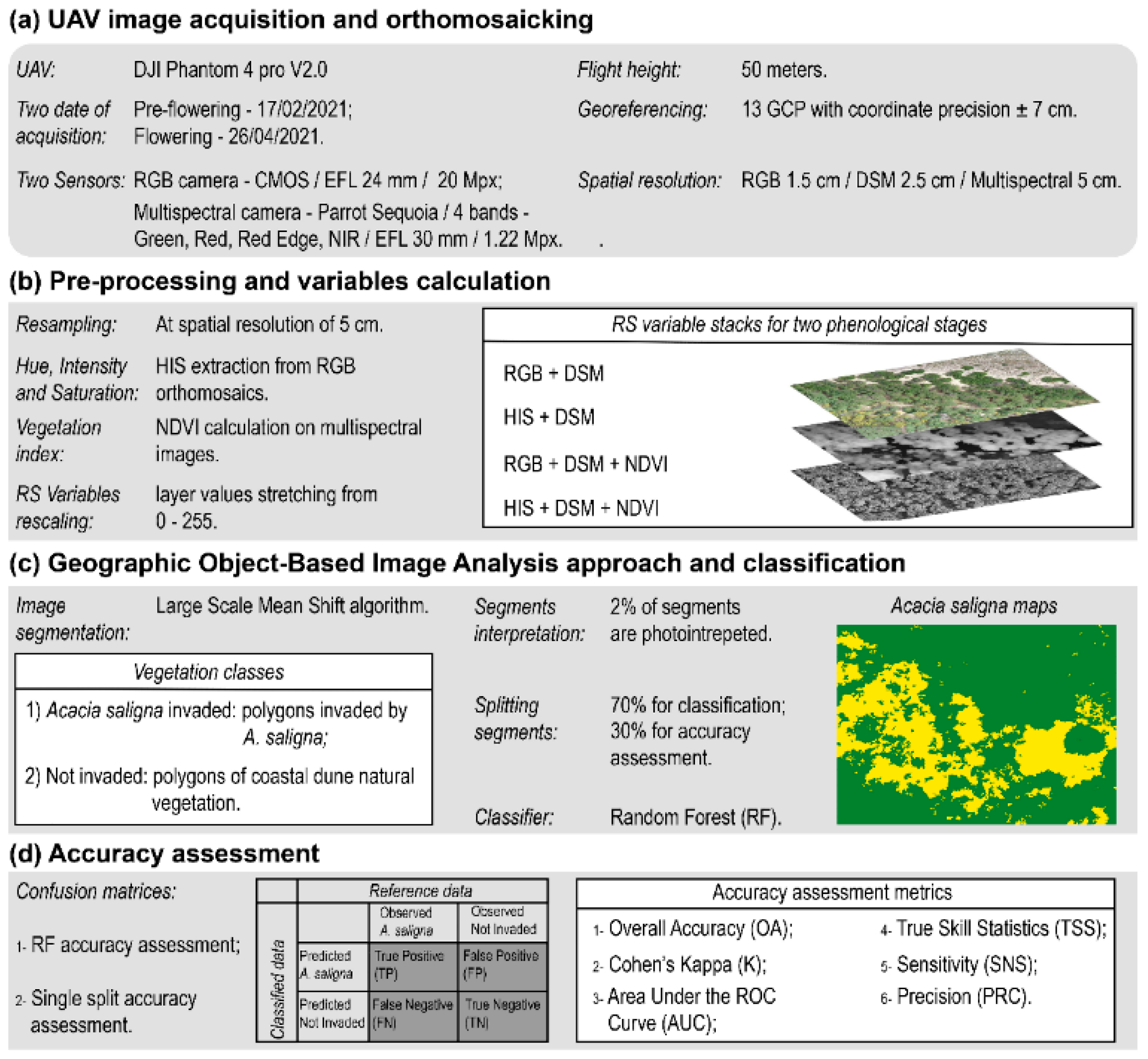
2.2.1. UAV Image Acquisition and Orthomosaicking

A multirotor quadcopter DJI Phantom 4 Pro V2.0 was used to collect the aerial images during A. saligna pre-flowering (17 February 2021) and flowering periods (26 April 2021, Figure 2). This UAV is equipped with the CMOS (Complementary Metal Oxide Semiconductor) sensor, a Red–Green–Blue (RGB) camera with 20 Mpx and 24 mm of Equivalent Focal Lengt (EFL), and in addition, we equipped the UAV with the Parrot Sequoia multispectral camera with four bands, each with 1.2 Mpx and EFL of 30 mm: Green (G, bandwidth: 550 nm ± 40 nm); Red (R, bandwidth: 660 nm ± 40 nm), Red Edge (RE, bandwidth: 735 nm ± 10 nm), and Near Infrared (NIR, bandwidth: 790 nm ± 40 nm).

The freeware mobile application Pix4Dcapture (version 4.11.0 for Android, https://www.pix4d.com/product/pix4dcapture (accessed on 21 August 2021)) was used for flight planning. To obtain standardized data, we used the same settings for all flights performed. The flights’ altitude was set at 50 m relatively to the take-off point, at a 5 m/s speed; all the flights were made between 10:00 a.m. and 12:00 a.m.. Finally, the images overlap was set to 80% for both forward and side overlaps. For the setting of the Parrot Sequoia camera, we used the dedicated HTML interface, accessible by connecting the camera to the smartphone via Wi–Fi. We have entered the same flight altitude and image overlap values as previously described (for Pix4Dcapture application) within the HTML interface. The two sensors captured images simultaneously during the flights; the CMOS sensor is trigged by Pix4Dcapture, while Parrot Sequoia camera by HTML interface.

Before the flights, we positioned 12 Ground Control Point (GCPs) target of 50 cm² over the flight area. GCPs coordinates (longitude, latitude, and altitude) were measured using a high accuracy GNSS receiver (Trimble R2) connected to the HxGN SmartNet GNSS positioning services for RTK (nearest) correction with nominal and estimated horizontal accuracies of 1 and 7 cm respectively.

All aerial images were processed using a Structure for Motion approach (SfM) by Agisoft Metashape Professional (version 1.6.2, https://www.agisoft.com/ (accessed on 21 August 2021)). We produced, for each flight, the RGB orthomosaic and Digital Surface Model (DSM) using the aerial images derived by RGB sensor, and the orthomosaics of G, R, RE, and NIR bands by aerial images of multispectral sensor. We georeferenced these data by the coordinates of GCPs [61,62]. The spatial resolutions of the pre-flowering and flowering periods were of 1.5 cm in the RGB orthomosaics, of 2.5 cm in DSMs, and of 5 cm in the four multispectral bands.

2.2.2. Pre-Processing and Variables Extraction

First, we resampled the RGB orthomosaic and the DSM to the coarser spatial resolution of multispectral images (5 cm) using a bilinear resampling algorithm [63]. In order to improve the spectral resolution of the RGB images we considered Hue, Intensity and Saturation metrics (HIS) [64,65,66] using the i.rgb.his tool implemented in GRASS GIS 7.8 [67]. As hue refers to the dominant wavelength of light inside the pixel, intensity refers to the total brightness of a colour measured as the relative degree of black or white, and saturation refers to the purity of the colour defined as the absence of mixture in a completely saturated pixel with no other frequencies [68,69,70].

Then, we derived from the multispectral orthomosaic the Normalized Difference Vegetation index (NDVI) as follows Equation (1) [71]:

$$\mathrm{NDVI}=\frac{NIR-R}{NIR+R}$$

(1)

This vegetation index is widely considered as a proxy of photosynthetic biomass and productivity and it has been successfully used for IAPs mapping [19]. Since the remote sensed variables have different units of measurement and thus would potentially affect the classification results, we standardised the bands values from 0 to 255 [72,73]. Lastly, we created for image classification a set of stacks including the following combinations of variables: (i) DSM + RGB (ii) DSM + HIS; (iii) DSM + RGB + NDVI and (iv) DSM + HIS + NDVI. The pre—processing procedures were applied to the images acquired in the pre-flowering and flowering periods separately, building four raster stacks in pre-flowering period and four raster stacks in the flowering period (eight raster stacks) for classification.

2.2.3. Geographic Object—Based Image Analysis and Classification

To detect and map A. saligna invaded areas and natural vegetation along the analysed coastal landscape we adopted a Geographic Object—Based Image Analysis approach (GEOBIA) [74,75,76], followed by Random Forest classification procedure that was repeated for each of the 8 RS variables stacks built in the previous step. GEOBIA consists of image segmentation based on the raster stack information. These segments are the basic units for classification, and they consist in homogeneous regions [75,77,78].

Image segmentation was performed using the Large Scale Mean Shift (LSMS) algorithm implemented in the open–source software Orfeo Toolbox [79,80]. The LSMS is a non–parametric and iterative clustering algorithm grouping image regions by spatial and spectral closeness into homogenous segments [78,81]. For implementing LSMS we fixed three parameters: Spatial Radius (sr) defined the maximum spatial Euclidean distance between pixels to cluster in the same polygon; Range Radius (rr), the maximum Euclidean spectral distance between pixels to cluster in the same polygon; Minimum Segment Size (ms) the minimum number of pixels per segment to define a polygon. We adopted different combinations of these parameters by tuning them at 5 steps intervals and after an accurate visual inspection we chose the following combination: sr = 5 m., rr = 5 m. and ms = 100 pixels.

Then, for each segmented image we selected 2915 random segments (which correspond to the ~2% of the total segments) and we classified them by visual interpretation of RGB orthomosaics in A. saligna invaded class (305 polygons) and not invaded vegetation class (2610 polygons). We used a threshold rule of 50% cover for the determination of classes. The random selection of segments ensures a representative sample of classes occurring in the landscape [82]. These segments (invaded and not invaded) were split in two datasets (including the 70% and the 30% of segments) following a random stratified sampling approach and used for training and for testing procedures (accuracy assessment) [83,84,85].

Classification and mapping of A. saligna (using the pre-flowering or flowering images) were performed using random forest (RF) which is an ensemble machine learning algorithm that operates by constructing a large number of decision trees to generate classifications and spatial predictions [86,87,88] and that is particularly effective for RS supervised classification [89,90,91]. RF classification parameters were selected by running on the training data 10-fold cross validation series using the “caret” R package (function train) [92]. In particular for each segmented image we tune up different parameters and selected their best combination based on cross—validation procedures [93]. RF required two parameters: the number of uncorrelated decision trees (Ntree) and the number of variables randomly selected at each node of decision trees (Mtry) [94]. Specifically, to optimize RF parameters we set a high number of uncorrelated decision trees (Ntree = 1000), while we tested different combinations of Mtry parameter, with values ranging from 2 to the total number of variables, and split rules, then we chose the combination that yielded the highest accuracy value [24,59].

Finally, we estimated the relative importance of variables on classification using two indices the Mean Decrease Accuracy (MDA) and Mean Decrease Gini (MDG) [95]. The MDA index quantifies the importance of a variable repeating the classification after its random exclusion. Greater the difference between results in percentage, greater the importance of variable. The MDG is a measure of how each variable contributes to the homogeneity of the nodes in the resulting of RF [96,97]. Thus, higher the values of MDA and MDG, higher the importance of the variables in the classification.

2.2.4. Accuracy Assessment

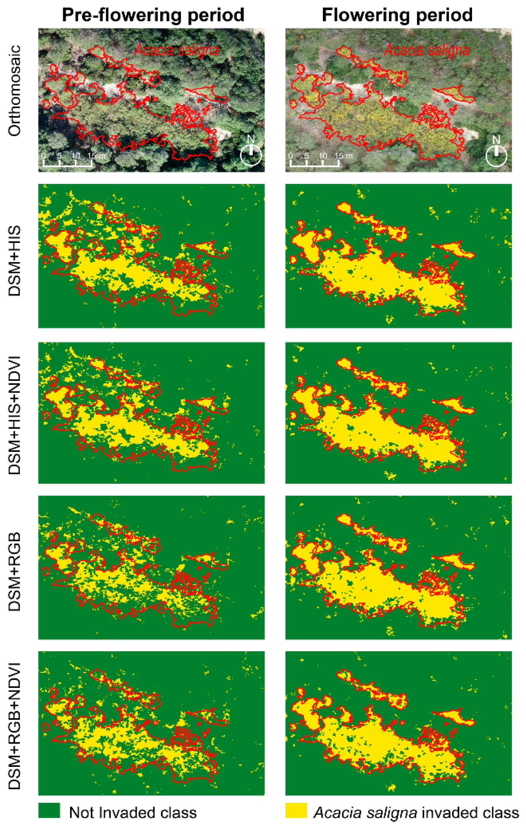
We calculated the accuracy of the obtained maps by two types of confusion matrices, the first derived from the internal 10-fold cross validation of RF (RF accuracy assessment) [82,87] and the second based on the photointerpretation of test polygons (30% of the polygons, single split accuracy assessment) [98,99]. We computed the following performance metrics: the Overall Accuracy (OA), the Cohen’s Kappa (K), the Area Under the ROC Curve (AUC), True Skill Statistics (TSS), and Sensitivity (SNS) and Precision (PRC,

Table 1. Accuracy assessment metrics selected for comparing the performance of classifications using two confusion matrices types, the internal confusion matrix of RF and an independent confusion matrix derived by photointerpretation of polygons test. N, total number of testing data; TP, True Positive; FP, False Positive; TN, True Negative; FN, False Negative (see Figure 2).

Acronym	Name	Formula
OA	Overall Accuracy	$\frac{\mathrm{TP}+\mathrm{TN}}{\mathrm{TP}+\mathrm{FN}+\mathrm{TN}+\mathrm{FP}}$
K	Cohen’s Kappa	$\frac{\mathrm{OA}-\frac{1}{{\mathrm{N}}^2}[\left(\mathrm{TP}+\mathrm{FN}\right)*\left(\mathrm{TP}+\mathrm{FP}\right)+\left(\mathrm{FP}+\mathrm{TN}\right)*\left(\mathrm{FN}+\mathrm{TN}\right)]}{1-\frac{1}{{\mathrm{N}}^2}[\left(\mathrm{TP}+\mathrm{FN}\right)*\left(\mathrm{TP}+\mathrm{FP}\right)+\left(\mathrm{FP}+\mathrm{TN}\right)*\left(\mathrm{FN}+\mathrm{TN}\right)]}$
AUC	Area Under the ROC Curve	$\frac{1}{2}\left(\frac{\mathrm{TP}}{\mathrm{TP}+\mathrm{FN}}+\frac{\mathrm{TN}}{\mathrm{TN}+\mathrm{FP}}\right)$
TSS	True Skill Statistics	$\frac{\mathrm{TP}}{\mathrm{TP}+\mathrm{FN}}+\frac{\mathrm{TN}}{\mathrm{TN}+\mathrm{FP}}-1$
SNS	Sensitivity	$\frac{\mathrm{TP}}{\mathrm{TP}+\mathrm{FN}}$
PRC	Precision	$\frac{\mathrm{TP}}{\mathrm{TP}+\mathrm{FP}}$

) also known as producer’s and user’s accuracy, respectively [100]. The OA is a measure of overall effectiveness of a classification, its values range from 0%, total absence of accuracy in classification to 100%, a perfect classification. OA values greater than 85% are considered as acceptable results [101]. The Cohen’s Kappa metrics measures the agreement between predicted and observed polygons and it reveals the degree of reliability of classification [101]. K values range from 0 (no predictive ability) to 1 (perfect predictive ability), and Landis & Koch [102] suggest the following ranges: K ≥ 0.80 almost perfect reliability, 0.60 ≤ K < 0.80 substantial reliability, 0.40 ≤ K < 0.60 moderate reliability, 0.20 ≤ K < 0.40 fair reliability, and K ≤ 0.20 slight or poor reliability. An alternative measure is the Area Under the ROC Curve (AUC) defining the ability of classification to separate A. saligna polygons from the Not Invaded polygons. The AUC is the probability that a randomly selected A. saligna polygon will outscore a randomly drawn Not Invaded plot, and classification with AUC values equal or higher 0.7 are considered with good capacity of separability, while AUC ≥0.90 identified classification with excellent capacity of separability [103,104]. The TSS is another accuracy metric comparing the number of correct forecasts, minus those attributable to random guessing, to that of a hypothetical set of perfect forecasts [105]. The TSS range varies from −1 to 1, where 1 indicates perfect agreement and values equal or lesser of 0 indicate random classification [105]. The SNS estimates the effectiveness of classification to identify the A. saligna polygons, its values range from 0%, no effectiveness to identify A. saligna, to 100%, perfect effectiveness to identify A. saligna [106]. The PRC evaluates the correctness of classification and it represents the probability of A. saligna polygons observed are predicted by classification. PRC ranges from 0%, the A. saligna polygons observed are not predicted, to 100% perfect correctness of classification [107]. It is important to note that most of these metrics has some limitations that should be considered for their accurate interpretation. For example, both OA and AUC are highly sensitive to imbalanced data [108], whereas SNS, PRC, TSS and K are less sensitive [109].

Accuracy metrics were used to compare the performance of the classification derived from pre-flowering and flowering images and the potential of the different combinations of RS variables (eight classifications: four combinations of variables for classifying images acquired in the two time periods).

3. Results

All the performed classifications mapped the A. saligna with acceptable accuracy values with OA and AUC values always higher than 90% and 0.77 respectively (Figure 3,

Table 2. Accuracy assessment (AA) values of the classifications obtained using the 4 different RS UAV stacks of variables derived from images collected during pre-flowering and flowering periods. Accuracy values calculated by internal 10-fold cross validation of Random Forest (RF ± Standard deviation) and by an independent independent single split (SS) are reported. Overall accuracy (OA) in percentage, Kappa statics (Kappa), Area Under of the ROC Curve (AUC), True Skill Statistics (TSS), Sensitivity (SNS), and Precision (PRC) in percentage.

Pre—Flowering Period
Raster Stack	AA	OA (%)	K	AUC	TSS	SNS (%)	PRC (%)
DSM + HIS	RF	93.37 ± 0.67	0.57 ± 0.06	0.90 ± 0.02	0.48 ± 0.09	52.49 ± 8.82	76.55 ± 6.64
	SS	93.61	0.62	0.77	0.54	56.18	78.12
DSM + RGB	RF	91.17 ± 0.80	0.38 ± 0.07	0.84 ± 0.01	0.30 ± 0.09	31.09 ± 8.58	65.42 ± 7.57
	SS	94.42	0.66	0.80	0.60	61.45	78.46
DSM + HIS + NDVI	RF	93.05 ± 1.06	0.55 ± 0.11	0.90 ± 0.02	0.47 ± 0.12	49.01 ± 11.71	74.04 ± 6.35
	SS	94.33	0.65	0.79	0.58	60	78.13
DSM + RGB + NDVI	RF	91.20 ± 0.79	0.39 ± 0.07	0.87 ± 0.02	0.31 ± 0.09	30.96 ± 9.37	69.02 ± 11.21
	SS	94.28	0.68	0.82	0.64	66.67	76.32
Flowering Period
Raster Stack	AA	OA (%)	K	AUC	TSS	SNS (%)	PRC (%)
DSM + HIS	RF	94.92 ± 0.60	0.73 ± 0.04	0.95 ± 0.01	0.65 ± 0.07	65.77 ± 8.27	88.73 ± 4.33
	SS	96.61	0.82	0.88	0.75	75.76	94.94
DSM + RGB	RF	93.35 ± 0.49	0.62 ± 0.04	0.91 ± 0.01	0.51 ± 0.05	51.51 ± 5.19	88.57 ± 4.52
	SS	95.60	0.76	0.83	0.66	66.67	95.65
DSM + HIS + NDVI	RF	94.92 ± 0.92	0.75 ± 0.05	0.95 ± 0.01	0.67 ± 0.08	67.95 ± 8.70	88.96 ± 5.42
	SS	95.75	0.80	0.87	0.74	74.75	94.94
DSM + RGB + NDVI	RF	92.56 ± 1.21	0.61 ± 0.08	0.91 ± 0.02	0.51 ± 0.10	51.29 ± 10.16	89.36 ± 10.76
	SS	95.87	0.80	0.86	0.72	72.45	94.67

). However, only in the flowering period the polygons of A. saligna are very well identified as evinced by the increase of K, TSS, PRC and SNS values compared by pre-flowering period (Figure 3, Table 2).

Considering the Pre—Flowering period, the RF accuracy assessment indicated the DSM + HIS as the best combination of variables (Table 2), with high values of overall accuracy (OA: 93.37 ± 0.67%) and capacity of separability (AUC: 0.90 ± 0.02), a moderate reliability (K: 0.57 ± 0.06), an intermediate agreement (TSS: 0.48 ± 0.09) and a significant correctness of classification to identify A. saligna (PRC: 76.55 ± 6.64%) with a sensitivity of classification (SNS: 52.49 ± 8.82%). According with the single split accuracy assessment, the best combination of variables for classifying of pre-flowering images are DSM + RGB assessed with OA and PRC procedures, and DSM + RGB + NDVI considering K, AUC, TSS and SNS (Table 2).

A. saligna classification obtained from the flowering period images presented excellent accuracy values using DSM + HIS + NDVI and DSM + HIS with highest values for single split accuracy assessment (Table 2). In the RF accuracy assessment, these two classifications diverged slightly by K, TSS, Precision and Sensitivity with higher values obtained by the DSM + HIS + NDVI classification. However, the DSM + RGB + NDVI evidenced the best effectiveness in correctness of classification reaching PRC around 90% according the internal accuracy of RF (Table 2). In the single split accuracy assessment, the DSM + HIS classification showed slight divergences with highest values in all accuracy assessment metrics except for PRC compared to DSM + HIS + NDVI (equal value) and DSM + RGB (higher value, Table 2).

The contribution of RS variables for A saligna mapping included in the different stacks, widely varied among the pre-flowering or flowering UAV images classifications, with the exception of Hue and Red which resulted always important (Figure 4, Supplementary Materials Figure S1). DSM is relevant on classifications based on pre–flowering images and assumes a secondary role on flowering images (Figure 4, Supplementary Materials Figure S1). Saturation values of A. saligna patches and Not Invaded areas during the flowering period are significantly different, assuming an important role for image classification (Figure 4). Also, Blue variable resulted important in flowering image classification, still it assumes comparable values on the mapped classes (Figure 4).

Concerning A saligna maps based on pre-flowering UAV images, Hue resulted the most important variable on classifications using HIS (e.g., DSM + HIS and DSM + HIS + NDVI stacks; Figure 4), followed by the DSM (e.g., high MDA and MDG values). The inclusion of NDVI variable had a limited effect and low importance on the obtained classification (e.g., NDVI assumed similar values on both classes; Supplementary Materials Figure S1). In the classifications supported by RS stacks including RGB (e.g., DSM + RGB and DSM + RGB + NDVI; Table 2), the DSM resulted the most important variable, followed by the Red band with NDVI assuming a less important role (Figure 4).

On A. saligna maps based on UAV images registered during the flowering period, the most important variables were Saturation and the Hue, followed by DSM being the NDVI the less important variable. In maps using RGB (e.g., DSM + RGB and DSM + RGB + NDVI; Table 2), the most important variables are the Red assuming significant different values on the mapped classes and the Blue bands, which instead assumes similar values (Figure 4, Supplementary Materials Figure S1).

4. Discussion

In this paper, we tested the potential of fine-scale UAV data collected during pre-flowering and flowering periods to detect and map A. saligna on Mediterranean coastal dunes.

UAV images, derived by RGB and multispectral sensors allowed to produce very accurate maps of A. saligna distribution growing on coastal dunes. UAV image classification resulted an efficient method for mapping of IAPs, also in complex environments offering a sound support to the prioritization of conservation and management actions claimed by the EU IAS Regulation 1143/2014. Notice that the obtained classification effectively identified and mapped almost all the invaded areas even those occurring on very small patches hardly detectable using coarser RS data as airborne or satellite images [29,110]. Such results confirmed the importance of UAVs for detection and mapping of IAPs [32,111]. A. saligna resulted very effectively mapped by UAV images captured on flowering periods, with map accuracy reaching very high values. Specifically, the classification derived by HIS variables (DSM + HIS, DSM + HIS + NDVI) resulted particularly appropriate for mapping A. saligna, supporting excellent accuracy values, and assuring the detection of almost all the A. saligna patches. The accuracy of A. saligna maps derived from pre-flowering images resulted acceptable but with lower values compared with classifications based on flowering UAV images.

We observed a slight difference in the overall effectiveness and the ability of classification expressed by OA and AUC, on maps derived from pre-flowering and flowering images which is likely influenced by the not invaded class which spectral characteristics remain similar between the two periods. In addition, it has been demonstrated that overall accuracy and AUC should not be considered as the only metrics to assess the goodness of map classification since it does not reflect error distribution among categories and its value is greatly influenced by the dominant category, category as in the case of imbalanced data [112,113], which in our case is the Not Invaded class. On the contrary, K, TSS, SNS and PRC provide more robust results in the case of imbalanced data [109].

As observed for other Acacia species [43,49,114], also in our case, the huge number of yellow flowers allowed to effectively distinguish the IAP from the native vegetation background and soil features (e.g., very high values of K and TSS overall accuracy and high SNS and PRC for A. saligna class). As can be seen in Figure 3, the results of the classifications during the flowering period shows a similar extent of invasion of A. saligna, with large and compact patches. On the contrary, the classifications in the pre-flowering period resulted in less compact and fragmentated patches (low values of K, TSS and SNS).

This distinctive phenological characteristic is well captured by the HIS variables and in particular by Hue and Saturation, whereas the maps based on RGB variables showed moderate values of SNS (<60%), demonstrating their lower effectiveness for A. saligna classification (Figure 5). The yellow color of A. saligna flowers assume very high values of Saturation or purity of color and very low values of Hue or dominant color (Figure 5, Supplementary Materials Figure S1). During the blooming peak, Acacia flowers assume an almost pure yellow color, which make them distinguishable from the background (Figure 5) [115,116].

Notice that on costal dunes also some native herbaceous species have yellow flowers (e.g., Medicago marina, Lotus cytisoides, Ononis variegata) in a similar blooming period. Still, unlike the analyzed IAP, these native species present low cover and occur on the herbaceous layer, characteristic easily detected by DSM [110,117]. Furthermore, DSM assumed a considerable importance on the classification of pre-flowering images, depicting the differences in height and canopy of A. saligna and dune natural vegetation [118]. However, all classifications slightly distinguished the A. saligna polygons in the pre-flowering period, as evinced by low values of K, TSS, PRC and in particular of SNS. These low values could be due either to large variability of coloration in the leaves of A. saligna and/or RGB values similar to native coastal dune vegetation in particular woody and scrubs vegetation.

The inclusion of NDVI in the variables stack for classification of pre-flowering and flowering images does not improve map accuracy. As observed for other invasion processes (e.g., Phragmites australis, Fallopia japonica) NDVI plays a secondary role on A. saligna mapping which is even weaker on classifications based on blooming UAV images [110,119].

Such results are particularly important as using a simple RGB sensor mounted on an UAV reduces costs and computational efforts [24,120,121] allowing to optimize time and economic commitment necessary for detecting and mapping invasive species in complex environments as coastal dunes. In the light of our findings, we can affirm that UAV images taken with a RGB sensor and converts with HIS variables during the blooming period could represent a sound support for IAPs detection and mapping also in complex and dynamic environments, supporting the prioritization of the concrete actions claimed by the EU IAS Regulation 1143/2014 [43,122].

Data collection and classification approach adopted in this study are easily repeatable and can be extended to map invaded coastal areas by A. saligna on other regions and environmental conditions. In this context, UAV images are good candidates for becoming a fundamental instrument for IAPs detection as well as for monitoring their invasion status over time [29,30,122,123].

Notice that the multirotor quadcopter used in this study limited the spatial extension of the obtained multispectral images. On the other hand, the higher autonomy of fixed wing UAV acquiring RGB images allowed to cover wider areas [110,122,124] which in addition to the great effectiveness of DSM and HIS variables support this sensor as the best candidate for A. saligna mapping and monitoring on coastal areas.

5. Conclusions

In this work, we used an approach based on UAV data to detect and map A saligna invasion on a dynamic and heterogeneous coastal dunes landscape. Actually, mapping IAPs on these ecosystems can be a major challenge and cannot rely only on satellite images due to some limitations (e.g., course spatial resolution, high cost, errors in georeferencing). For example, the existing freely available RS data (e.g., Landsat, Sentinel, or Planet Scope) have high—medium spatial resolution which are not often suitable for depicting the fine—grain of coastal landscape mosaic, while higher spectral resolution data can attain higher costs (e.g., World View, Quick Bird, IKONOS, Pléiades, or LiDAR). In addition, the accurate detection of invasive species requires data with very high temporal resolution to capture the different phenological phases that would help to distinguish such species from the natural vegetation. In our work, we have demonstrated that the timing of data collection is crucial for mapping A. saligna since the inflorescence, which remain yellow only for few weeks, effectively helped to classify the species.

The proposed UAV approach is cost–effective and suited for providing high spatial and temporal resolution data for IAPs detection and mapping on coastal landscapes; however, due to technical constraints of the UAV technology (i.e., capability of batteries, surveying restrictions) it is eligible only for mapping relatively small areas. Further efforts should be devoted to harmonizing UAV ultra-high spatial resolution data covering small extents with RS medium—high spatial resolution data but covering wider areas. An effort on identifying adequate upscaling procedures able to extrapolate similar information from local to regional and national scales are needed. The proposed GEOBIA approach for IAPs detection and mapping on coastal dunes could help to define improved protocol for IAPs monitoring and for prioritizing conservation actions in these dynamic and highly vulnerable landscapes.

Our results evidenced the great potential of UAV images and in particular the transformation of RGB images to the HIS model, for producing accurate maps of A. saligna also in complex and dynamic coastal dunes landscapes, offering a sound support to the prioritization of conservation and management actions claimed by the EU IAS Regulation 1143/2014. The utilization of innovative RS data on LTER sites offers further insights for improving monitoring efforts, thus optimizing the resources and time devoted to managing IAPs. The extension of the proposed approach to the wider LTER observation network could be a good opportunity to provide a monitoring tool in these areas with low spatial extensions but with high conservation value.

References

1. Hulme, P.E. Trade, transport and trouble: Managing invasive species pathways in an era of globalization. J. Appl. Ecol. 2009, 46, 10–18. [Google Scholar] [CrossRef]
2. Pyšek, P.; Richardson, D.M. Invasive species, environmental change and management, and health. Annu. Rev. Environ. Resour. 2010, 35, 25–55. [Google Scholar] [CrossRef] [Green Version]
3. Simberloff, D.; Martin, J.L.; Genovesi, P.; Maris, V.; Wardle, D.A.; Aronson, J.; Courchamp, F.; Galil, B.; García-Berthou, E.; Pascal, M.; et al. Impacts of biological invasions: What’s what and the way forward. Trends Ecol. Evol. 2013, 28, 58–66. [Google Scholar] [CrossRef] [Green Version]
4. Pyšek, P.; Hulme, P.E.; Simberloff, D.; Bacher, S.; Balckburn, T.M.; Carlton, J.T.; Dawson, W.; Essl, F.; Foxcroft, L.C.; Genovesi, P.; et al. Scientists’ warning on invasive alien species. Biol. Rev. 2020, 95, 1511–1534. [Google Scholar] [CrossRef]
5. Lazzaro, L.; Bolpagni, R.; Buffa, G.; Gentili, R.; Lonati, M.; Stinca, A.; Acosta, A.T.R.; Adorni, M.; Aleffi, M.; Allegrezza, M.; et al. Impact of invasive alien plants on native plant communities and Natura 2000 habitats: State of the art, gap analysis and perspectives in Italy. J. Environ. Manag. 2020, 274, 111140. [Google Scholar] [CrossRef]
6. Bartz, R.; Kowarik, I. Assessing the environmental impacts of invasive alien plants: A review of assessment approaches. NeoBiota 2019, 43, 69–99. [Google Scholar] [CrossRef] [Green Version]
7. Jucker, T.; Carboni, M.; Acosta, A.T.R. Going beyond taxonomic diversity: Deconstructing biodiversity patterns reveals the true cost of iceplant invasion. Divers. Distrib. 2013, 19, 1566–1577. [Google Scholar] [CrossRef]
8. Blackburn, T.M.; Essl, F.; Evans, T.; Hulme, P.E.; Jeschke, J.M.; Kühn, I.; Kumschick, S.; Marková, Z.; Mrugała, A.; Nentwig, W.; et al. A unified classification of alien species based on the magnitude of their environmental impacts. PLoS Biol. 2014, 12, e1001850. [Google Scholar] [CrossRef] [PubMed] [Green Version]
9. Loiola, P.P.; de Bello, F.; Chytrý, M.; Götzenberger, L.; Carmona, C.P.; Pyšek, P.; Lososová, Z. Invaders among locals: Alien species decrease phylogenetic and functional diversity while increasing dissimilarity among native community members. J. Ecol. 2018, 106, 2230–2241. [Google Scholar] [CrossRef]
10. Tordoni, E.; Petruzzellis, F.; Nardini, A.; Savi, T.; Bacaro, G. Make it simpler: Alien species decrease functional diversity of coastal plant communities. J. Veg. Sci. 2019, 30, 498–509. [Google Scholar] [CrossRef]
11. Gutiérrez, J.L. Modification of Habitat Quality by Non-native Species. In Impact of Biological Invasions on Ecosystem Services, 1st ed.; Vilà, M., Hulme, P., Eds.; Invading Nature-Springer Series in Invasion Ecology: Cham, Switzerland, 2017; Volume 12, pp. 33–47. [Google Scholar]
12. Bonari, G.; Fantinato, E.; Lazzaro, L.; Sperandii, M.G.; Acosta, A.T.R.; Allegrezza, M.; Assini, S.; Caccianiga, M.; Di Cecco, V.; Frattaroli, A.; et al. Shedding light on typical species: Implications for habitat monitoring. Plant Sociol. 2021, 58, 157–166. [Google Scholar] [CrossRef]
13. Rai, P.K.; Singh, J.S. Invasive alien plant species: Their impact on environment, ecosystem services and human health. Ecol. Indic. 2020, 111, 106020. [Google Scholar] [CrossRef]
14. Jones, B.A. Tree shade, temperature, and human health: Evidence from invasive species-induced deforestation. Ecol. Econ. 2019, 156, 12–13. [Google Scholar] [CrossRef]
15. European Commission. Invasive Alien Species. A European Response, 1st ed.; European Union: Brussels, Belgium, 2014; pp. 1–28. [Google Scholar]
16. Branquart, E.; Brundu, G.; Buholzer, S.; Chapman, D.; Ehret, P.; Fried, G.; Starfinger, U.; van Valkenburg, J.; Tanner, R. A prioritization process for invasive alien plant species incorporating the requirements of EU Regulation no. 1143/2014. Bull. OEPP/EPPO Bull. 2016, 46, 603–617. [Google Scholar] [CrossRef] [Green Version]
17. Sitzia, T.; Campagnaro, T.; Kowarik, I.; Trentanovi, G. Using forest management to control invasive alien species: Helping implement the new European regulation on invasive alien species. Biol. Invasions 2016, 18, 1–7. [Google Scholar] [CrossRef]
18. Lozano, V.; Marzialetti, F.; Carranza, M.L.; Chapman, D.; Branquart, E.; Dološ, K.; Große-Stoltenberg, A.; Fiori, M.; Capece, P.; Brundu, G. Modelling Acacia saligna invasion in a large Mediterranean island using PAB factors: A tool for implementing the European legislation on invasive species. Ecol. Indic. 2020, 116, 106516. [Google Scholar] [CrossRef]
19. Vaz, A.S.; Alcaraz-Segura, D.; Campos, J.C.; Vicente, J.R.; Honrado, J.P. Managing plant invasions through the lens of remote sensing: A review of progress and the way forward. Sci. Total Environ. 2018, 642, 1328–1339. [Google Scholar] [CrossRef]
20. Müllerová, J.; Pergl, J.; Pyšek, P. Remote sensing as a tool for monitoring plant invasions: Testing the effects of data resolution and image classification approach on the detection of a model plant species Heracleum mantegazzianum (giant hogweed). Int. J. Appl. Earth Obs. 2013, 25, 55–65. [Google Scholar] [CrossRef]
21. Niphadkar, M.; Nagendra, H. Remote sensing of invasive plants: Incorporating functional traits into the picture. Int. J. Remote Sens. 2016, 37, 3074–3085. [Google Scholar] [CrossRef]
22. Royimani, L.; Mutanga, O.; Odindi, J.; Dube, T.; Matongera, T.N. Advancements in satellite remote sensing for mapping and monitoring of alien invasive plant species (AIPs). Phys. Chem. Earth 2019, 112, 237–245. [Google Scholar] [CrossRef]
23. Peerbhay, K.; Mutanga, O.; Ismail, R. The identification and remote detection of alien invasive plants in commercial forests: An overview. S. Afr. J. Geomat. 2016, 5, 49–67. [Google Scholar] [CrossRef] [Green Version]
24. Kattenborn, T.; Lopatin, J.; Förster, M.; Braun, A.C.; Fassnacht, F.E. UAV data as alternative to field sampling to map woody invasive species based on combined Sentinel-1 and Sentinel-2 data. Remote Sens. Environ. 2019, 227, 61–73. [Google Scholar] [CrossRef]
25. Huang, C.; Asner, G.P. Applications of remote sensing to alien invasive plant studies. Sensors 2009, 9, 4869–4889. [Google Scholar] [CrossRef] [PubMed] [Green Version]
26. Bradley, B.A. Remote detection of invasive plants: A review of spectral, textural and phenological approaches. Biol. Invasions 2014, 16, 1411–1425. [Google Scholar] [CrossRef]
27. Pettorelli, N.; Laurance, W.F.; O’Brien, T.G.; Wegmann, M.; Nagendra, H.; Turner, W. Satellite remote sensing for applied ecologists: Opportunities and challenges. J. Appl. Ecol. 2014, 51, 839–848. [Google Scholar] [CrossRef]
28. Wang, X.; Wang, L.; Tian, J.; Shi, C. Object-based spectral-phenological features for mapping invasive Spartina alterniflora. Int. J. Appl. Earth Obs. 2021, 101, 102349. [Google Scholar] [CrossRef]
29. Nowak, M.M.; Dziób, K.; Bogawski, P. Unmanned aerial vehicles (UAVs) in environmental biology: A review. Eur. J. Ecol. 2018, 4, 56–74. [Google Scholar] [CrossRef]
30. Michez, A.; Piégay, H.; Jonathan, L.; Claessens, H.; Lejeune, P. Mapping of riparian invasive species with supervised classification of Unmanned Aerials System (UAS) imagery. Int. J. Appl. Earth Obs. 2016, 44, 88–94. [Google Scholar] [CrossRef]
31. Müllerová, J.; Brůna, J.; Bartaloš, T.; Dvořák, P.; Vítková, M.; Pyšek, P. Timing is important: Unmanned aircraft vs. satellite imagery in plant invasion monitoring. Front. Plant Sci. 2017, 8, 887. [Google Scholar] [CrossRef] [Green Version]
32. Bolch, E.A.; Santos, M.J.; Ade, C.; Khanna, S.; Basinger, N.T.; Reader, M.O.; Hestir, E.L. Remote detection of invasive alien species. In Remote Sensing of Plant Biodiversity, 1st ed.; Cavender-Bares, J., Gamon, J.A., Townsend, P.A., Eds.; Springer Nature: Cham, Switzerland, 2020; Volume 12, pp. 267–304. [Google Scholar]
33. Maslin, B.R. Studies in the genus Acacia-3. The taxonomy of A. salgina (Labill.) H. Wendl. Nuytsia 1974, 1, 332–340. [Google Scholar]
34. Thompson, G.D.; Bellstedt, D.U.; Richardson, D.M.; Wilson, J.R.U.; Le Roux, J.J. A tree well travelled: Global genetic structure of the invasive tree Acacia saligna. J. Biogeogr. 2015, 42, 305–314. [Google Scholar] [CrossRef]
35. Asefa, G.; Tamir, B. Effects of supplementing different forms of Acacia saligna leaves to grass hay on feed intake and growths of lambs. Trop Sci. 2006, 46, 205–208. [Google Scholar] [CrossRef]
36. George, N.; Henry, D.; Yan, G.; Byrne, M. Variability in feed quality between populations of Acacia saligna (Labill.) H. Wendl. (Mimosoideae)—Implications for domestication. Anim. Feed Sci. Technol. 2007, 136, 109–127. [Google Scholar] [CrossRef]
37. Avis, A.M. A review of coastal dune stabilization in the Cape province of South Africa. Landsc. Urban Plan. 1989, 18, 55–68. [Google Scholar] [CrossRef]
38. Bar, P.; Cohen, O.; Shoshany, M. Invasion rate of the alien species Acacia saligna within coastal sand dune habitats in Israel. Israel J. Plant Sci. 2004, 52, 115–124. [Google Scholar] [CrossRef]
39. Donaldson, J.E.; Hui, C.; Richardson, D.M.; Robertson, M.P.; Webber, B.L.; Wilson, J.R.H. Invasion trajectory of alien trees: The role of introduction pathway and planting history. Glob. Change Biol. 2014, 20, 1527–1537. [Google Scholar] [CrossRef]
40. Marzialetti, F.; Bazzichetto, M.; Giulio, S.; Acosta, A.T.R.; Stanisci, A.; Malavasi, M.; Carranza, M.L. Modelling Acacia saligna invasion on the Adriatic coastal landscape: An integrative approach using LTER data. Nat. Conserv. Bulg. 2019, 34, 127–144. [Google Scholar] [CrossRef]
41. Lehrer, D.; Becker, N.; Bar, P. The economic impact of the invasion of Acacia saligna in Israel. Int. J. Sustain. Dev. World Ecol. 2011, 18, 118–127. [Google Scholar] [CrossRef]
42. Del Vecchio, S.; Acosta, A.T.R.; Stanisci, A. The impact of Acacia saligna invasion on Italian coastal dune EC habitats. CR Biol. 2013, 336, 364–369. [Google Scholar] [CrossRef]
43. De Sá, N.C.; Castro, P.; Carvalho, S.; Marchante, E.; López-Núñez, F.A.; Marchante, H. Mapping the flowering of an invasive plant using Unmanned Aerial Vehicles: Is there potential for biocontrol monitoring? Front. Plant Sci. 2018, 9, 1–13. [Google Scholar] [CrossRef] [Green Version]
44. Paz-Kagan, T.; Silver, M.; Panov, N.; Karnieli, A. Multispectral approach for identifying invasive plant species based on flowering phenology characteristics. Remote Sens. 2019, 11, 953. [Google Scholar] [CrossRef] [Green Version]
45. Strydom, M.; Esler, K.J.; Wood, A.R. Acacia saligna seed banks: Sampling methods and dynamics, Western Cape, South Africa. S. Afr. J. Bot. 2012, 79, 140–147. [Google Scholar] [CrossRef]
46. Witkowski, E.T.F. Growth of seedlings of the invasive, Acacia saligna and Acacia Cyclops, in relation to soil phosphorus. Aust. J. Ecol. 1994, 19, 290–296. [Google Scholar] [CrossRef]
47. Gaol, M.L.; Fox, J.E.D. Reproductive potential of Acacia species in the central wheatbelt: Variation between years. Conserv. Sci. West. Aust. 2002, 4, 147–157. [Google Scholar]
48. Darcha, G.; Brhan, A.; Gebrewahid, Y.; Kassa, H.; Mezgebe, K.; Cunningham, P.; Hagazi, N.; Girmay, A.; Birhane, E.; Kelly, R.; et al. Population structure of Acacia saligna in rehabilitated exclosure, northern Ethiopia, Tigray. J. Drylands 2019, 9 (Suppl. 1), 877–884. [Google Scholar]
49. Masemola, C.; Cho, M.A.; Ramoelo, A. Sentinel-2 time series based optimal features and time window for mapping invasive Australian native species in KwaZulu Natal, South Africa. Int. J. Appl. Earth Obs. 2020, 93, 102207. [Google Scholar] [CrossRef]
50. Paz-Kagan, T.; Caras, T.; Herrmann, I.; Shachak, M.; Karnieli, A. Multiscale mapping of species diversity under changed land use using imaging spectroscopy. Ecol. Appl. 2017, 27, 1466–1484. [Google Scholar] [CrossRef] [PubMed]
51. Oldeland, J.; Große-Stoltenberg, A.; Naftal, L.; Strohbach, B.J. The potential of UAV derived image feauters for discriminating Savanaah tree species. In The Roles of Remote Sensing in Nature Conservation. A Pratical Guide and Case Studies, 1st ed.; Díaz-Delgado, R., Lucas, R., Hurford, C., Eds.; Springer Nature: Cham, Switzerland, 2017; pp. 183–202. [Google Scholar]
52. Lopatin, J.; Dolos, K.; Kattenborn, T.; Fassnacht, F.E. How canopy shadow affects invasive plant species classification in high spatial resolution remote sensing. Remote Sens. Ecol. Conserv. 2019, 5, 302–317. [Google Scholar] [CrossRef]
53. Acosta, A.T.R.; Carranza, M.L.; Izzi, C.F. Are there habitats that contribute best to plant species diversity in coastal dunes? Biodivers. Conserv. 2009, 18, 1087–1098. [Google Scholar] [CrossRef]
54. Carranza, M.L.; Acosta, A.T.R.; Stanisci, A.; Pirone, G.; Ciaschetti, G. Ecosystem classification for EU habitat distribution assessment in sandy coastal environments: An application in central Italy. Environ. Monit. Assess. 2008, 140, 99–107. [Google Scholar] [CrossRef]
55. Stanisci, A.; Acosta, A.T.R.; Carranza, M.L.; de Chiro, M.; Del Vecchio, S.; Di Martino, L.; Frattaroli, A.R.; Fusco, S.; Izzi, C.F.; Pirone, G.; et al. EU habitats monitoring along the coastal dunes of the LTER sites of Abruzzo and Molise (Italy). Plant Sociol. 2014, 51, 51–56. [Google Scholar] [CrossRef]
56. Drius, M.; Malavasi, M.; Acosta, A.T.R.; Ricotta, C.; Carranza, M.L. Boundary-based analysis for the assessment of coastal dune landscape integrity over time. Appl. Geogr. 2013, 45, 41–48. [Google Scholar] [CrossRef]
57. Malavasi, M.; Barták, V.; Jucker, T.; Acosta, A.T.R.; Carranza, M.L.; Bazzichetto, M. Strenght in numbers: Combining multi-source remotely sensed data to model plant invasions in coastal dune ecosystems. Remote Sens. 2019, 11, 275. [Google Scholar] [CrossRef] [Green Version]
58. Acosta, A.T.R.; Ercole, S.; Stanisci, A.; De Patta Pillar, V.; Blasi, C. Coastal vegetation zonation and dune morphology in some Mediterranean ecosystems. J. Coast. Res. 2007, 23, 1518–1524. [Google Scholar] [CrossRef] [Green Version]
59. Marzialetti, F.; Di Febbraro, M.; Malavasi, M.; Giulio, S.; Acosta, A.T.R.; Carranza, M.L. Mapping coastal dune landscape through spectral Rao’s Q temporal diversity. Remote Sens. 2020, 12, 2315. [Google Scholar] [CrossRef]
60. Izzi, C.F.; Acosta, A.T.R.; Carranza, M.L.; Ciaschetti, G.; Conti, F.; Di Martino, L.; D’Orazio, G.; Frattaroli, A.; Pirone, G.; Stanisci, A. Sampling the vascular flora in coastal dune ecosystems of Central Italy. Fitosociologia 2007, 44, 129–137. [Google Scholar]
61. Turner, D.; Lucieer, A.; Watson, C. An automated technique for generating georectified mosaics from ultra-high resolution Unmanned Aerial Vehicle (UAV) imagery, based on structure from motion (SfM) point clouds. Remote Sens. 2012, 4, 1392–1410. [Google Scholar] [CrossRef] [Green Version]
62. Mancini, F.; Dubbini, M.; Gattelli, M.; Stecchi, F.; Fabbri, S.; Gabbianelli, G. Using Unmanned Aerial Vehicles (UAV) for high-resolution reconstruction of topography: The structure from motion approach in coastal environments. Remote Sens. 2013, 5, 6880–6898. [Google Scholar] [CrossRef] [Green Version]
63. Moreno, J.F.; Melia, J. An optimum interpolation method applied to the resampling of NOAA AVHRR data. IEEE T. Geosci. Remote 1994, 32, 131–151. [Google Scholar] [CrossRef]
64. Laliberte, A.S.; Rango, A. Incorporation of texture, intensity, hue, and saturation for rangeland monitoring with unmanned aircraft imagery 2008. In Proceedings of the International Archives of the Photogrammetry, Remote Sensing, and Spatial Information Sciences, GEOBIA Proceedings, Calgary, AB, Canada, 5–8 August 2008; Hay, G.J., Blaschke, T., Marceau, D., Eds.; ISPRS: Calgary, AB, Canada; Volume XXXVIII-4/C1. [Google Scholar]
65. Xie, Y.; Sha, Z.; Yu, M. Remote sensing imagery in vegetation mapping: A review. J. Plant Ecol. 2008, 1, 9–23. [Google Scholar] [CrossRef]
66. Ghassemian, H. A review of remote sensing image fusion methods. Inform. Fusion 2016, 32, 75–89. [Google Scholar] [CrossRef]
67. GRASS Development Team. Geographic Resources Analysis Support System (GRASS) Software, Version 7.8. Open Source Geospatial Foundation. 2020. Available online: http://grass.osgeo.org (accessed on 24 April 2020).
68. Fortner, B.; Meyer, T.E. Number by Colors. A Guide to Using Color to Understand Technical Data, 1st ed.; Springer Science: New York, NY, USA, 1997; pp. 63–84. [Google Scholar]
69. Koutsias, N.; Karteris, M.; Chuvieco, E. The use of Intensity-Hue-Saturation transformation of Landsat-5 thematic mapper data for burned land mapping. Photogramm. Eng. Rem. S. 2000, 66, 829–839. [Google Scholar]
70. Tu, T.-M.; Lee, Y.-C.; Chang, C.-P.; Huang, P.S. Adjustable intensity-hue-saturation and Brovey transform fusion technique for IKONOS/ QuickBird imagery. Opt. Eng. 2005, 44, 116201. [Google Scholar] [CrossRef] [Green Version]
71. Tucker, C.J. Red and photographic infrared linear combinations of monitoring vegetation. Remote Sens. Environ. 1979, 8, 127–150. [Google Scholar] [CrossRef] [Green Version]
72. Moore, G.K.; Waltz, F.A. Objective procedure for lineament enhancement and extraction. Photogramm. Eng. Rem. S. 1983, 49, 641–647. [Google Scholar]
73. Immitzer, M.; Vuolo, F.; Atzberger, C. First experience with Sentinel-2 data for crop and tree species classifications in Central Europe. Remote Sens. 2016, 8, 166. [Google Scholar] [CrossRef]
74. Blaschke, T. Object based image analysis for remote sensing. ISPRS J. Photogramm. 2010, 65, 2–16. [Google Scholar] [CrossRef] [Green Version]
75. Blaschke, T.; Hay, G.J.; Kelly, M.; Lang, S.; Hofmann, P.; Addink, E.; Feitosa, R.Q.; van der Meer, F.; van der Werff, H.; van Coillie, F.; et al. Geographic Object-Based Image Analysis—Towards a new paradigm. ISPRS J. Photogramm. 2014, 87, 180–191. [Google Scholar] [CrossRef] [PubMed] [Green Version]
76. Johnson, B.A.; Ma, L. Image Segmentation and Object-Based Image Analysis for Environmental Monitoring: Recent Areas of Interest, Researchers’ Views on the Future Priorities. Remote Sens. 2020, 12, 1772. [Google Scholar] [CrossRef]
77. Chen, G.; Weng, Q.; Hay, G.J.; He, Y. Geographic object-based image analysis (GEOBIA) emerging trends and future opportunities. GISci. Remote Sens. 2018, 55, 159–182. [Google Scholar] [CrossRef]
78. Hossain, M.D.; Chen, D. Segmentation for object-based image analysis (OBIA): A review of algorithms and challenges from remote sensing perspective. ISPRS J. Photogramm. 2019, 150, 115–134. [Google Scholar] [CrossRef]
79. Michel, J.; Youssefi, D.; Grizonnet, M. Stable Mean-Shift algorithm and its application to the segmentation of arbitrarily large remote sensing images. IEEE Trans. Geosci. Remote 2015, 53, 952–964. [Google Scholar] [CrossRef]
80. De Luca, G.; Silva, J.M.N.; Cerasoli, S.; Arújo, J.; Campos, J.; Di Fazio, S.; Modica, G. Object-based land cover classification of Cork Oak Woodlands using UAV imagery and Orfeo Toolbox. Remote Sens. 2019, 11, 1238. [Google Scholar] [CrossRef] [Green Version]
81. Comaniciu, D.; Meer, P. Mean shift: A robust approach toward feature space analysis. IEEE Trans. Pattern Anal. 2002, 25, 603–619. [Google Scholar] [CrossRef] [Green Version]
82. Millard, K.; Richardson, M. On the importance of training data sample selection in random forest image classification: A case study in Peatland ecosystem mapping. Remote Sens. 2015, 7, 8489–8515. [Google Scholar] [CrossRef] [Green Version]
83. Baraldi, A.; Bruzzon, L.; Blonda, P. Quality assessment of classification and cluster maps without ground truth knowledge. IEEE Trans. Geosci. Remote 2005, 43, 857–873. [Google Scholar] [CrossRef]
84. Powers, R.P.; Hay, G.J.; Chen, G. How wetland type and area differ through scale: A GEOBIA case study in Alberta’s Boreal Plains. Remote Sens. Environ. 2012, 117, 135–145. [Google Scholar] [CrossRef]
85. Shahabi, H.; Jarihani, B.; Piralilou, S.T.; Chittleborough, D.; Avand, M.; Ghorbanzadeh, O. A semi-automated object-base gully networks detection using different machine learning models: A case study of Bowen Catchment, Queensland, Australia. Sensors 2019, 19, 4893. [Google Scholar] [CrossRef] [Green Version]
86. Breiman, L. Random Forest. Mach. Learn. 2001, 45, 5–32. [Google Scholar] [CrossRef] [Green Version]
87. Cutler, D.R.; Edwards, T.C.; Beard, K.H.; Cutler, A.; Hess, K.T.; Gibson, J.; Lawler, J.J. Random forests for classification in ecology. Ecology 2007, 88, 2783–2792. [Google Scholar] [CrossRef]
88. Gislason, P.O.; Benediktsson, J.A.; Sveinsson, J.R. Random Forest for land cover classification. Pattern Recogn. Lett. 2006, 27, 294–300. [Google Scholar] [CrossRef]
89. Pal, M. Random forest classifier for remote sensing classification. Int. J. Remote Sens. 2005, 26, 217–222. [Google Scholar] [CrossRef]
90. Juel, A.; Groom, G.B.; Svenning, J.-C. Ejrnæs Spatial application of random forest models for fine-scale coastal vegetation classification using object based analysis of aerial orthophoto and DEM data. Int. J. Appl. Earth Obs. 2015, 42, 106–114. [Google Scholar] [CrossRef]
91. Wessel, M.; Brandmeier, M.; Tiede, D. Evaluation of different machine learning algorithms for scalable classification of tree types and tree species based on Sentinel-2 data. Remote Sens. 2018, 10, 1419. [Google Scholar] [CrossRef] [Green Version]
92. Kuhn, M. Building predictive models in R using the caret package. J. Stat. Softw. 2008, 28, 1–26. [Google Scholar] [CrossRef] [Green Version]
93. Routh, D.; Seegmiller, L.; Bettigole, C.; Khun, C.; Oliver, C.D.; Glick, H.B. Improving the reliability of mixture tuned matched filtering remote sensing classification results using supervised learning algorithms and cross-validation. Remote Sens. 2018, 10, 1675. [Google Scholar] [CrossRef] [Green Version]
94. Belgiu, M.; Drăgut, L. Random forest in remote sensing: A review of applications and future directions. ISPRS J. Photogramm. 2016, 114, 24–31. [Google Scholar] [CrossRef]
95. Grabska, E.; Hostert, P.; Pflugmacher, D.; Ostapowicz, K. Forest stand species mapping using the Sentinel-2 time series. Remote Sens. 2019, 11, 1197. [Google Scholar] [CrossRef] [Green Version]
96. Calle, M.L.; Urrea, V. Letter to the editor: Stability of Random Forest importance measures. Brief. Bioinform. 2011, 12, 86–89. [Google Scholar] [CrossRef] [Green Version]
97. Mellor, A.; Haywood, A.; Stone, C.; Jones, S. The performance of Random Forest in an operational setting for large area sclerophyll forest classification. Remote Sens. 2013, 5, 2838–2856. [Google Scholar] [CrossRef] [Green Version]
98. Lyons, M.B.; Keith, D.A.; Phinn, S.R.; Mason, T.J.; Elith, J. A comparison of resampling methods for remote sensing classification and accuracy assessment. Remote Sens. Environ. 2018, 208, 145–153. [Google Scholar] [CrossRef]
99. Ye, S.; Pontius, R.G., Jr.; Rakshit, R. A review of accuracy assessment for object-based image analysis: From per-pixel to per-polygon approaches. ISPRS J. Photogramm. 2018, 14, 137–147. [Google Scholar] [CrossRef]
100. Barsi, Á.; Kugler, Z.; László, G.; Abdulmutalib, H.M. Accuracy dimension in Remote Sensing. The International Archives of the Photogrammetry, Remote Sensing and Spatial Information Sciences 2018. Volume XLII-3, pp. 61–67. Available online: https://pdfs.semanticscholar.org/f7d8/b9fece4b5e42a92f8c994d5c198e70fd7118.pdf (accessed on 24 April 2020).
101. Congalton, R.G.; Green, K. Assessing the Accuracy of Remotely Sensed Data. Principles and Practices, 2nd ed.; Taylor & Francis Group: Boca Raton, FL, USA, 2009; pp. 1–210. [Google Scholar]
102. Landis, J.R.; Koch, G.G. The Measurement of Observer Agreement for Categorical Data. Biometrics 1977, 33, 159–174. [Google Scholar] [CrossRef] [PubMed] [Green Version]
103. DeLong, E.R.; DeLong, D.M.; Clarke-Pearson, D.L. Comparing the areas under two or more correlated receiver operating characteristic curves: A nonparametric approach. Biometrics 1988, 44, 837–845. [Google Scholar] [CrossRef] [PubMed]
104. Jiménez-Valverde, A. Insights into the area under the receiver operating characteristic curve (AUC) as a discrimination measure in species distribution modelling. Glob. Ecol. Biogeogr. 2012, 21, 498–507. [Google Scholar] [CrossRef]
105. Allouche, O.; Tsoar, A.; Kadmon, R. Assessing the accuracy of species distribution models: Prevalence, kappa and the true skill statistic (TSS). J. Appl. Ecol. 2006, 43, 1223–1232. [Google Scholar] [CrossRef]
106. Sofaer, H.R.; Hoeting, J.A.; Jarnevich, C.S. The area under the precision-recall curve as a performance metric for rare binary events. Methods Ecol. Evol. 2019, 10, 565–577. [Google Scholar] [CrossRef]
107. Bekkar, M.; Djemaa, H.K.; Alitouche, T.A. Evaluation measures for models assessment over imbalanced data sets. J. Inf. Eng. Appl. 2013, 3, 27–39. [Google Scholar]
108. Hanczar, B.; Hua, J.; Sima, C.; Weinstein, J.; Bittner, M.; Dougherty, E. Small-sample precision of ROC-related estimates. Bionformatics 2010, 26, 822–830. [Google Scholar] [CrossRef] [Green Version]
109. Vasilakos, C.; Kavroudakis, D.; Georganta, A. Machine learning classification ensemble of multitemporal Sentinel-2 images: The case of a mixed Mediterranean ecosystem. Remote Sens. 2020, 12, 2005. [Google Scholar] [CrossRef]
110. Abeysinghe, T.; Milas, A.S.; Arend, K.; Hohman, B.; Reil, P.; Gregory, A.; Vázquez-Ortega, A. Mapping invasive Phragmites australis in the Old Woman Creek estuary using UAV remote sensing and machine learning classifiers. Remote Sens. 2019, 11, 1380. [Google Scholar] [CrossRef] [Green Version]
111. Dash, J.P.; Watt, M.S.; Paul, T.S.H.; Morgenroth, J.; Pearse, G.D. Early detection of invasive exotic trees using UAV and manned aircraft multispectral and LiDAR data. Remote Sens. 2019, 11, 1812. [Google Scholar] [CrossRef] [Green Version]
112. Shao, G.; Tang, L.; Liao, J. Overselling overall map accuracy misinforms about research reliability. Landsc. Ecol. 2019, 34, 2487–2492. [Google Scholar] [CrossRef] [Green Version]
113. Lobo, J.M.; Jiménez-Valverde, A.; Real, R. AUC: A misleading measure of the performance of predictive distribution models. Glob. Ecol. Biogeogr. 2008, 17, 145–151. [Google Scholar] [CrossRef]
114. Martins, F.; Alegria, C.; Gil, A. Mapping invasive alien Acacia dealbata Link using ASTER multispectral imagery: A case study in central-eastern of Portugal. For. Syst. 2016, 25, e078. [Google Scholar] [CrossRef] [Green Version]
115. Yang, X.; Smith, A.M.; Bourchier, R.S.; Hodge, K.; Ostrander, D. Flowering leafy spurge (Euphorbia esula) detection using unmanned aerial vehicle imagery in biological control sites: Impacts of flight height, flight time and detection method. Weed Technol. 2020, 34, 575–588. [Google Scholar] [CrossRef]
116. Hill, D.J.; Tarasoff, C.; Whitworth, G.E.; Baron, J.; Bradshaw, J.L.; Church, J.S. Utility of unmanned aerial vehicles for mapping invasive plant species: A case study on yellow flag iris (Iris pseudacorus L.). Int. J. Remote Sens. 2017, 38, 2083–2105. [Google Scholar] [CrossRef]
117. Samiappan, S.; Turnage, G.; Hathcock, L.A.; Moorhead, R. Mapping of invasive phragmites (common reed) in Gulf of Mexico coastal wetlands using multispectral imagery and small unmanned aerial systems. Int. J. Remote Sens. 2017, 38, 2861–2882. [Google Scholar] [CrossRef]
118. Millar, M.A.; Byrne, M. Biogeographic origins and reproductive mode of naturalized populations of Acacia saligna. Aust. J. Bot. 2012, 60, 383–395. [Google Scholar] [CrossRef]
119. Dorigo, W.; Lucieer, A.; Podobnikar, T.; Čarni, A. Mapping invasive Fallopia japonica by combined spectral, spatial, and temporal analysis of digital orthophotos. Int. J. Appl. Earth Obs. 2012, 19, 185–195. [Google Scholar] [CrossRef]
120. Onishi, M.; Ise, T. Explainable identification and mapping of trees using UAV RGB image and deep learning. Sci. Rep. 2021, 11, 903. [Google Scholar] [CrossRef]
121. Lehmann, J.R.K.; Prinz, T.; Ziller, S.R.; Thiele, J.; Heringer, G.; Meira-Neto, J.A.A.; Buttschardt, T.K. Open-source processing and analysis of aerial imagery acquired with a low-cost unmanned aerial system to support invasive plant management. Front. Environ. Sci. 2017, 5, 44. [Google Scholar] [CrossRef] [Green Version]
122. Müllerová, J.; Bartaloš, T.; Brůna, J.; Dvořak, P.; Vítková, M. Unmanned aircraft in nature conservation: An example from plant invasion. Int. J. Remote Sens. 2017, 38, 2177–2198. [Google Scholar] [CrossRef]
123. Baxter, P.W.J.; Hamilton, G. Learning to fly: Integrating spatial ecology with unmanned aerial vehicle surveys. Ecosphere 2018, 9, e02194. [Google Scholar] [CrossRef]
124. Alvarez-Taboada, F.; Paredes, C.; Julián-Pelaz, J. Mapping of the invasive species Hakea sericea using Unmanned Aerial Vehicle (UAV) and WorldView-2 imagery and an object-oriented approach. Remote Sens. 2017, 9, 913. [Google Scholar] [CrossRef] [Green Version]
Figure 1. (a) In red the study area (WGS 84 UTM 33 N EPSG: 32633) included in the SAC and LTER site: Foce Trigno–Marina di Petacciato (IT7228221, https://deims.org/1835cda2-b56d-400a-b413-ab5c74086dc5 (accessed on 21 August 2021)). (b) The RGB orthomosaic of study area acquired during the flowering phenological stage (26 April 2021).
Remotesensing 13 03361 g001
Figure 2. Flowchart synthesizing the procedure used for UAV—based mapping of A. saligna invasion in the Mediterranean coast. The procedure was implemented separately on RS information collected on pre flowering and flowering periods. RGB: Red, Green and Blue; DSM: Digital Surface Model; HIS: Hue, Intensity and Saturation; NDVI: Normalized Difference Vegetation index.
Remotesensing 13 03361 g002
Figure 3. Mapping examples of the obtained classifications performed using the 4 different RS UAV stacks of variables derived from pre-flowering and flowering images. RGB: Red, Green and Blue; DSM: Digital Surface Model; HIS: Hue, Intensity and Saturation; NDVI: Normalized Difference Vegetation index.
Remotesensing 13 03361 g003
Figure 4. Relative importance of the RS variables for A. saligna classification and mapping using the 4 different UAV stacks derived from images collected during pre-flowering and flowering periods.
Remotesensing 13 03361 g004
Figure 5. Visual example of Saturation and Hue values on invaded and Not Invaded areas as revealed by RGB sensor of UAV images collected during the A saligna flowering period. The IAP yellow flowers showed higher Saturation and lower Hue values than native vegetation.
Remotesensing 13 03361 g005