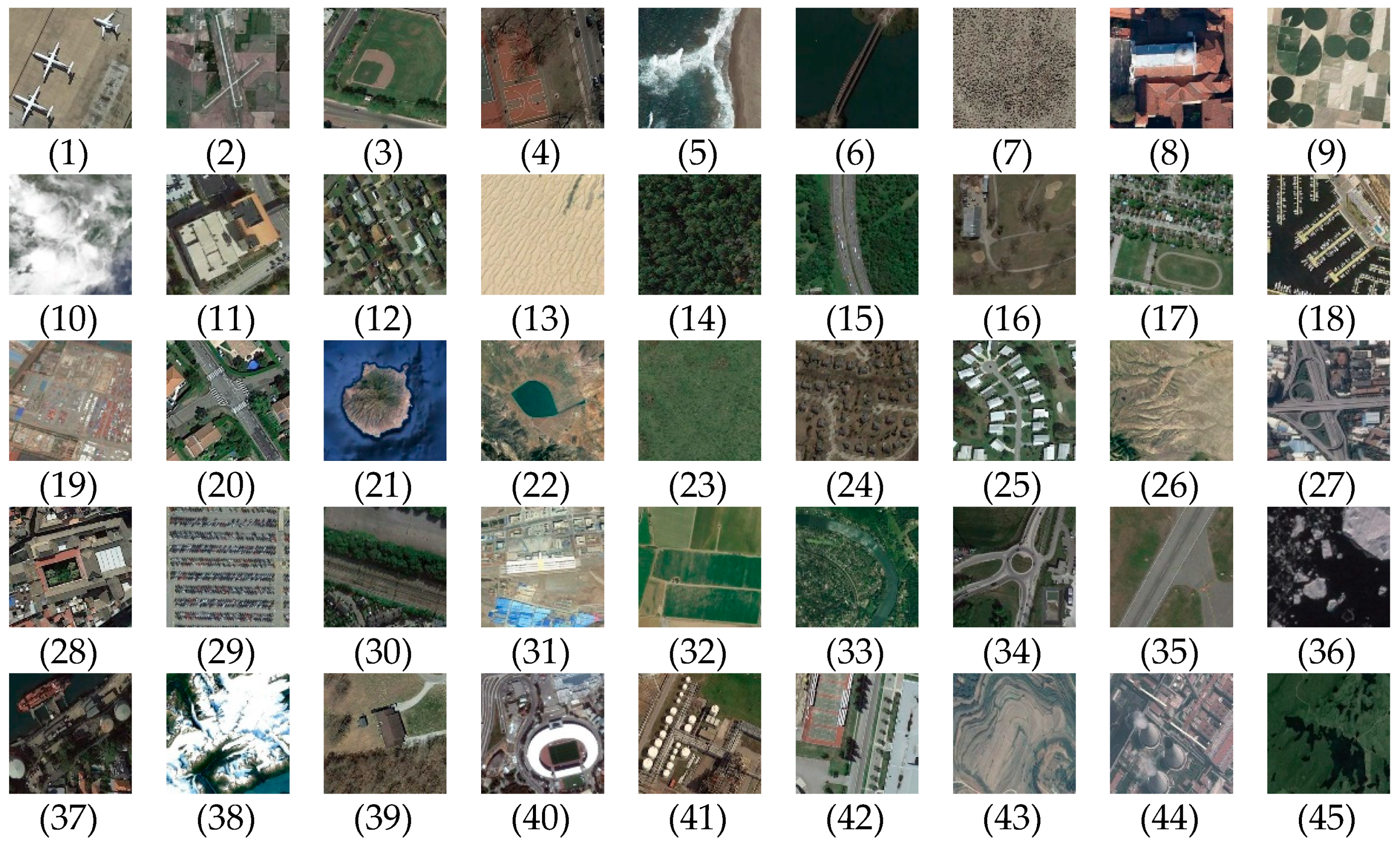
Figure 1.
Examples from the NWPU-RESIST45 dataset: (1) airplane, (2) airport, (3) baseball diamond, (4) basketball court, (5) beach, (6) bridge, (7) chaparral, (8) church, (9) circular farmland, (10) cloud, (11) commercial area, (12) dense residential, (13) desert, (14) forest, (15) freeway, (16) golf course, (17) ground track field, (18) harbor, (19) industrial area, (20) intersection, (21) island, (22) lake, (23) meadow, (24) medium residential, (25) mobile home park, (26) mountain, (27) overpass, (28) palace, (29) parking lot, (30) railway, (31) railway station, (32) rectangular farmland, (33) river, (34) roundabout, (35) runway, (36) sea ice, (37) ship, (38) snowberg, (39) sparse residential, (40) stadium, (41) storage tank, (42) tennis court, (43) terrace, (44) thermal power station, (45) wetland.
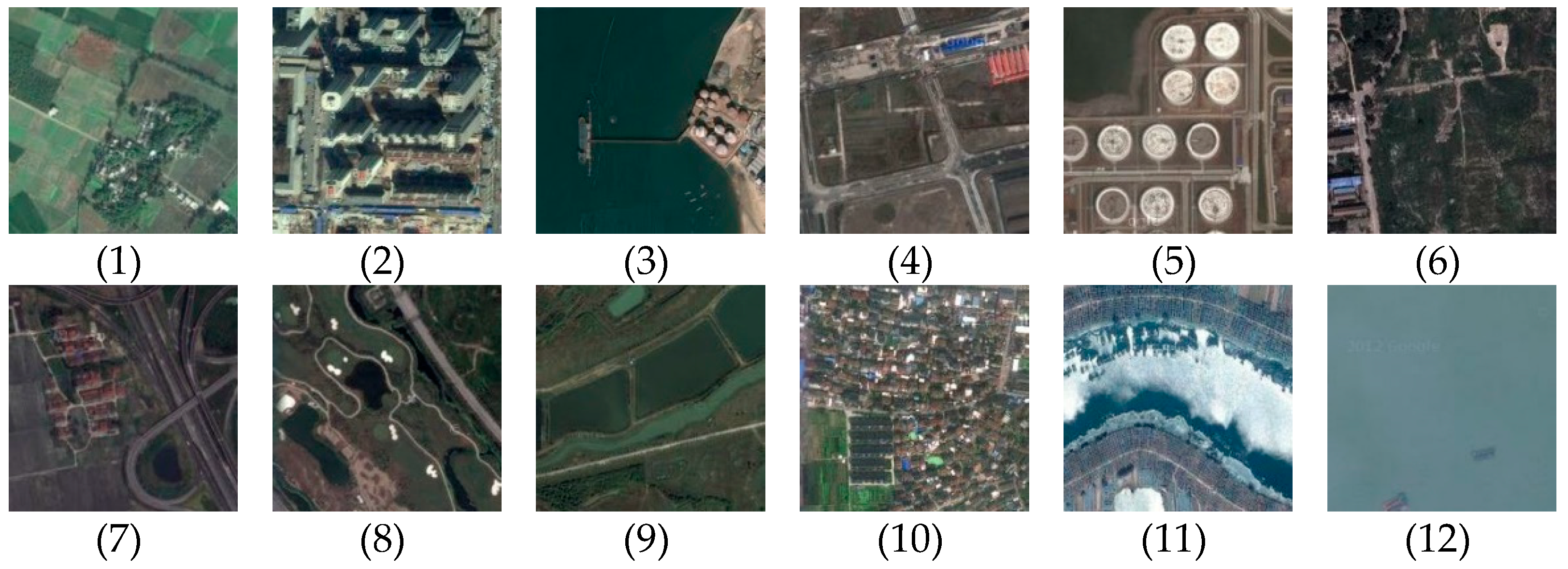
Figure 2.
Examples from the SIRI-WHU dataset: (1) farmland, (2) business quarters, (3) ports, (4) idle land, (5) industrial areas, (6) grasslands, (7) overpasses, (8) parking lots, (9) ponds, (10) residential areas, (11) rivers, (12) water.
Figure 2.
Examples from the SIRI-WHU dataset: (1) farmland, (2) business quarters, (3) ports, (4) idle land, (5) industrial areas, (6) grasslands, (7) overpasses, (8) parking lots, (9) ponds, (10) residential areas, (11) rivers, (12) water.
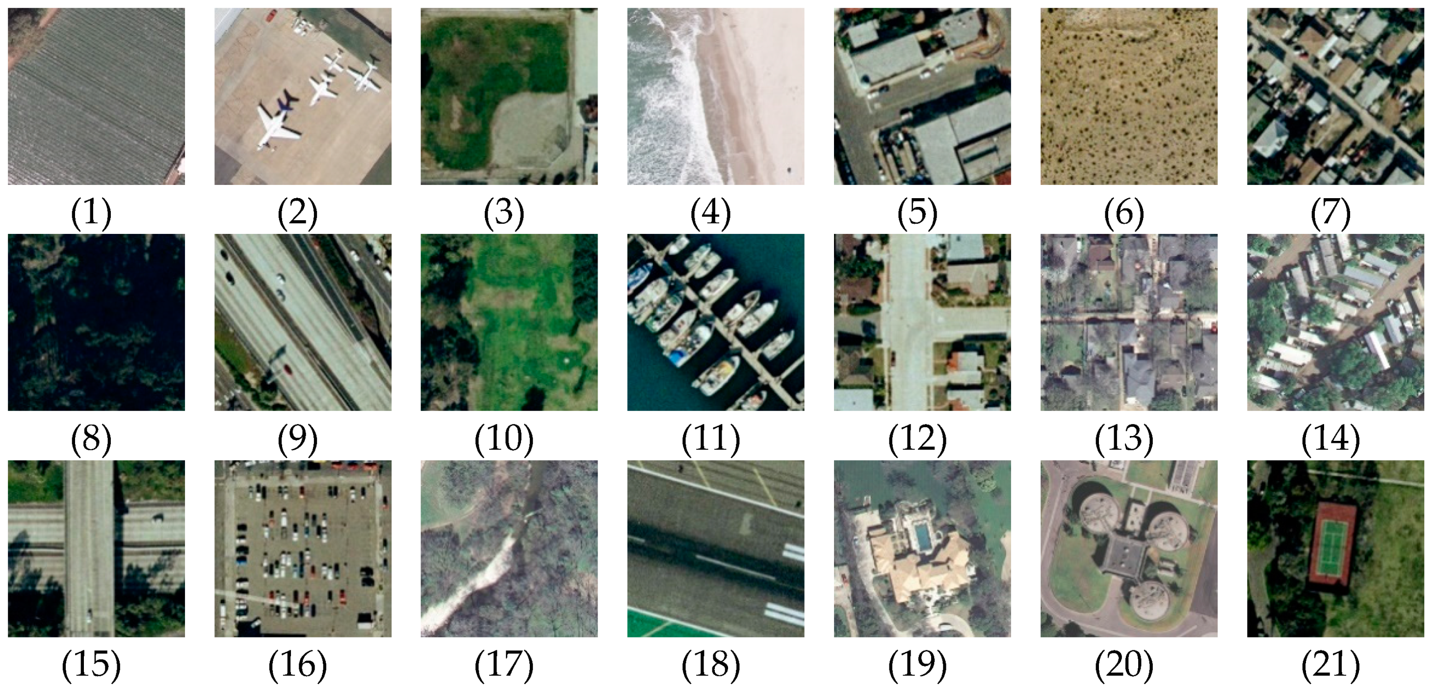
Figure 3.
Examples from the UC Merced dataset: (1) agricultural, (2) airplane, (3) baseball diamond, (4) beach, (5) buildings, (6) chaparral, (7) dense residential, (8) forest, (9) freeway, (10) golf course, (11) harbor, (12) intersection, (13) medium-density residential, (14) mobile home park, (15) overpass, (16) parking lot, (17) river, (18) runway, (19) sparse residential, (20) storage tanks, (21) tennis courts.
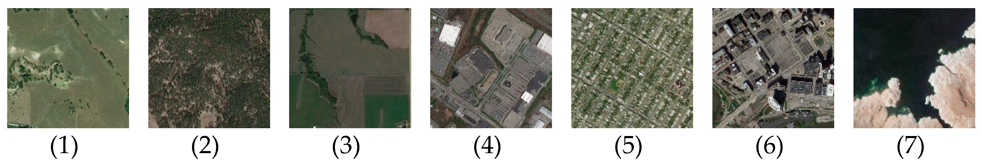
Figure 4.
Examples from the RSSCN7 dataset: (1) grassland, (2) forest, (3) farmland, (4) parking lot, (5) residential region, (6) industrial region, (7) river and lake.
Figure 4.
Examples from the RSSCN7 dataset: (1) grassland, (2) forest, (3) farmland, (4) parking lot, (5) residential region, (6) industrial region, (7) river and lake.
Figure 5.
Cross-domain scene classification process based on the SGNAS.
Figure 5.
Cross-domain scene classification process based on the SGNAS.
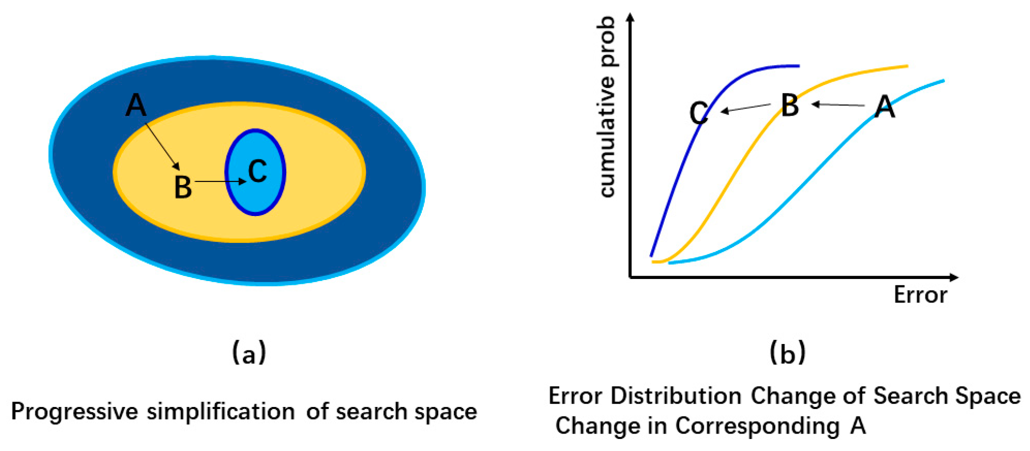
Figure 6.
The design process of the architecture search space in this paper.
Figure 6.
The design process of the architecture search space in this paper.
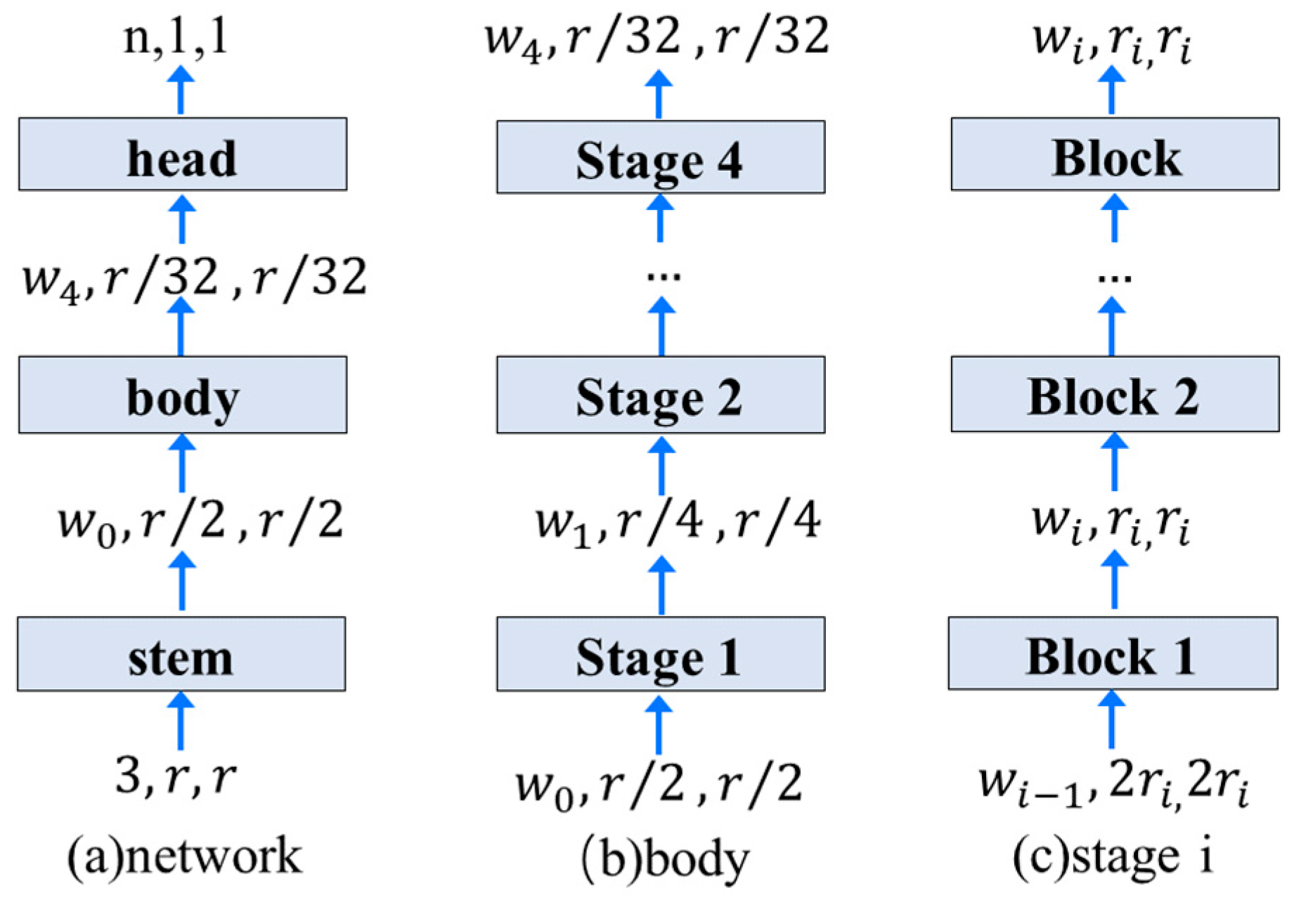
Figure 7.
The basic network design of the initial search space constructed in this paper.
Figure 7.
The basic network design of the initial search space constructed in this paper.
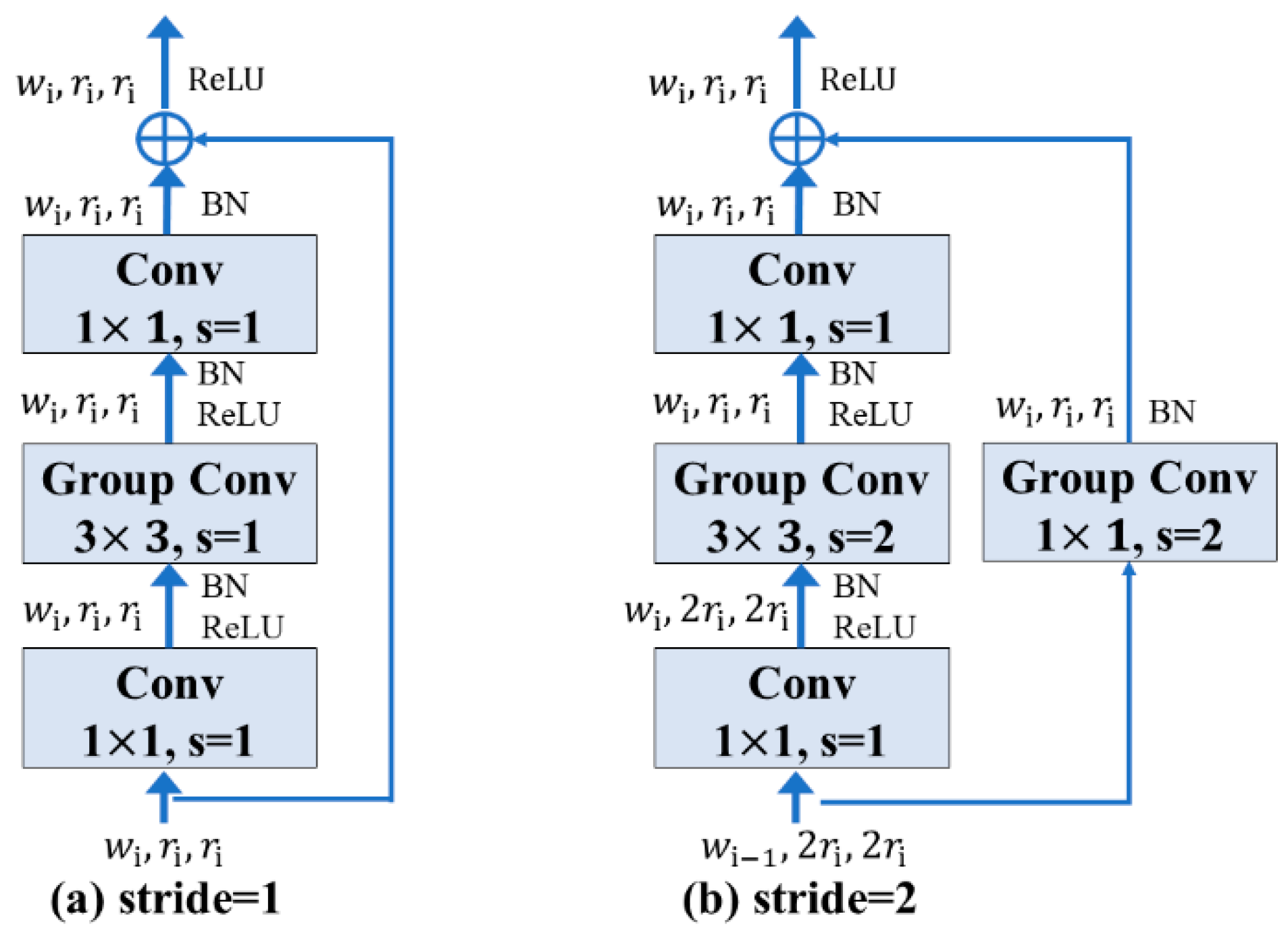
Figure 8.
The structure of residual bottleneck block. (a) Case of stride = 1, (b) Case of stride = 2.
Figure 8.
The structure of residual bottleneck block. (a) Case of stride = 1, (b) Case of stride = 2.
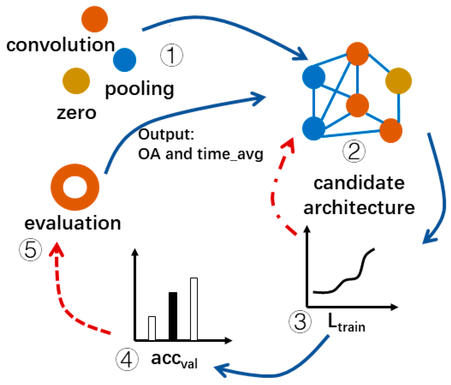
Figure 9.
The process of the architecture search in this paper.
Figure 9.
The process of the architecture search in this paper.
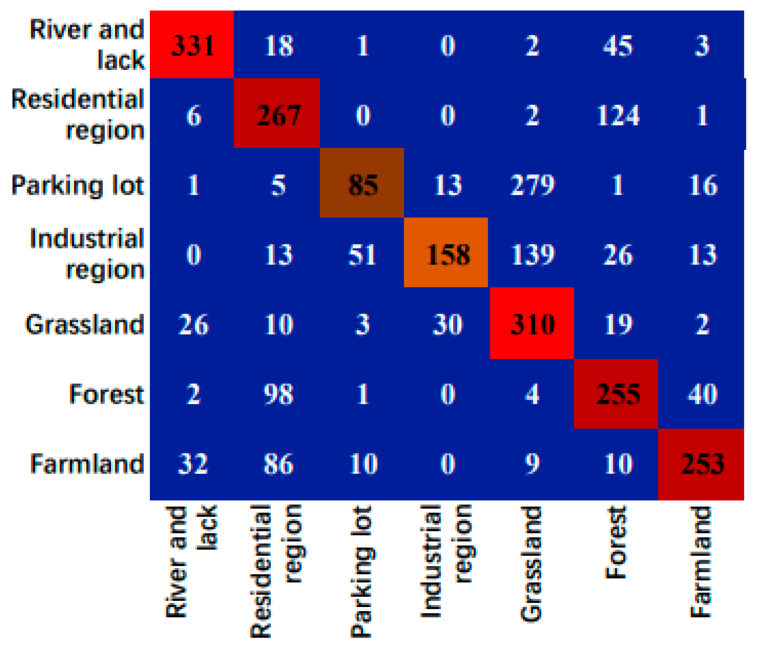
Figure 10.
Confusion matrix of the cross-domain scene classification results for UCM→RSSCN7.
Figure 10.
Confusion matrix of the cross-domain scene classification results for UCM→RSSCN7.
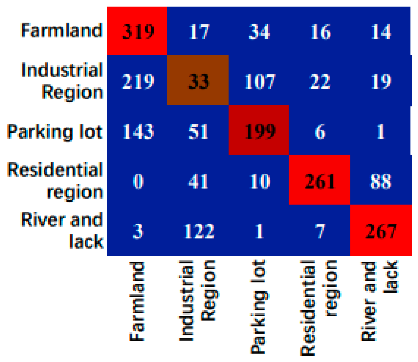
Figure 11.
Confusion matrix of cross-domain scene classification results in SIRI-WHU→RSSCN7.
Figure 11.
Confusion matrix of cross-domain scene classification results in SIRI-WHU→RSSCN7.
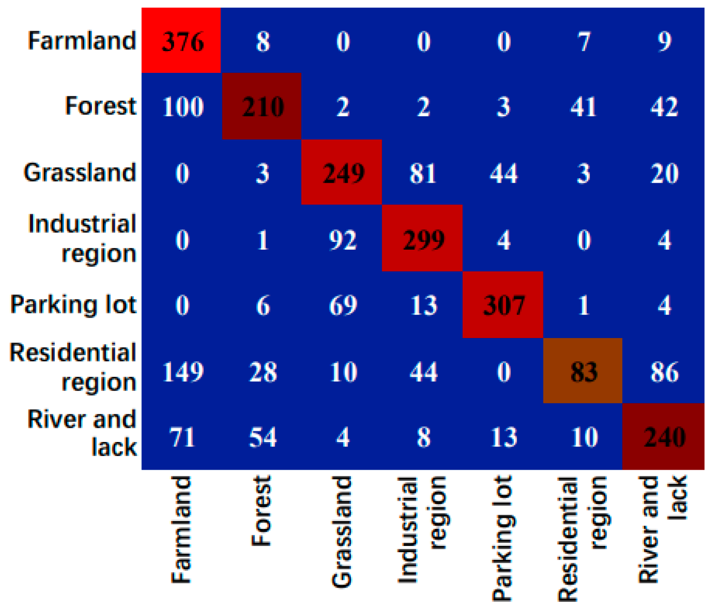
Figure 12.
Confusion matrix of the cross-domain scene classification results for NWPU-RESIST45→RSSCN7.
Figure 12.
Confusion matrix of the cross-domain scene classification results for NWPU-RESIST45→RSSCN7.
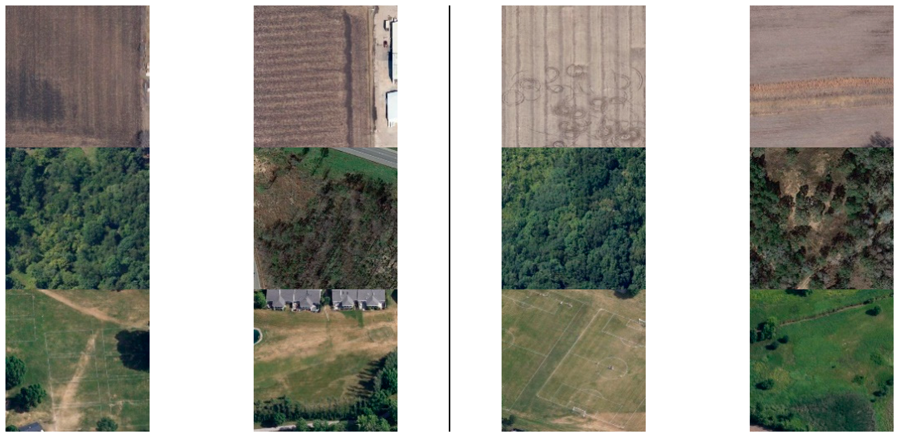
Figure 13.
Randomly sampled images from UCM, SIRI-WHU, NWPU-RESIST45, and RSSCN7 datasets. The first, second, third and fourth rows of (a) correspond to the scene classes of golf course in UCM dataset, farmland in SIRI-WHU dataset, parking lot in SIRI-WHU dataset, and farmland in the NWPU-RESIST45 dataset. The first, second, third, and fourth rows of (b) correspond to the scene classes of parking lot, industrial region, industrial region, and residential region in the RSSCN7 dataset.
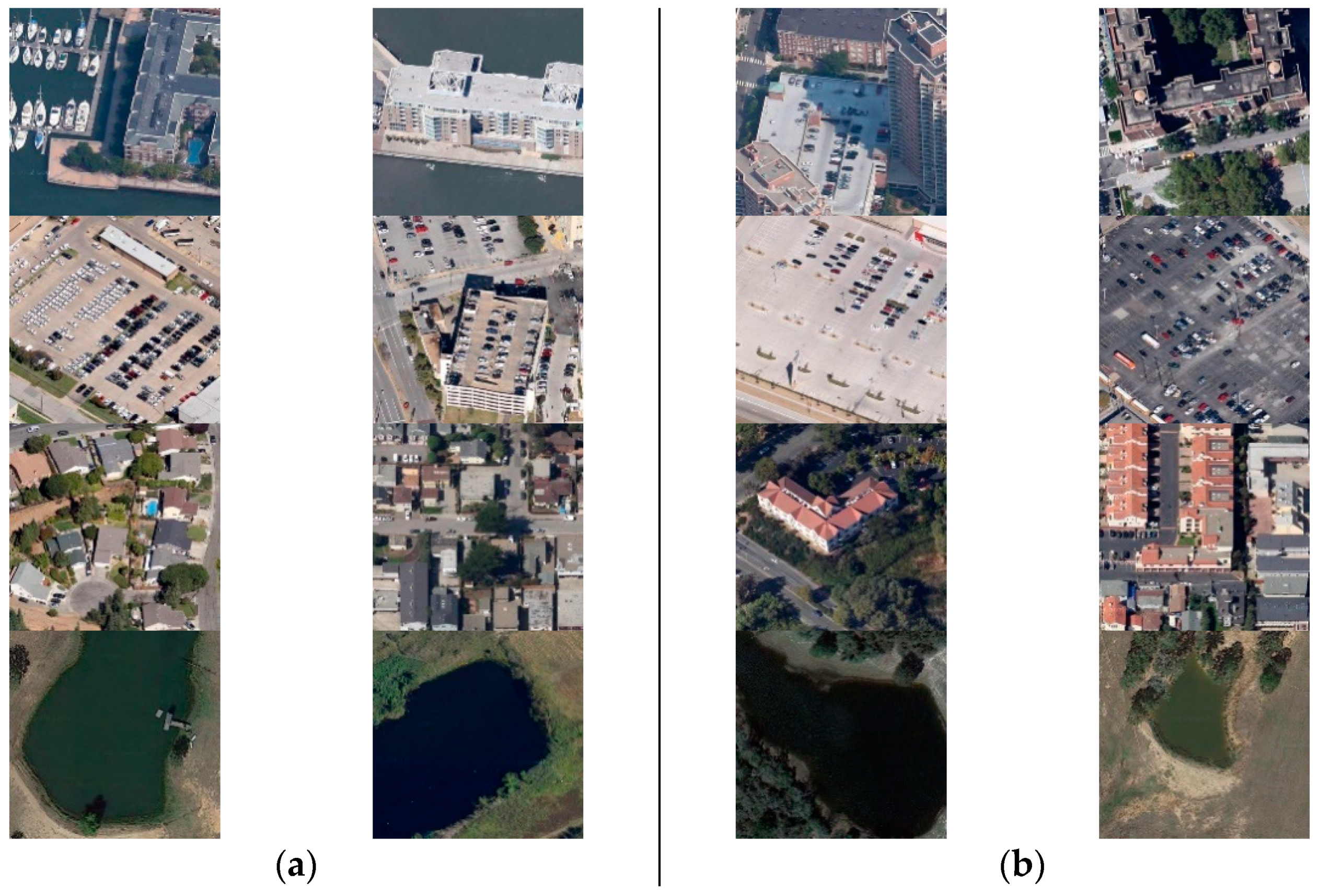
Figure 14.
Some of the classification results of SGNAS and other models in the cross-domain scene dataset of UCM→RSSCN7. The first, second, third, fourth, fifth, sixth, and seventh rows correspond to the scene classes of farmland, forest, grassland, industrial region, parking lot, residential region, and river and lake in the RSSCN7 dataset, respectively. (a) Correctly classified images for all models. (b) Images classified correctly by SGNAS, but incorrectly classified by other models were used for comparison.
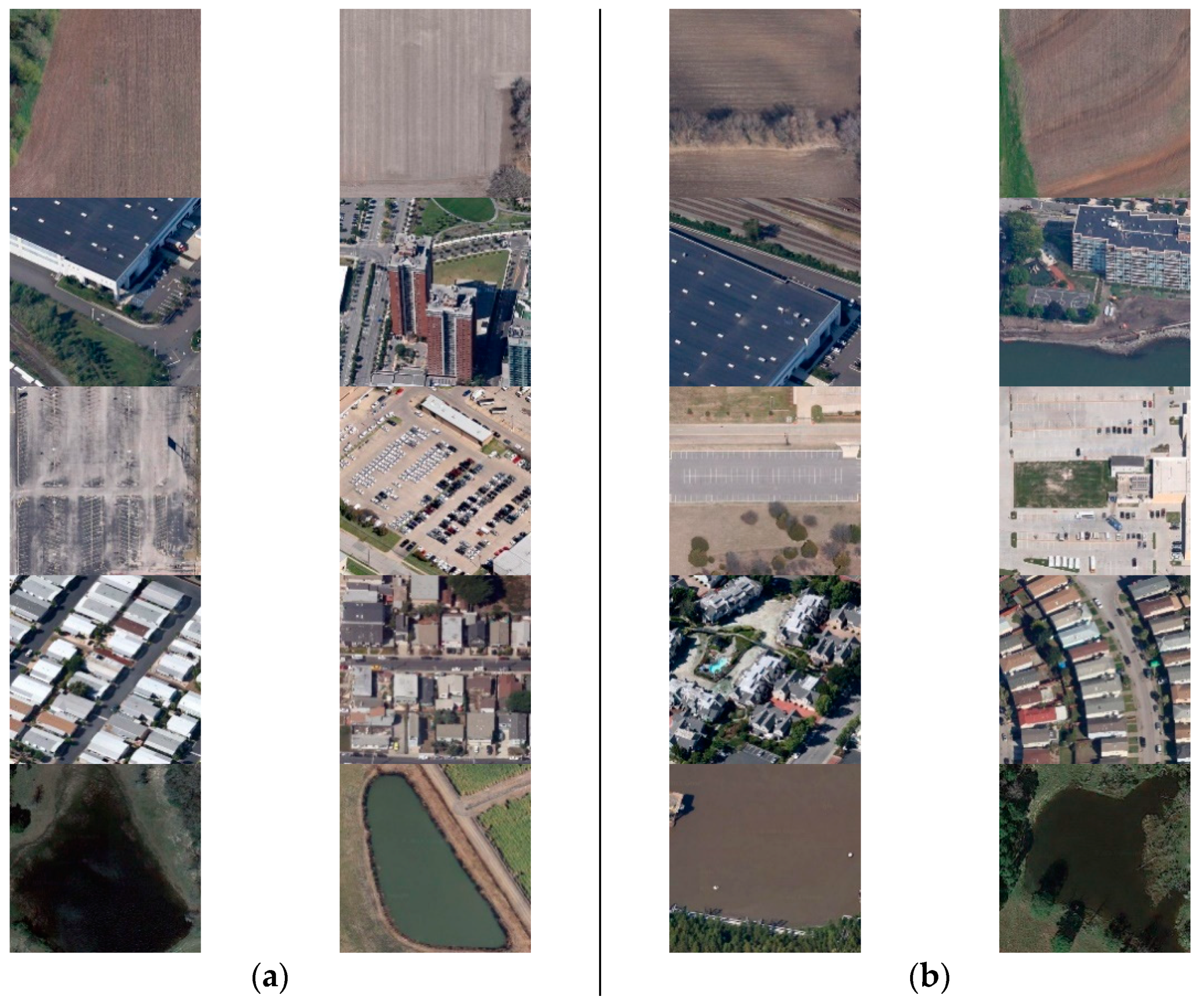
Figure 15.
Some of the classification results of SGNAS and other models in the cross-domain scene dataset of SIRI-WHU→RSSCN7. The first, second, third, fourth, and fifth rows correspond to the scene classes of farmland, industrial region, parking lot, residential region, and river and lake in the RSSCN7 dataset, respectively. (a) Correctly classified images for all the models. (b) Images classified correctly by SGNAS, but incorrectly classified by other models were used for comparison.
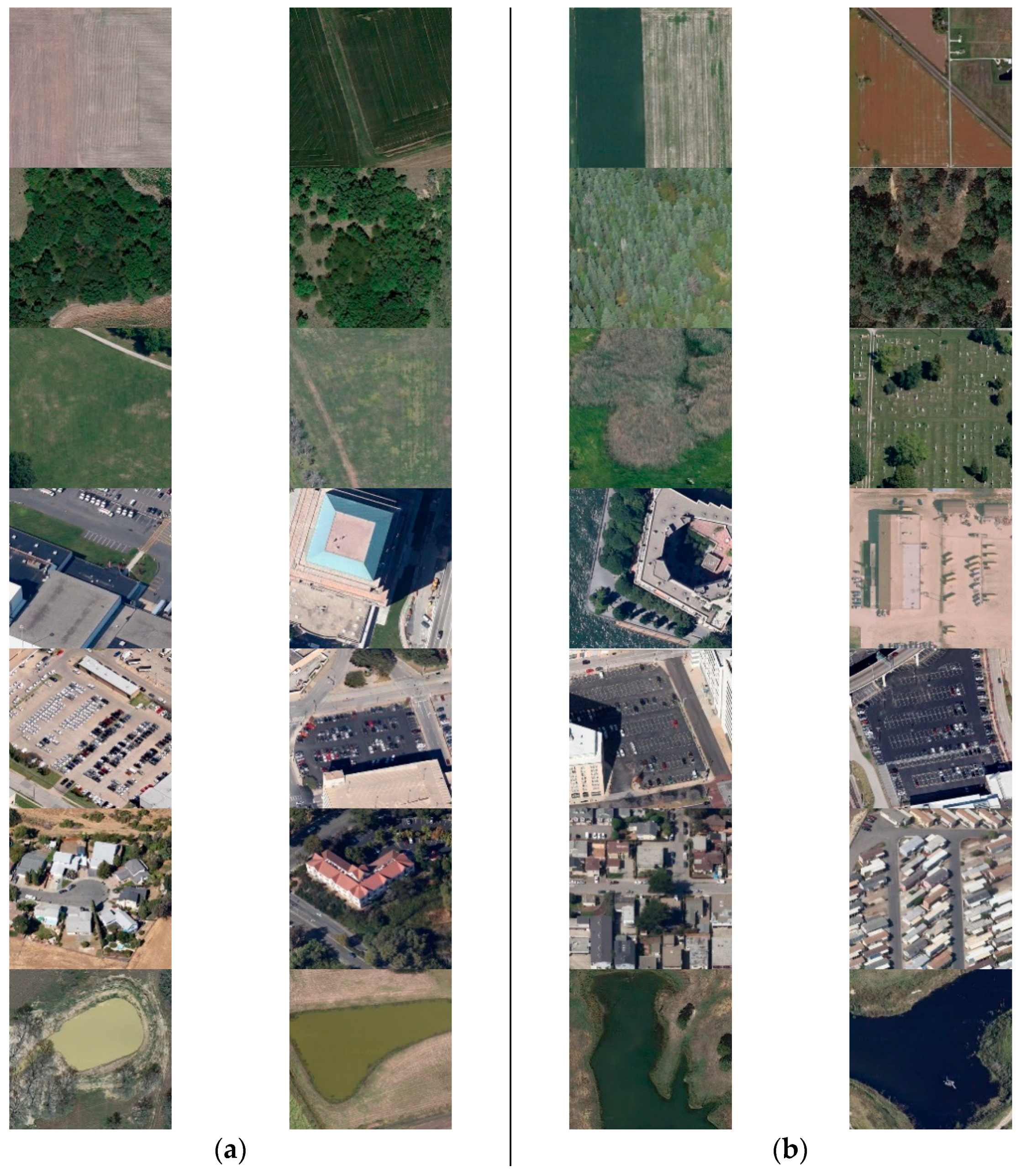
Figure 16.
Some of the classification results of SGNAS and other models in the cross-domain scene data set of NWPU-RESIST45→RSSCN7. The first, second, third, fourth, fifth, sixth, and seventh rows correspond to the scene classes of farmland, forest, grassland, industrial region, parking lot, residential region, and river and lake in the RSSCN7 dataset, respectively. (a) Correctly classified images for all the models. (b) Images classified correctly by SGNAS, but incorrectly classified by other models were used for comparison.
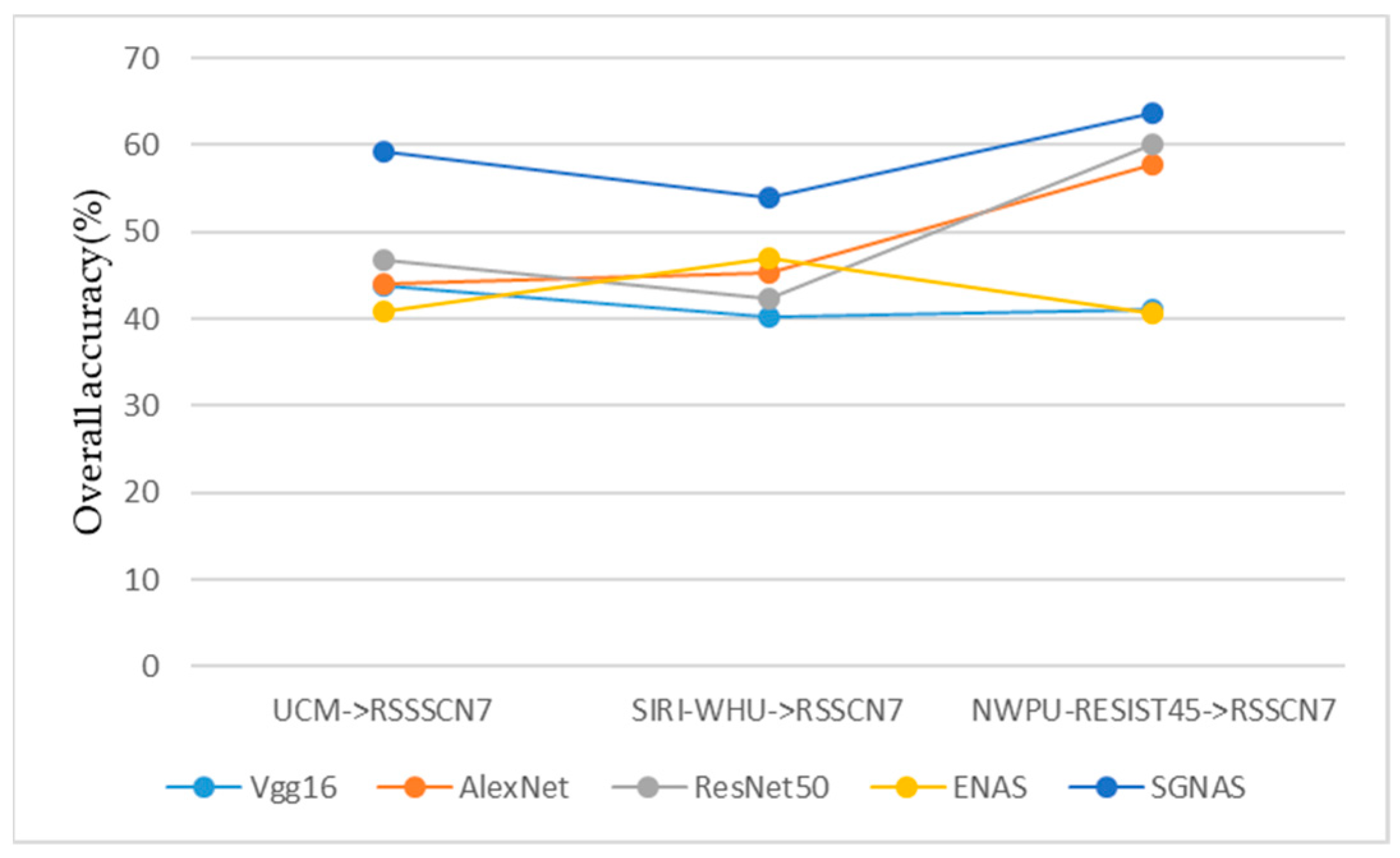
Figure 17.
Overall accuracy values of each model on three cross-domain scenarios.
Figure 17.
Overall accuracy values of each model on three cross-domain scenarios.
Table 1.
Overall accuracy and inference time of cross-domain scene classification of different models on UCM→RSSCN7.
Table 1.
Overall accuracy and inference time of cross-domain scene classification of different models on UCM→RSSCN7.
| Models | OA (%) | Time_infer (s) |
|---|
| Vgg16 | 43.79 | 23 |
| AlexNet | 44.00 | 12 |
| ResNet50 | 46.71 | 9 |
| ENAS | 40.82 | 46 |
| SGNAS | 59.25 | 8 |
Table 2.
Accuracy of various scenes in cross-domain scene classification of the UCM and RSSCN7 datasets of SGNAS.
Table 2.
Accuracy of various scenes in cross-domain scene classification of the UCM and RSSCN7 datasets of SGNAS.
| Class | Accuracy (%) |
|---|
| River and lake | 82.75 |
| Residential region | 66.75 |
| Parking lot | 21.25 |
| Industrial region | 39.50 |
| Grassland | 77.50 |
| Forest | 63.75 |
| Farmland | 63.25 |
Table 3.
Overall accuracy and inference time of the cross-domain scene classification of different models for SIRI-WHU→RSSCN7.
Table 3.
Overall accuracy and inference time of the cross-domain scene classification of different models for SIRI-WHU→RSSCN7.
| Models | OA (%) | Time_infer (s) |
|---|
| Vgg16 | 40.30 | 37 |
| AlexNet | 45.25 | 11 |
| ResNet50 | 42.40 | 142 |
| ENAS | 46.95 | 137 |
| SGNAS | 53.95 | 40 |
Table 4.
Accuracy of various scenes in the cross-domain scene classification of the SIRI-WHU and RSSCN7 datasets of the SGNAS.
Table 4.
Accuracy of various scenes in the cross-domain scene classification of the SIRI-WHU and RSSCN7 datasets of the SGNAS.
| Class | Accuracy (%) |
|---|
| Farmland | 79.75 |
| Industrial region | 8.25 |
| Parking lot | 49.75 |
| Residential region | 65.25 |
| River and lake | 66.75 |
Table 5.
Overall accuracy and inference time of the cross-domain scene classification of different models for NWPU-RESIST45→RSSCN7.
Table 5.
Overall accuracy and inference time of the cross-domain scene classification of different models for NWPU-RESIST45→RSSCN7.
| Models | OA (%) | Time_infer (s) |
|---|
| Vgg16 | 41.11 | 678 |
| AlexNet | 57.82 | 97 |
| ResNet50 | 60.04 | 390 |
| ENAS | 40.64 | 860 |
| SGNAS | 63.56 | 158 |
Table 6.
Accuracy of various scenes in the cross-domain scene classification of the NWPU-RESIST45 and RSSCN7 datasets of the SGNAS.
Table 6.
Accuracy of various scenes in the cross-domain scene classification of the NWPU-RESIST45 and RSSCN7 datasets of the SGNAS.
| Class | Accuracy (%) |
|---|
| Farmland | 91.75 |
| Forest | 52.50 |
| Grassland | 62.25 |
| Industrial region | 74.75 |
| Parking lot | 76.75 |
| Residential region | 20.75 |
| River and lake | 60.00 |


