
Research on Polarized Multi-Spectral System and Fusion Algorithm for Remote Sensing of Vegetation Status at Night


Department of Precision Mechanical Engineering, Shanghai University, Shanghai 200444, China
*
Author to whom correspondence should be addressed.
Remote Sens. 2021, 13(17), 3510; https://0-doi-org.brum.beds.ac.uk/10.3390/rs13173510
Submission received: 2 August 2021
/
Revised: 1 September 2021
/
Accepted: 1 September 2021
/
Published: 4 September 2021
(This article belongs to the Special Issue Crop Disease Detection Using Remote Sensing Image Analysis)
Abstract
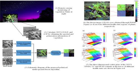
:The monitoring of vegetation via remote sensing has been widely applied in various fields, such as crop diseases and pests, forest coverage and vegetation growth status, but such monitoring activities were mainly carried out in the daytime, resulting in limitations in sensing the status of vegetation at night. In this article, with the aim of monitoring the health status of outdoor plants at night by remote sensing, a polarized multispectral low-illumination-level imaging system (PMSIS) was established, and a fusion algorithm was proposed to detect vegetation by sensing the spectrum and polarization characteristics of the diffuse and specular reflection of vegetation. The normalized vegetation index (NDVI), degree of linear polarization (DoLP) and angle of polarization (AOP) are all calculated in the fusion algorithm to better detect the health status of plants in the night environment. Based on NDVI, DoLP and AOP fusion images (NDAI), a new index of night plant state detection (NPSDI) was proposed. A correlation analysis was made for the chlorophyll content (SPAD), nitrogen content (NC), NDVI and NPSDI to understand their capabilities to detect plants under stress. The scatter plot of NPSDI shows a good distinction between vegetation with different health levels, which can be seen from the high specificity and sensitivity values. It can be seen that NPSDI has a good correlation with NDVI (coefficient of determination R2 = 0.968), PSAD (R2 = 0.882) and NC (R2 = 0.916), which highlights the potential of NPSDI in the identification of plant health status. The results clearly show that the proposed fusion algorithm can enhance the contrast effect and the generated fusion image will carry richer vegetation information, thereby monitoring the health status of plants at night more effectively. This algorithm has a great potential in using remote sensing platform to monitor the health of vegetation and crops.
1. Introduction
Vegetation plays an important role in the global ecosystem [1], but natural disasters such as drought, pests and diseases affect their growth of greatly, even leading to their death. In the past 30 years, monitoring the health status of vegetation via remote sensing has been applied in many areas successfully, such as the analysis of crop diseases and pests, monitoring forest coverage and vegetation growth status, etc. However, such remote sensing-based activities are mainly carried out during the daytime, with limitations in sensing the vegetation status at night. Crop diseases and pests are important factors for analyzing crop yields. For example, Spodoptera frugiperda, as one kind of nocturnal animal, spreads extremely fast and seriously threatens human food security [2]. Thus, it is necessary to monitor them efficiently with state-of-the-art techniques. Therefore, it is essential and important to develop an effective and accurate method to monitor the health status of vegetation in the night environment.
With the development of remote sensing technologies based on multiple platforms (space, air and ground), various remote sensing-based methods are used to monitor plant health [3,4,5,6,7,8,9,10,11]. For the optical remote sensing methods, the visible and near-infrared wave bands are mainly used for analysis of plant diseases and insect pests [12,13,14,15,16,17,18,19,20,21]. As the vegetation of different healthy status have different absorption and reflection characteristics at different wavelengths, various vegetation indices (VIS) with visible and near-infrared wave bands have been developed to monitor vegetation growth and health [22], such as the normalized vegetation index (NDVI, Rouse et al. 1973) [23], soil-adjusted vegetation index (SAVI, Huete 1988) [24], modified soil-adjusted vegetation index (MSAVI, Qi et al. 1994) [25] and normalized difference water index (NDWI, Gao 1996) [26]. More and more indices are being developed to study and analyze the crop damage caused by pests with remote sensing.
For the ground-based remote sensing technologies, typically, handheld instruments are widely used monitoring crop diseases [27], and tower-based platforms [28,29,30] and other huge near-ground platforms are used to obtain crop spectral information under different disease states at the leaf and canopy scales. For example, Graeff et al. (2006) [31] used a digital imager (Leica S1 Pro, Leica, Wetzlar, Germany) to analyze the spectrum of wheat leaves infected with powdery mildew and take-all disease, finding this disease resulted in strong spectral response at 490 nm, 510 nm, 516 nm, 540 nm, 780 nm and 1300 nm. Yang et al. (2009) [32] used a hand-held Cropscan radiometer and found that it was feasible to use the ratio vegetation index (400/450 nm and 950 nm/450 nm) to identify and distinguish plants infested by green aphids and Russian wheat aphids. Liu et al. (2010) [33] used a portable spectrophotometer (Field Spec Full Range, ASD Inc., Boulder, CO, USA) to analyze the spectral characteristics of Rice Panicles and found that there was a correlation between the reflectance change in the 450–850-nm band and rice glume blight disease. In addition, Prabhakar et al. (2011) [34] found that the spectral reflectance of healthy plants was significantly different from the plants infested by leafhoppers in the visible and near-infrared bands with a Hi-Res spectroradiometer (ASD Inc., Boulder, CO, USA; spectral range: 350–2500 nm), and the new leaf hopper index (LHI) was applied to monitor the severity of leafhopper. Prabhakar et al. (2013) [35] used a Hi-Res spectroradiometer (ASD Inc., Boulder, CO, USA; spectral range: 350–2500 nm) for the experiment and found that the most sensitive bands to cotton mealybug infestation were concentrated at 492 nm, 550 nm, 674 nm, 768 nm and 1454 nm, and a new cotton mealybug Stress Index (MSI) was developed.
Besides ground-based remote sensing technologies, various air and space-based remote sensing technologies have been developed and widely applied to the monitoring of plant diseases and insect pests, with the advantages of good temporal, spatial and spectral resolutions. In general, the airborne platform used for monitoring crop diseases can be integrated with different sensors, such as an imaging camera, multispectral/hyperspectral spectrometer, infrared camera, lidar and other detection systems [36,37]. For example, Yang et al. (2010) [38] used high-resolution multispectral and hyperspectral aerial image data to extract the occurrence range of cotton root rot and indicated that multispectral data was promising for large-scale disease monitoring. Calder ó n et al. (2013) [39] used UAV with the multispectral camera and thermal infrared camera to diagnose the verticillium wilt of olive trees. Sanches et al. (2014) [40] calculated a new Plant Stress Detection Index (PSDI) from the chlorophyll characteristic center (680 nm) and green edge (560 nm and 575 nm) with an airborne imaging spectrometer (ProSpecTIR-VS) and the continuum division method, showing this index could be used for an analysis of the canopy status successfully. Lehmann et al. (2015) [41] analyzed the UAV multi-spectral images with object-based image processing methods to monitor the pests of oak trees. For the cases of space-based remote sensing applications, Yuan et al. (2016) [42] proposed a monitoring method with the help of SPOT-6 images to analyze the occurrence of Wheat Powdery Mildew in the Guanzhong area of Shaanxi Province, with an accuracy of 78%. Chen et al. (2018) [43] applied high-resolution multi-spectral satellite images to monitor wheat rust, with a classification accuracy of 90%. Zheng et al. (2018) [44] used the Sentinel-2 Multispectral Instrument (MSI) to distinguish the severity of yellow rust infection in the winter and proposed the Red Edge Disease Stress Index (REDSI) to detect yellow rust infections of different severities. Meiforth et al. (2020) [45] used the WorldView-2 (WV2) satellite and LiDAR data to detect the stress of kauri canopies in New Zealand. The results showed that this method can be used to monitor kauri canopies economically and efficiently in a large area. Li et al. (2021) [46] developed a machine learning model to analyze the vegetation growth by retrieving NDVI from the satellite sensor.
It is clear that vegetation indices based on different remote sensing platforms play an important role in monitoring the status of crops. When the polarization information is supplemented, more complex and accurate indices and models can be developed, and the polarization shows directional characteristics when light interacts with the vegetation [47,48]. Polarization has attracted many researchers to study remote sensing together with polarization information. For example, Vanderbilt et al. pointed out that polarization was affected by vegetation canopy morphology and leaf surface characteristics [49,50]. Since vegetation canopy morphology and leaf surface characteristics are affected by stress, activity and the growth stage, polarization-based parameters, such as the degree of linear polarization (DoLP) of vegetation, can reflect such information well [51]. Compared to traditional remote sensing methods without polarization information, polarization-based remote sensing can provide vegetation canopy information, such as the structure of leaf layers [52] and the emergence of panicles above canopies [53]. Theoretical and practical research indicates the possibility of detecting the geometry of vegetation canopies with polarization [54,55]. Besides, many researchers have measured various leaves in an extensive way [56,57,58,59,60]. Hu et al. studied polarization imaging in low-light environments [61]. For the above-mentioned research, it is worth noting that the researchers are still in the phase of ground experiments in studying remote sensing technologies.
It is shown that the health of vegetation can be monitored successfully with different remote sensing technologies, and various methods have been carried out during the daytime. However, limited efforts have been done in monitoring the health of vegetation at night, which requires high-sensitivity imaging equipment but is quite important and necessary. In this paper, a ground-based remote sensing system is developed and used for monitoring the health of vegetation at night. Since polarization information can supplement traditional spectral imaging to develop more complex and accurate models for vegetation monitoring, in this paper, we developed a polarized multispectral low-illumination-level imaging system, which is used to record the spectral images of vegetation at 680 nm and 760 nm during the night, as well as the polarization images at 0°, 60° and 120°. Moreover, a fusion algorithm is proposed to improve the contrast of vegetation detection by fusing polarization images and spectral images of vegetation. The vegetation index (NDVI), degree of linear polarization (DoLP) and angle of polarization (AOP) are all calculated in the fusion algorithm for better detection of the health status of plants at night. In addition, a new index, the night plant status detection index (NPSDI), was calculated based on the fusion images of NDVI, DoLP and AOP. The index was compared with physiological parameters of plants, such as nitrogen content (NC) and SPAD, to assess the applicability of the fusion algorithm for the remote sensing of vegetation. Moreover, based on our novel ground-based remote sensing research, it is promising to transform the platform into air and space-based ones for large-scale remote sensing applications in the future.
2. Materials and Methods
2.1. Plant Materials and Experimental Design
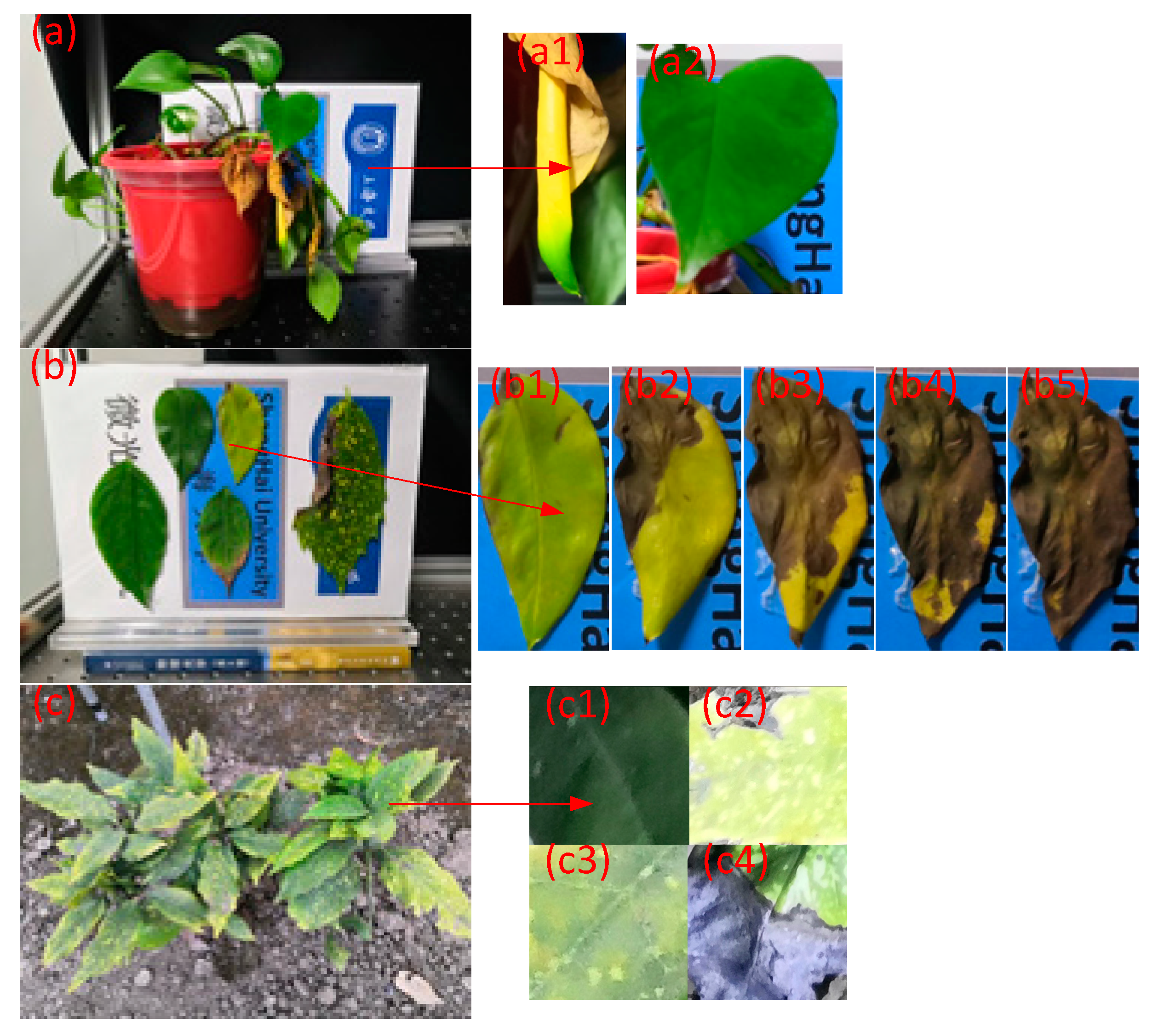
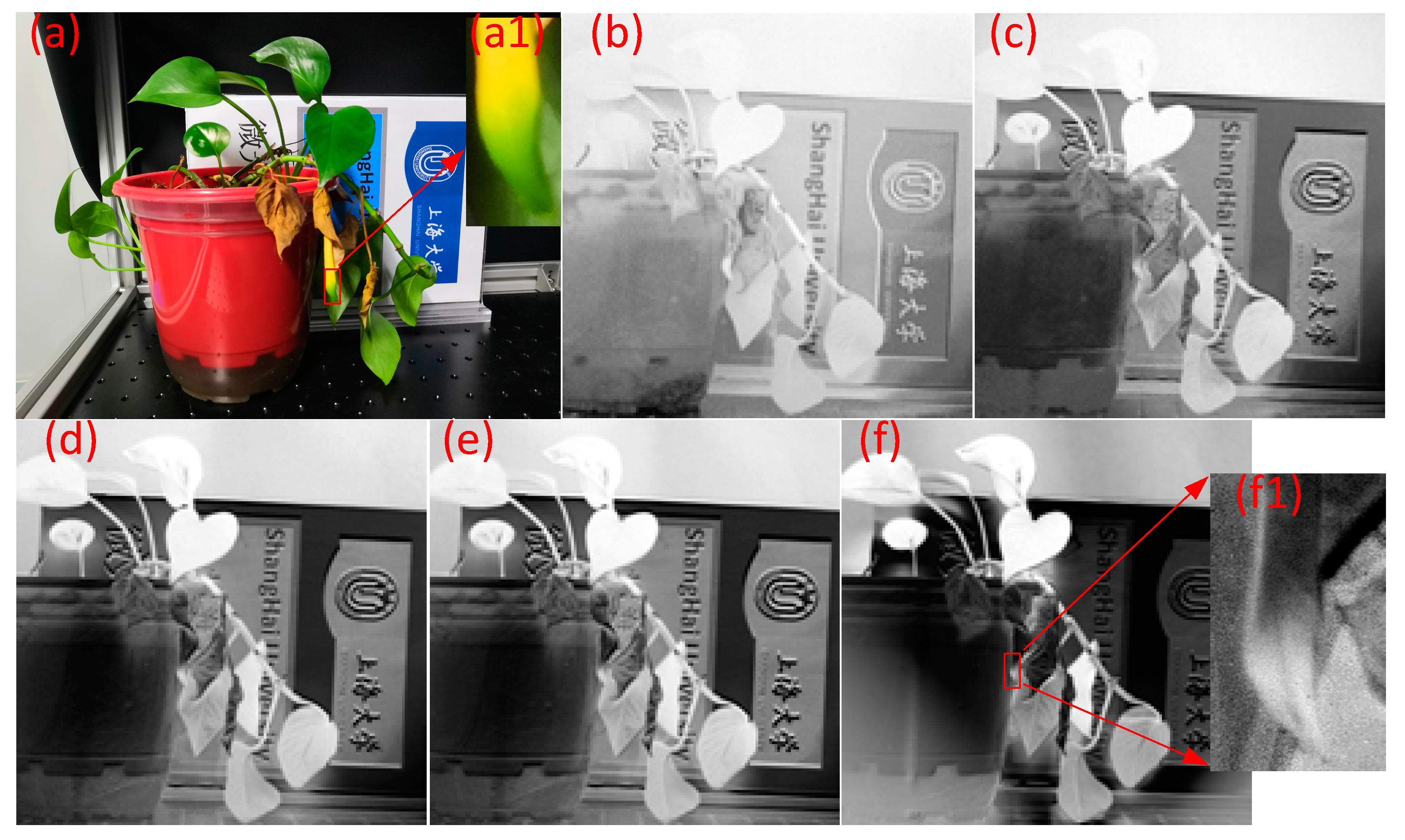
The spectral and polarization data analyzed in the study are from the leaves of plants on the campus of Shanghai University: spotted laurel (Aucuba japonica), money plant (Epipremnum aureum) and Malabar chestnut (Pachira aquatica). Figure 1a is a potted money plant in the laboratory, and Figure 1a1,a2 are the regions of interest for collecting vegetation index and polarization data, respectively. Figure 1b shows the leaves of spotted laurel, money plant and Malabar chestnut, and Figure 1b1–b5 shows the regions of interest collected by time series experiment at 3-day intervals. Figure 1c is a spotted laurel on the campus of Shanghai University, and Figure 1c1–c4 is defined as the healthy leaf region, level-2 stress leaf region, level-1 stress leaf region and withered leaf region, respectively.
Three experiments were designed in this paper, including: (1) an experiment was carried out under different illuminances of 0.01, 0.1, 0.5, 1 and 5 lux on a pot of money plant in a dark laboratory room, and the LED light group and LED controller were used to control the illumination of the dark room. The illumination was measured with a high-precision illuminometer (model: tes1330A, Taishi). (2) In the dark laboratory room, a time series experiment was carried out to collect data on the leaves of spotted laurel, money plant and Malabar chestnut every three days. Vegetation leaves were pasted on a display board printed at Shanghai University and placed in a dark room. The LED light group and LED controller were used to control the illumination of the dark room, and a high-precision illumination meter (model: tes1330A, Taishi) was used to measure the illumination. (3) An outdoor experiment was conducted on a spotted laurel on campus at night.
2.2. Polarized Multispectral for Low-Illumination-Level Imaging System
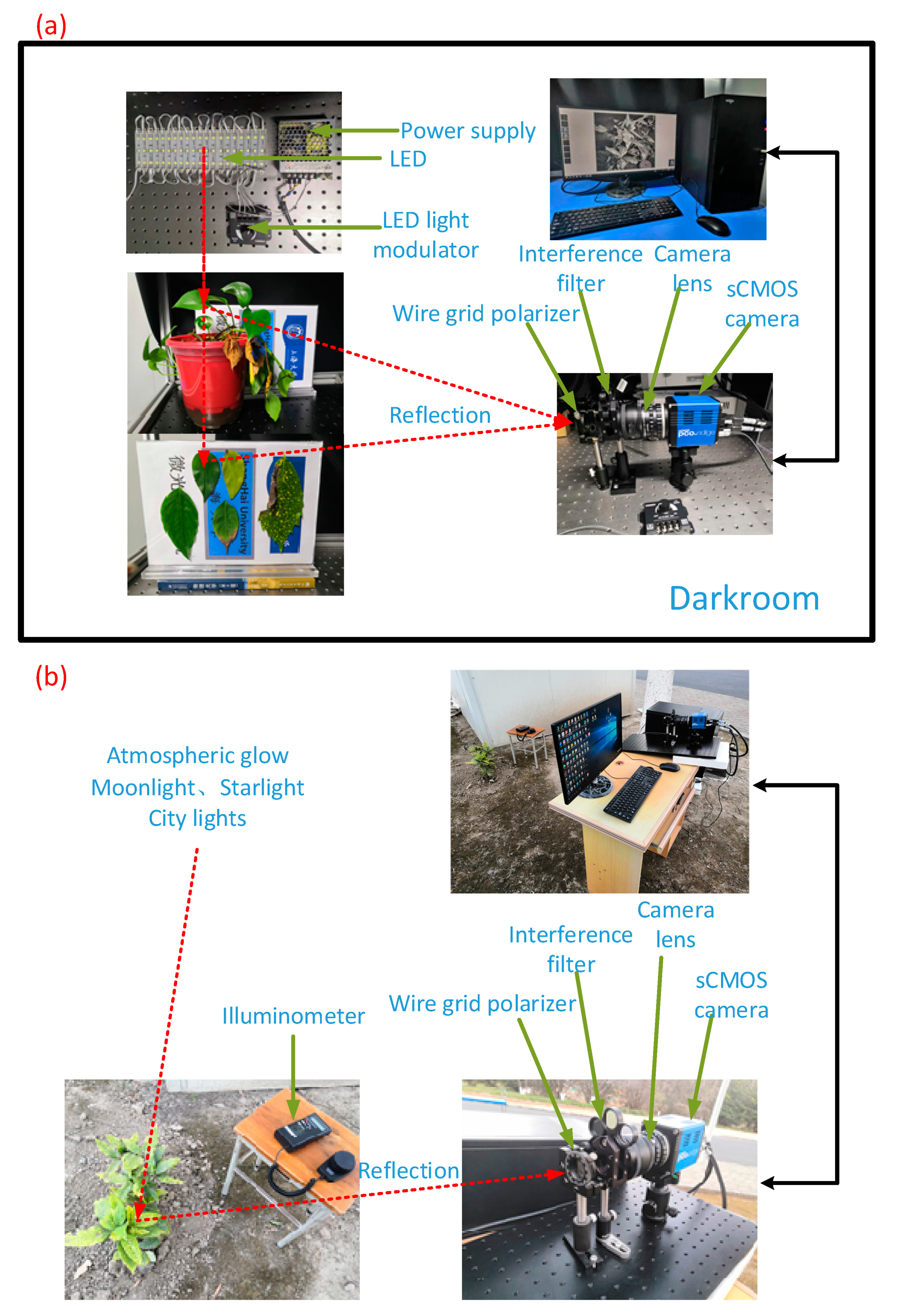
The polarized multispectral for low-illumination-level imaging system (PMSIS) developed for outdoor plant imaging at night consists of a scientific CMOS (SCMOS) monochrome camera with 2048 pixels × 2048 pixels (model: PCO. edge 4.2, PCO, GER), coupled to a Nikon MF 50-mm (1:1.8) fixed focus camera lens, narrow band interference filters fitted on a rotating filter mount and a linear polarizer fitted on a rotating polarizer mount (Figure 2). Blue (FF02-482/18-25) and green (FF02-520/28-25) band filters of Semrock and red (FB680-10) and near-infrared band (FB760-10) filters of Thorlabs were used. The camera was connected to a desktop computer, and the control and data acquisition were carried out through a Cameralink port.
As shown in Figure 2a, an indoor polarized multispectral for low-illumination-level imaging system was established. In order to simulate a night environment, the system was placed in a dark room made of optical shading material, and the shading rate of the dark room was greater than 99%. During the experiment, the illuminance of the dark room was controlled at 0.01, 0.1, 0.5, 1 and 5 lux, respectively (Note: dark night: 0.001–0.02 lux, moonlit night: 0.02–0.3 lux and cloudy indoor: 5–50 lux). The illuminance of the dark room was controlled by the LED lamp set and LED controller to carry out the experiment of monitoring the vegetation health status with different illuminances at night.
As shown in Figure 2b, an outdoor polarized multispectral for a low-illumination-level imaging system was built to conduct an outdoor night monitoring experiment on a spotted laurel. The time selected was from 8:00 at night. The ambient light included an atmospheric glow, starlight, moonlight and city light. The outdoor experiment location was on the campus of Shanghai University, Baoshan District, Shanghai (Season: Winter (Longitude: 121°24′1.95″, Latitude: 31°19′10.57″)), and the illuminance of 0.22 lux was actually measured with an illuminance meter.
2.3. Measurement of Chlorophyll and Nitrogen Content
The chlorophyll and nitrogen contents of plant leaves were measured with a handheld chlorophyll analyzer (Medium Kelvin, Model: TYS-4N). The chlorophyll analyzer can measure the relative chlorophyll (SPAD) and nitrogen contents (mg/g), leaf moisture (RH%) and temperature of plants instantly. In the test, two LED light sources emit light in two wavebands, one with a red light (center wavelength: 650 nm), the other with an infrared light (center wavelength: 940 nm). After penetrating the blade, the light is received and processed by the receiver, and finally, the SPAD value is calculated and displayed on the screen.
2.4. Image Acquisition and Analysis
Highly sensitive sCMOS cameras and filters with central bands of 482, 520, 680 and 760 nm were used to obtain the spectral data images of vegetation. Linear polarizers were used to obtain the polarization data images of vegetation with 0, 60 and 120 degrees. In this study, the spectral analysis focused on the absorption characteristics of chlorophyll in the central band near 680 nm and the reflection characteristics of chlorophyll in the central band near 760 nm, and the NDVI was used to retrieve the vegetation health status. The DoLP and AOP of vegetation were calculated using 0, 60 and 120-degree polarization images. Finally, the NDVI, DoLP and AOP were fused with the proposed fusion algorithm of night plant detection.
2.4.1. The Normalized Vegetation Index
The analysis based on the vegetation index has become a main way for scholars to study and practice the remote sensing detection of pests and diseases. So far, many different types of vegetation indices have been proposed one after another. With certain biological or physical and chemical significance, these vegetation indices are an important application form of the plant spectrum. At present, many studies have tried to establish the relationship between remote sensing information and the occurrence and degree of diseases and pests through various vegetation indices. In this study, the spectral image data of 680 nm and 760 nm in the central band were used to calculate the NDVI, of which the formula is as follows:
2.4.2. Polarization of Vegetation
When light is reflected from the leaf surface, its spectral characteristics will be affected by the element composition of the leaf surface, and its polarization characteristics will be affected by the characteristics of the leaf surface [62]. Polarization [63] and multispectral imaging can provide complementary information for vegetation detection. However, few people currently propose to fuse the information of polarization and spectral imaging to obtain better vegetation detection results. Therefore, this paper introduces polarization into vegetation detection and integrates it with the vegetation index to improve the detection of the vegetation health status.
Stokes formula:
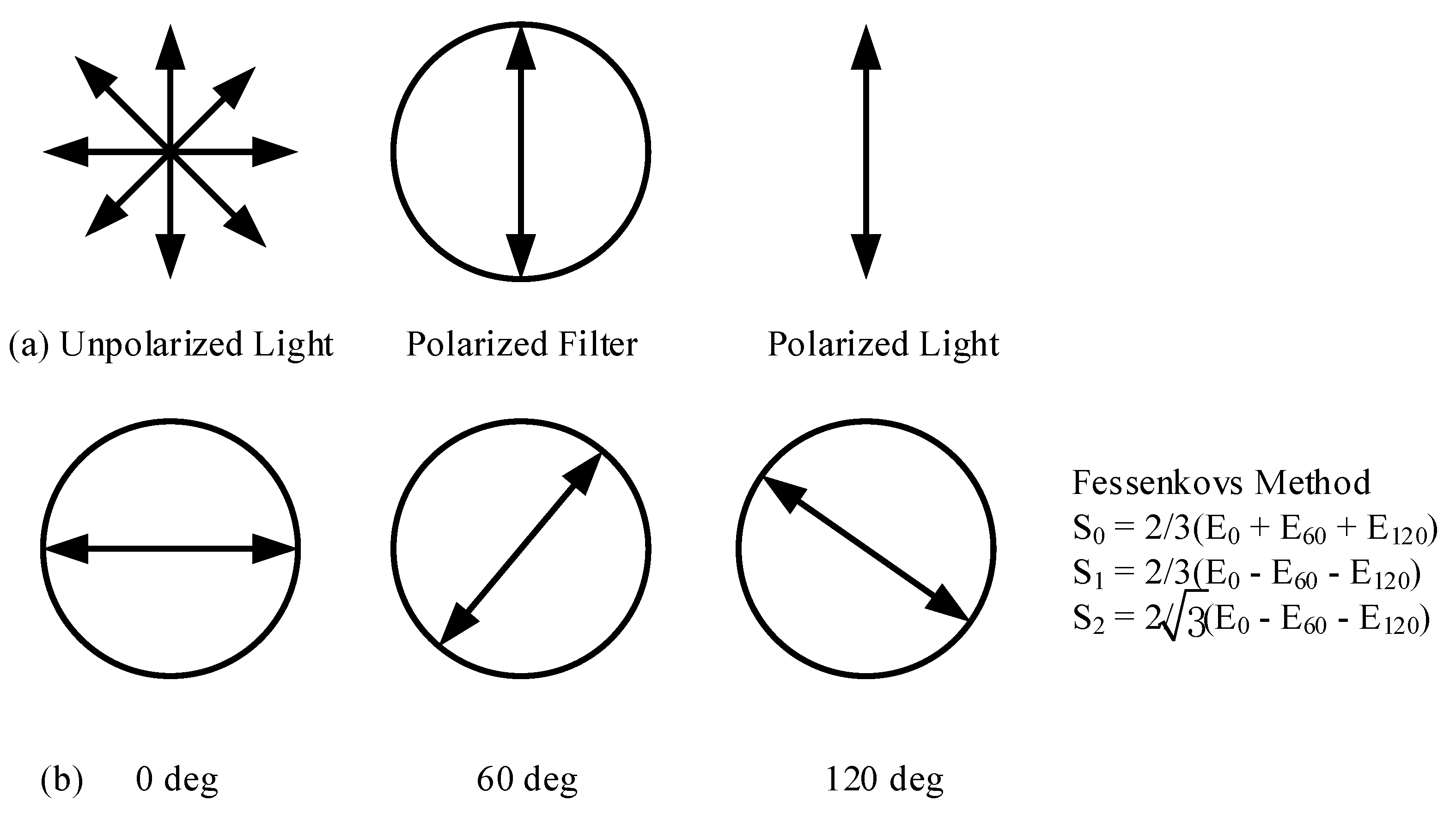
Intensity of radiation: S0 is obtained by passing light waves through linear polarizers oriented at 0 degrees, S1 is obtained by passing light waves through linear polarizers oriented at 60 degrees, and S2 is obtained by passing light waves through linear polarizers oriented at 120 degrees.
The method for measuring linear Stokes parameters is shown in Figure 3 [64]. It should be noted that, in remote sensing measurements, the degree of circular polarization is usually very small, so we only describe the linear polarization state of the beam.
Fessenkovs method was used to measure the Stokes parameters in the paper.
Degree of Linear Polarization (DoLP):
Angle of Polarization (AOP):
2.4.3. Fusion Algorithm for Nighttime Plant Detection
In view of the different polarization and spectral characteristics of healthy and stressed vegetation, in this paper, we propose a fusion algorithm to detect the vegetation with the spectral and polarization characteristics of diffuse and specular reflections of vegetation. The NDVI, DoLP and AOP are all calculated in the fusion algorithm to better detect the health status of plants in the night environment.
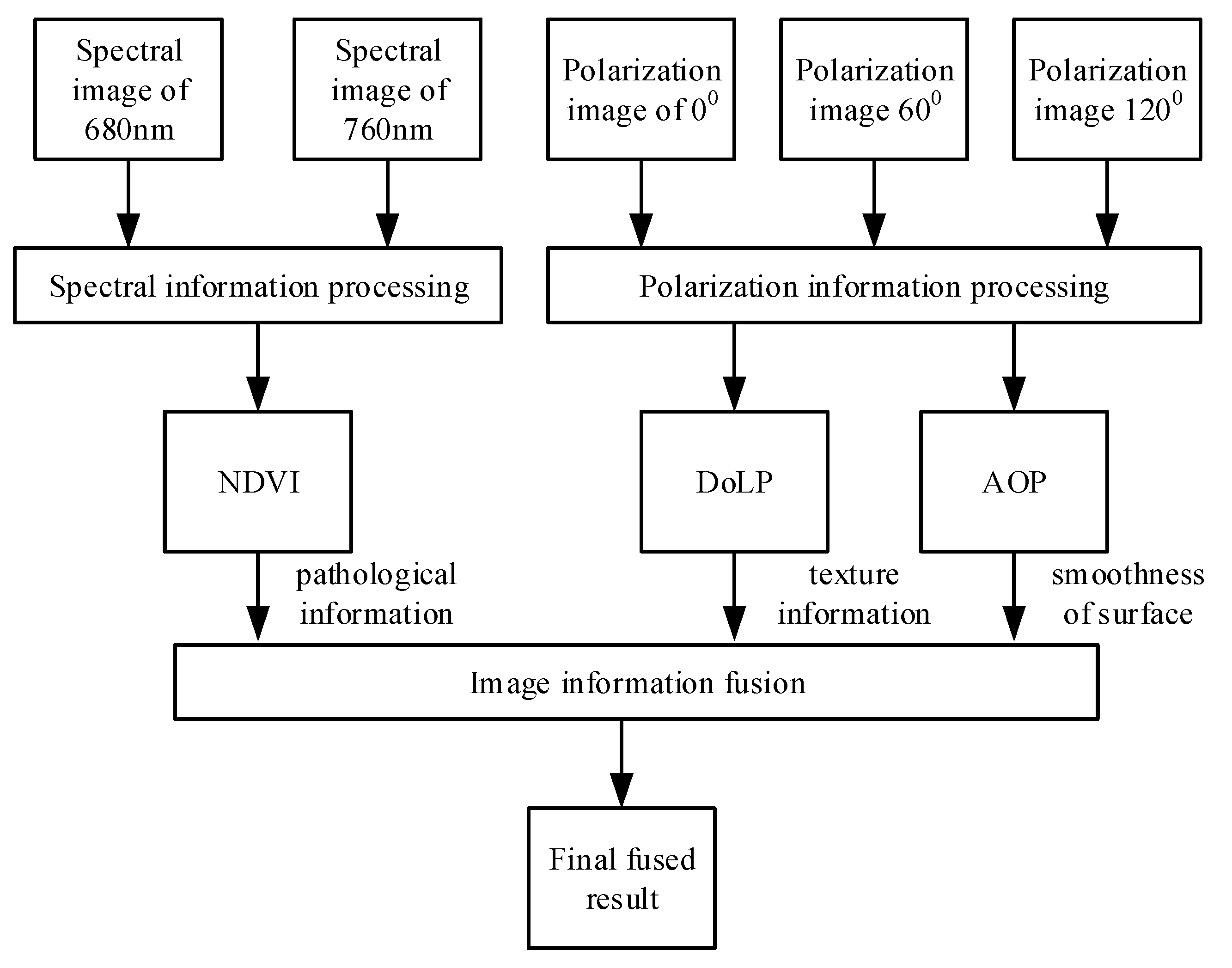
The schematic diagram of our method is shown in Figure 4. This algorithm can be summarized as follows: (1) Spectral and polarized images are preprocessed (normalization and filtering) and then co-registered together. (2) The NDVI was calculated with a F680-nm red spectral image and F760-nm infrared spectral image (Equation (1)). (3) The DoLP (Equation (3)) and AOP (Equation (4)) were calculated with 0, 60 and 120° polarized images. (4) The NDVI, DoLP and AOP images were fused, and the fused images were converted into HSV with RGB color mapping.
The images are combined following the conversion from HSV to RGB color maps:
Based on the fusion image (NDAI) of the NDVI, DoLP and AOP, a new index, the night plant state detection index (NPSDI), was proposed.
The NPSDI formula (Equation (1)) is as follows:
R(AOP), G(NDAI) and B(DoLP) represent the intensity values of the R, G and B channels of the fused image, respectively.
3. Results
3.1. Experiments on Different Illumination of Vegetation
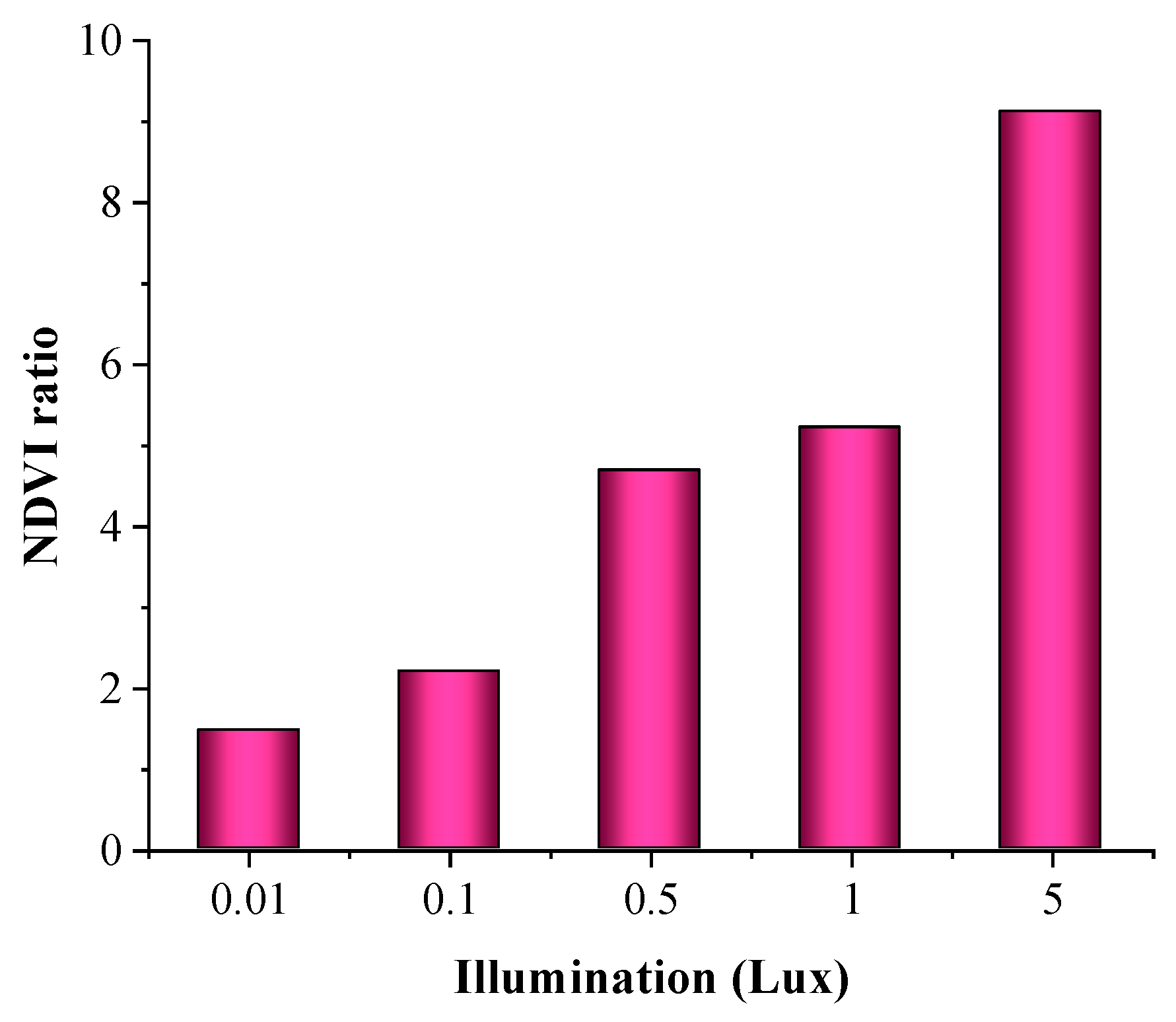
Five groups of illuminance experiments were carried out: 0.01, 0.1, 0.5, 1 and 5 lux, and spectral data were collected to calculate the NDVI. Figure 5 shows the NDVI under different illuminances. The corresponding illuminances are 0.01 (Figure 5a), 0.1 (Figure 5b), 0.5 (Figure 5c), 1.0 (Figure 5d) and 5.0 lux (Figure 5e).
As shown in Figure 5f1, some regions of interest in Figure 5b–f were selected. Fifty-one pixels were selected from the black and white regions, respectively, averaged and then divided. Then, as shown in Figure 6, the NDVI changes with the illumination. It can be clearly seen from Figure 6 that the NDVI changes significantly with the increase of the illumination. Therefore, the NDVI is greatly affected by the illuminance of the experimental environment, so it is not reliable to use the NDVI to monitor the vegetation state at night, and it should be supplemented and corrected with other information.
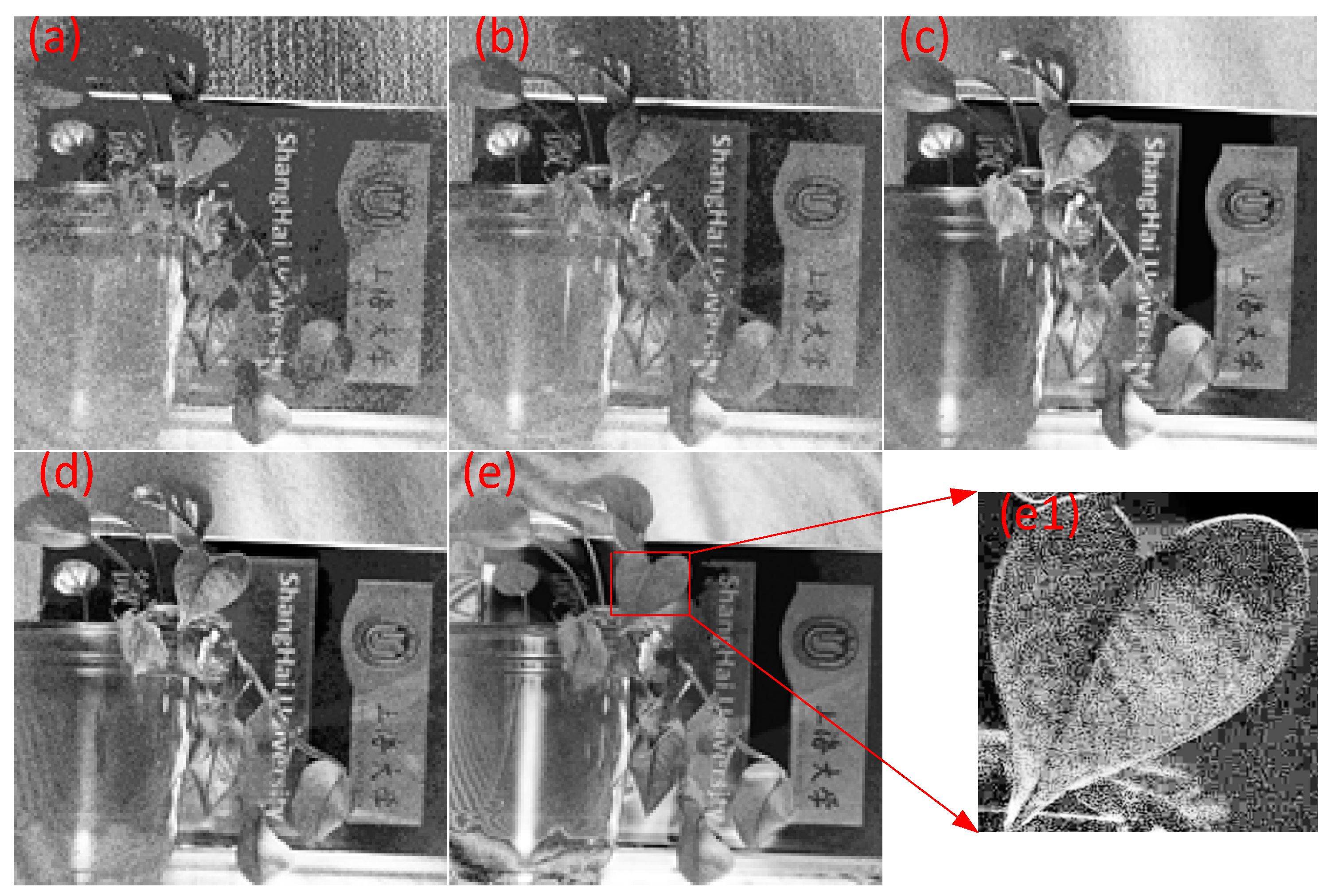
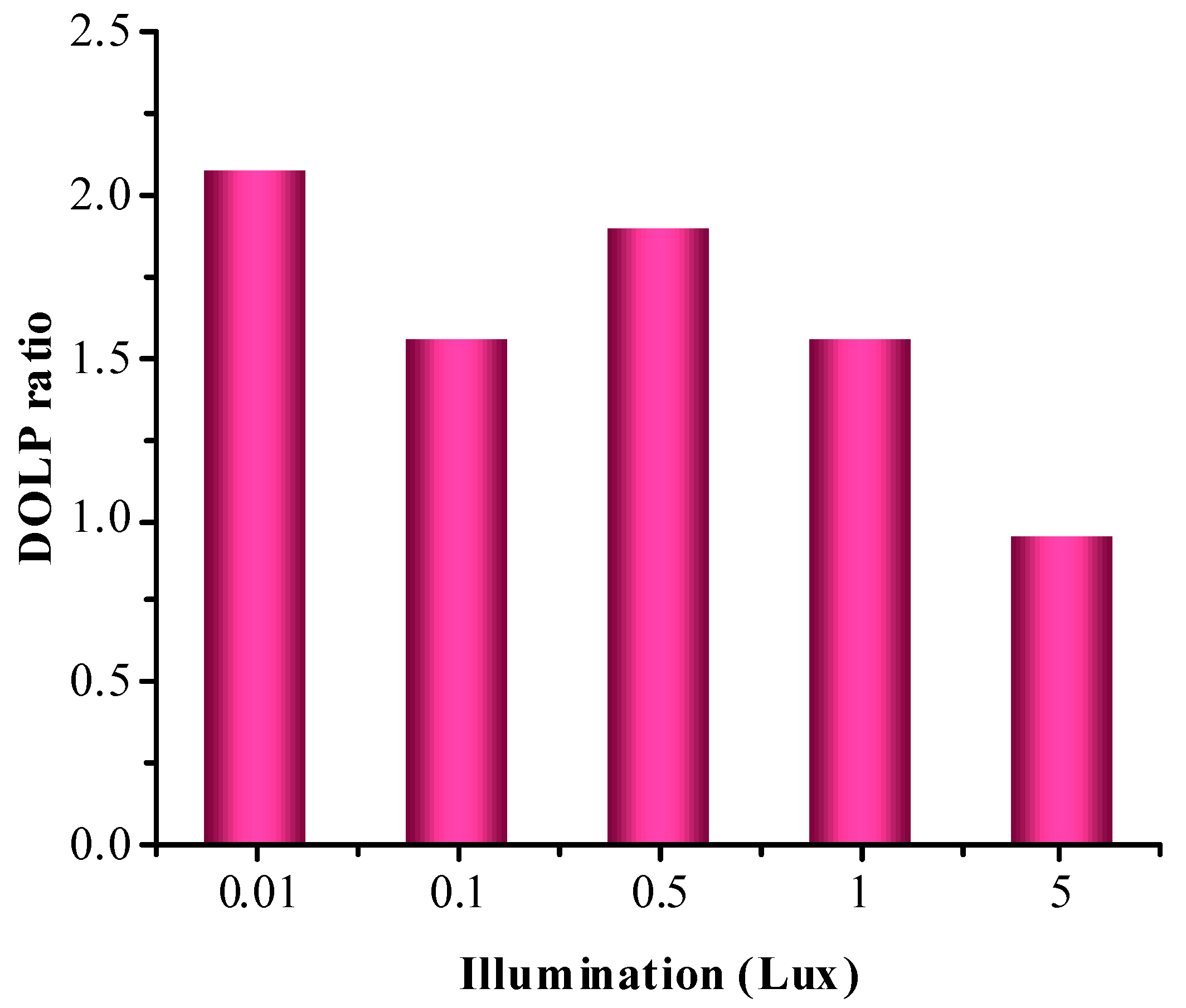
Figure 7a–e is the calculated linear polarization (DoLP) images under illuminations of 0.01, 0.1, 0.5, 1.0 and 5.0 lux, respectively. Some regions of interest in Figure 7a–e are selected, as shown in Figure 7e1, and 51 pixels are selected for the black and white regions in Figure 7e1, averaged and then divided. Then, as shown in Figure 8, the image of the DoLP changes with the illumination. It can be clearly seen from Figure 8 that the DoLP of vegetation does not change significantly with the increase of illumination. Thus, the DoLP was almost insensitive to ambient illumination. It can be seen from Figure 7 that the polarization imaging shows detailed information of the foliage, so the use of the DoLP for monitoring the nighttime vegetation state can be used to supplement the information for NDVI monitoring.
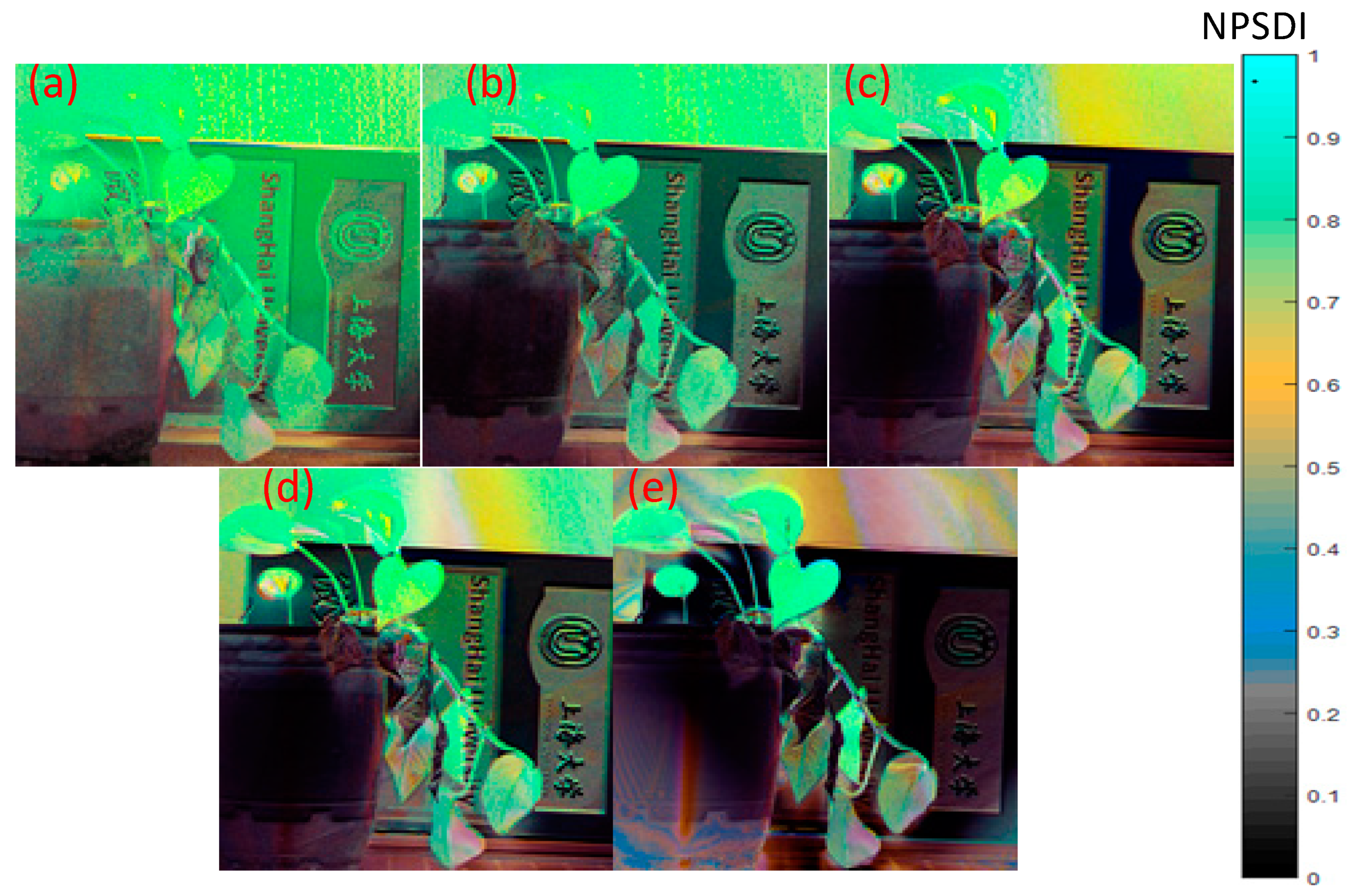
Figure 9a–e is the fusion images (NDAI) calculated by the NDVI, DoLP and AOP, and the illuminance is 0.01, 0.1, 0.5, 1.0 and 5.0 lux, respectively. The results show that healthy and nonhealthy vegetation can be well-distinguished from each other. The fusion images (NDAI) highlight more detailed information of the leaf surface than the NDVI image, and the contrast by target monitoring is enhanced.
3.2. Time Series Experiment of Vegetation
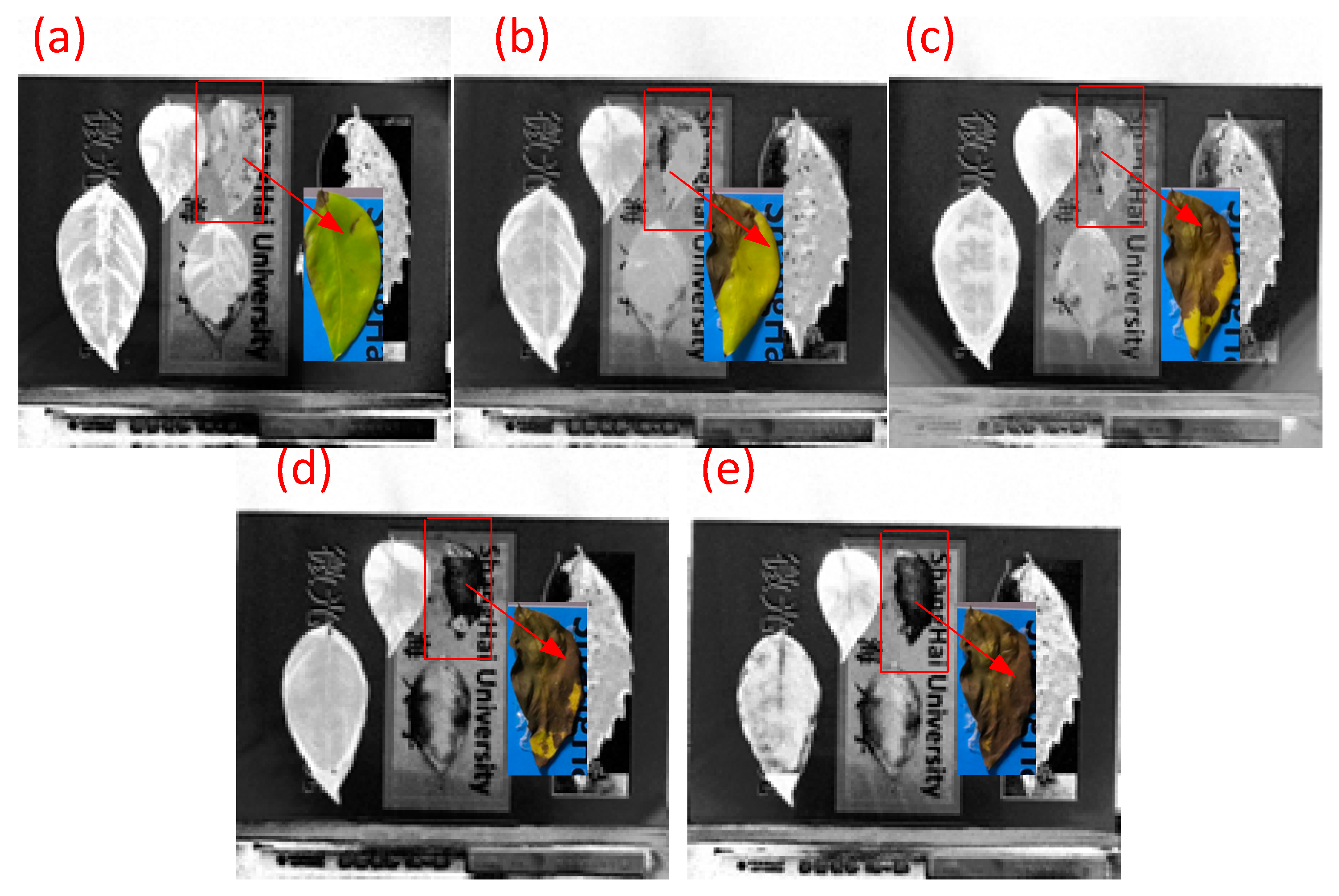
During the experiments, measurements were made once every 3 days, and five groups of experiments were carried out, respectively. Spectral data of the leaves were collected to calculate the NDVI. Figure 10 shows the NDVI time series picture, in which the red arrow refers to the corresponding color picture, and the illumination is 0.5 lux.
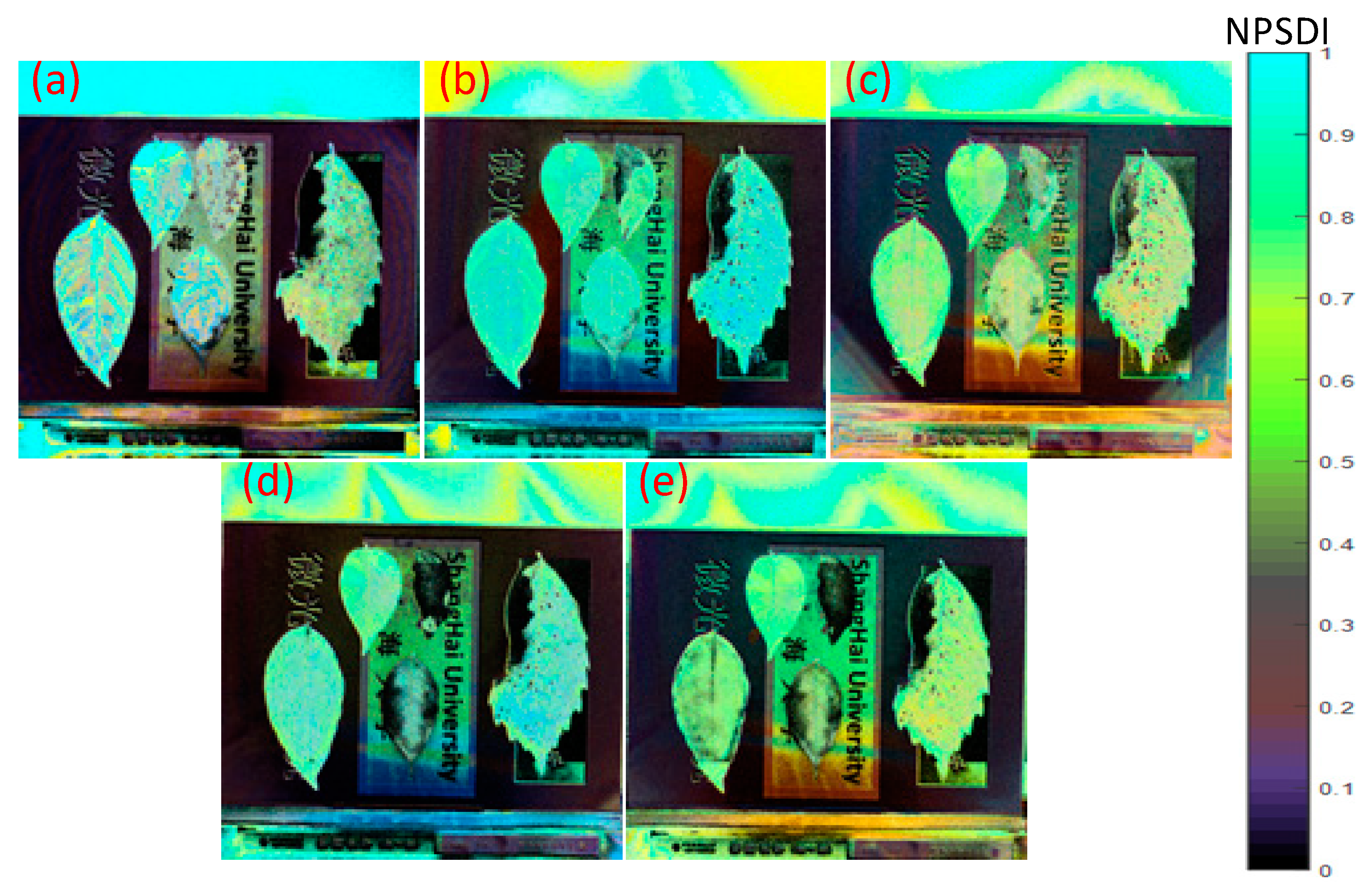
Figure 11a–e is a fusion image (NDAI) calculated from the NDVI, DoLP and AOP. It can be seen that the fusion image can track the information of the changes in the leaf health status.
3.3. Outdoor Experiment at Night
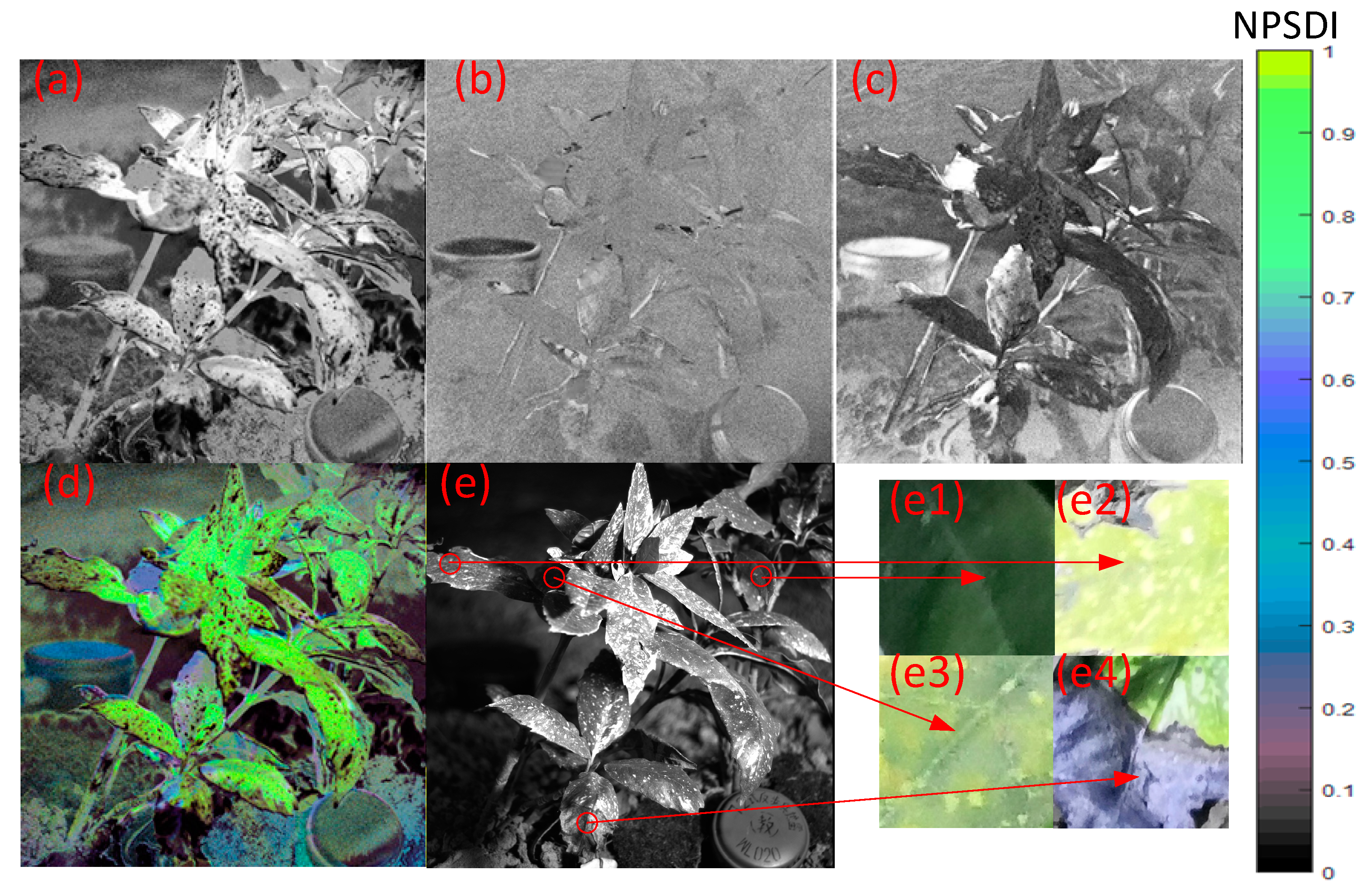
The developed polarized multispectral for a low-illumination-level imaging system was used in outdoor experiments, and as measured by the illuminator, the ambient illumination was 0.22 lux. As shown in the figure below, Figure 12a is the NDVI image calculated by Formula (1), Figure 12b the AOP image by Formula (4), Figure 12c the DoLP image by Formula (3), Figure 12d the NDAI image by Formula (5) and Figure 12e the gray-scale image. Figure 12e1–e4 are four different health state regions of plants, respectively.
The spectral image, polarization image and fusion image (NDAI) were obtained through PMSIS. Four regions: healthy leaf region (Figure 12e1), level-2 stress leaf region (Figure 12e2), level-1 stress leaf region (Figure 12e3) and withered leaf region (Figure 12e4) were selected to draw the scatter graph of the discriminant function.
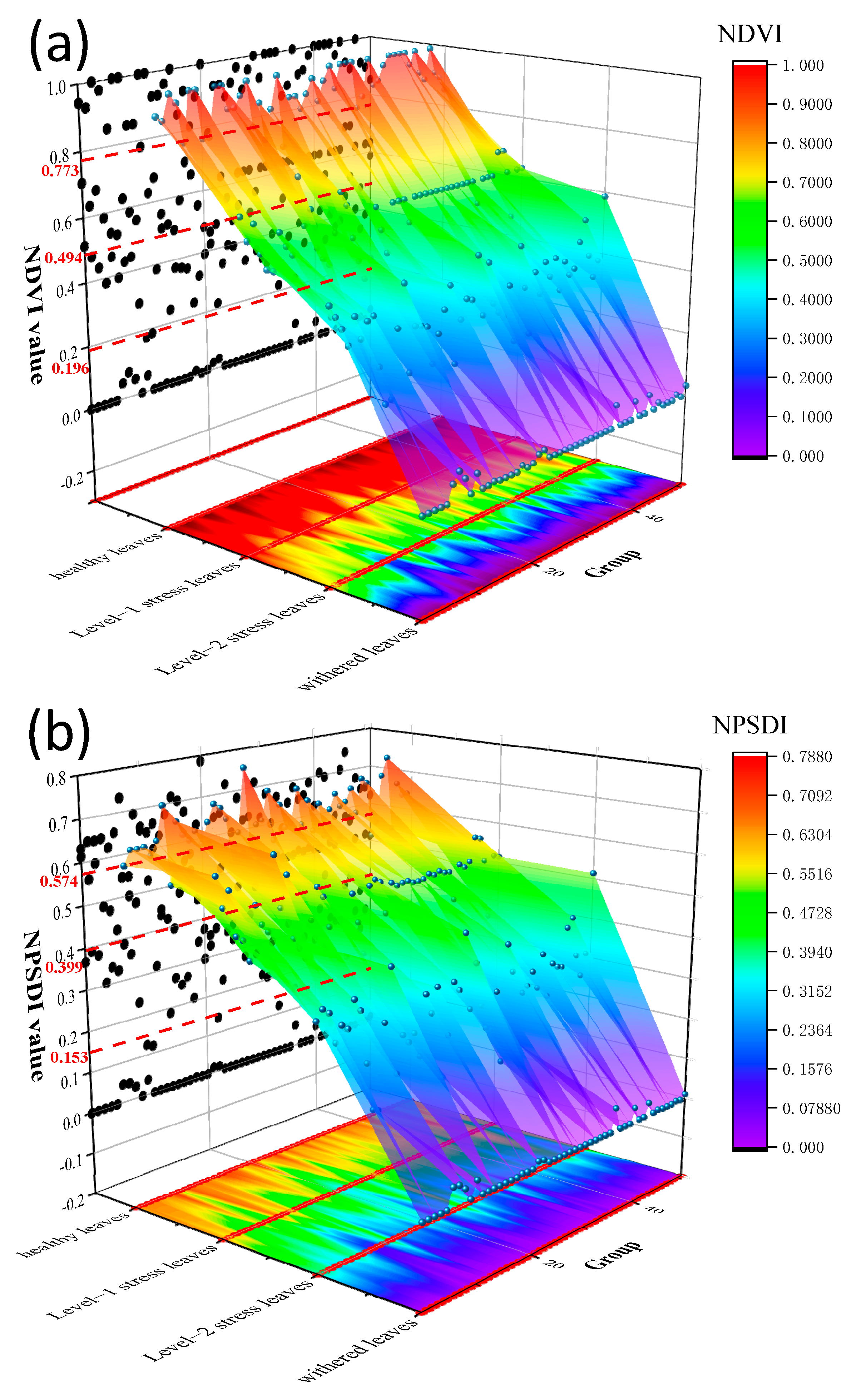
Figure 13a shows the 3D scatter plot of the NDVI image obtained from the F680 nm and F760 nm bands of the selected location points in a specific region, in which the X-axis stands for the health status level of vegetation, the Y-axis the number of groups and the Z-axis the NDVI value. The change trend of vegetation health can be seen intuitively through the change of color and trend of the curved surface. The curved surface is projected on the XY plane and the YZ plane. The cut-off lines are drawn from the arithmetic mean value of the status grades of adjacent vegetation on the YZ plane. For example, a cut-off line with a value of 0.196 distinguished a withered leaf from a level-2 stressed leaf, one with a value of 0.494 distinguished a level-1 stressed leaf from a level-2 stressed leaf and one with a value of 0.773 of distinguished a healthy leaf from a level-1 stressed leaf. According to the misclassification rate of the adjacent plant states, the sensitivity and specificity of the classification of different plant health states were determined, and the positive predictive value (PPV) and negative predictive value (NPV) of the classification are shown in Table 1.
According to the NDVI, DoLP and AOP image data, the image fusion was carried out, and the 3D scatter plot of the NPSDI was made in the selected four feature regions; the X-axis stands for the health status level of vegetation, the Y-axis the number of groups and the Z-axis the NPSDI value, as shown in Figure 13b. In the YZ plane, the cut-off line between a withered leaf and level-2 stressed leaf laid at 0.153 and that between a level-1 stressed leaf and level-2 stressed leaf and that between a healthy leaf and level-1 stressed leaf laid at 0.399 and 0.574, respectively. Table 1 also contains the sensitivity and specificity for classifying different levels of the plant health status according to the scatter plot shown in Figure 13b, as well as the corresponding PPV and NPV.
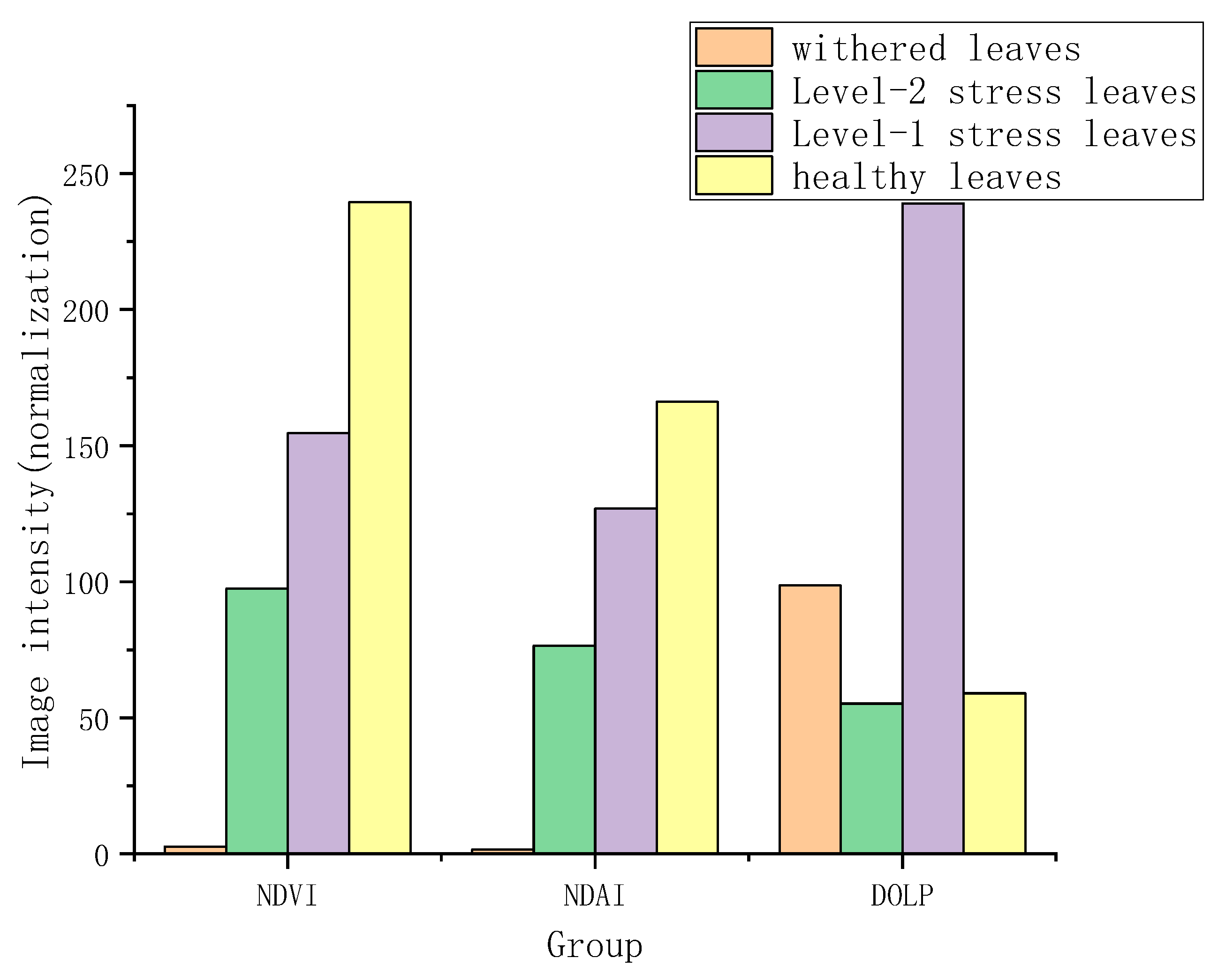
In the four plant health state regions, 51 pixels were selected and averaged to draw the NDVI, NPSDI and DoLP histogram of the four regions. As shown in Figure 14, the NDVI values show an increasing trend with the improvement of the plant health status, and the NPSDI values show the same trend. This also indicates that there is a correlation between the NDVI and NPSDI.
The reason for the higher value of the DoLP in the level-1 stress leaf region may lie in that it is also the leaf shadow region. Since the target was inversely proportional to the DoLP and surface reflectance [65], the DoLP of the shadow area is higher, which is helpful for monitoring the shadow area. The value of the DoLP in the withered leaf region was higher than that in the healthy leaf region. The reason may lie in that the completely withered leaves with more diffuse reflections lead to a higher DoLP value. Under low night illumination, the healthy leaves are smooth, but the mirror reflection is low, so the DoLP value is lower.
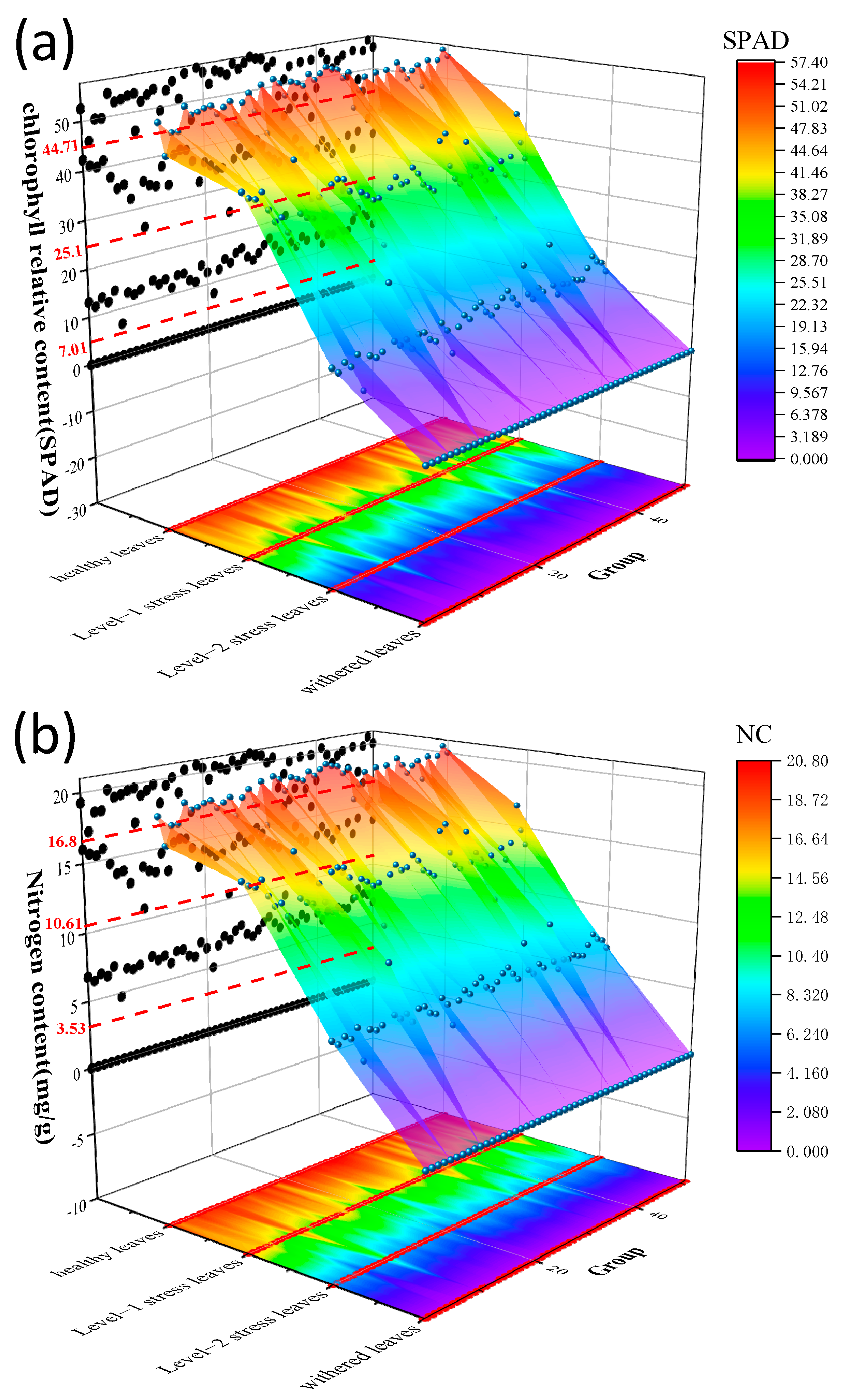
The NC and SPAD were measured for spotted laurel with leaves at varying levels of health status. It was observed that the NC of healthy leaves was above 16.8 mg/g, and it decreased to a value between 10.61 and 16.8 mg/g for level-1 stress leaves. The NC of level-2 stress leaves was in the range of 3.53–10.61 mg/g and that of withered leaves was below 3.53 mg/g. In comparison, the SPAD content of healthy leaves was above 44.71, that of level-1 stress leaves in the range of 25.22–44.71, that of level-2 stress leaves in the range of 7.01–25.22 and that of withered leaves below 7.01. The three-dimensional scatter plots of the NC and SPAD contents in the leaves of different health states are shown in Figure 15a,b. The sensitivity and specificity of using the NC and SPAD to distinguish different levels of the plant health status, as well as the respective PPV and NPV values, are shown in Table 1.
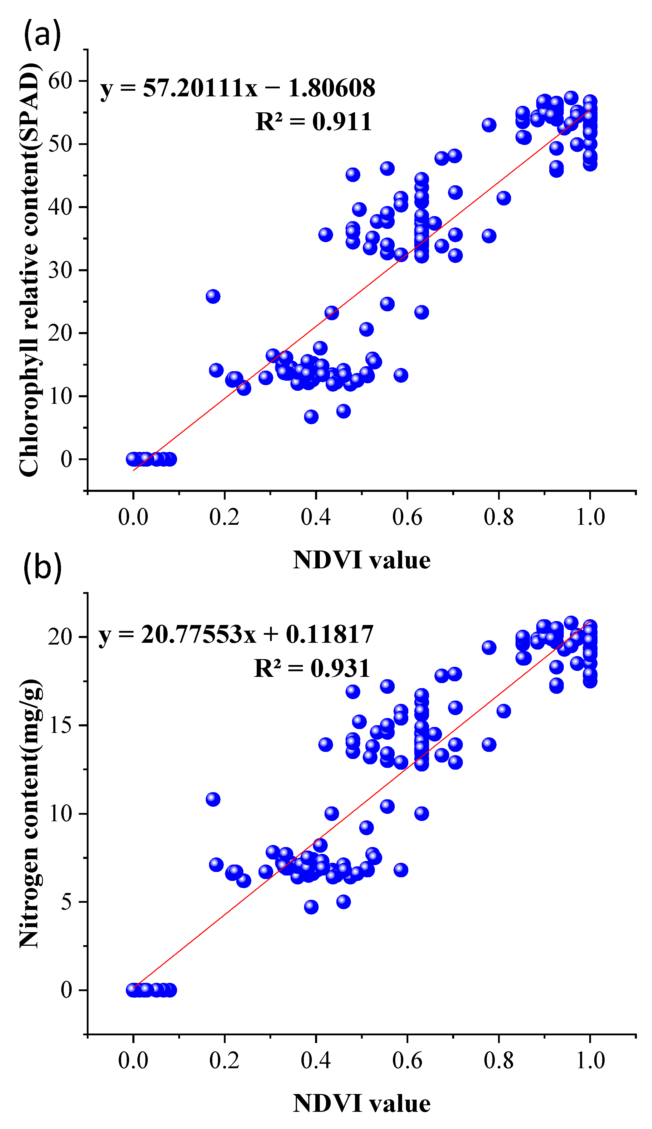
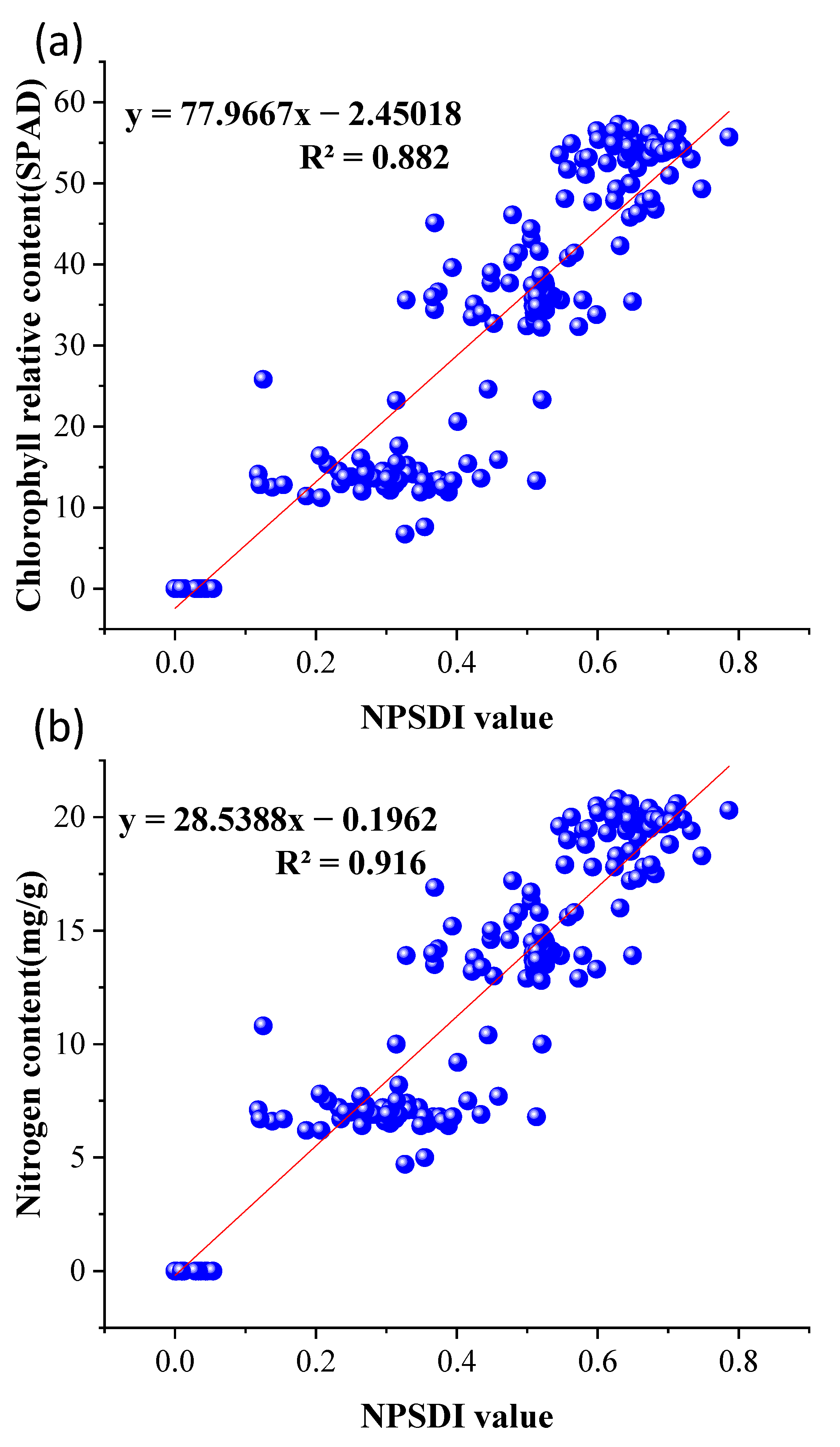
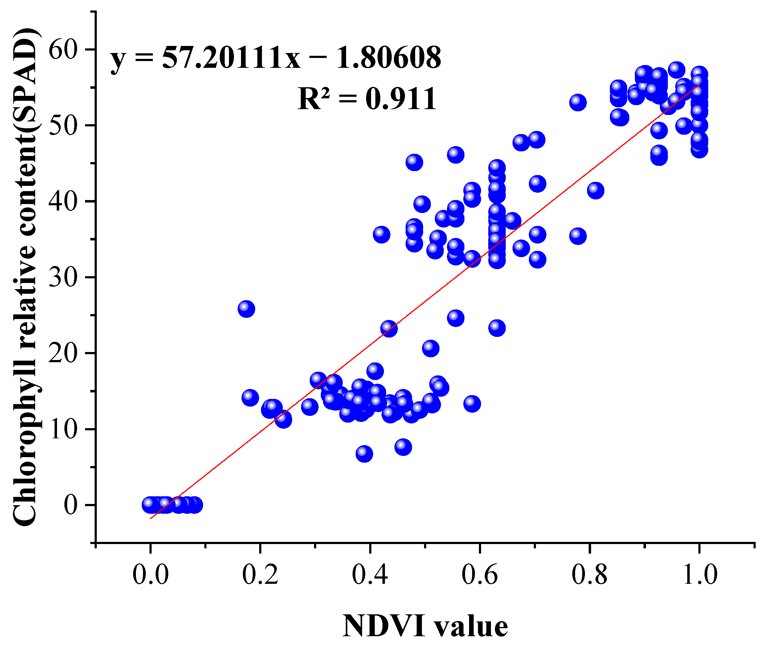
The NDVI image obtained through PMSIS system imaging and the calculated fusion image (NDAI) have a significant positive linear correlation with the NC and SPAD, and so do the NDVI and NPSDI (Figure 16a,b and Figure 17a,b). The results of the different health states showed that the correlation coefficient between the NC and NDVI was the highest (R2 = 0.931) and that of the SPAD under the same NDVI was 0.911. In comparison, the R2 values of the NPSDI with the SPAD and NC of the plant leaves were 0.882 and 0.916, respectively.
The relationship between the NDVI and NPSDI obtained using PMSIS was studied under different health states of plants, separately. As seen from Figure 18, there is a positive linear relationship between the NDVI and NPSDI (R2 = 0.968), which can be used to evaluate stress-induced changes in plants.
4. Discussion
A polarized multispectral for low-illumination-level imaging system was developed to monitor the plant status at night and evaluate stress-induced plant changes. The reflectance images of leaves on 680-nm and 760-nm narrow spectral lines were recorded by spectral technology, and the 0°, 60° and 120° polarization images of vegetation were recorded by polarization technology. The NDVI, DoLP and AOP images of vegetation were calculated by Formulas (1), (3) and (4), respectively. Then, the NDVI, DoLP and AOP images were fused by Formula (5). For example, a DOLP image can reflect the smoothness and rich texture information of the leaf surface, an AOP image can reflect the smoothness of the leaf surface and a NDVI image contains the pathological information of vegetation. Therefore, if the NDVI, DOLP and AOP images are fused, the generated images will carry more abundant vegetation information.
The research on remote sensing of the vegetation health status based on the vegetation index has become a main research approach for scholars. However, for the study of the health status of vegetation at night, the vegetation index is greatly affected by the illumination [66,67,68]. As shown in Figure 6, the NDVI value decreases with the decrease of the environmental illumination. Therefore, it is not reliable to only use the NDVI as an indicator of the plant stress degree in a low illumination environment at night.
It can be seen clearly in Figure 8 that, with the increase of illumination, there is no significant change in the DoLP of vegetation. Therefore, the DoLP is hardly affected by the illumination of the experimental environment. In addition, polarized images have the potential to provide additional information about the target’s shape, shadow, roughness and surface characteristics [69,70]. There are relatively few studies on polarization technology providing contrast enhancement information for the detection of vegetation health. Therefore, in this paper, we proposed the fusion of the vegetation index (NDVI), DoLP and AOP to better detect the physiological state of plants in a nighttime environment. As shown in Figure 9, Figure 11 and Figure 12d, different health states of plants correspond to different colors, so the proposed enhancement algorithm for nighttime plant detection has the effect of enhancing the contrast.
Under stress, the decrease of the NDVI ratio was related to the decrease of the SPAD content, and this proportional relationship could be explained by the optical characteristics of leaves. Compared with healthy leaves, those under stress had lower chlorophyll contents [71], and the reduced chlorophyll content led to a decreased chlorophyll absorption and enhanced reflectance at F680 nm. Moreover, the reflectance at F760 nm was reduced. According to Formula (1), the NDVI ratio was bound to decrease. In the NDVI images, the NDVI ratio of the stressed leaves was low (Figure 12a). Due to the fusion of polarization, the contrast of the fused images was enhanced, and leaf lesions could be identified more clearly (Figure 12d). It can be pointed out that the increase of the stress degree will lead to a lower vegetation index and leaf chlorosis [72,73].
Three-dimensional scatter plots (Figure 13a,b) were drawn using NDVI and NPSDI data obtained from the polarized multispectral low-light-level imaging monitoring system to classify different health status levels of plants. The classification discrimination accuracy is shown in Table 1. It can be seen from Table 1 that the sensitivity and specificity of the fusion image for the classification of different plant health conditions are generally close to the NDVI image data. It is important that the fusion image shows a color contrast, and the fusion image carries richer object information, so it is excellent to use the proposed fusion image algorithm to monitor the health of plants. In addition, the sensitivity and specificity of the fusion image (NDAI) to classify healthy leaves from stress level-1 were 89% and 92%, which was significant, as they demonstrate the potential of the fusion algorithm for detecting early symptoms of stressed plants at night.
The decrease of the chlorophyll and nitrogen contents under stress was also consistent with previous studies. We believe that the decrease of the chlorophyll content in stressed leaves may be caused by the degradation of chloroplasts in stressed leaves [74,75]. The scatter plots of the chlorophyll and nitrogen contents (Figure 15a,b) were similar to those of the NDVI and NPSDI and tended to decrease with the increase of the leaf stress degree. By drawing the distinguishing lines of different stress levels, the diagnostic accuracy of different stress levels can be determined (Table 1). It can be seen that the NDVI and NPSDI have similar diagnostic accuracies in distinguishing different levels of stress, while the SPAD has a higher correlation with stress and higher diagnostic accuracy. Furthermore, the NDVI determined through a spectra analysis follows a linear relationship with the SPAD and NC (Figure 16a,b), and the NPSDI obtained through a fusion algorithm for nighttime plant detection follows a linear relationship with the SPAD and NC (Figure 17a,b). There was also a linear correlation between the NDVI and NPSDI (Figure 18), which shows the potential of applying the fusion image determined by PMSIS in understanding the health status of outdoor plants at night from proximal sensing platforms.
In contrast to point monitoring devices such as spectroradiometers and hand-held chlorophyll analyzers, imaging devices provide spatial distribution information on the properties of the objects being detected. The advantage of PMSIS imaging is that it is a passive technology. It is a relatively inexpensive and compact instrument that can be easily carried anywhere and deployed on platforms (such as cars and drones) to feel the effects of various types of stress on farmlands and forests at night.
5. Conclusions
We built a polarized multispectral for a low-illumination-level imaging system and a polarized multispectral low-light imaging system (PMSIS), incorporating a SCOMS camera, rotating filter wheel and linear polarizer, for monitoring the health status of plants outdoors at night. With a compact size, the developed system is portable, consisting of a minimum number of moving parts, which makes it ideal for field measurements. We have done some research on the potential of polarization technology to provide contrast enhancement information for vegetation assessments. Polarization imaging and multispectral imaging can provide complementary discrimination information for target monitoring and other applications. However, few people have proposed to fuse the information of polarized images and multispectral images to obtain better target monitoring results. Therefore, a fusion algorithm based on the spectral and polarization characteristics of the diffuse and specular reflection of vegetation is proposed to detect vegetation at night. The NDVI, DoLP and AOP were all computed within a fusion framework to better monitor the health status of plants in a nighttime environment.
In order to evaluate the remote sensing power of the fusion algorithm in monitoring the plant health status at night, the leaf regions of spotted laurel in different health states were measured. The changes of the SPAD, NC, NDVI and NPSDI in different health levels of plants were determined, and the health degrees of spotted laurel were classified. The value of the NPSDI decreased with the decrease of the plant health status, and it was in a positive linear correlation with the physiological parameters such as the SPAD and NC. The correlation of the NPSDI with NC was 0.916, while, with the SPAD, it was 0.882. In applying the fusion algorithm in classifying healthy leaves from level-1 stress leaves, the sensitivity obtained was 89% and the specificity 92%, which suggests the effectiveness of the method for the early detection of the health status in field-grown plants.
In this paper, the fusion of the NDVI, DoLP and AOP was proposed for the first time. The proposed fusion algorithm enhanced the contrast effect, and the resultant image carried more abundant information of the object; thus, monitoring the health status of plants at night becomes more effective. The fusion algorithm makes up for the unreliability of the NDVI in a low-illumination environment. Based on the polarimetric imaging system that we developed, polarization information improved the monitoring accuracy at night with traditional NDVI information. In the study of monitoring the plant health status at night, we found that the NPSDI was excellent in tracking stress-induced plant changes. The NPSDI scatter plots were used to study for classifying different grades of the health state in spotted laurel, and the sensitivity and specificity were good, which indicated that this technique was suitable for the classification of the outdoor plant health status and various stresses. This study provided the basis for the promotion and use of PMSIS from various remote sensing platforms (such as cars and drones) to assess the crop health status by polarization spectral imaging at night. In the future, the system can be improved (a three-camera real-time imaging system), so that it can be installed on vehicle and airborne devices, enabling its application in a large area for monitoring the health of vegetation at night. The system has the following applications: (1) the detection of the vegetation status in low-illumination environments, (2) the detection of the vegetation status during the day, (3) the detection of the polarization of vegetation leaves and (4) the detection of artificial targets in vegetation environments.
We supplement a table at the end of paper. Acronyms are shown in Table 2.
Author Contributions
J.J. and C.W. conceived and designed the experiments; S.L. performed the experiments and analyzed and interpreted the results. All authors have read and agreed to the published version of the manuscript.
Funding
This research was funded by the National Natural Science Foundation of China (No. 61773249) and Shanghai Science and Technology Innovation Action Plan (No. 20142200100) for project funding.
Acknowledgments
Thanks to the colleagues and students who participated in the outdoor data collection.
Conflicts of Interest
The authors declare no conflict of interest.
References
- Food and Agriculture Organization of the United Nations. The State of the World’s Forests 2018—Forest Pathways to Sustainable Development; Food and Agriculture Organization of the United Nations: Rome, Italy, 2018. [Google Scholar]
- Zhou, Y.; Wu, L.; Zhang, H.; Wu, K. Spread of invasive migratory pest spodoptera frugiperda and management practices throughout china. J. Integr. Agric. 2021, 20, 637–645. [Google Scholar] [CrossRef]
- Tong, A.; He, Y. Estimating and mapping chlorophyll content for a heterogeneous grassland: Comparing prediction power of a suite of vegetation indices across scales between years. ISPRS J. Photogramm. Remote Sens. 2017, 126, 146–167. [Google Scholar] [CrossRef]
- Sharma, R.C.; Kajiwara, K.; Honda, Y. Estimation of forest canopy structural parameters using kernel-driven bi-directional reflectance model based multi-angular vegetation indices. ISPRS J. Photogramm. Remote Sens. 2013, 78, 50–57. [Google Scholar] [CrossRef]
- Yue, J.; Yang, G.; Tian, Q.; Feng, H.; Xu, K.; Zhou, C. Estimate of winter-wheat above-ground biomass based on UAV ultrahigh- ground-resolution image textures and vegetation indices. ISPRS J. Photogramm. Remote Sens. 2019, 150, 226–244. [Google Scholar] [CrossRef]
- Gao, L.; Wang, X.; Johnson, B.A.; Tian, Q.; Wang, Y.; Verrelst, J.; Mu, X.; Gu, X. Remote sensing algorithms for estimation of fractional vegetation cover using pure vegetation index values: A review. ISPRS J. Photogramm. Remote Sens. 2020, 159, 364–377. [Google Scholar] [CrossRef]
- Zhou, X.; Zheng, H.; Xu, X.; He, J.; Ge, X.; Yao, X.; Cheng, T.; Zhu, Y.; Cao, W.; Tian, Y. Predicting grain yield in rice using multi-temporal vegetation indices from UAV-based multispectral and digital imagery. ISPRS J. Photogramm. Remote Sens. 2017, 130, 246–255. [Google Scholar] [CrossRef]
- Bajgain, R.; Xiao, X.; Wagle, P.; Basara, J.; Zhou, Y. Sensitivity analysis of vegetation indices to drought over two tallgrass prairie sites. ISPRS J. Photogramm. Remote Sens. 2015, 108, 151–160. [Google Scholar] [CrossRef]
- Barbosa, H.A.; Kumar, T.L.; Paredes, F.; Elliott, S.; Ayuga, J.G. Assessment of Caatinga response to drought using Meteosat-SEVIRI Normalized Difference Vegetation Index (2008–2016). ISPRS J. Photogramm. Remote Sens. 2019, 148, 235–252. [Google Scholar] [CrossRef]
- Sakamoto, T.; Shibayama, M.; Kimura, A.; Takada, E. Assessment of digital camera-derived vegetation indices in quantitative monitoring of seasonal rice growth. ISPRS J. Photogramm. Remote Sens. 2011, 66, 872–882. [Google Scholar] [CrossRef]
- Rahimzadeh-Bajgiran, P.; Omasa, K.; Shimizu, Y. Comparative evaluation of the Vegetation Dryness Index (VDI), the Temperature Vegetation Dryness Index (TVDI) and the improved TVDI (iTVDI) for water stress detection in semi-arid regions of Iran. ISPRS J. Photogramm. Remote Sens. 2012, 68, 1–12. [Google Scholar] [CrossRef]
- Adam, E.; Deng, H.; Odindi, J.; Abdel-Rahman, E.M.; Mutanga, O. Detecting the early stage of phaeosphaeria leaf spot infestations in maize crop using in situ hyperspectral data and guided regularized random forest algorithm. J. Spectrosc. 2017, 8, 6961387. [Google Scholar] [CrossRef]
- Apan, A.; Datt, B.; Kelly, R. Detection of pests and diseases in vegetable crops using hyperspectral sensing: A comparison of reflectance data for different sets of symptoms. In Proceedings of the 2005 Spatial Sciences Institute Biennial Conference 2005: Spatial Intelligence, Innovation and Praxis (SSC2005), Melbourne, Australia, 12–16 September 2005; pp. 10–18. [Google Scholar]
- Dhau, I.; Adam, E.; Mutanga, O.; Ayisi, K.K. Detecting the severity of maize streak virus infestations in maize crop using in situ hyperspectral data. Trans. R. Soc. S. Afr. 2018, 73, 1–8. [Google Scholar] [CrossRef]
- Iordache, M.; Mantas, V.; Baltazar, E.; Pauly, K.; Lewyckyj, N. A machine learning approach to detecting pine wilt disease using airborne spectral imagery. Remote Sens. 2020, 12, 2280. [Google Scholar] [CrossRef]
- Jo, M.H.; Kim, J.B.; Oh, J.S.; Lee, K.J. Extraction method of damaged area by pinetree pest (Bursaphelenchus Xylophilus) using high resolution IKONOS image. J. Korean Assoc. Geogr. Inform. Stud. 2001, 4, 72–78. [Google Scholar]
- Mota, M.M.; Vieira, P. Pine wilt disease: A worldwide threat to forest ecosystems. Nematology 2009, 11, 5–14. [Google Scholar]
- Nguyen, V.T.; Park, Y.S.; Jeoung, C.S.; Choi, W.I.; Kim, Y.K.; Jung, I.H.; Shigesada, N.; Kawasaki, K.; Takasu, F.; Chon, T.S. Spatially explicit model applied to pine wilt disease dispersal based on host plant infestation. Ecol. Model. 2017, 353, 54–62. [Google Scholar] [CrossRef]
- Selvaraj, M.G.; Vergara, A.; Montenegro, F.; Ruiz, H.A.; Safari, N.; Raymaekers, D.; Ocimati, W.; Ntamwira, J.; Tits, L.; Bonaventure, A.; et al. Detection of banana plants and their major diseases through aerial images and machine learning methods: A case study in DR Congo and Republic of Benin. ISPRS J. Photogramm. Remote Sens. 2020, 169, 110–124. [Google Scholar] [CrossRef]
- Shi, Y.; Huang, W.; Luo, J.; Huang, L.; Zhou, X. Detection and discrimination of pests and diseases in winter wheat based on spectral indices and kernel discriminant analysis. Comput. Electron. Agric. 2017, 141, 171–180. [Google Scholar] [CrossRef]
- Son, M.H.; Lee, W.K.; Lee, S.H.; Cho, H.K.; Lee, J.H. Natural spread pattern of damaged area by pine wilt disease using geostatistical analysis. J. Korean Soc. Forest Sci. 2006, 95, 240–249. [Google Scholar]
- Baranoski, G.V.G.; Rokne, J.G. A practical approach for estimating the red edge position of plant leaf reflectance. Int. J. Remote Sens. 2005, 26, 503–521. [Google Scholar] [CrossRef]
- Rouse, J.W.; Hass, R.H.; Schell, J.A.; Deering, D.W. Monitoring vegetation systems in the great plains with ERTS. In Proceedings of the Third Earth Resources Technology Satellite-1 Symposium, Washington, DC, USA, 10–14 December 1973; Volume 1, pp. 309–317. [Google Scholar]
- Huete, A.R. A soil-adjusted vegetation index (SAVI). Remote Sens. Environ. 1988, 25, 295–309. [Google Scholar] [CrossRef]
- Qi, J.; Chehbouni, A.; Huete, A.R.; Kerr, Y.H.; Sorooshian, S. A modified adjusted vegetation index (MSAVI). Remote Sens. Environ. 1994, 48, 119–126. [Google Scholar] [CrossRef]
- Gao, B. NDWI—A normalized difference water index for remote sensing of vegetation liquid water from space. Remote Sens. Environ. 1996, 58, 257–266. [Google Scholar] [CrossRef]
- Steddom, K.; Bredehoeft, M.W.; Khan, M.; Rush, C.M. Comparison of visual and multispectral radiometric disease evaluations of cercospora leaf spot of sugar beet. Plant Dis. 2005, 89, 153–158. [Google Scholar] [CrossRef] [Green Version]
- Arens, N.; Backhaus, A.; Döll, S.; Fischer, S.; Seiffert, U.; Mock, H.P. Non-invasive presymptomatic detection of cercospora beticola infection and identification of early metabolic responses in sugar beet. Front. Plant Sci. 2016, 7, 1377. [Google Scholar] [CrossRef] [PubMed] [Green Version]
- Deery, D.; Jimenez-Berni, J.; Jones, H.; Sirault, X.; Furbank, R. Proximal remote sensing buggies and potential applications for field-based phenotyping. Agronomy 2014, 4, 349–379. [Google Scholar] [CrossRef] [Green Version]
- Vigneau, N.; Ecarnot, M.; Rabatel, G.; Roumet, P. Potential of field hyperspectral imaging as a non-destructive method to assess leaf nitrogen content in wheat. Field Crop. Res. 2011, 122, 25–31. [Google Scholar] [CrossRef] [Green Version]
- Graeff, S.; Link, J.; Claupein, W. Identification of powdery mildew (Erysiphe graminis sp. tritici) and take-all disease (Gaeumannomyces graminis sp. tritici) in wheat (Triticum aestivum L.) by means of leaf reflectance measurements. Open Life Sci. 2006, 1, 275–288. [Google Scholar] [CrossRef]
- Yang, Z.; Rao, M.N.; Elliott, N.C.; Kindler, S.D.; Popham, T.W. Differentiating stress induced by greenbugs and Russian wheat aphids in wheat using remote sensing. Comput. Electron. Agric. 2009, 67, 64–70. [Google Scholar] [CrossRef]
- Liu, Z.Y.; Wu, H.F.; Huang, J.F. Application of neural networks to discriminate fungal infection levels in rice panicles using hyperspectral reflectance and principal components analysis. Comput. Electron. Agric. 2010, 72, 99–106. [Google Scholar] [CrossRef]
- Prabhakar, M.; Prasad, Y.; Thirupathi, M.; Sreedevi, G.; Dharajothi, B.; Venkateswarlu, B. Use of ground based hyperspectral remote sensing for detection of stress in cotton caused by leafhopper (Hemiptera: Cicadellidae). Comput. Electron. Agric. 2011, 79, 189–198. [Google Scholar] [CrossRef]
- Prabhakar, M.; Prasad, Y.G.; Vennila, S.; Thirupathi, M.; Sreedevi, G.; Ramachandra Rao, G.; Venkateswarlu, B. Hyperspectral indices for assessing damage by the solenopsis mealybug (Hemiptera: Pseudococcidae) in cotton. Comput. Electron. Agric. 2013, 97, 61–70. [Google Scholar] [CrossRef]
- Nebiker, S.; Lack, N.; Abächerli, M.; Läderach, S. Light-weight multispectral UAV sensors and their capabilities for predicting grain yield and detecting plant diseases. ISPRS—International Archives of the Photogrammetry. Remote Sens. Spat. Inf. Sci. 2016, XLI-B1, 963–970. [Google Scholar]
- Dash, J.P.; Watt, M.S.; Pearse, G.D.; Heaphy, M.; Dungey, H.S. Assessing very high resolution UAV imagery for monitoring forest health during a simulated disease outbreak. ISPRS J. Photogramm. Remote Sens. 2017, 131, 1–14. [Google Scholar] [CrossRef]
- Yang, C.H.; Everitt, J.H.; Fernandez, C.J. Comparison of airborne multispectral and hyperspectral imagery for mapping cotton root rot. Biosyst. Eng. 2010, 107, 131–139. [Google Scholar] [CrossRef]
- Calderón, R.; Navas-Cortés, J.A.; Lucena, C.; Zarco-Tejada, P.J. High-resolution airborne hyperspectral and thermal imagery for early detection of Verticillium wilt of olive using fluorescence, temperature and narrow-band spectral indices. Remote Sens. Environ. 2013, 139, 231–245. [Google Scholar] [CrossRef]
- Sanches, I.; Filho, C.R.S.; Kokaly, R.F. Spectroscopic remote sensing of plant stress at leaf and canopy levels using the chlorophyll 680nm absorption feature with continuum removal. ISPRS J. Photogramm. Remote Sens. 2014, 97, 111–122. [Google Scholar] [CrossRef]
- Lehmann, J.; Nieberding, F.; Prinz, T.; Knoth, C. Analysis of Unmanned Aerial System-Based CIR Images in Forestry—A New Perspective to Monitor Pest Infestation Levels. Forests 2015, 6, 594–612. [Google Scholar] [CrossRef] [Green Version]
- Yuan, L.; Pu, R.; Zhang, J.; Wang, J.; Yang, H. Using high spatial resolution satellite imagery for mapping powdery mildew at a regional scale. Precis. Agric. 2016, 17, 332–348. [Google Scholar] [CrossRef]
- Chen, D.; Shi, Y.; Huang, W.; Zhang, J.; Wu, K. Mapping wheat rust based on high spatial resolution satellite imagery. Comput. Electron. Agric. 2018, 152, 109–116. [Google Scholar] [CrossRef]
- Zheng, Q.; Huang, W.; Cui, X.; Shi, Y.; Liu, L. New Spectral Index for Detecting Wheat Yellow Rust Using Sentinel-2 Multispectral Imagery. Sensors 2018, 18, 868. [Google Scholar] [CrossRef] [Green Version]
- Meiforth, J.J.; Buddenbaum, H.; Hill, J.; Shepherd, J.D.; Dymond, J.R. Stress Detection in New Zealand Kauri Canopies with WorldView-2 Satellite and LiDAR Data. Remote Sens. 2020, 12, 1906. [Google Scholar] [CrossRef]
- Li, X.; Yuan, W.; Dong, W. A Machine Learning Method for Predicting Vegetation Indices in China. Remote Sens. 2021, 13, 1147. [Google Scholar] [CrossRef]
- Rvachev, V.P.; Guminetskii, S.G. The structure of light beams reflected by plant leaves. J. Appl. Spectrosc. 1966, 4, 303–307. [Google Scholar] [CrossRef]
- Woolley, J.T. Reflectance and transmission of light by leaves. Plant Physiol. 1971, 47, 656–662. [Google Scholar] [CrossRef] [PubMed] [Green Version]
- Vanderbilt, V.C.; Grant, L.; Daughtry, C.S.T. Polarization of light scattered by vegetation. Proc. IEEE 1985, 73, 1012–1024. [Google Scholar] [CrossRef]
- Vanderbilt, V.C.; Grant, L.; Biehl, L.L.; Robinson, B.F. Specular, diffuse, and polarized light scattered by two wheat canopies. Appl. Opt. 1985, 24, 2408–2418. [Google Scholar] [CrossRef] [PubMed]
- Duggin, M.J.; Kinn, G.J.; Schrader, M. Enhancement of vegetation mapping using Stokes parameter images. In Proceedings of SPIE—The International Society for Optical Engineering; Society of Photo-Optical Instrumentation Engineers: Bellingham, WA, USA, 1997; Volume 3121, pp. 307–313. [Google Scholar]
- Rondeaux, G.; Herman, M. Polarization of light reflected by crop canopies. Remote Sens. Environ. 1991, 38, 63–75. [Google Scholar] [CrossRef]
- Fitch, B.W.; Walraven, R.L.; Bradley, D.E. Polarization of light reflected from grain crops during the heading growth stage. Remote Sens. Environ. 1984, 15, 263–268. [Google Scholar] [CrossRef]
- Perry, G.; Stearn, J.; Vanderbilt, V.C.; Ustin, S.L.; Diaz Barrios, M.C.; Morrissey, L.A.; Livingston, G.P.; Breon, F.-M.; Bouffies, S.; Leroy, M. Remote sensing of high-latitude wetlands using polarized wide-angle imagery. In Proceedings of SPIE—The International Society for Optical Engineering; Society of Photo-Optical Instrumentation Engineers: Bellingham, WA, USA, 1997; Volume 3121, pp. 370–381. [Google Scholar]
- Shibayama, M. Prediction of the ratio of legumes in a mixed seeding pasture by polarized reflected light. Jpn. J. Grassl. Sci. 2003, 49, 229–237. [Google Scholar]
- Vanderbilt, V.C.; Grant, L. Polarization photometer to measure bidirectional reflectance factor R (55°, 0°; 55°, 180°) of leaves. Opt. Eng. 1986, 25, 566–571. [Google Scholar] [CrossRef]
- Vanderbilt, V.C.; Grant, L.; Ustin, S.L. Polarization of Light by Vegetation; Springer: Berlin/Heidelberg, Germany, 1991; Volume 7, pp. 191–228. [Google Scholar]
- Grant, L.; Daughtry, C.S.T.; Vanderbilt, V. Polarized and specular reflectance variation with leaf surface-features. Physiol. Plant. 1993, 88, 1–9. [Google Scholar] [CrossRef]
- Raven, P.; Jordan, D.; Smith, C. Polarized directional reflectance from laurel and mullein leaves. Opt. Eng. 2002, 41, 1002–1012. [Google Scholar] [CrossRef]
- Georgiev, G.; Thome, K.; Ranson, K.; King, M.; Butler, J. The effect of incident light polarization on vegetation bidirectional reflectance factor. In Proceedings of the 2010 IEEE International Geoscience and Remote Sensing Symposium (IGARSS), Honolulu, HI, USA, 25–30 July 2010. [Google Scholar]
- Hu, H.; Lin, Y.; Li, X.; Qi, P.; Liu, T. IPLNet: A neural network for intensity-polarization imaging in low light. Opt. Lett. 2020, 45, 6162–6165. [Google Scholar] [CrossRef] [PubMed]
- Zhao, Y.; Zhang, L.; Zhang, D.; Pan, Q. Object separation by polarimetric and spectral imagery fusion. Comput. Vis. Image Underst. 2009, 113, 855–866. [Google Scholar] [CrossRef]
- Shibata, S.; Hagen, N.; Otani, Y. Robust full Stokes imaging polarimeter with dynamic calibration. Opt. Lett. 2019, 44, 891–894. [Google Scholar] [CrossRef] [PubMed]
- Schott, J.R. Fundamentals of Polarimetric Remote Sensing; SPIE Press: Bellingham, WA, USA, 2009; Volume 81. [Google Scholar]
- Goldstein, D.H. Polarimetric characterization of federal standard paints. In Proceedings of SPIE—The International Society for Optical Engineering; Society of Photo-Optical Instrumentation Engineers: Bellingham, WA, USA, 2000; Volume 4133, pp. 112–123. [Google Scholar]
- Bajwa, S.G.; Tian, L. Multispectral cir image calibration for cloud shadow and soil background influence using intensity normalization. Appl. Eng. Agric. 2002, 18, 627–635. [Google Scholar] [CrossRef]
- Rahman, M.M.; Lamb, D.W.; Samborski, S.M. Reducing the influence of solar illumination angle when using active optical sensor derived NDVIAOS to infer fAPAR for spring wheat (Triticum aestivum L.). Comput. Electron. Agric. 2019, 156, 1–9. [Google Scholar] [CrossRef]
- Martín-Ortega, P.; García-Montero, L.G.; Sibelet, N. Temporal Patterns in Illumination Conditions and Its Effect on Vegetation Indices Using Landsat on Google Earth Engine. Remote Sens. 2020, 12, 211. [Google Scholar] [CrossRef] [Green Version]
- Lavigne, D.A.; Breton, M.; Fournier, G.R.; Pichette, M.; Rivet, V. Development of performance metrics to characterize the degree of polarization of man-made objects using passive polarimetric images. In Proceedings of SPIE—The International Society for Optical Engineering; Society of Photo-Optical Instrumentation Engineers: Bellingham, WA, USA, 2009; Volume 7336, p. 73361A. [Google Scholar]
- Lavigne, D.A.; Breton, M.; Fournier, G.; Charette, J.-F.; Pichette, M.; Rivet, V.; Bernier, A.-P. Target discrimination of man-made objects using passive polarimetric signatures acquired in the visible and infrared spectral bands. In Proceedings of SPIE—The International Society for Optical Engineering; Society of Photo-Optical Instrumentation Engineers: Bellingham, WA, USA, 2011; Volume 8160, p. 2063. [Google Scholar]
- Raji, S.N.; Subhash, N.; Ravi, V.; Saravanan, R.; Mohanan, C.; Nita, S.; Kumar, T.M. Detection of mosaic virus disease in cassava plants by sunlight-induced fluorescence imaging: A pilot study for proximal sensing. Remote Sens. 2015, 36, 2880–2897. [Google Scholar] [CrossRef]
- Lichtenthaler, H.K. Chlorophyll Fluorescence Signatures of Leaves during the Autumnal Chlorophyll Breakdown*). J. Plant Physiol. 1987, 131, 101–110. [Google Scholar] [CrossRef]
- Saito, Y.; Kurihara, K.J.; Takahashi, H.; Kobayashi, F.; Kawahara, T.; Nomura, A.; Takeda, S. Remote Estimation of the Chlorophyll Concentration of Living Trees Using Laser-induced Fluorescence Imaging Lidar. Opt. Rev. 2002, 9, 37–39. [Google Scholar] [CrossRef]
- Esau, K. An anatomist’s view of virus diseases. Am. J. Bot. 1956, 43, 739–748. [Google Scholar] [CrossRef]
- Fang, Z.; Bouwkamp, J.C.; Theophanes, S. Chlorophyllase activities and chlorophyll degradation during leaf senescence in non-yellowing mutant and wild type of Phaseolus vulgaris L. J. Exp. Bot. 1998, 1998, 503–510. [Google Scholar]
Figure 1.
Plant materials. (a) Money plant: (a1,a2) are the regions of interest for the NDVI and polarization data collection, respectively. (b) The leaves of a spotted laurel, money plant and Malabar chestnut: (b1–b5) are the images of the changes of a money plant leaf every 3 days. (c) A spotted laurel at Shanghai University: (c1–c4) are the healthy leaf region, the level-2 stress leaf region, the level-1 stress leaf region and the withered leaf region, respectively.

Figure 2.
(a) Indoor polarized multispectral for a low-illumination-level imaging system. (b) Outdoor polarized multispectral for a low-illumination-level imaging system.
Figure 2.
(a) Indoor polarized multispectral for a low-illumination-level imaging system. (b) Outdoor polarized multispectral for a low-illumination-level imaging system.

Figure 3.
(a) Generation of polarized light with a polarized filter. (b) Fessenkovs Method to characterize Stokes vectors.
Figure 3.
(a) Generation of polarized light with a polarized filter. (b) Fessenkovs Method to characterize Stokes vectors.

Figure 4.
Schematic diagram of the proposed method.

Figure 5.
The NDVI under different illuminations. (a,a1) Color image of a money plant and illumination of the NDVI: (b) 0.01 lux, (c) 0.1 lux, (d) 0.5 lux, (e) 1.0 lux and (f) 5.0 lux. (f1) The region of interest for the NDVI.
Figure 5.
The NDVI under different illuminations. (a,a1) Color image of a money plant and illumination of the NDVI: (b) 0.01 lux, (c) 0.1 lux, (d) 0.5 lux, (e) 1.0 lux and (f) 5.0 lux. (f1) The region of interest for the NDVI.

Figure 6.
Histogram of the NDVI with different illuminations.

Figure 7.
The DoLP with different illuminations. The illumination of the DoLP: (a) 0.01 lux, (b) 0.1 lux, (c) 0.5 lux, (d) 1.0 lux and (e) 5.0 lux. (e1) The region of interest for the DoLP.
Figure 7.
The DoLP with different illuminations. The illumination of the DoLP: (a) 0.01 lux, (b) 0.1 lux, (c) 0.5 lux, (d) 1.0 lux and (e) 5.0 lux. (e1) The region of interest for the DoLP.

Figure 8.
Histogram of the DoLP with different illuminations.

Figure 9.
The fusion image (NDAI) with different illuminations. Illumination of the NDAI: (a) 0.01 lux, (b) 0.1 lux, (c) 0.5 lux, (d) 1.0 lux and (e) 5.0 lux.
Figure 9.
The fusion image (NDAI) with different illuminations. Illumination of the NDAI: (a) 0.01 lux, (b) 0.1 lux, (c) 0.5 lux, (d) 1.0 lux and (e) 5.0 lux.

Figure 10.
Vegetation index (NDVI) in a time series. Illumination of the NDVI: (a) 0.01 lux, (b) 0.1 lux, (c) 0.5 lux, (d) 1.0 lux and (e) 5.0 lux.
Figure 10.
Vegetation index (NDVI) in a time series. Illumination of the NDVI: (a) 0.01 lux, (b) 0.1 lux, (c) 0.5 lux, (d) 1.0 lux and (e) 5.0 lux.

Figure 11.
The fusion image in a time series. Illumination of the NDAI: (a) 0.01 lux, (b) 0.1 lux, (c) 0.5 lux, (d) 1.0 lux and (e) 5.0 lux.
Figure 11.
The fusion image in a time series. Illumination of the NDAI: (a) 0.01 lux, (b) 0.1 lux, (c) 0.5 lux, (d) 1.0 lux and (e) 5.0 lux.

Figure 12.
(a) NDVI image, (b) AOP image, (c) DoLP image, (d) fusion image (NDAI), (e) gray-scale image, (e1) healthy leaf region, (e2) level-2 stress leaf region, (e3) level-1 stress leaf region and (e4) withered leaf region.
Figure 12.
(a) NDVI image, (b) AOP image, (c) DoLP image, (d) fusion image (NDAI), (e) gray-scale image, (e1) healthy leaf region, (e2) level-2 stress leaf region, (e3) level-1 stress leaf region and (e4) withered leaf region.

Figure 13.
(a) 3D scatter plot of the NDVI. (b) 3D scatter plot of the NPSDI.

Figure 14.
The NDVI, NPSDI and DoLP histograms of the plant in the four health status regions.

Figure 15.
(a) 3D scatter plot of the chlorophyll content. (b) 3D scatter plot of the nitrogen content.
Figure 15.
(a) 3D scatter plot of the chlorophyll content. (b) 3D scatter plot of the nitrogen content.

Figure 16.
(a) Correlation between the NDVI and SPAD. (b) Correlation between the NDVI and NC.

Figure 17.
(a) Correlation between the NDVI and SPAD. (b) Correlation between the NDVI and NC.

Figure 18.
Correlation between the NDVI and NPSDI.


Table 1.
Discrimination accuracy between different grades of the plant health states obtained with the NDVI, NPSDI, nitrogen content (NC) and PSAD.
Table 1.
Discrimination accuracy between different grades of the plant health states obtained with the NDVI, NPSDI, nitrogen content (NC) and PSAD.
| Level of Vegetation Health Status | ||||||||||||
|---|---|---|---|---|---|---|---|---|---|---|---|---|
| Withered Leaf-Level-2 Stress Leaf | Level-2 Stress Leaf-Level-1 Stress Leaf | Level-1 Stress Leaf-Healthy Leaf | ||||||||||
| Se | Sp | PPV | NPV | Se | Sp | PPV | NPV | Se | Sp | PPV | NPV | |
| NPSDI | 1 | 0.91 | 0.93 | 1 | 0.91 | 0.87 | 0.88 | 0.91 | 0.89 | 0.92 | 0.91 | 0.90 |
| NDVI | 1 | 0.96 | 0.96 | 1 | 0.9 | 0.88 | 0.88 | 0.9 | 0.98 | 1 | 1 | 0.98 |
| NC | 1 | 1 | 1 | 1 | 0.98 | 0.96 | 0.96 | 0.98 | 0.96 | 1 | 1 | 0.96 |
| SPAD | 1 | 0.98 | 0.98 | 1 | 0.98 | 0.96 | 0.96 | 0.98 | 0.96 | 1 | 1 | 0.96 |
Notes: Se (Sensitivity) = true positive/(true positive + false negative), Sp (Specificity) = true negative/(true negative + false positive), PPV (positive predictive value) = true positive/(true positive + false positive) and NPV (negative predictive value) = true negative/(true negative + false negative).
Table 2.
List of acronyms with their meanings.
| Acronyms | English Full Name | |
|---|---|---|
| 1 | PMSIS | Polarized multispectral low-illumination-level imaging system |
| 2 | NDVI | Normalized vegetation index |
| 3 | DoLP | Degree of linear polarization |
| 4 | AOP | Angle of polarization |
| 5 | NDAI | NDVI, DoLP and AOP fusion image |
| 6 | NPSDI | Night plant state detection index |
| 7 | SPAD | Chlorophyll content |
| 8 | NC | Nitrogen content |
Publisher’s Note: MDPI stays neutral with regard to jurisdictional claims in published maps and institutional affiliations. |
© 2021 by the authors. Licensee MDPI, Basel, Switzerland. This article is an open access article distributed under the terms and conditions of the Creative Commons Attribution (CC BY) license (https://creativecommons.org/licenses/by/4.0/).
Share and Cite
MDPI and ACS Style
Li, S.; Jiao, J.; Wang, C. Research on Polarized Multi-Spectral System and Fusion Algorithm for Remote Sensing of Vegetation Status at Night. Remote Sens. 2021, 13, 3510. https://0-doi-org.brum.beds.ac.uk/10.3390/rs13173510
AMA Style
Li S, Jiao J, Wang C. Research on Polarized Multi-Spectral System and Fusion Algorithm for Remote Sensing of Vegetation Status at Night. Remote Sensing. 2021; 13(17):3510. https://0-doi-org.brum.beds.ac.uk/10.3390/rs13173510
Chicago/Turabian StyleLi, Siyuan, Jiannan Jiao, and Chi Wang. 2021. "Research on Polarized Multi-Spectral System and Fusion Algorithm for Remote Sensing of Vegetation Status at Night" Remote Sensing 13, no. 17: 3510. https://0-doi-org.brum.beds.ac.uk/10.3390/rs13173510
Note that from the first issue of 2016, this journal uses article numbers instead of page numbers. See further details here.