Article

An Improved Cloud Gap-Filling Method for Longwave Infrared Land Surface Temperatures through Introducing Passive Microwave Techniques

1
National Centre for Earth Observation (NCEO), Department of Geography, King’s College London, London WC2B 4BG, UK
2
Key Laboratory of Water Cycle and Related Land Surface Processes, Institute of Geographic Sciences and Natural Resources Research, The Chinese Academy of Sciences, Beijing 100101, China
3
Mazingira Centre, International Livestock Research Institute (ILRI), Nairobi P.O. Box 30709, Kenya
4
Institute of Applied Remote Sensing and Information Technology, Zhejiang University, Hangzhou 310058, China
*
Author to whom correspondence should be addressed.
Now at Agroscope, Research Division Agroecology & Environment, Reckenholzstrasse 191, 8046 Zurich, Switzerland.
Remote Sens. 2021, 13(17), 3522; https://0-doi-org.brum.beds.ac.uk/10.3390/rs13173522
Submission received: 31 July 2021 / Revised: 1 September 2021 / Accepted: 2 September 2021 / Published: 5 September 2021

Abstract

:
Satellite-derived land surface temperature (LST) data are most commonly observed in the longwave infrared (LWIR) spectral region. However, such data suffer frequent gaps in coverage caused by cloud cover. Filling these ‘cloud gaps’ usually relies on statistical re-constructions using proximal clear sky LST pixels, whilst this is often a poor surrogate for shadowed LSTs insulated under cloud. Another solution is to rely on passive microwave (PM) LST data that are largely unimpeded by cloud cover impacts, the quality of which, however, is limited by the very coarse spatial resolution typical of PM signals. Here, we combine aspects of these two approaches to fill cloud gaps in the LWIR-derived LST record, using Kenya (East Africa) as our study area. The proposed “cloud gap-filling” approach increases the coverage of daily Aqua MODIS LST data over Kenya from <50% to >90%. Evaluations were made against the in situ and SEVIRI-derived LST data respectively, revealing root mean square errors (RMSEs) of 2.6 K and 3.6 K for the proposed method by mid-day, compared with RMSEs of 4.3 K and 6.7 K for the conventional proximal-pixel-based statistical re-construction method. We also find that such accuracy improvements become increasingly apparent when the total cloud cover residence time increases in the morning-to-noon time frame. At mid-night, cloud gap-filling performance is also better for the proposed method, though the RMSE improvement is far smaller (<0.3 K) than in the mid-day period. The results indicate that our proposed two-step cloud gap-filling method can improve upon performances achieved by conventional methods for cloud gap-filling and has the potential to be scaled up to provide data at continental or global scales as it does not rely on locality-specific knowledge or datasets.

Graphical Abstract

1. Introduction

Land surface temperature (LST) is classified as a Global Climate Observing System Essential Climate Variable (GCOS-ECV) [1]. It is widely used in both research and commercial applications, with its key domains of relevance including agriculture [2], urban landscape management [3], disaster risk analysis [4], and investigations on heat flux and hydrological features across the globe [5,6]. However, satellite LST data derived from brightness temperatures (BT) recorded in the longwave infrared (LWIR) spectral region have the key limitation that widespread cloud can completely obscure land surface from the sensors’ view [7,8,9]. The resulting spatiotemporal ‘cloud gaps’ pose a challenge for applications reliant on regular and routine LST observations, both in terms of environmental models and derived data products [10,11]. The cloud gap problem may be further exacerbated when the sensor providing BT data is mounted on a polar orbiting satellite. In this scenario only a few (usually 1–2) views of an area in the tropical low latitudes and the temperate middle latitudes can be provided in every diurnal cycle, and these views can often be compromised by high (>50%) levels of cloud cover. This is a critical problem for both the monitoring of LST and its downstream users in applications, such as drought monitoring [12], urban island heat characterization [13], and fire detection [14,15].

1.1. Prior Cloud Gap-Filling Research

The filling of ‘cloud gaps’ in LWIR-derived LST data has been the subject of much research, with methods focusing primarily on data interpolation approaches based on temporal techniques such as the Savitzky–Golay filter [16,17], single spectrum analysis [18], and other similar methodologies [19]. The key assumption in such studies is a high continuity between daily LST dynamics at the scale of a remotely sensed pixel. However, daily continuity breaks down when a region suffers significantly from cloud shadowing, storm cells, differential urban heating, short-term precipitation events, and other environmental phenomena [20,21]. Therefore, there is an urgent need to enable a cloud gap-filling method that can account for these sub-daily changes in LST to minimize their negative effect on the intra-day continuity that temporal interpolation relies on. Geo-statistical interpolation is a variant of the above interpolation approaches for LST cloud gaps, in which areas of no-data are filled using functions built from the spatial distribution of the available clear-sky observations obtained at, or close to, the same local time at which the cloud gaps are observed [22,23,24]. However, this approach has been proven unreliable when the study area is affected by larger portions of contiguous data gaps [25] and is thus not suitable for use in areas suffering frequent cloud.
Another type of approach exploited to fill cloud gaps is based on LST variation and distribution patterns in the spatio-temporal space, sometimes referred to as “spatio-temporal data fusion” (STDF) methods. An STDF framework is usually constructed using clear-sky LST observations of spatially neighbouring pixels made at proximal or near-proximal dates. The methods deployed include linear models [26,27], Markov-based models [28], and those based on ratios between daily LST observations and the corresponding eight-day averages [29]. Improved performance of these methods, and thus more stable cloud gap LST estimates, have been obtained through the introduction of additional data beyond LST alone [25,30,31]. However, a flaw of this approach is highlighted by Song et al. [30] in that gap-filled pixels of MODIS LST data based on STDF methods represent an estimate of the LST that would be found under clear sky conditions, even if the gaps are caused by clouds. This is because the STDF approaches rely on relationships built from ‘clear sky’ LST observations. Therefore, a ‘clear sky bias’ within the STDF cloud gap-filled product can be introduced because the amount of outgoing longwave and incoming shortwave radiation in clouded areas is affected by the cloud cover in a manner not accounted for by the clear sky STDF relationship.
The use of physically based land surface energy balance (LSEB) modelling [31,32,33] and numerical weather prediction (NWP) modelling [34] are theoretically not affected by a clear-sky bias. However, since they require accurate local soil properties to work effectively, the LSEB models have large uncertainty on the model parameterization process. A recent investigation [35] has attempted to overcome this flaw by fusing LSEB theory with machine-learning-based methods. Despite the good accuracies (RMSE < 2.5 K) achieved in terms of results, their inputs still require spatially and temporally contiguous shortwave radiation products that are difficult to obtain globally with a high accuracy and at a high resolution from geo-stationary satellites [36]. In addition, validation of energy balance models of surface temperature has shown that there is a tendency for such models to suffer a cold bias [37,38]. The NWP modelling technique is much more sophisticated in describing the land surface and atmospheric conditions but has been shown to struggle in accuracy with regards to surface temperatures over a variety of landcovers [39,40]. Overall, physical models as they currently exist should be further improved to act as a suitable answer on their own to the filling of LST cloud gaps, especially on large (global) scales.
The final methodological approach available to tackle the cloud gap problem is to exploit passive microwave (PM) data. The advantage of PM-based approaches is the ability of microwave radiation to penetrate clouds, which allows the spaceborne sensor to record surface-emitted PM radiation and support the production of ‘all-weather’ LST data [41]. However, the ground pixel footprints of satellite-based PM instruments suitable for LST estimation are typically coarser than 10 × 10 km2. This is a far worse spatial resolution than is provided by LWIR sensors, such as the Moderate Spatial Resolution Imaging Spectroradiometer (MODIS) and the Visible infrared Imaging Radiometer (VIIRS), and insufficient for many applications of LST data given the strong spatial heterogeneity typical of land surface temperatures. Furthermore, PM-derived LST estimates represent the temperature at some depth in the soil, typically 2 mm to 1 cm, which is different to the surface skin temperature estimates typically provided by LWIR-based LST methods [42,43,44].
Due to the known limitations of PM-derived LST data, numerous investigations have been performed with respect to how PM- and LWIR-derived LST data records might be combined to produce an ‘all-weather’ daily LST record at a spatial resolution the same or similar to that of the original LWIR-derived LST record. Table 1 summarises key studies in this field from the last five years, almost all of which rely on the environmental characteristics of the particular region studied. Most of the approaches did not address the potential universality of their method beyond the particular study region, which is likely a limitation to producing the all-weather daily LST at continental/global scales.

1.2. Research Objective

Based on the research described above, both conventional STDF approaches and PM-LWIR data fusion approaches have a mixture of merits and limitations. Therefore, a combination of these has potential for compensating for the ‘clear sky bias’ present in the STDF approaches and for removing the regional restriction present in many existing PM-LWIR fusion methods. In this study, we build on past efforts by developing a novel two-step framework for better estimation of LST in cloud covered areas at a relatively high spatial resolution, based on a combination of LWIR-derived LSTs and PM LST data. We applied the approach at a national scale in tropical Africa, and through our efforts aim to further enhance the universality of an approach to generate all-weather, fine spatial resolution (~1 km) LST data. We also aim to investigate the effect of cloud insulation on the gap filling of LST, answering whether and how PM observations might mitigate biases in the cloud gap filled LST data generated by the conventional STDF methodology. Our work may benefit future efforts to produce globally quasi-full coverage daily LST data at resolutions similar to those provided by current LWIR sensors.

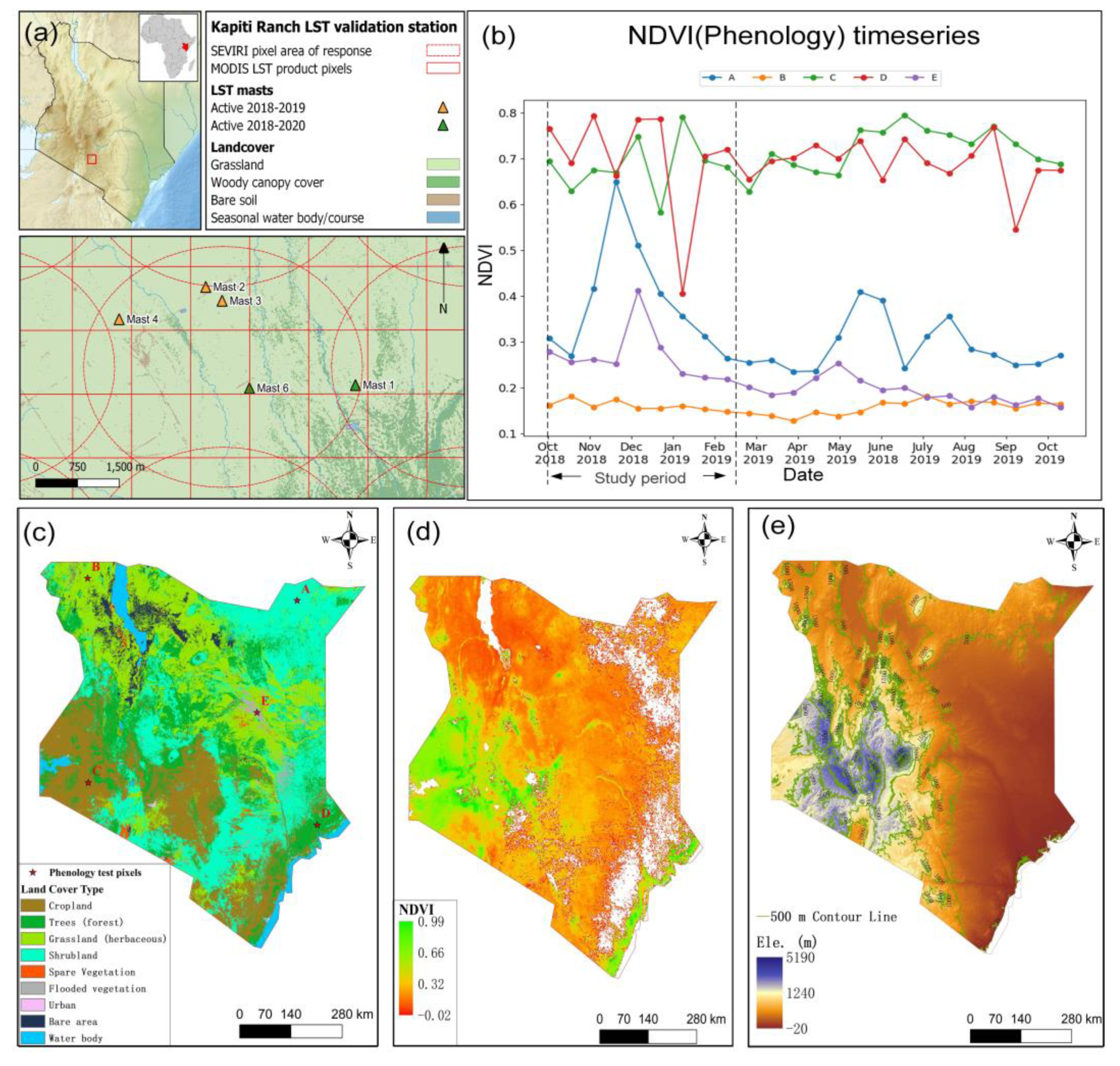
2. Study Area and Datasets

2.1. Study Area and In Situ LST Ground Observations

The study area for this work covers Kenya (East Africa) with a total area of around 582,646 km2. As illustrated in Figure 1, the far southwestern part of the country is characterized by highly vegetated cropland and forest, with complex topography at higher elevations (>1000 m). In contrast, the rest of the region is primarily dominated by flat plains and covered with sparser vegetation types (grass or shrub savannas). Most of Kenya is dominated by Arid (BSh, BWh) and Tropical (Af, Am, Aw) Köppen–Geiger climate zones with some Temperate (Cfb, Csb, Cwb) climate zones found in the south-west [53]. Snow and ice rarely occur except at high altitude. The local climate experiences a bi-modal rainfall pattern, with a season of ‘short rains’ typically between October and December and ‘long rains’ from April to late May or June. Other months are identified as dry seasons. Given the wide range of precipitation, topography and climate types, methodologies for improving LST cloud gap-filling developed in Kenya are likely applicable to many other areas globally, especially in the (sub) Tropics and the Temperate zones.
The ILRI Kapiti Research Station is located in south-west Kenya (−1.6083°, 37.1327°), as shown in Figure 1a. This station is run by the International Livestock Research Institute (ILRI) and provides observations of LST and land surface energy balance, as well as CO2 and H2O fluxes. The observation sites are instrumented using a series of mast mounted (Heitronics) LWIR radiometers to deliver upward (53° view zenith angle) and downward (15° view zenith angle) looking LWIR brightness temperatures. They are then processed to deliver logged LST estimates every 5-min according to the LST in situ measurement principles described in Gottsche et al. [54]. There are four sites in all (Masts 1–4 in Figure 1a) which can provide LWIR radiometer measurements suitable for the evaluation of satellite-based LST products since September 2018. The research station has a fenced 15 km × 20 km area of homogenous savannah, which can further be broken down into 94% grassland-soil complexes and 6% tree canopy cover.
We employ the in situ LST data on Masts 1–4 of ILRI Kapiti Research Station as our primary benchmark (validation) dataset, focusing on the period from October 2018 to February 2019. A brief description of the derivation and accuracy evaluation of our benchmark LST data is provided in the Supplementary Material (Figure S1). The certainty (range of possible error) of the ground observations ranges between 0.79 and 0.95 K per observation throughout the whole time series, across the four masts. The range of possible error consists of radiometric measurement uncertainty, surface emissivity uncertainty, and the uncertainty contribution of the logging equipment as driven by environmental temperature. This time period, encompassing both the short-rains and subsequent dry period, is sufficient in capturing the major climatic and vegetative cycles of an entire year (Figure 1b), by which land surface emissivity and the thermodynamic temperature are strongly affected [55]. In particular, the selected period includes the very rapid green-up (typically only a few days) when the rains start, the rainy sub-period accompanied by increasing vegetation canopy cover, and the sub-period of landscape drying when the rain ends. This phenological pattern is representative of the study area as a whole, as can be seen from the NDVI time series of five typical LWIR pixels in different locations and different land covers across Kenya in Figure 1b. Notice that the locations of the five pixels, i.e., Pixels A (at 3.63° N, 40.35° E), B (4.16° N, 35.23° E), C (0.78° S, 35.22° E), D (0.76° S, 40.84° E), and E (0.93° N, 39.37° E), have been marked in Figure 1c. They are respectively covered by different land use types of shrubland, grassland, cropland, forest, and urban area.

2.2. Satellite Datasets
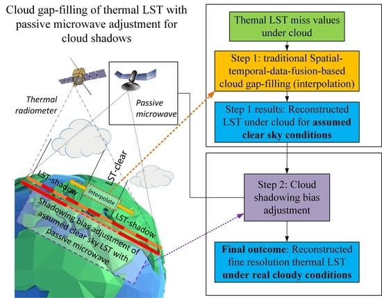
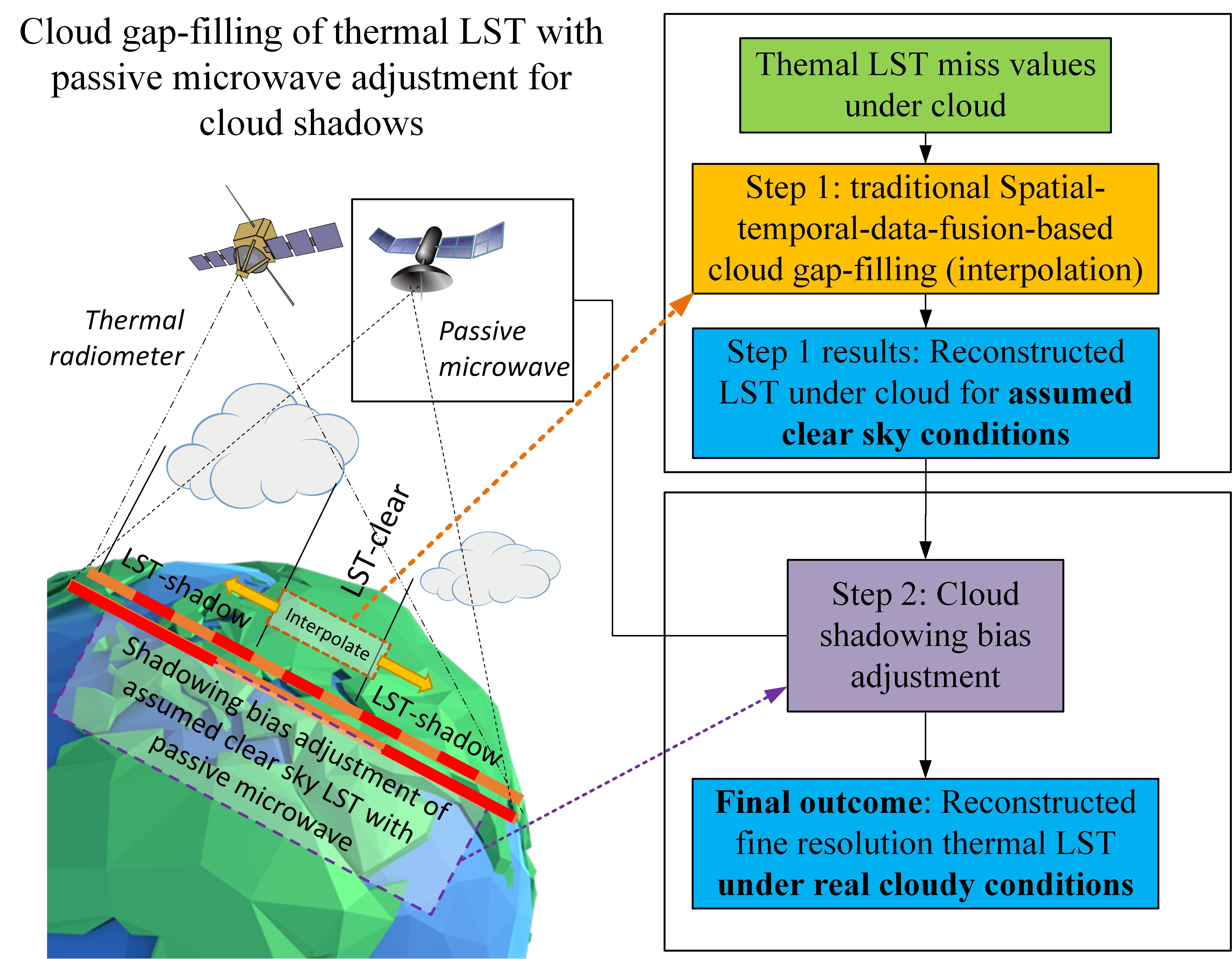
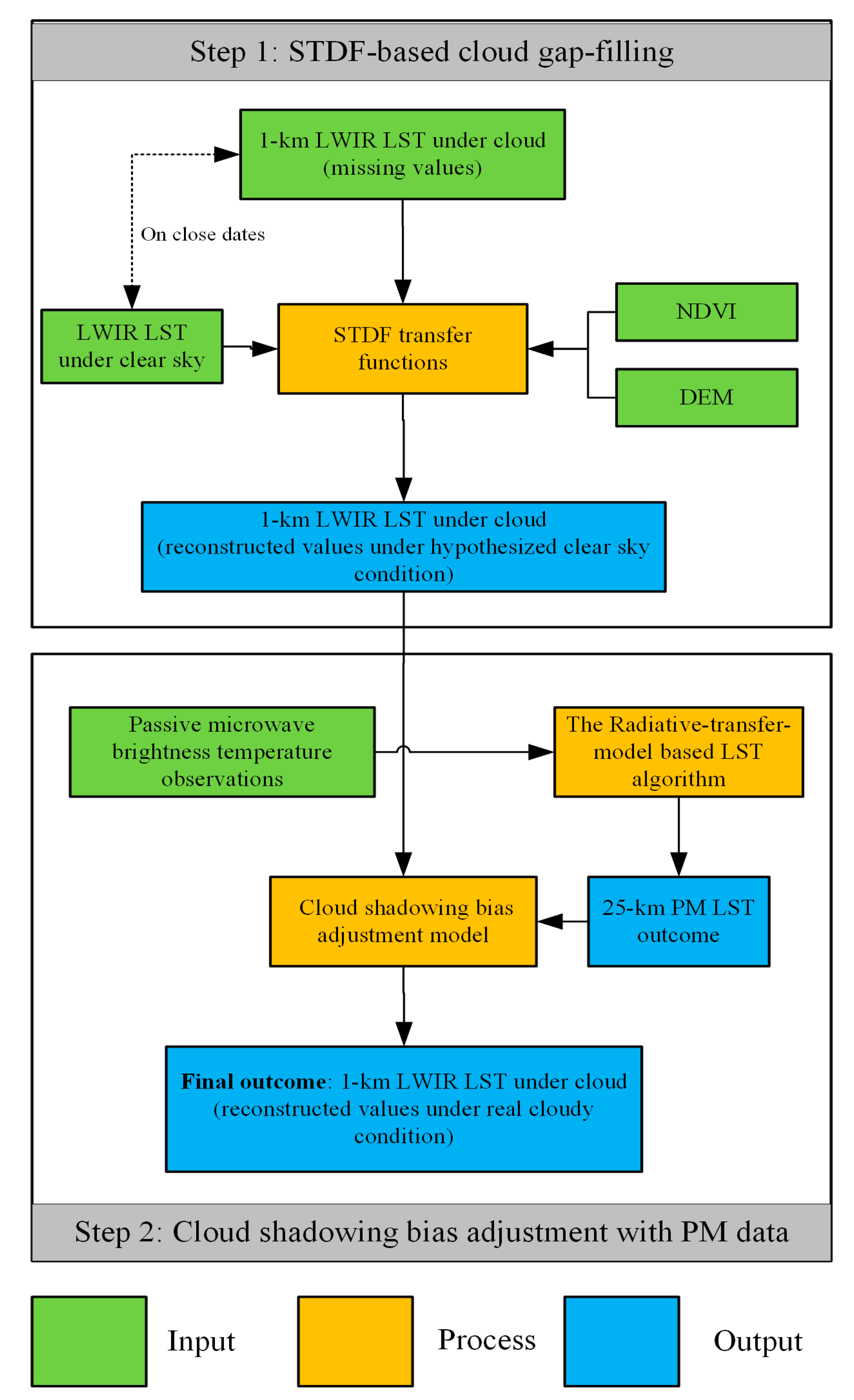
Several satellite datasets were utilized for our study. The enhanced Aqua MODIS 1-km daily LST product (MYD21A1D/N.v061) was selected as the cloud gap-filling target. In addition, we also employed the MODIS MCD43A4 (v061) 500-m daily “Bidirectional Reflectance Distribution Function (BRDF)” adjusted reflectance dataset and the 90-m DEM data generated by the NASA Shuttle Radar Topography Mission (SRTM). The PM data employed are the Level-1R BT data collected by the Advanced Microwave Scanning Radiometer-2 (AMSR-2) operated onboard the Global Change Observation Mission1-Water (GCOM-W1) satellite. The polar orbiting GCOM-W1 was launched by the Japan Aerospace Exploration Agency (JAXA) in May 2012 and shares the same orbital track as Aqua, with a very closing equator-crossing time (about 1:30 p.m./a.m.). The similarity of AMSR-2 and Aqua MODIS observation times is beneficial for blending their observations to fill the gaps of MODIS LWIR LST under cloud.
In addition to the ~5-month in situ data record coming from the ILRI Kapiti Research Station, we also employed the LST data from the geostationary Meteosat platform’s Spinning Enhanced Visible and Infra-Red Imager (SEVIRI) [56] as a second benchmark validation dataset. SEVIRI-derived LST data covering an entire climatic year (from October 2018 to September 2019) were used across the whole Kenya. The SEVIRI LST product is provided every 15 min by EUMETSAT’s Land Surface Analysis Satellite Application Facility (LSA-SAF). Trigo et al. [56] describe the adapted split window algorithm for producing LST data from SEVIRI-measured LWIR brightness temperatures (BTs). Gottsche et al. [54] report that the product has an overall RMSE of 3.2 K compared to LWIR-radiometer derived LSTs collected at a West African validation station located in a tiger bush savanna biome. With a pixel size of around 4 km in Kenya, the primary role of Meteosat LST data was to aid evaluation of both the standard MODIS LST data and the cloud gap-filled MODIS LST data. The latter is possible because instances exist where MODIS pixels classed as cloudy (and thus with no MODIS LST data) are matched by Meteosat LST data that do have an LST observation classed as cloud free within a time lag of up to around 8 min, due to either cloud movements, differences in the cloud masking procedures, and/or due to the different viewing geometries of the two sensors (SEVIRI = ~40–42° view zenith angle (VZA) over Kenya, MODIS VZA = 0–65° depending on overpass). This can be observed in the contrast show in Figure 4c,e in Section 4.

3. Methodology

The flowchart of our cloud gap-filling approach for MODIS LST data is schematically shown in Figure 2. It generally comprises two steps, namely (1) a conventional realization of the STDF methodology and (2) a PM-driven bias adjustment process to calibrate the data coming out of step (1), accounting for the fact that these data should represent cloud-covered rather than clear-sky LSTs. Therefore, there are three datasets tested in the validation step: (i) the clear sky original MODIS product (MODISClear), (ii) MODIS with gaps filled by step (1) (MODISSTDF), and (iii) MODISSTDF bias corrected for under-cloud pixels with passive microwave (AMSR-2) observations (MODISPMBC).

3.1. Step 1: STDF Methodology

3.1.1. Methodology Description

The 1 km MODIS LST data were subset to Kenya and pixels classed as cloud contaminated were removed using the “quality control (QC)” field contained within the MODIS LST product. In addition, all pixels flagged as ‘cloud-edge’ or low quality were also removed. A 500-m daily NDVI dataset for Kenya was calculated using the red-band and infrared-band reflectance data from the MODIS MCD43A4 product, which has been corrected for angular reflectance effects based on the BRDF. The resulting estimates were resampled using a spatial averaging procedure to the same 1-km resolution as the MODIS LST product. The spatial resampling process was also applied to the SRTM DEM dataset subset over Kenya. For each date (represented as t1) in the study period (from October 2018 to September 2019), we used the STDF methodology version detailed in Song et al. [30] to fill cloudy pixels that have no LST data record within the MODIS daily LST product. The Song et al. [30] method was chosen as it has been applied to a large area in South China and obtained relatively good validation performance (with RMSEs between 1.5 and 3.5 K). A summary of the STDF method is given here, whilst the full details can be found in the work of Song et al. [30].
The STDF method first builds a transfer function based on the above-described datasets (LST, NDVI and DEM) as follows:
L S T t 1 = a × L S T t 0 + b × N D V I t 1 + c × D E M + d
where the superscript “*” indicates that this variable has been normalized to the range 0 to 1.0, based on the maximum and minimum values of that variable found across Kenya during our study period. Parameters a, b, c, and d are coefficients fitted using all pixels that have a clear-sky LST estimate on a specific date t1 (LST*t1) and at least one closely preceding date, t0 (LST*t0) (see below for further detail on how this was calculated). NDVI*t1 indicates the corresponding (normalized) NDVI on the t1 date. The NDVI data are available for almost every pixel continuously because the MCD43A4 daily product is generated using 16-day composited reflectance data, and therefore has good resistance to data loss from cloud contamination. Notice that day-time and night-time LST data must be separately treated in this transfer function.
After deriving the coefficients of a, b, c, and d, the Equation (1) transfer function was used to fill all cloudy MODIS LST pixels on the t1 date. For any t1 date included in the study period, the t0 date was iterated among all neighbouring dates of t1 meeting the condition |t0t1| <= 15 days (from the nearest date to the furthest date). An average of the estimated LST values for t0 was then taken where a cloud gap pixel was filled more than once (based on the iterative t0 dates), and the iteration was stopped when the fraction of pixels with effective LST values on t1 was equal to or exceeded 0.9. In the original STDF method of Song et al. [30], the remaining small fraction (<0.1) of cloud gaps was then filled with LST data generated by a conventional inverse distance weighted (IDW) interpolation method [57]. However, the IDW step is not done here in order to avoid bringing in extra interpolation uncertainty that may negatively influence the validation step. The final modification to the original Song et al. [30] method is the use of iteration over all possible dates within a 30-day window (rather than only selecting one t0 date that has a high fraction of clear-sky pixels) to increase the amount of data available to the procedure and therefore improve the applicability to the entire area of Kenya.

3.1.2. Method Sensitivity Analysis

In this section, we conducted sensitivity analysis for the STDF method expressed through Equation (1), in order to explore the existing uncertainty sources of the method which may influence performance of the subsequent bias adjustment process. Considering the linearity of Equation (1) and the fact that there are no interactive components between different input variables, the sensitivity of the output variable LSTt1 to each input variable X (denoting LSTt0, NDVIt1, or DEM) can be expressed as the 1st order partial derivative to X, i.e., ( d L S T ( t 1 ) d X ). It should be noted that these input variables are not normalized between 0–1. The sensitivity was calculated for all iterations conducted during Section 3.1.1. The statistical summary of this sensitivity analysis of the different iterations are reported in Table 2. From Table 2, it is apparent that the difference between daytime and night-time for sensitivity of output LSTt1 against LSTt0 and DEM is low. An LSTt0 difference of 1 K can cause a difference on average of 0.5–0.6 K for the (output) gap filled LST. In comparison an average decrease of about 0.3 K or 0.4 K was observed when elevation rises by 100 m. For NDVI, sensitivity is more important in the daytime compared with night-time, since an NDVI increase of 0.1 can result a decrease >1 K in the gap-filled outcome, while it has an almost negligible effect on the night-time outcomes.

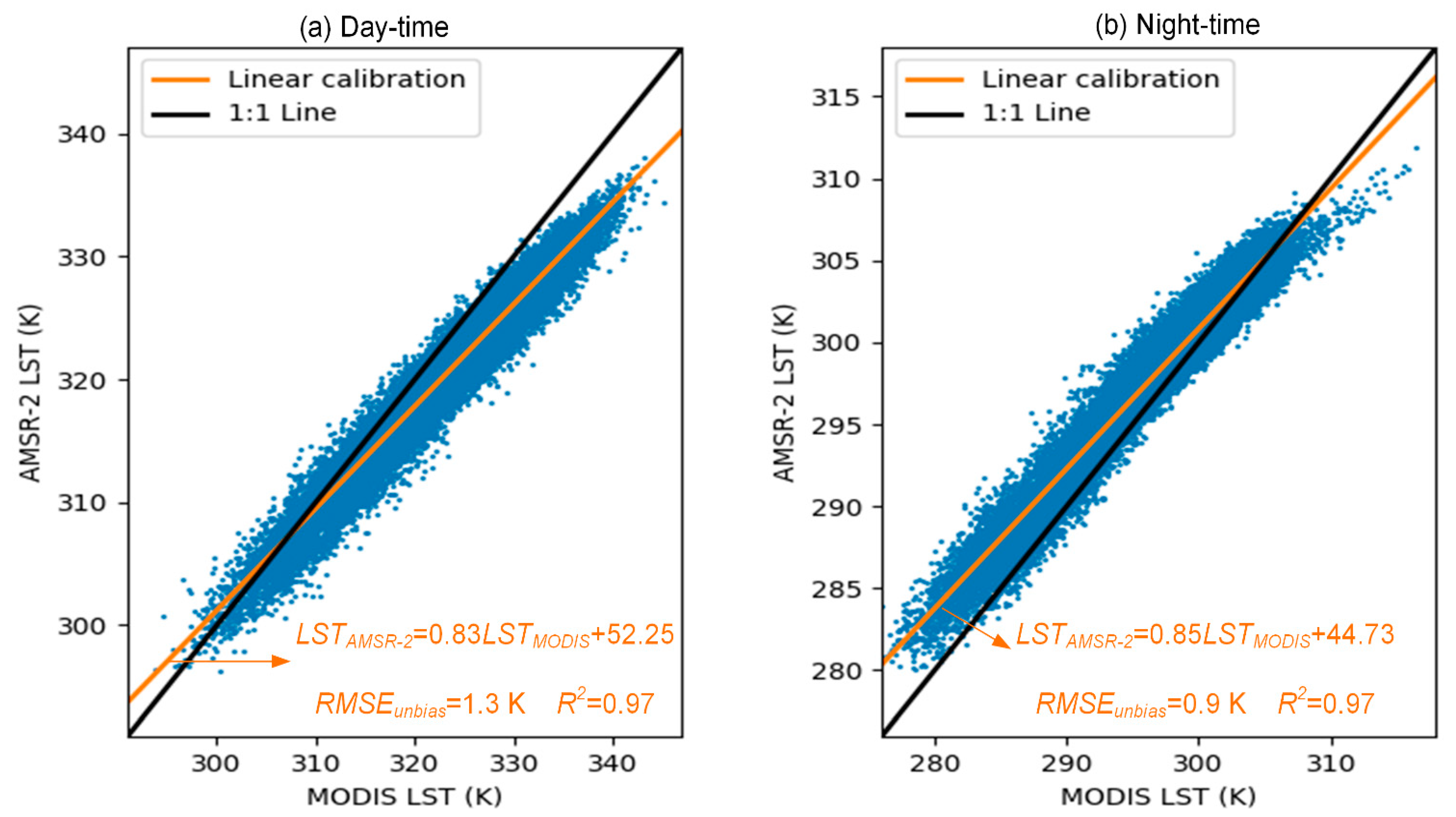
3.2. Step 2: Cloud Shadowing Bias Adjustment with PM-Derived LST Data

As the STDF methodology is based on cloud-free LST observation data from MODIS but is attempting to estimate LST under cloud, biases may be introduced. Identifying and removing such bias is the focus of Step 2 and is based on the AMSR-2 PM-derived LST data. AMSR-2 provides both horizontally (H-) and vertically (V-) polarized BT observations in seven different frequencies [58]. LST data have been estimated by different combinations of these data [59,60,61,62,63], including at 6.9 GHz, 10.7 GHz, 18.7 GHz, 23.8 GHz, 36.5 GHz, and 89 GHz. The linear LST retrieval algorithm based on the 36.5 GHz V-polarized BT [61,64] is among the most widely used, though Song et al. [65] found it inferior to that based on the 18.7 GHz and 23.8 GHz bands [63,66], especially for pixels with higher fractions of water surface (including standing water and dynamic water signals like high levels of soil moisture). To minimize the influence from increased soil moisture on LST retrieval in the rainy season of our study area, we employ the AMSR-2 V- and H-polarized 18.7 GHz and 23.8 GHz BTs to retrieve LST using the methodology of Jones et al. [63]. The resulting PM-derived LST estimates have a spatial resolution of 25 km after the AMSR-2 Level1R BT data were resampled according to the global Equal Area Scalable Earth (EASE) Grid [67] projection system.
The PM BTs at 18.7 GHz and 23.8 GHz have a theoretical temperature sensing depth of around 1 cm [68], as compared to the MODIS LWIR-derived LST skin surface depth of ≤1 mm [69]. To deal with this we first averaged the MODIS 1-km LST data of Kenya to the 25-km EASE Grid and compared those cells that have more than 600 samples (i.e., >95%) of clear-sky MODIS pixels to the AMSR-2 retrieved LST for the same region. As seen in Figure 3, both daytime (ascending) and night-time (descending) MODIS and AMSR-2 LSTs show strong correlations but depart from the 1:1 line. This result agrees with the observations of Song et al. [65], who demonstrated that, apart from in desert and snow/ice covered areas, the LST derived from these two different sensors have a strong linear correlation at the global scale. The AMSR-2 observations have a negative bias of around −0.7 K in the daytime and a positive bias of around 2.5 K in the night-time. This is consistent with the logic that compared to temperature of sub-surface soils, that of skin surface is usually higher at mid-noon but lower at midnight. Therefore, the bias in Figure 3 can be largely ascribed to the different sensing depths. To enable the AMSR-2 LST data to provide the best estimate of what MODIS would have measured, we fit an independent linear equation to the data of day-time and night-time modes respectively, as shown by the orange text in Figure 3. These achieved high coefficients of determination (R2 ≥ 0.9), with RMSEs between the AMSR-2 LST data adjusted via these equations and the true MODIS LST (RMSEunbias) of less than 1.5 K. The small value of RMSEunbias proves a high degree of consistency between PM (AMSR-2)-derived LST and MODIS LWIR LST, thereby confirming the feasibility of the penetration depth bias adjustment process.
Next, we inverted the linear relations in Figure 3 and thus transformed the AMSR-2 based LST data (LSTAMSR-2) into the corresponding best estimate of MODIS-derived LST at the 25-km pixel scale (LSTMODIS_25km):
L S T   M O D I S _ 25 k m = k 0 × L S T A M S R - 2 + m 0
where k 0 and m 0 are the linear relationship parameters found in Figure 3. This removes the penetration depth bias. Data at 1-km resolution can then be further calibrated to remove the cloud shadowing bias based on the relationship:
i = 1 N 1 L S T c l e a r _ s k y _ i + j = 1 N 2 ( L S T c l o u d _ g a p _ j + Δ L S T ) N 1 + N 2 = L S T 25 _ k m
where the number of clear-sky MODIS LST pixels (LSTclear_sky) within a 25-km pixel is N1, and the number of cloud gap-filled pixels (LSTcloud_gap) is N2. We then assume that all cloud gap-filled MODIS pixels within the 25-km AMSR-2 pixel have the same shadowing bias (ΔLST). Therefore, ΔLST for all cloud gap-filled pixels within a certain 25-km grid can be calculated via rearrangement of Equation (3) to:
Δ L S T = L S T 25 _ k m × ( N 1 + N 2 ) i = 1 N 1 L S T c l e a r _ s k y _ i j = 1 N 2 L S T c l e a r _ g a p _ j N 2 ,   if   j = 1 N 2 Δ L S T N 1 + N 2 > R M S E u n b i a s
Equation (4) is constrained with the premise of j = 1 N 2 Δ L S T N 1 + N 2 R M S E u n b i a s . RMSEunbias denotes the fitting errors illustrated in Figure 3 and can be identified as the threshold value for random (non-systematic) error between LST retrievals made at different spatial resolutions. When j = 1 N 2 Δ L S T N 1 + N 2 lies below this threshold the LST error is mainly driven by this random error. The influence of this random error on ΔLST can be exaggerated if (N1 + N2) >> N2. To mitigate such influences, we use (N1 + N2) to substitute N2 as the new denominator in Equation (5) where j = 1 N 2 Δ L S T N 1 + N 2 R M S E u n b i a s . This means that when random error dominates the overall shadowing bias of the 25-km grid, the bias will be equally allocated to all (N1 + N2) MODIS pixels within the grid regardless of whether they are clear sky or cloudy, as in Equation (5):
Δ L S T = L S T 25 _ k m × ( N 1 + N 2 ) i = 1 N 1 L S T c l e a r _ s k y _ i j = 1 N 2 L S T c l e a r _ g a p _ j N 2 + N 1 ,   if   j = 1 N 2 Δ L S T N 1 + N 2 R M S E u n b i a s
Finally, the STDF cloud gap filled LST values are calibrated by the application of ΔLST, as found by Equation (4) or (5) depending on the amount of cloud cover within an AMSR-2 25-km grid cell, to give MODISPMBC.

4. Results

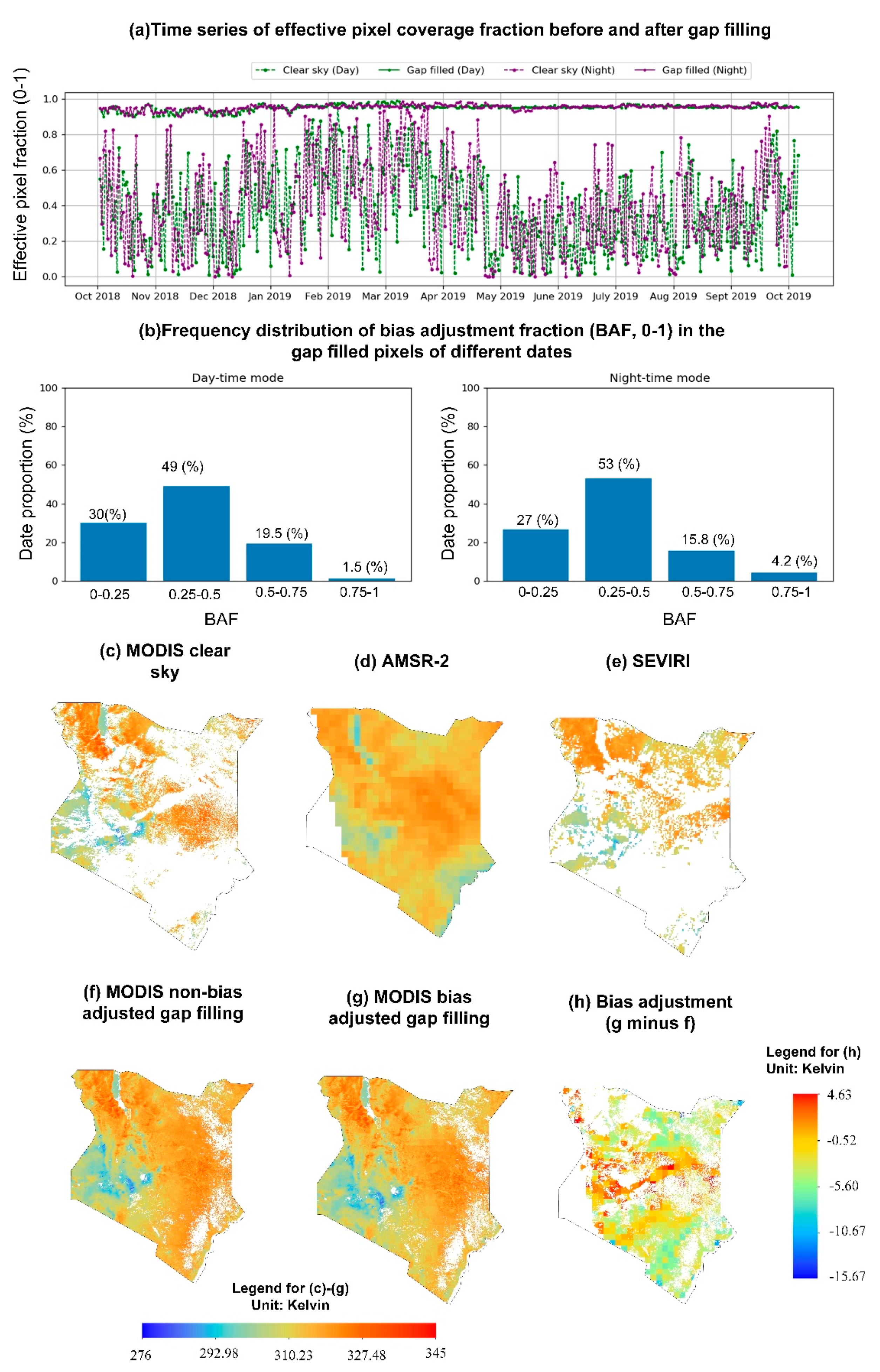
4.1. Overview of Cloud Gap-Filling

Our two-step cloud gap-filling processes improved the spatial coverage of the daily daytime and night-time MODISClear data of Kenya from <50% to >90% for the cloud gap-filled images, as can be seen in Figure 4a. However, it is important to note that the re-visit cycle of AMSR-2 at low latitudes such as those of Kenya is normally greater than a day, so not all cloud gap-filled MODIS LST pixels were able to be bias-adjusted based on a near-simultaneous AMSR-2 observation. Figure 4b shows the proportion distribution of bias adjustment fraction (BAF) for gap-filled pixels of each date. It indicates that BAF on most (≥49%) of dates is between 0.25 and 0.5. Although not high, this rate is sufficient to provide a basis for comparison between the bias adjusted and non-bias adjusted cloud gap-filled LST data. From Figure 4c–h, we employed the day-time data of 22 October 2018 as an example to demonstrate the spatial inputs, outcomes, and corresponding reference data of our methodology. Spatial distribution maps of LST are shown respectively for the non-bias adjusted result in Figure 4f and for the bias adjusted result in Figure 4g. The map of their difference is demonstrated in Figure 4h, revealing that some gap-filled LST values in the middle and south of the country are lower when bias adjustment is included. A series of quantitative validation steps against the reference datasets are carried out in the following sections.

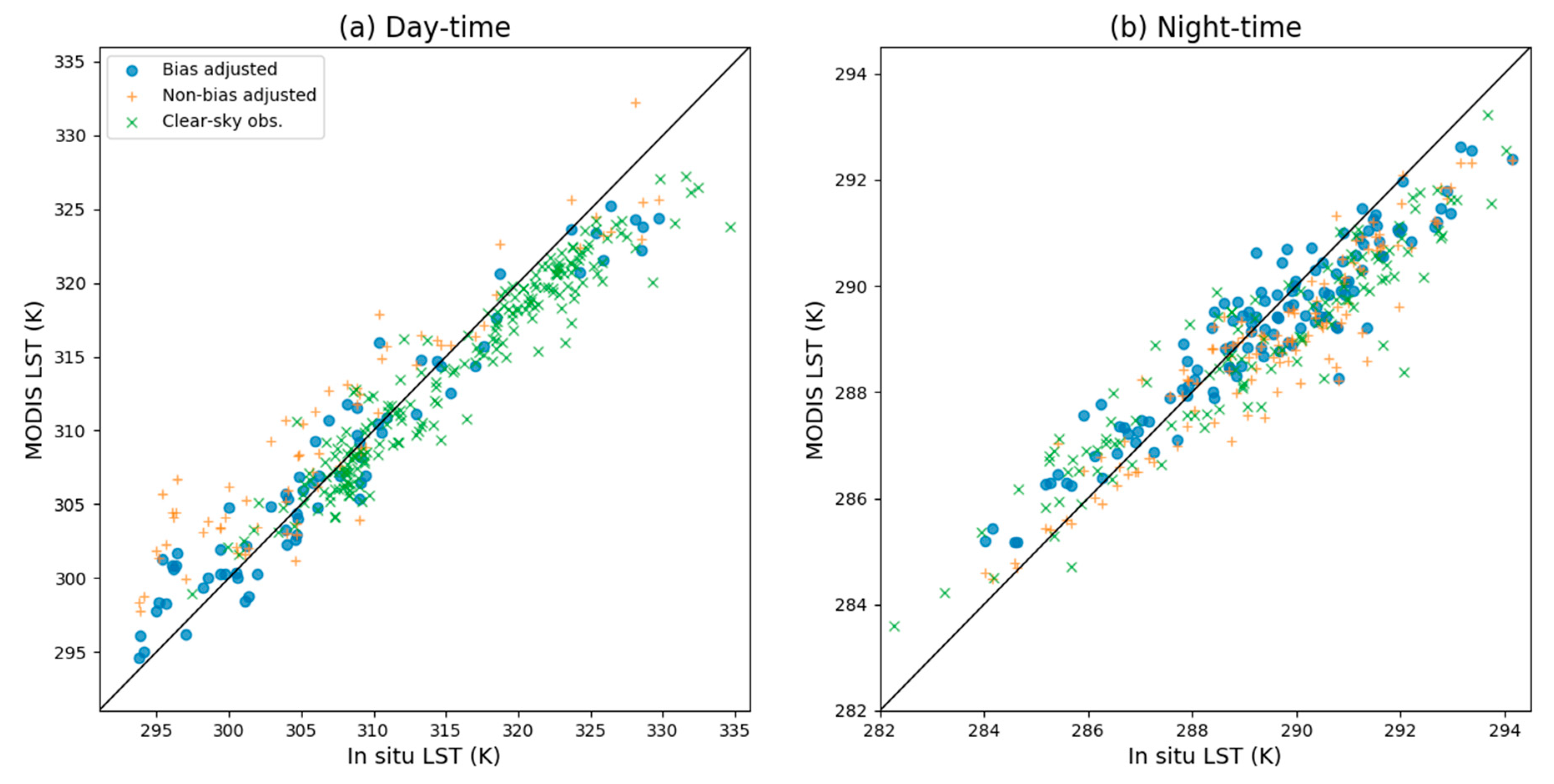
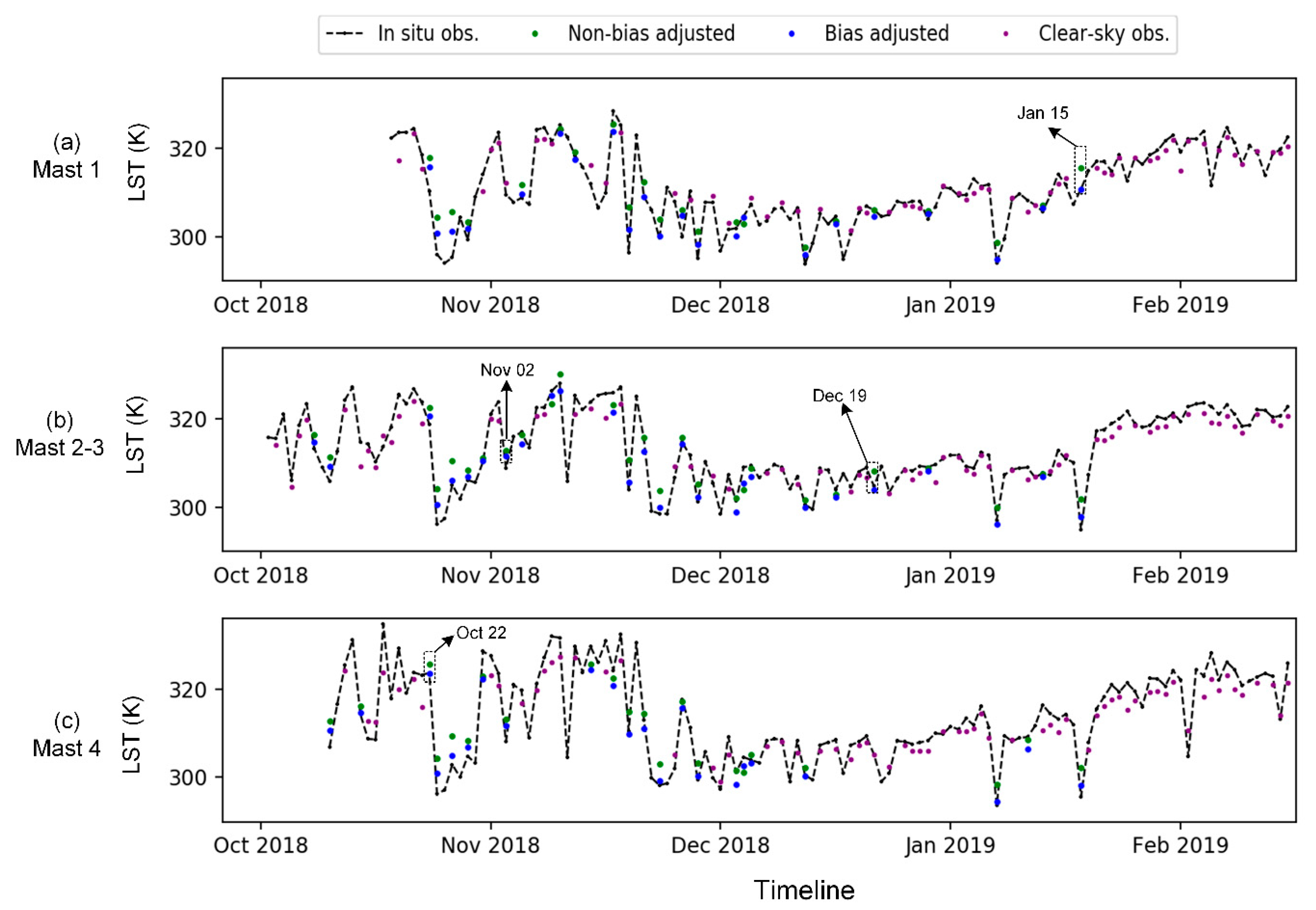
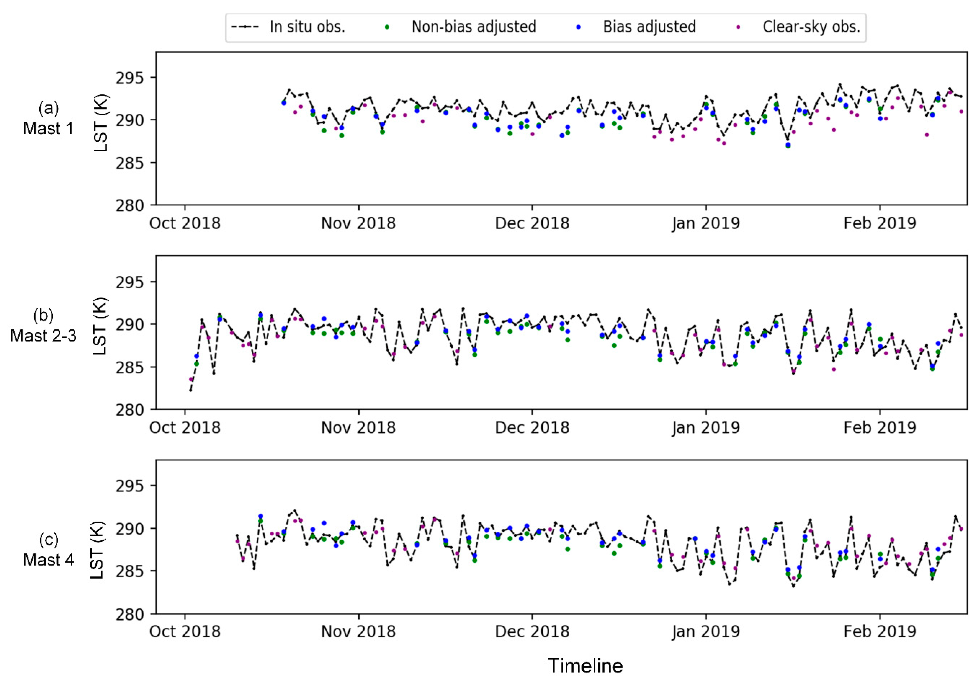
4.2. Validation against In Situ LST Ground Observations

We first compared MODISClear observations from clear-sky pixels, MODISSTDF from Step 1, and MODISPMBC from Step 2, to the contemporaneously collocated in situ LST data recorded at the four masts of the ILRI Kapiti Research Station site (Figure 5 and Table 3). As the local observation times of MODIS and AMSR-2 are reported to have a variation between ±15 min from 13:30 for different dates and different observation swaths, the corresponding in situ data were determined by averaging all in situ LST samples from 13:15 to 13:45 local time (UTC+3) in the day-time, and all in situ LST samples from 01:15 to 01:45 local time at night-time. Moreover, in situ LSTs from Mast 2 and Mast 3 were averaged rather than being used independently, because these masts are in the same 1 km MODIS pixel. The use of multiple masts across and within different pixels (along with the geometric illumination model upscaling method applied, see Section Supplementary Figure S1) means that surface heterogeneity is well accounted for in the landcover under observation. We also examined the gap-filling results against the in situ LST data from Mast 1, Masts 2 and 3 (averaged), and Mast 4 as a time series (Figure 6 and Figure 7). For the time series demonstration, each blue point (MODISPMBC) is accompanied by a corresponding green point (MODISSTDF). Bias adjustments herein are made only on dates where LST estimates are available from both MODIS and AMSR-2. Bias-adjusted outcomes on dates when AMSR-2 data were not available are not shown.
At night, all three datasets show a high degree of agreements with the in situ LST data, with absolute values of mean bias less than 1 K, and RMSEs below 1.5 K. The day-time performance of our cloud gap-filling approach appears poorer than that of night-time, this is likely due to the stronger spatial and temporal variations of LST at noon than at mid-night. However, MODISPMBC agrees significantly better with the in situ LST data record in the daytime than does MODISSTDF. The former has an RMSE of 2.6 K compared to 4.3 K for the non-bias adjusted data, and this is similar to the 2.7 K RMSE shown by MODISClear. Based on all analyses above, the MODISSTDF values tend to overestimate the in-situ data in general, whilst MODISPMBC values are in closer agreement in the daytime. At night, most of the cloud gap-filled satellite estimates are close to the in-situ values, regardless of whether they have been bias-adjusted or not.

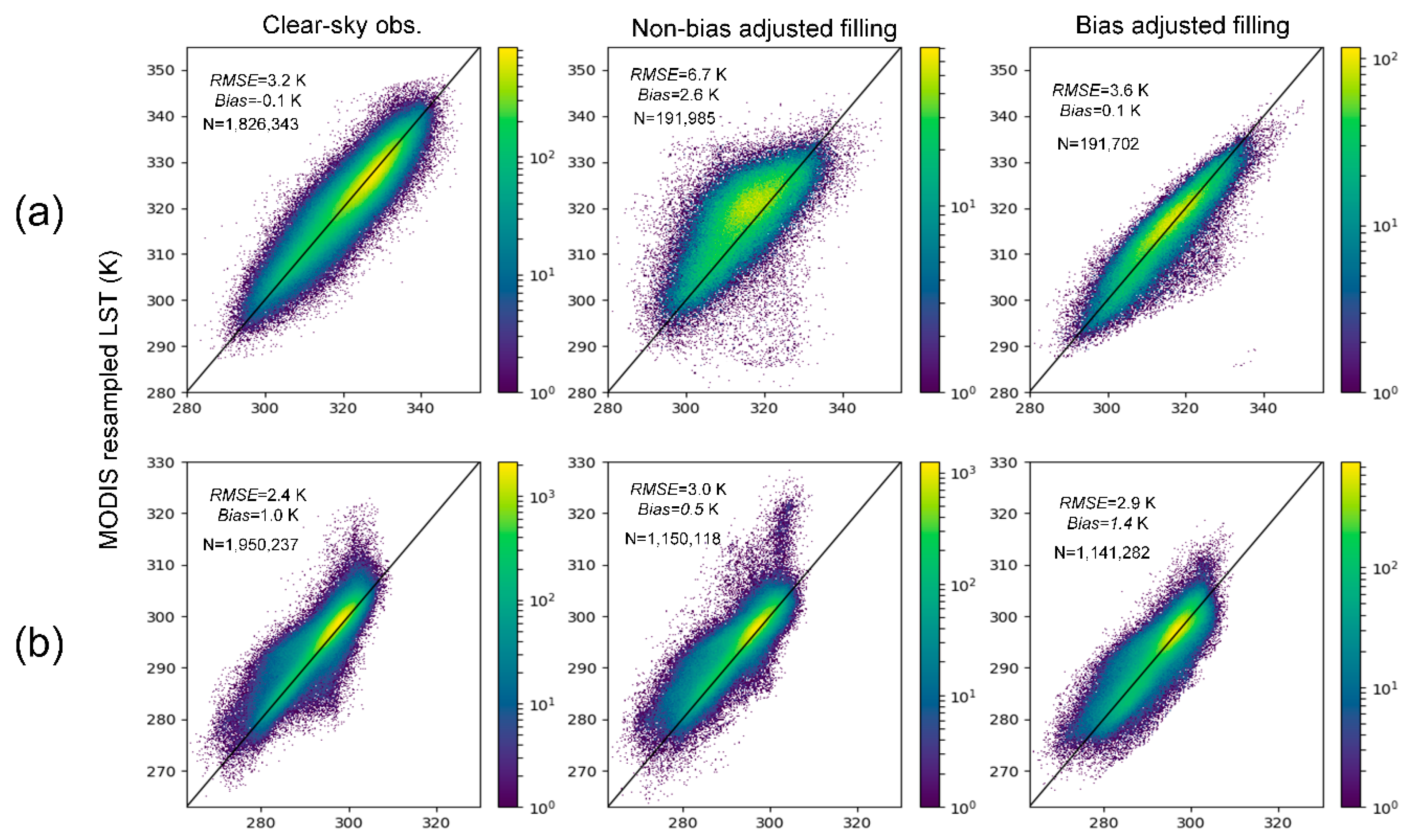
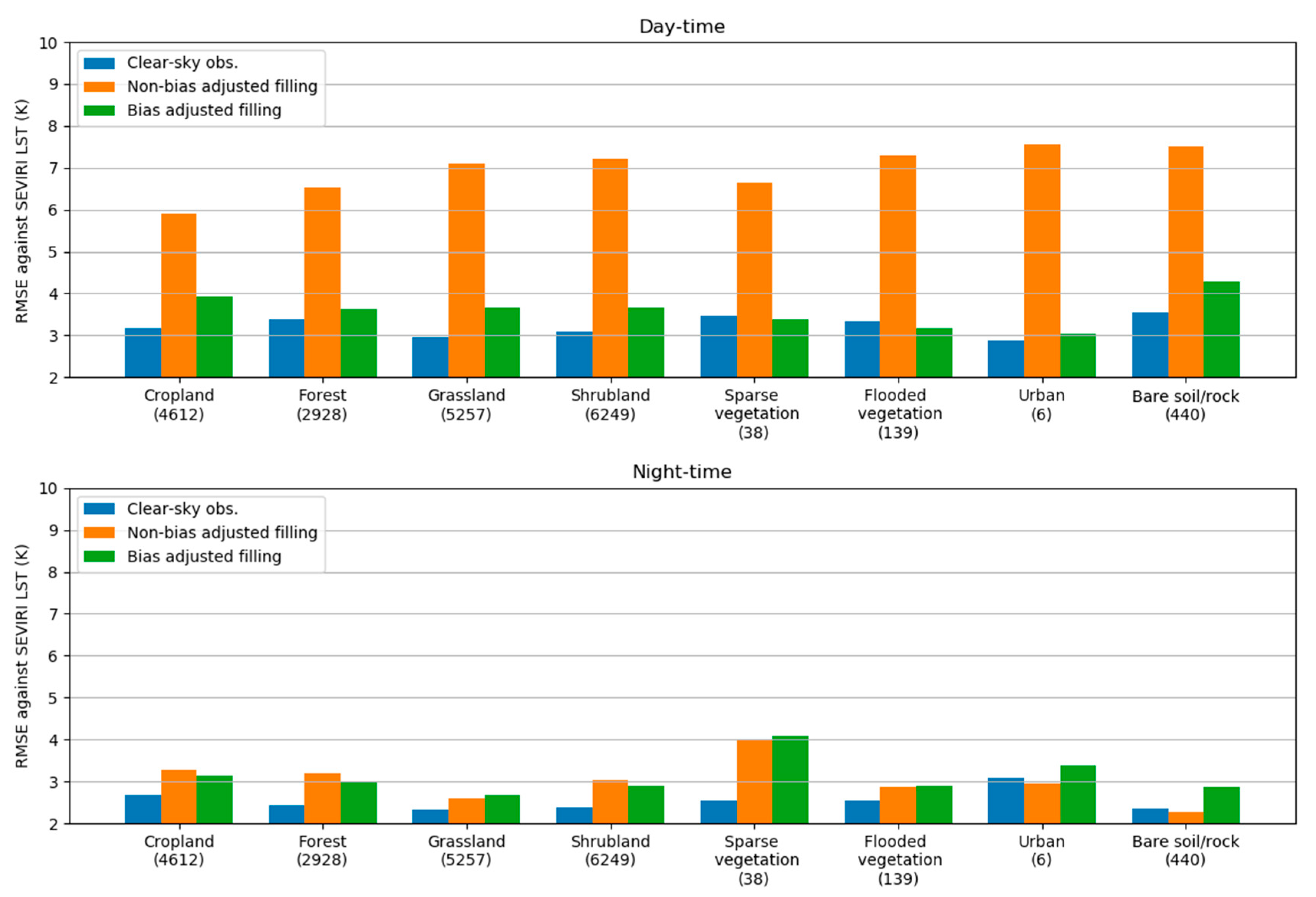
4.3. Validation against SEVIRI Geostationary LST

Our cloud gap-filled MODIS LST data record was also validated against the LSA-SAF Meteosat SEVIRI LST dataset, based on the mean LST of all MODIS pixels within a SEVIRI pixel. This was carried out for the full twelve months of the year. Similar to the evaluation employed against the in situ LST data, SEVIRI data were compared in three independent scenarios. These scenarios are: (1) comparison against only pixels containing clear-sky MODISclear observations; (2) against only pixels that have undergone cloud gap-filling up to Step 1 (MODISSTDF), and (3) against only pixels that have undergone cloud gap-filling up to Step 2 (MODISPMBC) (Figure 8). The temporal means of the SEVIRI-derived LST obtained from the local time of 1:15 p.m./a.m. to 1:45 p.m./a.m. were used for comparison against the spatial means of MODISClear estimates within SEVIRI pixels produced at the corresponding time. To ensure a consistent comparison, only SEVIRI pixels for which ≥14 spatially coincident clear-sky MODIS observations were available (i.e., either all or almost all MODIS pixels within the SEVIRI pixel are identified as cloud free) were considered. The same strategy was also applied to the evaluation schema of MODISSTDF and MODISPMBC. From Figure 8, it is clear that daytime results differ more between clear-sky observations and cloud gap-filled estimates than do the night-time results. In the daytime, the best correspondence between MODIS and SEVIRI LSTs is achieved under clear-sky conditions, with a negligible bias and an RMSE of 3.2 K. The performance of the bias-adjusted cloud gap-filled result is slightly worse, with an RMSE of 3.6 K. However, this is an improvement upon the performance of the non-bias adjusted cloud gap-filled data, where an RMSE of 6.7 K and a positive LST bias of about 2.6 K were observed. At night, the performance of MODISSTDF and MODISPMBC correction is similar, with RMSE no higher than 3.0 K.
Based on the yearly Kenya-wide comparison in Figure 8, further detailed analyses were conducted with respect to independent land cover types and daily timescales, as shown in Figure 9 and Figure 10 respectively. The ESA CCI 300-m land cover map in 2018 (see Figure 1c) was exploited to provide land cover type information for the entirety of Kenya. The areal fraction of each land cover type in Figure 1c (except for water bodies) was calculated for all SEVIRI-viewed pixels (~4 km) within the country. A SEVIRI 4-km pixel containing any given land cover type with area fraction lower than 0.7 is identified as a ‘mixed pixel’ and thus eliminated, while the remaining ‘pure’ pixels were employed to evaluate the potential influence of land cover variation on the gap-filled results, as shown in Figure 9. The similar performance among different land covers was consistent with the overall RMSE results reflected in Figure 8. This suggests that the bias-adjusted cloud gap-filling method is effective over a wide range of vegetation covers in obtaining LST estimates with competitive accuracy against MODIS clear-sky LST observations. The poorest performance of MODISPMBC is found over bare soil/rock during the day (RMSE ≈ 4.2 K) and over sparse vegetation at night (RMSE ≈ 4.0 K). However, this is acceptable considering that the difference between MODISpmbc and MODISclear RMSE is insignificant (<1.5 K).
The daily time series of difference between RMSE for gap-filled LST (MODISSTDF and MODISPMBC) and RMSE for clear sky LST (MODISClear) are demonstrated in Figure 10. The fraction of clear sky LST pixels over the study area for each day are also shown using the red bar on the right-hand y-axis. From the contrast between blue (MODISPMBC) and orange (MODISSTDF) lines, we can see that the relative performance between the bias adjusted gap-filling algorithm against the non-bias adjusted algorithm is stable over different seasons of the year. The performances of the non-bias adjusted vs. bias adjusted algorithms are not significantly influenced by the fraction of clear sky LST pixels that are needed to build the gap-filling model.

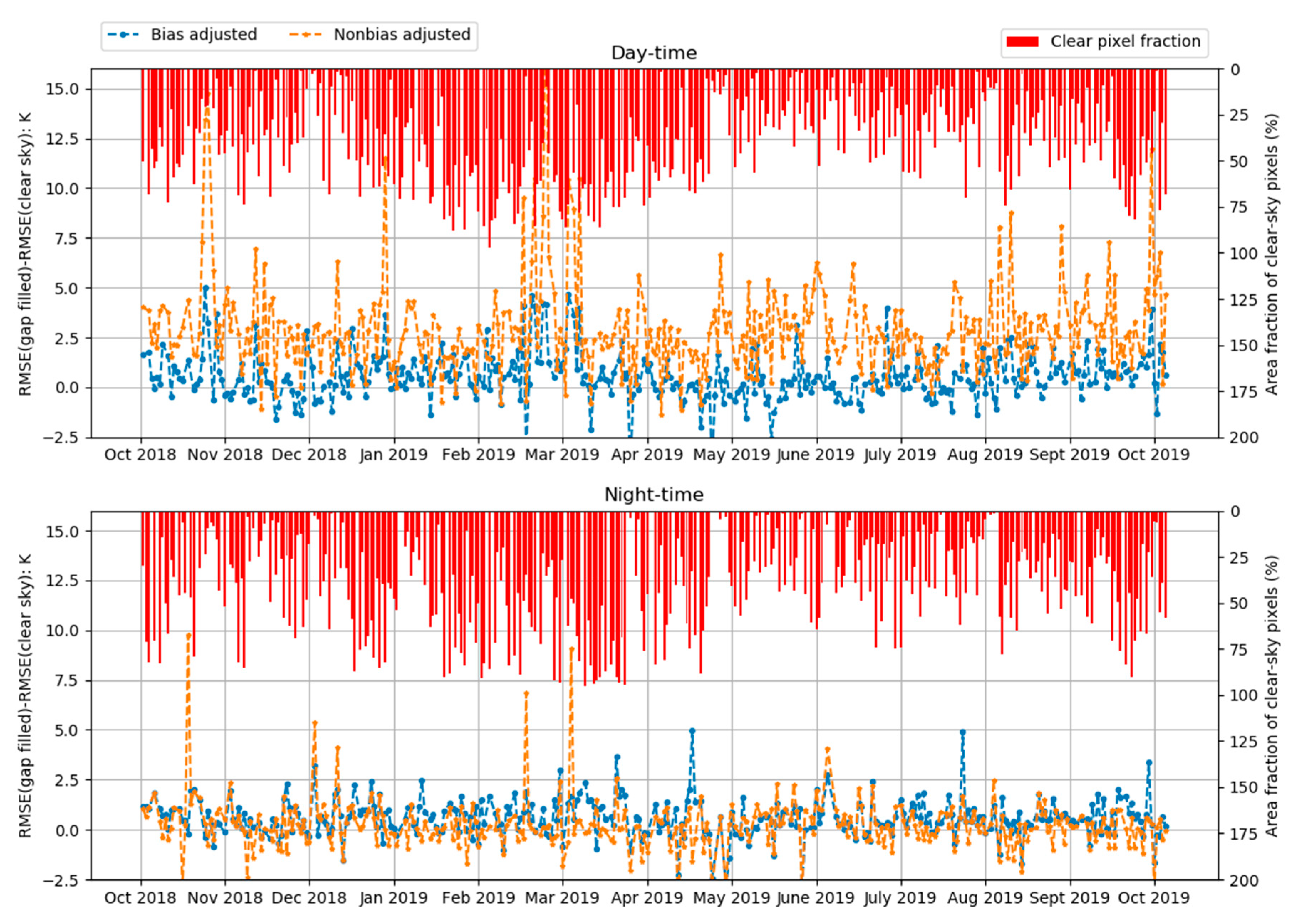
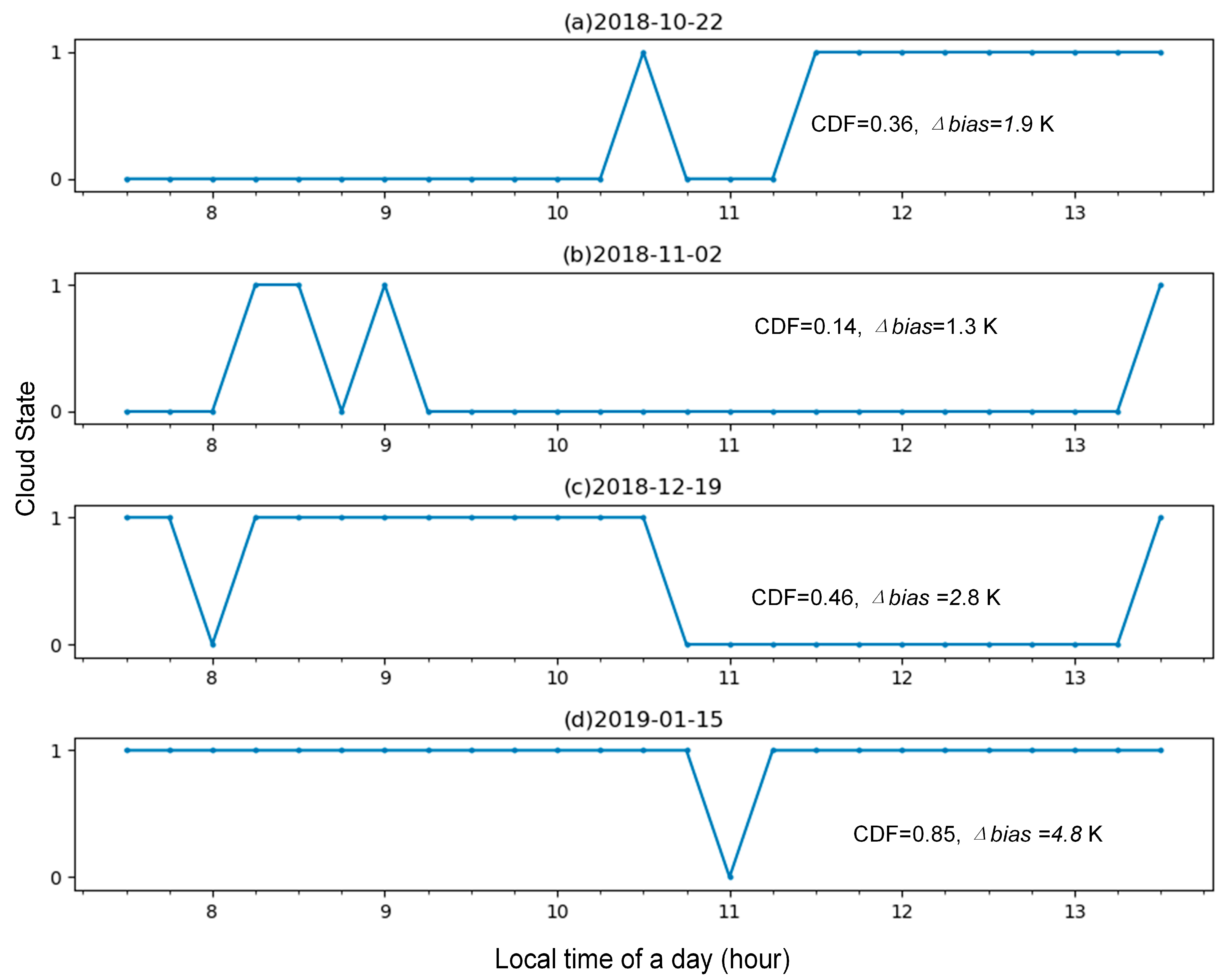
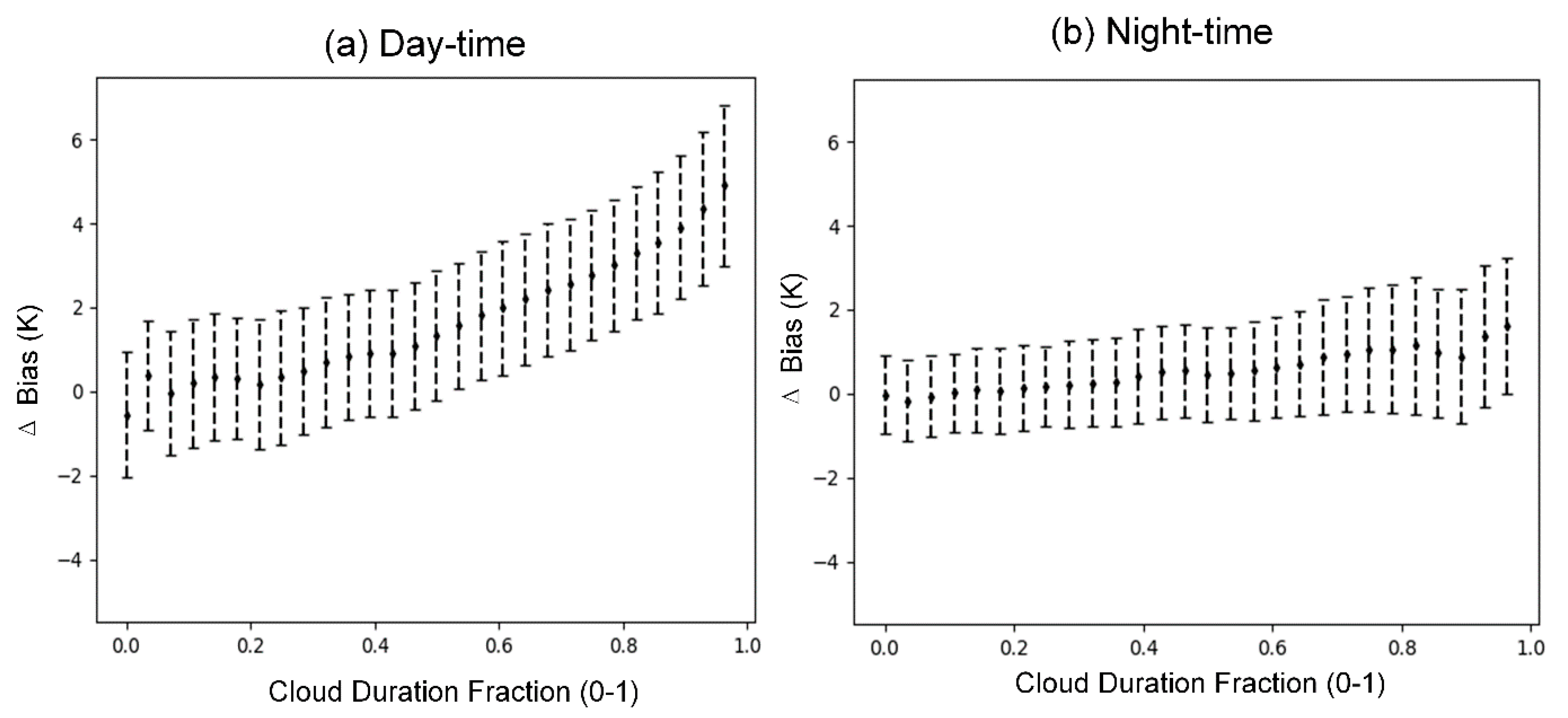
4.4. Influence of Cloud Duration on PM-Based Calibration

As the PM-based bias adjustment was found to have more of an effect in the daytime than at night-time, we further investigated the impact of cloud duration during the day and night on bias correction performance. Firstly, data from the four selected dates highlighted in Figure 6 were employed to calculate an evaluation metric, Δbias. This metric is defined as the difference between the absolute bias of the MODISSTDF (|ΔLSTSTDF|) and that of MODISPMBC (|ΔLSTPMBC|). The Δbias metric (|ΔLSTSTDF| LSTPMBC|) was computed over the pixels in which ground validation masts are located. It can be used as an indicator of the accuracy improvement found through applying the PM-based LST bias-adjustment approach of Step 2. A time series indicating the presence or absence of morning cloud was then generated (1: cloud, 0: clear sky) from 7:30 a.m. to 1:30 p.m. local time for each of the four dates selected. Cloud state was provided by data from the sky-pointing radiometer deployed on the masts at ILRI Kapiti Research Station (see Supplementary Material Section S2, Figure S2). The dates selected for this were chosen at random from the days within four equal divisi)ons of the available time period. Based on this time series, a daily cloud duration fraction (CDF) was calculated, defined as the number of stable (occluded sky for a minimum of 15 min prior to the given minute) cloud minutes from 7:00 a.m. to 1:30 p.m., divided by the total number of minutes in that period. The results are displayed in Figure 11 and suggest that there is a relationship to be explored between Δbias and CDF, especially considering the low Δbias of 1.3 K and a small CDF of 0.14 on 2nd November 2018 as compared to the far higher Δbias (4.8 K) and correspondingly high CDF of 0.85 of the morning of 15 January 2019. Results in Figure 11 suggest that the performance of our bias adjustment methodology in the daytime is influenced by the length of the cloud period experienced during the morning prior to the early afternoon MODIS overpass whose cloudy observations were filled by our proposed method.
To corroborate the relationship found in Figure 11, a further analysis was carried out using the Meteosat SEVIRI LST data, as this data contains cloud masking information that is available over the entirety of Kenya at 15-min intervals. This provides a more extensive test than with the in-situ data alone. A CDF based on the SEVIRI cloud mask was calculated for both daytime and night-time periods, following the same method as detailed above. For the day-time data, the CDF period was slightly extended to between 7:00 a.m. and 2:00 p.m. in order to account for differences in the observation time of the satellite sensors. Similarly, for the night-time data the period between 7:00 p.m. of the previous date and 2:00 a.m.of the observation date was used. Due to the temporal resolution of SEVIRI (15 min) as compared to that of the in-situ data (5 min), only 28 unique CDF values can be obtained in each seven-hour period.
The outcome (Figure 12) is that in the daytime, the mean Δbias rises as the CDF increases from 0 to 1, while the standard deviations are close for all CDF-based groups. This phenomenon, together with the results in Figure 11, indicate that better day-time performance of our bias adjustment strategy is achieved under conditions of higher CDF ranges in the morning, especially when CDF exceeds 0.5. Essentially, longer periods of cloud cover prior to the afternoon Aqua MODIS overpass tend to provide improved performance of the bias adjustment approach. This is logical because, up to a certain limit, the longer a pixel is covered by cloud, the longer it is shadowed from direct sunlight and therefore the larger the temperature difference will be relative to clear-sky conditions. By contrast, at night there is only a very slight increase in Δbias with increasing CDF, probably indicating that the change in LST is more influenced by the presence/absence of solar radiation in the day time rather than by the presence/absence of downwelling atmospheric radiation from cloud layers at night.

5. Discussion

5.1. Improvement and Universality of the Gap-Filling Methodology

Overall, our evaluation of the cloud gap-filled MODIS LST data against the benchmark data, based on both the in situ and Meteosat SEVIRI LST data records, provides a consistent narrative. For day-time Aqua MODIS overpasses gap-filled LST data using the conventional STDF methodology shows a positive bias. This supports our supposition that, if used alone, the STDF approach overestimates LST due to simulating what the LST would be under clear-sky type conditions, whereas in fact the location is or has recently been cloudy. Our results also reveal the effectiveness of using PM observations for calibration of the gap-filled LWIR-derived LSTs, especially during the daytime.
The implementation of this improved two-step cloud gap-filling framework on LST only depends on satellite remote sensing datasets. Compared to the existing methods (Table 1), it is easier to be implemented and is independent from all auxiliary datasets (e.g., reanalysis data) other than satellite remote sensing inputs. Our approach requires much less dependence on the particular environmental characteristics of the study area than some prior works (Table 1), especially when we take into account Figure 10 which shows that the accuracy of this method is not strongly influenced by the varied daily area fraction of cloudy pixels. The performance is stable under periods of continuous cloudy/rainy weather, as can be seen from the time series (e.g., between late November and early December 2018) in Figure 7. Taken together, these tests indicate the greater universality of the proposed method beyond its current study area, as compared to other existing methods.
It is noticeable that we find a relatively inconsequential cloud insulation effect on LST bias correction at night (Figure 12b), as opposed to the effect seen in the morning-to-noon window. The difference between daytime and night-time observations has rarely been discussed in previous studies related to cloud gap-filling of an LWIR-derived LST dataset, with some authors ignoring the problem by only tackling night-time cloud gap-filling [45]. Other works may have failed to find significant day/night differences, because they calibrated against air temperatures rather than the more physically accurate surface temperatures [30,70]. Our findings suggest that the difference between bias-adjusted and non-bias adjusted gap-filled LST, driven by cloud insulation, is less sensitive to ground long-wave outgoing radiation and downwelling atmospheric radiation at night, as compared with the shadowing of solar short-wave incoming radiation during the day.
From Section 2.1 we can see that Kenya is representative of a variety of different geographical settings due to the varied land covers, climate zones and topographical conditions found across the country. Based on the stable evaluation of results across the different land covers in Figure 9, we suggest that the improved two-step cloud gap-filling framework should be effective in the vast majority of vegetation covers ranging from sparsely vegetated soils and grassland to forest found in low- and middle-latitude regions, where most of the world’s human population resides. However, our current method is likely to be unsuitable for use in several land cover types, namely desert and snow/ice covered areas. This is because the temperature difference between microwave observations and LWIR skin surface observations is very high in such landcovers, whilst a conventional linear calibration (as applied in Equation (2)) insufficiently accounts for the depth-induced temperature differences encountered in these areas [65].

5.2. Uncertainty and Limitations of the Current Study

It is important to stress that neither the benchmark datasets (field radiometer derived LSTs and the Meteosat LST product) or the MODISClear data employed in this study represent the ‘absolute truth’ in terms of surface temperature observations, and we do not consider them as such. Each sensor is subject to its own inherent measurement errors. Moreover, measurements observed by the different sensors may differ on account of the heterogenous spatial scales at which observations are made and aggregated over sensor footprint geometry, as well as changes in environmental conditions occurring between non-temporally contemporaneous measurements. As such, we focus here upon the relative difference in performance metrics between the gap filled data (MODISSTDF and MODISPMBC) and MODISClear, rather than the absolute performance of these gap filled products vs. the SEVIRI and field radiometer benchmark LST datasets themselves. For example, using the Meteosat LST product as a benchmark, a relatively large absolute daytime RMSE (3.6 K) was obtained for pixels gap-filled using the MODISPMBC dataset. This value is however much closer to the absolute daytime RMSE value (3.2 K) obtained from the ‘raw’ MODISClear dataset than the RMSE value (6.7 K) obtained using the MODISSTDF dataset, highlighting the effectiveness of our novel cloud gap-filling two-step framework. While the absolute RMSE found between the MODISClear and the benchmark datasets during the daytime was observed to be high (>3 K), exploration of the causes of this discrepancy is beyond the scope of the current study. Furthermore, the validation effort of Gottsche et al. [54] found an average RMSE of 3.2 K for Meteosat SEVIRI data over a similar biome, indicating RMSE values of this magnitude are currently inherent in LWIR LST products in semi-arid savannah regions.
A limitation of the current study is the relatively small number of field-based LST observations available to validate our cloud gap-filling methodology. Radiometer measurements made at the ILRI Kapiti Research Station are temporally limited, spanning a ~5-month period. Fortunately, however, the period is sufficient to capture one entire climatic and vegetation cycle of local land surface (Figure 1b). In the spatial domain, the validation sites only coincide with ground footprints of three distinct 1-km MODIS pixels that are in close geographic proximity to one another relative to the size of the study area. Nevertheless, the establishment and maintenance of even a single site represents a substantial achievement. Indeed, only one other satellite validation site capable of producing similar LST validation data exists anywhere on the African continent and it is not currently operational [54]. In addition, the limited availability of ground validation data has been compensated for to some extent by the intercomparison of the MODIS-derived products against the independent Meteosat SEVIRI LST product [56] at the national scale through an entire climatic year. The intercomparison between the MODIS derived products and the ground/Meteosat-SEVIRI validation data provided consistent results. Prior studies on cloud gap-filling have primarily relied on validation strategies that artificially remove data to create “vacant sub-regions” of the imagery to replicate the presence of cloud gaps but for which the ‘true values’ of the data are actually known [26,71]. However, this strategy is unsuited to evaluating cloud gap-filling of LST data records, since the pixels for which the “true values” of LST are known have actually been observed under clear sky conditions and have thus not experienced the radiation interception effects of clouds that would be the case for ‘true’ cloud-covered LST pixels.
The sensitivity analysis results reported in Table 2 indicate that a theoretical error as large as 100 m in the DEM only leads to a difference of 0.3–0.4 K in LST on average. As the vertical error of the SRTM DEM is reported to be <16 m [72], the uncertainty of elevation data can be effectively neglected. On the other hand, the influence generated by uncertainty in the NDVI data can be much more significant. This is because the generation of daily-scale NDVI data from the 16-day composite MCD43A4 product relies on an assumption that vegetation change is not significant during the 16-day window. Unfortunately, vegetation changes rapidly during the onset of the rainy seasons in Kenya, which may result in a not-insignificant estimation error in NDVI estimates at certain dates. The resultant gap filled LST data is sensitive to such errors, especially during the daytime (as described in Section 3.1.2). Consequently, the differing performance between MODISSTDF and MODISPMBC in the daytime cannot only be attributed to the effects of cloud as performance can also be impacted by NDVI uncertainty, particularly during the onset of the rainy season when rapid vegetation changes occur. However, the impact of cloud effects can still be identified as the primary driver of the performance differences between MODISSTDF and MODISPMBC, based on the positive correlation observed between the CDF and Δbias of the day-time data in Figure 11 and Figure 12. Furthermore, the impact of the bias correction did not get significantly smaller at the rainy periods (typically between April-June and between October-December) in Figure 10.
Finally, despite the potential bias due to clouds as well as the uncertainty of NDVI input not being very significant for the night-time observations in this study, more validation experiments are required in other study areas to test the wider applicability of this finding. Currently, we recommend applying the PM bias correction process to both daytime and night-time data in future studies, in the event that larger night-time errors can arise from factors that were not present in the current study.

5.3. Future Work

Several points remain where further improvements to our approach might be investigated:
(1) Biases calculated at the coarse (25-km) resolution of AMSR-2 are linearly allocated to each cloud gap pixel at the fine (1-km) resolution in the current study, based on an assumption that cloud geometry (e.g., cloud top height, cloud thickness, etc.) is homogenous within the AMSR-2 pixel. However, a bias-adjustment approach that considers the influence of cloud geometry differences at the AMSR-2 sub-pixel scale may offer further performance improvements to the current two-step LST cloud gap-filling framework.
(2) If applying the methodology at continental to global scales, the derived relations between AMSR-2 and MODIS LSTs (Equation (2)) should be re-explored because they are likely dependent on seasonal features and climate types that will vary at the continental/global scales.
(3) As the re-visit cycle of AMSR-2 is greater than one day at low latitudes, better spatial coverage may be achieved by the fusion of AMSR-2 data and data from other PM radiometers.
(4) Cloud gap-filling of Terra MODIS LST data (MOD11A1) could be similarly conducted using data from a PM radiometer similar to AMSR-2, but with local time of overpasses around 10:30 a.m./p.m. One candidate is the microwave radiation imager onboard the Fengyun-3C satellite [73].

6. Conclusions

In this study, we have presented an effective two-step framework for improving the cloud gap-filling performance of the LWIR-based daily land surface temperature (LST) data delivered by Aqua MODIS. The primary innovation of the framework lies in the coupling of a conventional “spatial-temporal data fusion (STDF)” methodology to a cloud shadowing bias-adjustment process, based on passive microwave (PM) LST data derived from the AMSR-2 instrument. We have evaluated the resulting STDF-based cloud gap-filled and PM-bias adjusted LST data against both in situ LST data and the geostationary SEVIRI-derived LST data record. In the daytime, the STDF-based outcomes show an RMSE of 4.3 K against the in-situ data and 6.7 K against the SEVIRI LST data. The RMSEs of the PM bias-adjusted outcomes are 2.6 K and 3.6 K respectively. At night, the performance of bias-adjusted outcome and that of STDF-based outcome are very similar.
Overall, we conclude that, compared to the STDF approach alone, our two-step framework provides a means to improve the performance of cloud gap-filling on LWIR-derived LST through fusion with PM data, although the degree of improvement is far more significant for daytime compared to night-time observations. Finally, we have shown that the day-time accuracy improvements of our two-step approach to cloud gap-filling are increasingly apparent (relative to conventional STDF methods) under the condition of increased cloud cover residence time in the morning-to-noon timeframe. The proposed method has been shown to be stable in terms of RMSE change through time, even under spatially and temporally continuous pixel loss conditions, across a wide range of land cover types. In the future, this method could be applied to the next generation of sub-1 km all-weather LST products at the continental or global scale.

Supplementary Materials

The following are available online at https://0-www-mdpi-com.brum.beds.ac.uk/article/10.3390/rs13173522/s1, Figure S1: Summary of the available in situ LST record (Kelvin) for Kapiti site configuration 1. Data is available when at least one ground observing radiometer is active and returning admissible data. The upscaled mean is only available when at least two radiometer observations are available across all masts. Site time series are the downwelling and emissivity corrected LST values for each mast upscaled to the SEVIRI pixel scale. The final (E) time series is the Kapiti mean LST derived from all four sites and upscaled to the SEVIRI pixel scale. Figure S2: Stable cloud cover analysis for Mast 3. 1 is stable cloud present. 0 is stable cloud not present.

Author Contributions

Conceptualization, P.S., T.P.F.D. and M.C.D.J.; methodology, T.P.F.D. and P.S.; software, P.S. and T.P.F.D.; validation, L.M., T.P.F.D. and P.S.; formal analysis, T.P.F.D. and P.S.; investigation, P.S. and T.P.F.D.; resources, M.J.W.; data curation, P.S.; writing—original draft preparation, T.P.F.D.; writing—review and editing, P.S., T.P.F.D., M.C.D.J., L.M. and M.J.W.; visualization, T.P.F.D. and P.S.; supervision, M.J.W. and J.H.; project administration, M.J.W.; funding acquisition, M.J.W., P.S., T.P.F.D., J.H. and Y.Z. All authors have read and agreed to the published version of the manuscript.

Funding

This work arose from a collaboration funded by the Science and Technology Facilities Council (UK) Newton Fund (STFC) Grant Ref: ST/N006712/1, and National Natural Science Foundation of China (NSFC) Grant Ref: 42001304, 61661136004.

Data Availability Statement

The data presented in this study are available on request from the corresponding author.

Acknowledgments

The authors wish to thank NASA-JPL for providing AMSR-2, MODIS, and DEM datasets free of charge. Thanks is also extended to Simon Hook and Gerardo Rivera of NASA-JPL for the loan of some of the radiometers used at the ILRI Kapiti Research Station as part of the ECOSTESS validation effort. The ILRI Kapiti Research Station site was funded by the UK Space Agency IPP project ‘PRISE’ under the Global Challenge Research Fund (GCRF), and by National Capability funding from NERC provided via the National Centre for Earth Observation (NCEO). Thanks also to our ILRI collaborators: Sonja Leitner, Illona Gluecks and all at ILRI Kapiti Research Station for their tireless efforts in keeping the validation station running.

Conflicts of Interest

The authors declare no conflict of interest.

Abbreviations

TermsAcronym
Land surface temperatureLST
Normalised difference vegetation indexNDVI
the Moderate Resolution Imaging SpectroradiometerMODIS
the Advanced Microwave Scanning RadiometerAMSR
passive microwavePM
spatio-temporal data fusionSTDF
the Global Change Observation Mission1-WaterGCOM-W1
land surface energy balance LSEB
Long wave infraredLWIR
numerical weather prediction NWP
brightness temperatureBT
Global Climate Observing System Essential Climate VariableGCOS-ECV
Visible infrared Imaging RadiometerVIIRS
International Livestock Research InstituteILRI
Shuttle Radar Topography MissionSRTM
digital elevation modelDEM
Japan Aerospace Exploration AgencyJAXA
National Aeronautics and Space AdministrationNASA
European Space AgencyESA
European Organization for the Exploitation of the Meteorologcial SatellitesEUMETSAT
view zenith angleVZA
Land Surface Analysis Satellite Application FacilityLSA-SAF
the Spinning Enhanced Visible and Infra-Red ImagerSEVIRI
quality controlQC
Bidirectional Reflectance Distribution FunctionBRDF
Universal Time CoordinatedUTC
cloud duration fractionCDF
bias adjustment fractionBAF

References

  1. Hollmann, R.; Merchant, C.J.; Saunders, R.; Downy, C.; Buchwitz, M.; Cazenave, A.; Chuvieco, E.; Defourny, P.; de Leeuw, G.; Forsberg, R.; et al. The Esa Climate Change Initiative Satellite Data Records for Essential Climate Variables. Bull. Am. Meteorol. Soc. 2013, 94, 1541–1552. [Google Scholar] [CrossRef] [Green Version]
  2. Khanal, S.; Fulton, J.; Shearer, S. An overview of current and potential applications of thermal remote sensing in precision agriculture. Comput. Electron. Agric. 2017, 139, 22–32. [Google Scholar] [CrossRef]
  3. Quattrochl, D.A.; Luvall, J.C.; Rickman, D.L.; Estes, M.G.; Laymon, C.A.; Howell, B.F. A decision support information system for urban landscape management using thermal infrared data. PERS Photogramm. Eng. Remote Sens. 2000, 66, 1195–1207. [Google Scholar]
  4. Ganci, G.; Vicari, A.; Cappello, A.; Del Negro, C. An emergent strategy for volcano hazard assessment: From thermal satellite monitoring to lava flow modeling. Remote Sens. Environ. 2012, 119, 197–207. [Google Scholar] [CrossRef]
  5. Yao, Y.; Liang, S.; Cheng, J.; Liu, S.; Fisher, J.B.; Zhang, X.; Jia, K.; Zhao, X.; Qin, Q.; Zhao, B.; et al. MODIS-driven estimation of terrestrial latent heat flux in China based on a modified Priestley–Taylor algorithm. Agric. For. Meteorol. 2013, 171–172, 187–202. [Google Scholar] [CrossRef]
  6. Zhang, Y.; Kong, D.; Gan, R.; Chiew, F.H.S.; Mcvicar, T.R.; Zhang, Q.; Yang, Y. Coupled estimation of 500 m and 8-day resolution global evapotranspiration and gross primary production in 2002-2017. Remote Sens. Environ. 2019, 222, 165–182. [Google Scholar] [CrossRef]
  7. Jin, M.S.; Kessomkiat, W.; Pereira, G. Satellite-Observed Urbanization Characters in Shanghai, China: Aerosols, Urban Heat Island Effect, and Land-Atmosphere Interactions. Remote Sens. 2011, 3, 83–99. [Google Scholar] [CrossRef] [Green Version]
  8. Williamson, S.N.; Hik, D.S.; Gamon, J.A.; Kavanaugh, J.L.; Koh, S. Evaluating Cloud Contamination in Clear-Sky MODIS Terra Daytime Land Surface Temperatures Using Ground-Based Meteorology Station Observations. J. Clim. 2013, 26, 1551–1560. [Google Scholar] [CrossRef]
  9. Gutman, G.; Tarpley, D.; Ohring, G. Cloud Screening for Determination of Land Surface Characteristics in a Reduced Resolution Satellite Data Set. Int. J. Remote Sens. 1987, 8, 859–870. [Google Scholar] [CrossRef]
  10. Tomlinson, C.J.; Chapman, L.; Thornes, J.E.; Baker, C. Remote sensing land surface temperature for meteorology and climatology: A review. Meteorol. Appl. 2011, 18, 296–306. [Google Scholar] [CrossRef] [Green Version]
  11. Xu, Y.M.; Shen, Y.; Wu, Z.Y. Spatial and Temporal Variations of Land Surface Temperature Over the Tibetan Plateau Based on Harmonic Analysis. Mt. Res. Dev. 2013, 33, 85–94. [Google Scholar] [CrossRef]
  12. Wan, Z.; Wang, P.; Li, X. Using MODIS Land Surface Temperature and Normalized Difference Vegetation Index products for monitoring drought in the southern Great Plains, USA. Int. J. Remote Sens. 2004, 25, 61–72. [Google Scholar] [CrossRef]
  13. Stathopoulou, M.; Cartalis, C. Use of Satellite Remote Sensing in Support of Urban Heat Island Studies. Adv. Build. Energy Res. 2007, 1, 203–212. [Google Scholar] [CrossRef]
  14. Coppo, P. Simulation of fire detection by infrared imagers from geostationary satellites. Remote Sens. Environ. 2015, 162, 84–98. [Google Scholar] [CrossRef]
  15. Ghaderpour, E.; Vujadinovic, T. The Potential of the Least-Squares Spectral and Cross-Wavelet Analyses for Near-Real-Time Disturbance Detection within Unequally Spaced Satellite Image Time Series. Remote Sens. 2020, 12, 2446. [Google Scholar] [CrossRef]
  16. Su, H.; Liu, J.; Wang, C.; Wang, P.; Huang, J.; Yang, M. Studies on Reconstructing MODIS LST Products Based on Time Series. J. Agric. Sci. Technol. 2014, 16, 99–107. [Google Scholar]
  17. Yan, J.; Shen, R.; Bao, Y.; Li, X. Research on the Reconstructing of MODIS LST Product of Jiangsu Province. Environ. Sci. Technol. 2014, 37, 160–167. [Google Scholar]
  18. Ghafarian Malamiri, H.; Rousta, I.; Olafsson, H.; Zare, H.; Zhang, H. Gap-Filling of MODIS Time Series Land Surface Temperature (LST) Products Using Singular Spectrum Analysis (SSA). Atmosphere 2018, 9, 334. [Google Scholar] [CrossRef] [Green Version]
  19. Frey, C.; Kuenzer, C. Two algorithms to fill cloud gaps in LST time series. In Proceedings of the European Geosciences Union—General Assembly 2013, Vienna, Austria, 7–12 April 2013. [Google Scholar]
  20. Jin, M.L.; Dickinson, R.E. Land surface skin temperature climatology: Benefitting from the strengths of satellite observations. Environ. Res. Lett. 2010, 5, 044004. [Google Scholar] [CrossRef] [Green Version]
  21. Zaksek, K.; Ostir, K. Downscaling land surface temperature for urban heat island diurnal cycle analysis. Remote Sens. Environ. 2012, 117, 114–124. [Google Scholar] [CrossRef]
  22. Linghong, K.E.; Wang, Z.; Song, C.; Zhenquan, L.U. Reconstruction of MODIS LST Time Series and Comparison with Land Surface Temperature (T) among Observation Stations in the Northeast Qinghai-Tibet Plateau. Prog. Geogr. 2011, 30, 819–826. [Google Scholar]
  23. Neteler, M. Estimating daily land surface temperatures in mountainous environments by reconstructed MODIS LST data. Remote Sens. 2010, 2, 333–351. [Google Scholar] [CrossRef] [Green Version]
  24. Stewart, S.B.; Nitschke, C.R. Improving temperature interpolation using MODIS LST and local topography: A comparison of methods in south east Australia. Int. J. Climatol. 2017, 37, 3098–3110. [Google Scholar] [CrossRef]
  25. Yu, W.; Nan, Z.; Wang, Z.; Chen, H.; Wu, T.; Zhao, L. An Effective Interpolation Method for MODIS Land Surface Temperature on the Qinghai-Tibet Plateau. IEEE J. Sel. Top. Appl. Earth Obs. Remote Sens. 2015, 8, 4539–4550. [Google Scholar] [CrossRef]
  26. Sun, L.; Chen, Z.; Gao, F.; Anderson, M.; Song, L.; Wang, L.; Hu, B.; Yang, Y. Reconstructing daily clear-sky land surface temperature for cloudy regions from MODIS data. Comput. Geosci. 2017, 105, 10–20. [Google Scholar] [CrossRef]
  27. Zeng, C.; Shen, H.; Zhong, M.; Zhang, L.; Wu, P. Reconstructing MODIS LST Based on Multitemporal Classification and Robust Regression. IEEE Geosci. Remote Sens. Lett. 2015, 12, 512–516. [Google Scholar] [CrossRef]
  28. Cheng, Q.; Shen, H.; Zhang, L.; Yuan, Q.; Zeng, C. Cloud removal for remotely sensed images by similar pixel replacement guided with a spatio-temporal MRF model. ISPRS J. Photogramm. Remote Sens. 2014, 92, 54–68. [Google Scholar] [CrossRef]
  29. Wang, T.; Shi, J.; Ma, Y.; Husi, L.; Comyn-Platt, E.; Ji, D.; Zhao, T.; Xiong, C. Recovering Land Surface Temperature Under Cloudy Skies Considering the Solar-Cloud-Satellite Geometry: Application to MODIS and Landsat-8 Data. J. Geophys. Res. Atmos. 2019, 124, 3401–3416. [Google Scholar] [CrossRef]
  30. Song, P.; Huang, J.; Mansaray, L.R. An improved surface soil moisture downscaling approach over cloudy areas based on geographically weighted regression. Agric. For. Meteorol. 2019, 275, 146–158. [Google Scholar] [CrossRef]
  31. Zeng, C.; Long, D.; Shen, H.; Wu, P.; Cui, Y.; Hong, Y. A two-step framework for reconstructing remotely sensed land surface temperatures contaminated by cloud. ISPRS J. Photogramm. Remote Sens. 2018, 141, 30–45. [Google Scholar] [CrossRef]
  32. Wang, T.; Shi, J.; Letu, H.; Ma, Y.; Li, X.; Zheng, Y. Detection and Removal of Clouds and Associated Shadows in Satellite Imagery Based on Simulated Radiance Fields. J. Geophys. Res. Atmos. 2019, 124, 7207–7225. [Google Scholar] [CrossRef] [Green Version]
  33. Yang, G.; Sun, W.W.; Shen, H.F.; Meng, X.C.; Li, J.L. An Integrated Method for Reconstructing Daily MODIS Land Surface Temperature Data. IEEE J. Sel. Top. Appl. Earth Obs. Remote Sens. 2019, 12, 1026–1040. [Google Scholar] [CrossRef]
  34. Fu, P.; Xie, Y.H.; Weng, Q.H.; Myint, S.; Meacham-Hensold, K.; Bernacchi, C. A physical model-based method for retrieving urban land surface temperatures under cloudy conditions. Remote Sens. Environ. 2019, 230, 111191. [Google Scholar] [CrossRef]
  35. Zhao, W.; Duan, S.-B. Reconstruction of daytime land surface temperatures under cloud-covered conditions using integrated MODIS/Terra land products and MSG geostationary satellite data. Remote Sens. Environ. 2020, 247, 111931. [Google Scholar] [CrossRef]
  36. Wang, K.C.; Zhou, X.J.; Liu, J.M.; Sparrow, M. Estimating surface solar radiation over complex terrain using moderate-resolution satellite sensor data. Int. J. Remote Sens. 2005, 26, 47–58. [Google Scholar] [CrossRef]
  37. Orth, R.; Dutra, E.; Trigo, I.F.; Balsamo, G. Advancing land surface model development with satellite-based Earth observations. Hydrol. Earth Syst. Sci. 2017, 21, 2483–2495. [Google Scholar] [CrossRef] [Green Version]
  38. Trigo, I.F.; Boussetta, S.; Viterbo, P.; Balsamo, G.; Beljaars, A.; Sandu, I. Comparison of model land skin temperature with remotely sensed estimates and assessment of surface-atmosphere coupling. J. Geophys. Res. Atmos. 2015, 120, 12111–12609. [Google Scholar] [CrossRef] [Green Version]
  39. Johannsen, F.; Ermida, S.; Martins, J.P.A.; Trigo, I.F.; Nogueira, M.; Dutra, E. Cold Bias of ERA5 Summertime Daily Maximum Land Surface Temperature over Iberian Peninsula. Remote Sens. 2019, 11, 2570. [Google Scholar] [CrossRef] [Green Version]
  40. Wang, X.N.; Prigent, C. Comparisons of Diurnal Variations of Land Surface Temperatures from Numerical Weather Prediction Analyses, Infrared Satellite Estimates and In Situ Measurements. Remote Sens. 2020, 12, 583. [Google Scholar] [CrossRef] [Green Version]
  41. Holmes, T.R.H.; Hain, C.R.; Anderson, M.C.; Crow, W.T. Cloud tolerance of remote-sensing technologies to measure land surface temperature. Hydrol. Earth Syst. Sci. 2016, 20, 3263–3275. [Google Scholar] [CrossRef] [Green Version]
  42. Duan, S.B.; Han, X.J.; Huang, C.; Li, Z.L.; Leng, P. Land Surface Temperature Retrieval from Passive Microwave Satellite Observations: State-of-the-Art and Future Directions. Remote Sens. 2020, 12, 2573. [Google Scholar] [CrossRef]
  43. Duan, S.; Li, Z.; Leng, P. A framework for the retrieval of all-weather land surface temperature at a high spatial resolution from polar-orbiting thermal infrared and passive microwave data. Remote Sens. Environ. 2017, 195, 107–117. [Google Scholar] [CrossRef]
  44. Hain, C.R.; Crow, W.T.; Mecikalski, J.R.; Anderson, M.C.; Holmes, T. An intercomparison of available soil moisture estimates from thermal infrared and passive microwave remote sensing and land surface modeling. J. Geophys. Res. Atmos. 2011, 116, D15107. [Google Scholar] [CrossRef]
  45. Kou, X.; Jiang, L.; Bo, Y.; Yan, S.; Chai, L. Estimation of land surface temperature through blending MODIS and AMSR-E data with the bayesian maximum entropy method. Remote Sens. 2016, 8, 105. [Google Scholar] [CrossRef] [Green Version]
  46. Sun, D.L.; Li, Y.; Zhan, X.W.; Houser, P.; Yang, C.W.; Chiu, L.; Yang, R.X. Land Surface Temperature Derivation under All Sky Conditions through Integrating AMSR-E/AMSR-2 and MODIS/GOES Observations. Remote Sens. 2019, 11, 1704. [Google Scholar] [CrossRef] [Green Version]
  47. Zhang, X.; Zhou, J.; Göttsche, F.-M.; Zhan, W.; Liu, S.; Cao, R. A Method Based on Temporal Component Decomposition for Estimating 1-km All-Weather Land Surface Temperature by Merging Satellite Thermal Infrared and Passive Microwave Observations. IEEE Trans. Geosci. Remote Sens. 2019, 57, 4670–4691. [Google Scholar] [CrossRef]
  48. Zhang, X.D.; Zhou, J.; Liang, S.L.; Chai, L.N.; Wang, D.D.; Liu, J. Estimation of 1-km all-weather remotely sensed land surface temperature based on reconstructed spatial-seamless satellite passive microwave brightness temperature and thermal infrared data. ISPRS J. Photogramm. Remote Sens. 2020, 167, 321–344. [Google Scholar] [CrossRef]
  49. Zhang, X.; Zhou, J.; Liang, S.; Wang, D. A practical reanalysis data and thermal infrared remote sensing data merging (RTM) method for reconstruction of a 1-km all-weather land surface temperature. Remote Sens. Environ. 2021, 260, 112437. [Google Scholar] [CrossRef]
  50. Long, D.; Yan, L.; Bai, L.L.; Zhang, C.J.; Li, X.Y.; Lei, H.M.; Yang, H.B.; Tian, F.Q.; Zeng, C.; Meng, X.Y.; et al. Generation of MODIS-like land surface temperatures under all-weather conditions based on a data fusion approach. Remote Sens. Environ. 2020, 246, 111863. [Google Scholar] [CrossRef]
  51. Yoo, C.; Im, J.; Cho, D.; Yokoya, N.; Xia, J.; Bechtel, B. Estimation of All-Weather 1 km MODIS Land Surface Temperature for Humid Summer Days. Remote Sens. 2020, 12, 1398. [Google Scholar] [CrossRef]
  52. Shwetha, H.R.; Kumar, D.N. Prediction of high spatio-temporal resolution land surface temperature under cloudy conditions using microwave vegetation index and ANN. ISPRS J. Photogramm. Remote Sens. 2016, 117, 40–55. [Google Scholar] [CrossRef]
  53. Survey, B.G. Climate of Kenya, Climatic Research Unit at the University of East Anglia, UK, Africa Groundwater Atlas. Climate. British Geological Survey. 2017. Available online: http://earthwise.bgs.ac.uk/index.php/Climate (accessed on 1 June 2021).
  54. Gottsche, F.M.; Olesen, F.S.; Trigo, I.F.; Bork-Unkelbach, A.; Martin, M.A. Long Term Validation of Land Surface Temperature Retrieved from MSG/SEVIRI with Continuous in-Situ Measurements in Africa. Remote Sens. 2016, 8, 410. [Google Scholar] [CrossRef] [Green Version]
  55. Van de griend, A.A.; Owe, M.; Groen, M.; Stoll, M.P. Measurement and Spatial Variation of Thermal Infrared Surface Emissivity in a Savanna Environment. Water Resour. Res. 1991, 27, 371–379. [Google Scholar] [CrossRef]
  56. Trigo, I.F.; Dacamara, C.C.; Viterbo, P.; Roujean, J.-L.; Olesen, F.; Barroso, C.; Camacho-de-Coca, F.; Carrer, D.; Freitas, S.C.; García-Haro, J.; et al. The Satellite Application Facility for Land Surface Analysis. Int. J. Remote Sens. 2011, 32, 2725–2744. [Google Scholar] [CrossRef]
  57. Metz, M.; Rocchini, D.; Neteler, M. Surface Temperatures at the Continental Scale: Tracking Changes with Remote Sensing at Unprecedented Detail. Remote Sens. 2014, 6, 3822–3840. [Google Scholar] [CrossRef] [Green Version]
  58. Du, J.; Kimball, J.S.; Shi, J.; Jones, L.A.; Wu, S.; Sun, R.; Yang, H. Inter-calibration of satellite passive microwave land observations from AMSR-E and AMSR2 using overlapping FY3B-MWRI sensor measurements. Remote Sens. 2014, 6, 8594–8616. [Google Scholar] [CrossRef] [Green Version]
  59. Zhou, J.; Dai, F.; Zhang, X.; Zhao, S.; Li, M. Developing a temporally land cover-based look-up table (TL-LUT) method for estimating land surface temperature based on AMSR-E data over the Chinese landmass. Int. J. Appl. Earth Obs. Geoinf. 2015, 34, 35–50. [Google Scholar] [CrossRef]
  60. Fily, M.; Royer, A.; Goita, K.; Prigent, C. A simple retrieval method for land surface temperature and fraction of water surface determination from satellite microwave brightness temperatures in sub-arctic areas. Remote Sens. Environ. 2003, 85, 328–338. [Google Scholar] [CrossRef]
  61. Holmes, T.R.H.; De Jeu, R.A.M.; Owe, M.; Dolman, A.J. Land surface temperature from Ka band (37 GHz) passive microwave observations. J. Geophys. Res. Atmos. 2009, 114, D04113–D04127. [Google Scholar] [CrossRef] [Green Version]
  62. Prigent, C.; Jimenez, C.; Aires, F. Toward “all weather,” long record, and real-time land surface temperature retrievals from microwave satellite observations. J. Geophys. Res. Atmos. 2016, 121, 5699–5717. [Google Scholar] [CrossRef]
  63. Jones, L.A.; Ferguson, C.R.; Kimball, J.S.; Zhang, K.; Chan, S.T.K.; McDonald, K.C.; Njoku, E.G.; Wood, E.F. Satellite microwave remote sensing of daily land surface air temperature minima and maxima from AMSR-E. IEEE J. Sel. Top. Appl. Earth Obs. Remote Sens. 2010, 3, 111–123. [Google Scholar] [CrossRef]
  64. Owe, M.; Van De Griend, A.A. On the relationship between thermodynamic surface temperature and high-frequency (37 GHz) vertically polarized brightness temperature under semi-arid conditions. Int. J. Remote Sens. 2001, 22, 3521–3532. [Google Scholar] [CrossRef]
  65. Song, P.; Huang, J.; Mansaray, L.R.; Wen, H.; Wu, H.; Liu, Z.; Wang, X. An Improved Soil Moisture Retrieval Algorithm Based on the Land Parameter Retrieval Model for Water-Land Mixed Pixels Using AMSR-E Data. IEEE Trans. Geosci. Remote Sens. 2019, 57, 7643–7657. [Google Scholar] [CrossRef]
  66. Du, J.Y.; Kimball, J.S.; Jones, L.A. Satellite microwave retrieval of total precipitable water vapor and surface air temperature over land from AMSR2. IEEE Trans. Geosci. Remote Sens. 2015, 53, 2520–2531. [Google Scholar] [CrossRef]
  67. Armstrong, R.L.; Brodzik, M.J. An earth-gridded SSM/I data set for cryospheric studies and global change monitoring. Adv. Space Res. 1995, 16, 155–163. [Google Scholar] [CrossRef]
  68. Njoku, E.G.; Li, L. Retrieval of land surface parameters using passive microwave measurements at 6-18 GHz. IEEE Trans. Geosci. Remote Sens. 1999, 37, 79–93. [Google Scholar] [CrossRef] [Green Version]
  69. Korb, A.R.; Salisbury, J.W.; D’Aria, D.M. Thermal-infrared remote sensing and Kirchhoff’s law 2. Field measurements. J. Geophys. Res. Solid Earth 1999, 104, 15339–15350. [Google Scholar] [CrossRef]
  70. Metz, M.; Andreo, V.; Neteler, M. A New Fully Gap-Free Time Series of Land Surface Temperature from MODIS LST Data. Remote Sens. 2017, 9, 1333. [Google Scholar] [CrossRef] [Green Version]
  71. Crosson, W.L.; Al-Hamdan, M.Z.; Hemmings, S.N.J.; Wade, G.M. A daily merged MODIS Aqua-Terra land surface temperature data set for the conterminous United States. Remote Sens. Environ. 2012, 119, 315–324. [Google Scholar] [CrossRef]
  72. Jarvis, A.; Reuter, H.I.; Nelson, H.I.; Guevara, E. Hole-filled SRTM for the Globe Version 4. 2008. Available online: https://cgiarcsi.community/data/srtm-90m-digital-elevation-database-v4-1/ (accessed on 1 June 2021).
  73. Xie, X.; Meng, W.; Dong, K.; Gu, S.; Li, X. In-Orbit Calibration of FengYun-3C Microwave Radiation Imager: Characterization of Backlobe Intrusion for the Hot-Load Reflector. IEEE J. Sel. Top. Appl. Earth Obs. Remote Sens. 2021, 99, 1. [Google Scholar]
Figure 1. Location and geographical settings of the study area, Kenya- Eastern Africa, and the layout of in situ measurement sites located within the study area whose LST data records are used as validation data herein. (a) Upper left, Location of the ILRI Kapiti Research Station in Kenya and the location of the LST validation masts at Kapiti. Inset right- location of Kenya in Africa. Lower pane- Location of the four LST measurement mast sites at ILRI Kapiti Research Station with the approximate response area of the SEVIRI and MODIS pixels over the research station. (b) NDVI time series from MODIS MYD13A2 16-day composite product for five typical pixels (A, B, C, D, and E) across Kenya of an entire phenological year from October 2018 to September 2019. (c) A 300 m resolution land cover classification map of Kenya in 2018 produced by the European Space Agency (ESA) Climate Change Initiative (CCI); (d) An NDVI map of Kenya at 500 m resolution on 22 October 2018, calculated using MODIS MCD43A4 product. Pixels with NDVI < −0.2 (which might indicate water) were screened out. (e) The resampled 1 km resolution map Digital Elevation Model (DEM) of Kenya, derived from the 90m NASA Shuttle Radar Topography Mission (SRTM) dataset (http://srtm.csi.cgiar.org accessed on 7 February 2019).
Remotesensing 13 03522 g001
Figure 2. Flowchart of the proposed cloud gap-filling appraoch proposed for MODIS LWIR LST.
Remotesensing 13 03522 g002
Figure 3. Comparison between land surface temperature (LST) data derived from passive microwave observations made by AMSR-2 and gridded into 25-km pixels, and LSTs derived from near simultaneous Aqua MODIS observations (i.e., the MYD21A1 LST product) averaged over the same 25-km grid cells during the study period. Ordinary least squares linear best fits and the 1:1 lines are shown in solid orange and black respectively.
Remotesensing 13 03522 g003
Figure 4. Demonstration of the cloud gap filling approach for the Aqua MODIS LST data record. (a) Time series of LST fractional coverage of Kenya before and after gap-filling. (b) Proportional distribution of bias adjustment fraction (0–1) in the gap filled pixels of different dates. (ce) Daytime LST maps from the different spaceborne sensors recoded near simultaneously on 22 October 2018, and (f,g) the MODIS LST data of (c) now cloud gap-filled using the methodology detailed herein. All MODIS LST pixels with an NDVI of <−0.2 (indicating the likely presence of surface water) have been screened out in these latter two datasets. (h) A bias adjustment map of cloud gap-filled LST (clear sky pixels eliminated) generated by (g) minus (f).
Remotesensing 13 03522 g004
Figure 5. Comparison of MODISClear (green ‘x’), MODISSTDF (orange plus sign) and MODISPMBC (blue dot) data to corresponding in situ LSTs recorded using the mast-mounted IR radiometers of the ILRI Kapiti Research Station detailed in Figure 1. Day-time data are collected around 1:30 p.m. local solar time, whereas night-time data are around 1:30 a.m. The 1:1 line is also shown, and comparison statistics are presented in Table 3. The clearest benefit of the bias-adjusted gap filling is seen in the coolest temperatures of the day-time record.
Remotesensing 13 03522 g005
Figure 6. Time series of MODIS cloud gap filled daytime LSTs and corresponding in situ LSTs recorded at the locations of (a) Mast 1, (b) Masts 2 and 3 (averaged), and (c) Mast 4 of the ILRI Kapiti Research Station. Note that cloud gap filled LSTs are only shown when both Step 1 and Step 2 of the cloud gap-filling methodology were applied as detailed in Section 3 (“non-bias adjusted” and “bias adjusted” respectively). Dates marked by the box and arrows are those examined in Section 4.4.
Remotesensing 13 03522 g006
Figure 7. Time series of MODIS cloud gap filled night-time LSTs and corresponding in situ LSTs recorded at the locations of (a) Mast 1, (b) Masts 2 and 3 (averaged), and (c) Mast 4 of the ILRI Kapiti Research Station.
Remotesensing 13 03522 g007
Figure 8. Comparison of Aqua MODIS and Meteosat SEVIRI-derived land surface temperatures (LSTs). (a) day-time data and (b) night-time data. MODIS data includes both the clear-sky MODIS LSTs from MYD11A and that output from Step 1 and Step 2 of the cloud gap-filling methodology detailed in Section 3. Colour bars indicate the number of co-located observations within the plotting space.
Remotesensing 13 03522 g008
Figure 9. RMSE of MODISClear, MODISSTDF, and MODISPMBC against SEVIRI LST for different land cover types in the day (top) and in the night (bottom). Numbers in the brackets denote pixel numbers of that specific land cover type.
Remotesensing 13 03522 g009
Figure 10. Difference between RMSE for MODISSTDF (or MODISPMBC) and RMSE for MODISClear, against SEVIRI LST (reflected in the left y-axis), and the fraction of clear sky LST pixels (0–100%) on a daily basis (reflected by the length of red bar in the right y-axis). Results in the daytime and at night-time are shown in the top panel and the bottom panel respectively.
Remotesensing 13 03522 g010
Figure 11. Time series of cloud state reported using the in situ data record from the upward pointing LWIR radiometer installed at the ILRI Kapiti Research Station between 7:30 a.m.–1:30 p.m. for the four dates selected and reported in Figure 6, (a) 22 October 2018; (b) 2 November 2018; (c) 19 December 2018; and (d) 15 January 2019. A value of 1 = stable cloud was present for at least the prior 15 min, whilst a value of 0 = stable cloud was not present for the 25 min prior to the LST derivation. Cloud duration fraction (CDF) and Δbias values are reported for each sub-Figure and defined at the start of Section 4.4.
Remotesensing 13 03522 g011
Figure 12. Outcome of the cloud duration analysis for the whole of Kenya with SEVIRI. Mean (solid point) and standard deviations (dotted line) of the evaluation metric Δbias of cloud gap-filled MODIS LST dataset according to different cloud duration fraction (CDF) groups. The evaluation is made at the pixel level of SEVIRI observations (pixel sizes of around 4 km over Kenya). This analysis highlights that during the day, the STDF+PMBC approach results in improved performance over the STDF-only approach, and this improvement increases with cloud residence time, as indicated by CDF. At night, bias correction offers little additional performance improvement.
Remotesensing 13 03522 g012
Table 1. Summary of LWIR and Passive Microwave data fusion studies related to the production of ‘all-weather’ daily LST information at a higher spatial resolution than PM data alone can produce.
StudyMain Method DescriptionSpatial ScaleLimitations
1. Kou et al. [45]A Bayesian Maximum Entropy (BME) blending approach to merge PM and LWIR data, achieving a Root Mean Square Error (RMSE) in LST of between 2.3–4.5 K.A relatively small 100 × 100 km2 regionOnly used on night-time data over a small region, with its universality requiring more validation.
2. Duan et al. [43]An empirical model based on a digital elevation model (DEM) and clear sky LWIR-derived LST at neighboring pixels to downscale PM-derived data for achieving LST of cloudy LWIR pixels.China Downscaling of PM LST only relies on DEM, may be theoretically less effective in areas where the topographical variation is not important (e.g., low altitude plains).
3. Sun et al. [46]A downscaling method for PM LST using NDVI and DEM data applied for gap-filling of LWIR LST at a finer resolution.China(1) Penetration depth difference between PM and LWIR not considered.
(2) The method was applied over a large area but only validated at limited sites.
(3) PM data were downscaled to 5 km but the feasibility of the method at a finer resolution (e.g., 1 km) requires further investigation.
4. Zhang et al. [47];
Zhang et al. [48];
Zhang et al. [49];
A temporal component decomposition developed for merging observations that achieved a 1-km all-weather daily LST data.Northeastern China;
the Tibetan Plateau
Both microwave data and reanalysis data are required as essential inputs to reconstruct the real LST under cloud. But this increases the complexity of the method and risks increased uncertainty from data inputs. Therefore, it should be cautiously discussed when applied in other regions.
5. Long et al. [50]A data fusion method used to merge LWIR observations and PM-like coarse-resolution reanalysis datasets, based on correlations between images taken a limited time apart.3 plots of 80 × 80 km2 in China(1) This time-interpolation-like fusion method has strict requirement on the availability of its input datasets at neighboring dates [49].
(2) The method only addresses situations of temporally discontinuous pixel loss across relatively small study regions.
6. Yoo et al. [51];
Shwetha and Kumar [52]
Machine-learning based models to fuse LST at different spatial scales.South Korea, about 10,000 km2;
Cauvery river basin in India, about 80,000 km2
The physics behind machine learning models remains unclear, and it is difficult to justify the global universality of these models when the relationships they derive cannot be explicitly formalized.
Table 2. Statistical results for sensitivity analysis of the STDF method during the selected study period. The upper and lower threshold of the indicator are respectively defined as the 90th and 10th percentile of all result samples rather than the maximum and minimum values, in order to avoid outliers.
Sensitivity of LST(t1) on the
Input Variables X, i.e., ( d L S T ( t 1 ) d X )
Observation TimeAverageStandard
Deviation
Upper Threshold
(90th Percentile)
Lower Threshold
(10th Percentile)
NDVI (K/0.1)Day-time−1.110.892.88−4.28
Night-time−0.060.170.76−0.93
DEM (K/100 m)Daytime−0.420.351.21−6.30
Night-time−0.360.421.43−5.69
LST(t0) (K/K)Daytime0.500.841.72−0.80
Night-time0.590.251.49−0.71
Table 3. Statistics resulting from the LST comparison shown in Figure 5. ** indicates significance at p < 0.05.
MODIS LST
Data Type
RMSE (K)Mean Bias (K)rN
DayMODISClear2.7−1.60.96 **198
MODISSTDF4.32.50.94 **71
MODISPMBC2.60.20.97 **71
NightMODISClear1.1−0.40.93 **115
MODISSTDF1.0−0.60.93 **119
MODISPMBC0.8−0.20.94 **119
Publisher’s Note: MDPI stays neutral with regard to jurisdictional claims in published maps and institutional affiliations.

