
A New Method for Crop Row Detection Using Unmanned Aerial Vehicle Images


1
Institute of Geographic Sciences and Natural Resources Research, Chinese Academy of Sciences, Beijing 100101, China
2
Jiangsu Center for Collaborative Innovation in Geographical Information Resource Development and Application, Nanjing 210023, China
3
National Earth System Science Data Center, National Science and Technology Infrastructure of China, Beijing 100101, China
4
University of Chinese Academy of Sciences, Beijing 100049, China
5
Cotton Institute, Xinjiang Academy of Agricultural and Reclamation Science, Shihezi 832000, China
*
Author to whom correspondence should be addressed.
Remote Sens. 2021, 13(17), 3526; https://0-doi-org.brum.beds.ac.uk/10.3390/rs13173526
Submission received: 3 July 2021
/
Revised: 1 September 2021
/
Accepted: 3 September 2021
/
Published: 5 September 2021
(This article belongs to the Special Issue Crop Growth Monitoring Using Remote Sensing: Progress, Challenges and Opportunities)
Abstract
:Crop row detection using unmanned aerial vehicle (UAV) images is very helpful for precision agriculture, enabling one to delineate site-specific management zones and to perform precision weeding. For crop row detection in UAV images, the commonly used Hough transform-based method is not sufficiently accurate. Thus, the purpose of this study is to design a new method for crop row detection in orthomosaic UAV images. For this purpose, nitrogen field experiments involving cotton and nitrogen and water field experiments involving wheat were conducted to create different scenarios for crop rows. During the peak square growth stage of cotton and the jointing growth stage of wheat, multispectral UAV images were acquired. Based on these data, a new crop detection method based on least squares fitting was proposed and compared with a Hough transform-based method that uses the same strategy to preprocess images. The crop row detection accuracy (CRDA) was used to evaluate the performance of the different methods. The results showed that the newly proposed method had CRDA values between 0.99 and 1.00 for different nitrogen levels of cotton and CRDA values between 0.66 and 0.82 for different nitrogen and water levels of wheat. In contrast, the Hough transform method had CRDA values between 0.93 and 0.98 for different nitrogen levels of cotton and CRDA values between 0.31 and 0.53 for different nitrogen and water levels of wheat. Thus, the newly proposed method outperforms the Hough transform method. An effective tool for crop row detection using orthomosaic UAV images is proposed herein.
1. Introduction
To increase economic benefits and reduce environmental impact, precision farming is recommended to farmers [1]. Precision agriculture requires the application of fertilizer, pesticides, irrigation and other field management practices according to the needs of crops [2]. To realize precision agriculture, an accurate prediction of the crop growth status in the field, followed by the generation of site-specific management practice maps, is very important [3,4,5]. Most crops are grown in rows to increase light exposure, enhance gas exchange and facilitate weeding and fertilization. Thus, with respect to the generation of a precision site-specific management practice map, the location of the crop rows in the field must be considered.
Remote sensing is a good tool for crop row detection in the field. Many studies have been conducted using field images obtained by digital cameras or multispectral sensors mounted on autonomous tractors or robots to recognize the location of crop rows and then facilitate real-time tractor or robot navigation [6,7,8]. However, to create site-specific management practice maps for a large field considering the location of crop rows, row detection by field images is not efficient due to its limited observation scope [9]. In addition, satellite or manned airborne imaging for row detection is limited by the spatial resolution, high operational costs, or long delivery of products [10]. Compared with the abovementioned platform, the images acquired by a low-altitude unmanned aerial vehicle (UAV) carrying sensors with a nadir view can be processed into an orthomosaic image of the whole field with a high spatial and temporal resolution. This seems more suitable for the recognition of crop rows and applications in field-scale precision agriculture. Thus, research on crop row detection methods for UAV images is of great significance.
Considering crop row detection using UAV images, the Hough transform-based method is the most commonly used strategy [11]. It involves a series of specific methods that all adopt the Hough transform to identify crop row lines, although they differ in the object on which the Hough transform is performed. The Hough transform was proposed by Hough for machine recognition of complex lines in photographs or other pictorial representations [12]. The principle of the Hough transform involves transforming each of the image points into a straight line in a parameter space, and the peak point in the parameter space corresponds to the line in the original image [13]. The parameter space is defined by the parametric representation used to describe lines in the image plane and collinear points in the image plane which intersect at a point in the parameter space. Based on multispectral images from UAVs, Pérez-Ortiz et al. detected row lines of sunflowers by performing the Hough transform on sunflower/background binary images and then successfully extracted the weeds between rows [14]. Using red, green and blue (RGB) color component images measured by UAVs, Weiss and Fared performed the Hough transform on vine/background binary images to detect vine row orientation, which is an important parameter to describe vineyard 3D macrostructures [15]. Based on RGB images obtained from UAVs, Su et al. successfully detected corn rows by performing the Hough transform on representative points of corn rows that were considered to be located in the crop row line [16]. However, the Hough transform-based method has difficulties in selecting the peak point in the parameter space [17], and it may detect error lines that are not parallel to the crop rows [18]. Thus, it is not sufficiently accurate for crop row detection.
The least squares fitting-based method has been used for row detection in field images to facilitate real-time tractor or robot navigation [19,20,21]. It involves a series of specific methods that all contain data processing steps in which least squares fitting is performed using a series of detected representative row points to obtain the location of each row. However, these methods differ in how they find and classify the representative points to each row. The earliest research was reported by Billingsley and Schoenfisch [19]. They scanned each image row to find the position where the data changed from ‘light’ to ‘dark’ or vice versa. These positions were considered the edges of the rows and were then used to calculate the representative points for the rows. Subsequently, a small window that contained only a single crop row was used to classify the representative points for each row and fit the row line curve using least squares fitting. During this process, the window used a self-adjustment strategy to continuously change its position in the image, and the validity of each regression was assessed by calculating the moment of inertia of the pixels of the window with regard to the candidate row. After Billingsley and Schoenfisch, Søgaard and Olsen also [20] used a least squares fitting-based method to recognize rows of small-grain crops. In their method, the image is divided into a series of small horizontal strips. For each strip, pixel values are accumulated along the column, and the representative points of rows are identified as the middle position of the column with the local maximum values. Then, each representative point at the bottom of the image is considered the anchor point. The slope of all lines connecting the anchor point to the other points is calculated and the distribution of the slope values is estimated based on a histogram with a bin of 2°. The bin with the highest count gives an initial estimate of the slope of the row line, which is assumed to pass through the anchor point. Finally, points where the horizontal distance relative to this line is less than half the inter-row distance are identified as the points belonging to the row and are used to obtain the position of the row by fitting the line with a weighted least squares regression. To detect corn rows fast and accurately, Montalvo et al. [21] assumed that the number of crop rows, the expected location of each crop row in the image and the area to be explored in the image were all known, and then they designed templates according to these hypotheses. Representative row points in each template were fitted with least squares regression to obtain row lines. Recently, Jiang et al. [22] also adopted a least squares regression strategy to detect the location of wheat, corn and soybean rows. Similar to Søgaard and Olsen, they also used the local maximum of pixel values to determine representative points. However, they did not divide images into different strips but used a small scanning window to scan the image in the horizontal direction to calculate the cumulative value of the pixels in the window representing the pixel value in the center of the windows. In addition, they assumed that crop rows have equal intervals; thus, the representative row points along each horizontal scanning belt can be determined together. Subsequently, representative row points for each row were classified using a method similar to K-means classification, and then each row was identified using least squares regression and the corresponding representative points. According to the principle of the least squares fitting-based method described above, it also has the potential to be used for row detection in UAV images.
However, the existing methods that use least square regression are not directly applicable for row detection in UAV images [18]. First, as tractors or robots walk along the rows, the direction of crop rows in the image taken by the sensors mounted on them is generally distributed perpendicular to the image rows. Thus, all existing methods scan the image horizontally to obtain the representative row points. However, the directions of crop rows in UAV images are most likely not distributed perpendicular to the image rows, and the existing methods that divide images into small horizontal strips [21] or use small windows to scan images horizontally [22] and then identify representative points using the local maximum of pixel values will not work. In particular, when the crop rows are distributed parallel to the image row, a method that scans the image horizontally to detect the edge points of rows and then recognizes representative row points [19] will also fail. Second, the number of crop rows in field images is small and often fixed; thus, it can be assumed that the number and approximate positions of crop rows are known [20] and that an exhaustive method can be used to classify the representative row points, such as the work in [19,20]. However, in UAV images, the number of crop rows is large and unknown, the previous assumption does not exist, and the very large number of calculations incurred by the exhaustive method is unbearable.
Therefore, a database including UAV images of cotton and wheat under different growth conditions was collected. The objectives of this study are as follows: (i) to design a new method according to the least squares fitting-based method used in field images for crop row detection in orthomosaic UAV images and (ii) to test the performance of the method proposed in this study by comparison with the Hough transform-based method.
2. Materials and Methods
2.1. Experimental Design
To collect data from crop rows with different crop types and growth conditions, nitrogen field experiments involving cotton and nitrogen and water field experiments involving wheat were used.
2.1.1. Nitrogen Field Experiment Involving Cotton
In 2018, a nitrogen field experiment involving cotton was conducted in an experimental field at the Xinjiang Academy of Agricultural Reclamation Science (85°59′36.5″ E, 44°18′42.5″ N) in Shihezi, Xinjiang Province (Figure 1a), where cultivar “Xinluzao 64” was grown at a planting density of 237,600 plants ha–1 with a 76 cm row spacing. The experiment used five nitrogen application levels, i.e., 0, 120, 240, 360, and 480 kg N ha–1, applied in water via drip irrigation, with the use of a randomized block design with three replications. Plastic mulch, composed of polyethylene that was colorless and transparent with a thickness of 0.01 mm, was used to maintain soil moisture and temperature. The size of each plot was 13.68 × 6 m2. With the exception of the differences in the amount of nitrogen added, the management of all fields was identical in each experimental plot. For more detailed information, please refer to Chen and Wang [23].
2.1.2. Nitrogen and Water Field Experiment Involving Wheat
In 2018–2019, a nitrogen and water field experiment involving winter wheat was conducted in an experimental field at the Yucheng Agricultural Ecological Experimental Station (116°34′9′′ E, 36°49′44′′ N) of the Chinese Academy of Sciences, Shandong Province (Figure 1b), where cultivar “Weimai 64” was grown at 150 kg/ha seeds (approximately 3,000,000 plants ha–1) with a 20 cm row spacing. The experiment used five nitrogen application levels and two irrigation levels. Irrigation was applied based on a split experimental design, and nitrogen was applied using a randomized experimental design. The two irrigation levels were 90 mm and 60 mm, and the five nitrogen levels were 0 kg/ha of nitrogen fertilizer, 15,000 kg/ha of farmyard manure, 15,000 kg/ha of farmyard manure and 100 kg/ha of nitrogen fertilizer, 15,000 kg/ha of farmyard manure and 200 kg/ha of nitrogen fertilizer, and 15,000 kg/ha of farmyard manure and 300 kg/ha of nitrogen fertilizer. The total plot number was 32, and the plot size was 10 × 5 m2. Other than nitrogen fertilizer, the other management measures were the same in each plot.
2.2. Data Acquisition and Preprocessing
Field campaigns were conducted to collect UAV images during the peak square growth stage of cotton (23 June 2018) and the jointing growth stage of wheat (12 April 2019). These are critical water and nitrogen management stages for cotton [24] and wheat [25].
A multispectral sensor, known as “RedEdge-M” (MicaSense, Seattle, WA, USA), was used in this study. It contains five bands centered at 475 (blue), 560 (green), 668 (red), 717 (red edge), and 840 (near infrared) nm. RedEdge-M was mounted on a four-rotor drone known as “3DR Solo” (3DR, Berkeley, CA, USA) and flown under clear weather conditions at an altitude of 40 m for cotton and 30 m for wheat. The corresponding spatial resolution of the cotton images was 2.77 cm and that of wheat was 2.03 cm. Both the forward and side overlapping UAV images were set at 75%. A white panel image was obtained prior to UAV take-off, which was used to convert image data from digital number (DN) values to reflection values in the subsequent processing. During UAV flight, many images were obtained for both cotton and wheat, covering the whole research field, and they were mosaicked in image preprocessing. In addition, to make geometric corrections for the obtained UAV images, a total of 25 ground control points (GCPs) for cotton and a total of 21 GCPs for wheat were uniformly set in the experimental field. The coordinates of the GCPs were measured with the Global Navigation Satellite System (GNSS) receiver GEO7X handheld global positioning system (GPS) device (Trimble, Sunnyvale, CA, USA) in network real-time kinematic (NRTK) mode. The NRTK service provided by Qianxun Company (Shanghai, China) and the GCPs measured under this condition have an error of less than 1 cm.
For image preprocessing, first, Pix 4D Ag (Pix4D, Lausanne, Switzerland) was used to mosaic the acquired UAV images and convert the image DN values to reflectance values [26]. Second, the above-sampled high-accuracy GCPs were used to perform geometric correction of the mosaicked images (Figure 1). Finally, the mosaicked images were resized and masked to retain only the experimental zones.
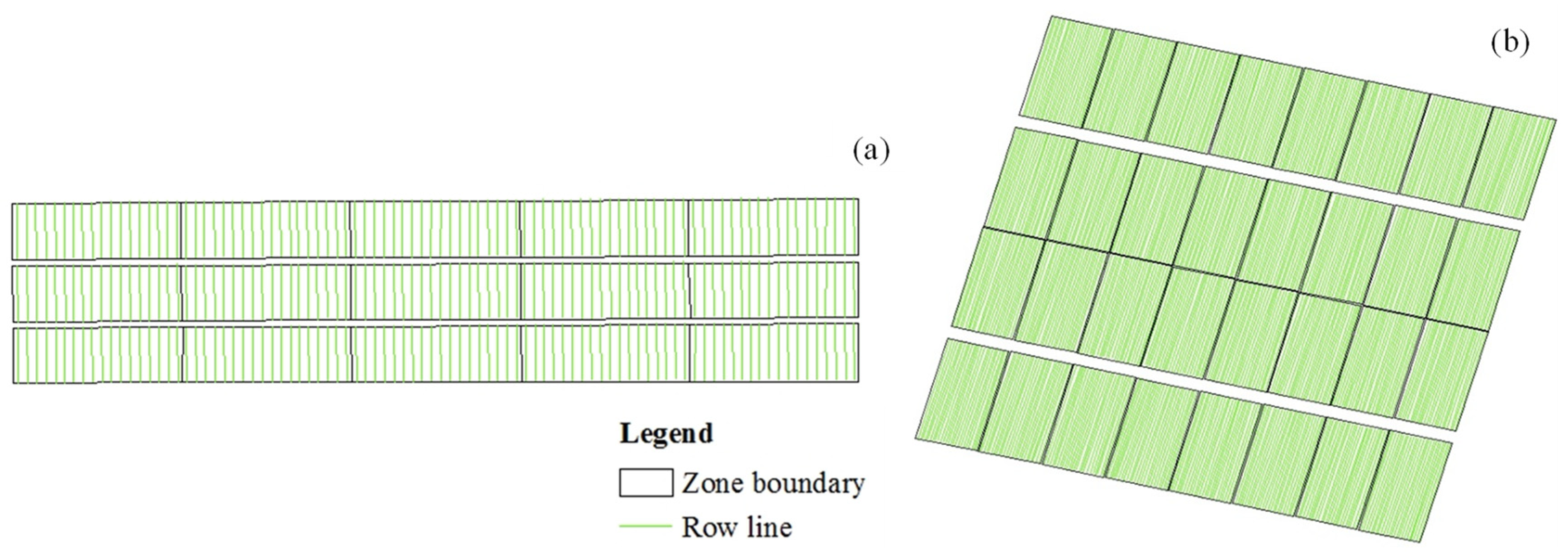
The actual location of cotton and wheat rows was acquired by visual interpretation. During this process, ArcMap (ESRI, Redlands, CA, USA) was used to manually extract the cotton and wheat rows, following the visual interpretation of agronomic experts. The reference crop row line was placed parallel to the row along the centerline of an adjacent inter-row space [20]. The identified rows of cotton and wheat are shown in Figure 2.
2.3. Data Analysis Method
The data analysis consisted of three main phases: (i) vegetation/soil classification; (ii) crop row line identification using different methods; and (iii) evaluation of the performance of different methods for crop row detection. Figure 3 shows the main structure, including the flow chart.
2.3.1. Vegetation/Soil Classification
During UAV image segmentation, the excess green (ExG) index was first calculated using the green, red and blue bands of the original image, with Equations (1)–(4) [27]. The purpose of creating ExG images was to enhance the difference between vegetation and soil. Then, Otsu’s method was used to classify pixels into vegetation pixels and soil pixels, and binary images were produced with “1” representing vegetation and “0” representing soil [28,29]. Otsu’s method is a very good autothreshold selection method. The basic idea of Otsu’s method is to select an optimal threshold value to split the gray-level histogram of an image into two parts based on the principle of maximum between-cluster variance and minimum within-cluster variance [29].
where g, r and b are the green, red and blue bands, respectively, of the image.
2.3.2. Crop Row Identification Using Different Methods
Based on the binary images obtained from the above process, a new method was proposed in this study for row detection in orthomosaic UAV images, and it was compared with the commonly used Hough transform method. Notably, we did not compare the new method with the existing least squares-based method with field images, as it is not directly applicable to the orthomosaic UAV images mentioned previously. A detailed description of the methods used in this study is given in the following.
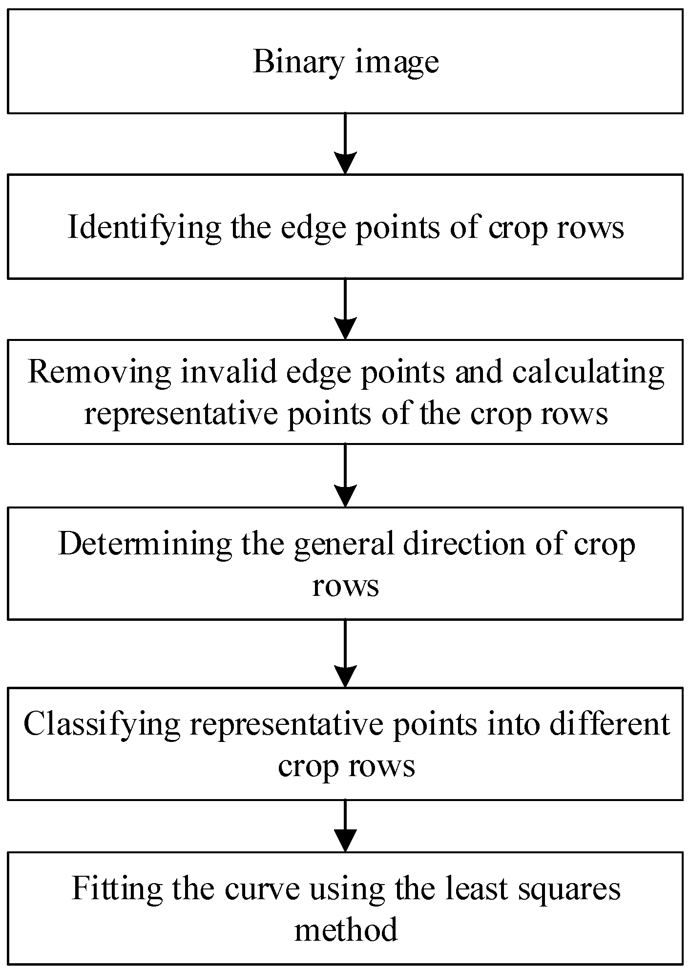
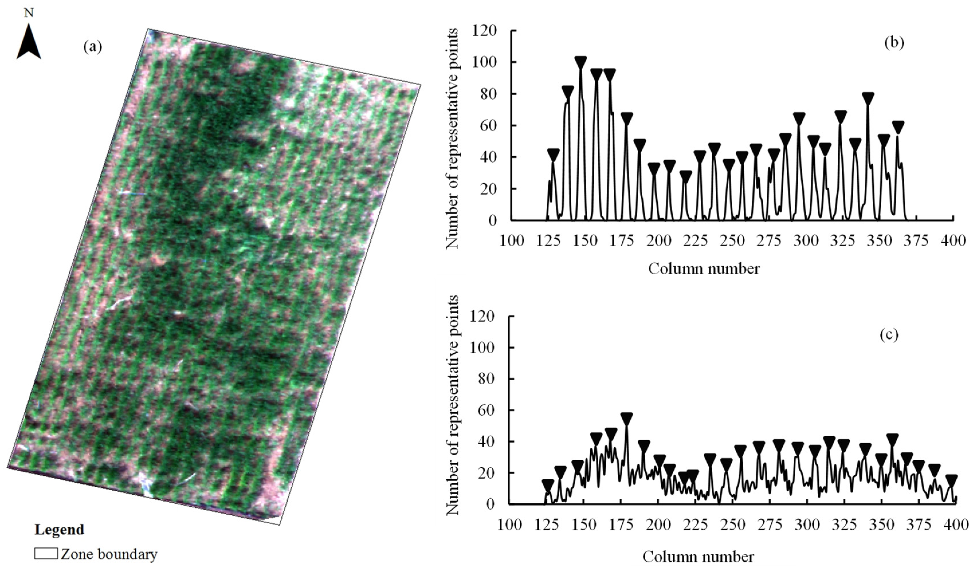
Considering the drawback of the existing least squares-based method for detecting crop rows in UAV images, this research proposes corresponding improvement strategies to form a new method for crop row line identification in orthomosaic UAV images. Because row representative points cannot be obtained by scanning the image row direction when the direction of the crop row is parallel to the image row, this study scans both the image row direction and column direction to obtain the edge points of a crop row, and then a criterion is used to compare the results from them and select the better scan direction. During this process, the standard deviation (SD) of the distance between each pair of edge points is used as the criterion. If the SD of a scanning direction is smaller, it means that the angle between this scanning direction and the crop row in the image is larger than the angle between the other scanning direction and crop row. For example, if the SD value obtained by scanning the row direction of the image is smaller, the angle between the row direction of the crop and the row direction of the image is likely between 45° and 90°. In contrast, if the SD obtained by scanning the row of the image is larger, the angle between the row direction of the crop and the row direction of the image is likely between 0° and 45°. Thus, the edge points obtained from a scanning direction with a smaller SD are more accurate than those from the other direction. Additionally, to avoid an unbearably large calculation caused by the exhaustive method to classify representative points for different crop rows in the existing method, the new method first uses a certain approach to determine the general direction of crop rows. Second, according to this general direction of rows, the image is rotated to make the direction of the crop rows perpendicular to the direction of the image rows. Third, a method is used to determine the approximate position of the crop rows. Finally, based on the determined position, the representative points are classified according to a limiting criterion. It needs to be emphasized that during image rotation, the positions of representative points in the original image are tracked, and then the positions of the selected representative points in the original image are used to fit the crop row line curve using the least square regression method to maintain accuracy. A flow chart of the newly proposed method is shown in Figure 4, and a detailed description of each step is given in the following: (i) Identify the edge points of crop rows. During this process, first, scan the binary image obtained in Section 2.3.1 pixel by pixel by rows and columns and look for mutation points with pixel values from 0 to 1 and from 1 to 0, considering them as left and right edge points for each crop row. Second, calculate the SD of the distance between each pair of edge points obtained by scanning rows and columns. Third, compare the SD values from the scanned rows and columns and retain only the edge points obtained using the scanning direction with smaller SD values. (ii) Remove invalid edge points and calculate representative points of the crop rows. During this process, pairs of edge points with a distance less than 3 pixels and greater than times the crop seeding row spacing are first removed, and then the midpoints of the remaining pairs of edge points are taken as the representative points for each crop row. Because the distance between the paired edge points cannot be greater than times the crop seeding row spacing considering the angle between the selected scanning direction in step (i) and the direction of the crop row, the distance also must not be too small, as a small distance may be a boundary of weeds. (iii) Determine the general direction of rows. During this process, the image is rotated from 0° to 180° with an interval of 0.1°. For every rotation, the number of representative points in the column direction of the image is counted, and a statistical chart is created, with the column number as the x-axis and the number of representative points as the y-axis (Figure 5). Then, the average value of the peak height (AVPH) in the chart is calculated. Through a comparison of the AVPH for every rotation, the rotation angle of the image with the largest AVPH is considered the general direction of crop rows in the UAV image. (iv) Classify representative points into different rows. During this step, the image of representative points is first rotated to make the direction of the crop rows perpendicular to the direction of the image rows according to the angle determined in the previous step. Second, the number of representative points in the column direction is counted, and a statistical chart is created with the column number as the x-axis and the number of representative points as the y-axis. Third, all representative points between 0.375 times the crop seeding row spacing on the left and right of the column where the peak point is located in the statistical graph are regarded as the representative points of the row in that column and indicate the representative points for each row. The crop rows are not completely parallel to each other, resulting in some crop rows having a certain inclination after image rotation. Thus, the representative crop row points for each crop row cannot be well classified using the value of the crop seeding row spacing. We tested many values (the seeding row spacing, 0.75 times the seeding row spacing and 0.5 times the seeding row spacing). Among them, 0.75 times the seeding row spacing was the best value. Therefore, 0.375 times the seeding crop row spacing on the left and right of the approximate position of the row is used herein. Finally, the position of the marked representative points in the original orthomosaic UAV image is tracked. (v) Fit the curve based on the least squares fitting method to represent each row using the representative points of that row in the original image. In this study, because the cotton and wheat rows were nearly linear, a linear fit was used.
As stated previously, many different forms of the Hough transform-based method exist. A common way to enhance computational efficiency is to calculate the representative points of crop rows first and then to apply the Hough transform to the representative points to identify crop rows instead of directly applying the Hough transform to binary images [16]. This approach was adopted in this study. For comparison with the newly proposed method, the method used to identify representative points in the previous section was also used in the Hough transform-based method in this study. In addition, to improve the effectiveness with which the peak points are identified in the parameter space during the Hough transform, the following principles were used: (i) In the parameter space, only the peak points in the range plus or minus 5° of the determined general direction of rows were considered. During this process, the methods used in the previous section for determining the general direction of rows were also used. (ii) Once a peak point in the parameter space was determined, it was not used to detect other peak points within the range of 0.75 times the seeding crop row spacing.
2.3.3. Evaluation of the Crop Row Detection Accuracy for Different Methods
A parameter named the crop row detection accuracy (CRDA), proposed by Vidović et al. [30], is used herein to evaluate the performance of the different crop row detection methods. The CRDA can be regarded as a comprehensive indicator, taking into account both the recall and distance error. The recall is calculated as a percentage based on the number of accurately retrieved lines relative to the total number of actual crop lines. The CRDA was computed by matching the horizontal coordinates () for each crop row obtained by each method under evaluation to the corresponding ground-truth values () according to Equations (5) and (6) [31]. The value of the CRDA ranges from 0 to 1, with values close to 1 indicating good performance. During the comparison, different scenarios for crop row detection were established according to the crop type and field experimental treatment (nitrogen and water levels). In each scenario, a paired t-test was used to compare the performances of the different methods.
where N is the number of crop rows to detect and M is the number of image rows.
where σ is a user-defined parameter, and is set as 0.25 herein, which is higher than the value set by Vidović et al. [30], considering that the difficulty of identifying crop rows in UAV images is greater than that of crop row identification in field images; d is the seeding crop row space in pixels.
3. Results
3.1. Wheat and Cotton Rows in Different Scenarios
Cotton and wheat have different leaf shapes, canopy structures, planting densities and row spacings. Compared with wheat rows in the jointing growth stage, cotton rows are easier to identify in the peak square stage. Because cotton has large leaves and row spacings and is planted in soil covered by mulch, the contrast between the green cotton plants and the soil background is obvious. Thus, the cotton rows could be clearly identified in all nitrogen treatments by visual interpretation (Figure 6). In contrast, wheat has small leaves and row spacings with a high planting density; hence, it is relatively difficult to identify wheat rows, especially when the wheat canopies overlap each other in adjacent rows. For the wheat field experiment, the analysis of variance (ANOVA) method was used to investigate the effect of water and nitrogen on wheat biomass (data are not shown for clarity). The results show that the amount of applied nitrogen had a significant effect on the canopy size of wheat, while the amount of irrigation did not have a significant effect on the canopy size. As the amount of fertilizer was increased, the overlap of the wheat canopy between rows increased, making it generally more difficult to visually identify wheat rows (Figure 7).
3.2. Results of Cotton Row Detection
Based on the use of the ExG index to enhance the difference between vegetation and soil, Otsu’s method was used to automatically segment an image into vegetation and soil. An example of the segmentation results is shown in Figure 8, with a cotton plot image (Figure 8a) and the corresponding vegetation/soil binary image (Figure 8b). The method used in this study can well classify the vegetation pixels and soil pixels in cotton fields. Furthermore, based on the vegetation/soil binary image, the representative points of cotton rows were determined using the method proposed in this study, an example of which is shown in Figure 8c. Many effective points were extracted for each cotton row, and they can indicate the cotton row position very well, which indicates that the method proposed in this study is effective for extracting the representative points of cotton.
For cotton row detection, both the newly proposed method and the Hough transform-based method performed well, with all CRDA values being higher than 0.93. An example of cotton row lines detected by the newly proposed method (red line) and by the Hough transform-based method (blue line) is shown in Figure 9. For different nitrogen scenarios, the CRDA values of the newly proposed method and Hough transform-based method were between 0.99 and 1.00 and between 0.93 and 0.98, respectively. There was no significant difference (p > 0.05) in the CRDA values for either tested method with respect to the different nitrogen scenarios. This may be because the cotton rows were easily identified in all nitrogen treatments in our experiment. A comparison of the newly proposed method with the Hough transform-based method indicated that the CRDA values of the newly proposed method were higher than those of the Hough transform-based method (Figure 10). According to the paired t-test of the CRDA value for each scenario, the newly proposed method performed significantly (p < 0.05) better than the Hough transform-based method, except for the 0 kg/ha nitrogen treatment.
3.3. Results of Wheat Row Detection
An example of a vegetation/soil binary image of wheat is shown in Figure 11b. Using the ExG index and Otsu’s method, we can also well classify the vegetation pixels and soil pixels in wheat fields. Furthermore, based on the vegetation/soil binary image, the representative points of wheat rows were determined, an example of which is shown in Figure 11c. For wheat, when the canopies of adjacent rows overlapped with each other, very few representative row points were extracted. In contrast, when the canopies of adjacent rows were separate from each other, many representative row points were extracted. This indicates that the method used in this study for representative point extraction is suitable for scenarios in which the canopies of adjacent crop rows does not overlap. Actually, when the canopies of field crops are closed, any method used for the representative row point extraction is invalid. Crop row line detection should be performed before the crop canopy closes.
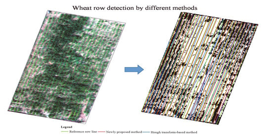
For wheat row detection, the results for both the newly proposed method and the Hough transform-based method were not as good as those for cotton. This may be because wheat has a small row spacing and because leaves from different rows sometimes overlap with each other, which make it difficult to extract enough effective wheat row representative points and then to distinguish each row. An example of wheat row lines detected by the newly proposed method (red line) and by the Hough transform-based method (blue line) is shown in Figure 12. The difference between the row lines detected by the newly proposed method and the reference lines (green line) is much smaller than the difference between the row lines detected by the Hough transform-based method and the reference row lines. In particular, the Hough transform-based method detected many erroneous row lines that were not parallel to the crop row (Figure 12).
For different nitrogen and water scenarios, the CRDA values of the newly proposed method and Hough transform-based method were between 0.66 and 0.82 and between 0.31 and 0.53, respectively. A comparison of the different water level scenarios under the same nitrogen level indicated that there was no significant difference (p > 0.05) in the CRDA values for both tested methods. A comparison of the different nitrogen level scenarios under the same water level indicated that there was also no significant difference (p > 0.05) in the CRDA values for both tested methods. However, the CRDA value tended to decrease with increasing nitrogen fertilizer (Figure 13). This may be because crops grow better under higher nitrogen levels, and the soil between the rows is most likely covered by the wheat canopy, which makes the distinction between the rows more difficult. A comparison of the newly proposed method with the Hough transform-based method indicated that the CRDA values for the newly proposed method were higher than those for the Hough transform-based method (Figure 13). According to the paired t-test of the CRDA value in each scenario, the newly proposed method performed significantly (p < 0.05) better than the Hough transform-based method. The newly proposed method seemed to produce satisfactory results for wheat row detection, in contrast to the Hough transform-based method.
4. Discussion
4.1. Advantages of the Proposed Method over Previous Crop Planting Row Detection Methods
As mentioned previously, the Hough transform-based method has been the most commonly used method for row detection in UAV images until recently. In this study, a method based on a least squares fitting strategy was proposed for crop row detection, and it was compared with the Hough transform-based method. Based on the results, i.e., the peak square growth stage of cotton with large row spacing and clear identification between rows, both the newly proposed method and the Hough transform-based method achieved good results in automatic row detection. However, at the jointing growth stage of wheat, where the row spacings are small and the identification between rows is not very clear, the Hough transform-based method performed much worse than the newly proposed method. This is because when the crop canopies of different rows overlap, fewer representative points of rows were automatically identified. If the representative points of a row are sparse, the Hough transform-based method may detect additional erroneous row lines that are not parallel to the crop rows [18]. The method proposed in this study has the ability to tolerate a certain degree of overlap phenomena from the canopies of adjacent rows when detecting crop rows. Thus, the proposed method is better than the Hough transform-based method.
Tenhunen et al. [18] proposed a method using a least square fitting-based strategy to detect cereal rows. However, their method tests only single UAV images without considering orthomosaics. As these authors stated, their method was limited to finding nearly parallel, roughly straight rows of plants occurring in a window with a restricted size. In this study, we designed a row detection method for application to orthomosaic UAV images. The orthomosaic images eliminate image distortion and offer accurate spatial positions, which can be directly applied to precision agriculture management. The proposed method performed well for cotton and wheat row detection in orthomosaic images of the whole study area. In addition, to identify edge points of rows, two scanning directions were adopted in our method and compared to select the better one, considering that the method can be suitable for detecting rows in any direction in an image. Tenhunen et al. [18] also stated that the row direction in an image is a factor that influences the success of the whole recognition process.
4.2. Comparison of Crop Row Detection Results with Those of Other Studies Using UAV Images
Considering crop row detection results from other studies using UAV images, Su et al. designed a Hough transform-based method for corn row detection, and their best results had a precision between 95.45% and 100.00% for corn in different growth stages when RGB images were used with a spatial resolution of 0.60 cm and a corn row spacing of 60 cm [16]. Precision is the percentage of accurately retrieved crop rows to the total number of retrieved rows. Bah et al. combined a convolutional neural network and the Hough transform to retrieve beet rows in RGB images with a row spacing of 50 cm and an image spatial resolution of approximately 1 cm, and they presented a mean recall value of 0.70 and a mean precision value of 0.90 [32]. In this study, we used the CRDA value to evaluate the performance of different methods for crop row detection. As mentioned previously, the CRDA is a comprehensive parameter considering both the recall and distance error and is better than other evaluation parameters [30,31]. However, because it is a newly proposed parameter, many existing studies have not used it for method evaluation. To compare with other studies, we also calculated the recall and precision. For the cotton experiments with different nitrogen treatments, the newly proposed method in this study obtained recall and precision values of 100%. For the wheat experiments with different nitrogen and water treatments, the newly proposed method obtained recall values between 96.00% and 98.67% and precision values between 89.00% and 98.67%. Compared with those of previous studies, our results seem good.
4.3. Application of the Newly Proposed Method and Future Work
In this study, the newly proposed method was adequately tested for crop row detection in orthomosaic UAV images using two kinds of crops with different canopy structures. Information about the location of crop rows recognized by the method has great potential to be used to further assist in weed identification or to generate accurate field management plots, facilitating precision agricultural production.
In future studies, the proposed method needs to be further tested and modified for crop row detection in images taken under different lighting conditions, as it may not be possible to have clear and cloudless weather conditions for UAV image acquisition during the critical crop management stage. Additionally, different types of sensors, such as digital cameras and multispectral sensors, differ in obtaining spectral information. Based on the spectral information involved, the methods for image segmentation and crop pixel extraction vary. The row detection method proposed in this study uses three bands (blue, green and red), which are commonly included in digital cameras and multispectral sensors. For further study, the method can be modified to include other bands, such as the near-infrared band, which was documented to be suitable for discriminating vegetation and soil.
5. Conclusions
In this study, based on multispectral UAV images of cotton and wheat under different nitrogen and water conditions, a new crop row detection method was proposed and compared with the classical Hough transform-based method using the same image preprocessing strategy for row detection. The proposed method outperformed the Hough transform method in the prediction of both cotton and wheat rows, especially wheat, which has a high density and small row spacings. The method proposed in this study has high potential for use in crop line detection in UAV images, weed detection and the generation of precision management maps. For future research, the proposed method needs to be further tested and modified for crop row detection in images taken under different lighting conditions, and an attempt should be made to use more spectral information for crop pixel segmentation to enhance the accuracy based on multispectral or hyperspectral remote sensing.
Author Contributions
Conceptualization, methodology, writing—original draft preparation, P.C.; data analysis, X.M.; writing—review and editing, F.W. and J.L. All authors have read and agreed to the published version of the manuscript.
Funding
This research was supported by the “National Science and Technology Major Project of China’s High Resolution Earth Observation System, grant number 21-Y20B01-9001-19/22”, “The National Natural Science Foundation of China, grant number 41871344”, and “The Strategic Priority Research Program of the Chinese Academy of Sciences, grant number XDA23100101”.
Acknowledgments
The authors thank Jinran Liu, Zhitao Xu and Yajiao Shi for their valuable assistance during the field campaign.
Conflicts of Interest
The authors declare no conflict of interest.
References
- Arnó, J.; Casasnovas, M.J.A.; Dasi, R.M.; Rosell, J.R. Review. Precision viticulture. Research topics, challenges and opportunities in site-specific vineyard management. Span. J. Agric. Res. 2009, 7, 779–790. [Google Scholar] [CrossRef] [Green Version]
- Balafoutis, A.; Beck, B.; Fountas, S.; Vangeyte, J.; Wal, T.V.D.; Soto, I.; Gómez-Barbero, M.; Barnes, A.; Eory, V. Precision agriculture technologies positively contributing to GHG emissions mitigation, farm productivity and economics. Sustainability 2017, 9, 1339. [Google Scholar] [CrossRef] [Green Version]
- Hedley, C. The role of precision agriculture for improved nutrient management on farms. J. Sci. Food Agric. 2015, 95, 12–19. [Google Scholar] [CrossRef]
- Zhao, C.; Jiang, A.; Huang, W.; Liu, K.; Liu, L.; Wang, J. Evaluation of variable-rate nitrogen recommendation of winter wheat based on SPAD chlorophyll meter measurement. New Zeal. J. Agr. Res. 2007, 50, 735–741. [Google Scholar]
- Mandrini, G.; Bullock, D.S.; Martin, N.F. Modeling the economic and environmental effects of corn nitrogen management strategies in Illinois. Field Crop. Res. 2021, 261, 108000. [Google Scholar] [CrossRef]
- García-Santillán, I.D.; Guerrero, J.M.; Montalvo, M.; Pajares, G. Curved and straight crop row detection by accumulation of green pixels from images in maize fields. Precis. Agric. 2017, 19, 18–41. [Google Scholar] [CrossRef]
- Astrand, B.; Baerveldt, A.J. A vision based row-following system for agricultural field machinery. Mechatronics 2015, 15, 251–269. [Google Scholar] [CrossRef]
- Hague, T.; Tillett, N.D. A bandpass filter-based approach to crop row location and tracking. Mechatronics 2001, 11, 1–12. [Google Scholar] [CrossRef]
- Pang, Y.; Shi, Y.; Gao, S.; Jiang, F.; Veeranampalayam-Sivakumar, A.; Thompson, L.; Luck, J.; Liu, C. Improved crop row detection with deep neural network for early-season maize stand count in UAV imagery. Comput. Electron. Agric. 2020, 178, 105766. [Google Scholar] [CrossRef]
- Zhang, C.; Kovacs, J.M. The application of small unmanned aerial systems for precision agriculture: A review. Precis. Agric. 2012, 13, 693–712. [Google Scholar] [CrossRef]
- Basso, M.; de Freitas, E.P. A UAV guidance system using crop row detection and line follower algorithms. J. Intell. Robot. Syst. 2020, 97, 605–621. [Google Scholar] [CrossRef]
- Hough, P.V.C. Method and Means for Recognizing Complex Patterns. US Patent 306954 18 December 1962. [Google Scholar]
- Duda, R.O.; Hart, P.E. Use of the Hough transformation to detect lines and curves in pictures. Commun. ACM 1972, 15, 11–15. [Google Scholar] [CrossRef]
- Pérez-Ortiz, M.; Peña, J.M.; Gutiérrez, P.A.; Torres-Sánchez, J.; Hervás-Martínez, C.; López-Granados, F. A semi-supervised system for weed mapping in sunflower crops using unmanned aerial vehicles and a crop row detection method. Appl. Soft Comput. 2015, 37, 533–544. [Google Scholar] [CrossRef]
- Weiss, M.; Baret, F. Using 3D point clouds derived from UAV RGB imagery to describe vineyard 3D macro-structure. Remote Sens. 2017, 9, 111. [Google Scholar] [CrossRef] [Green Version]
- Su, W.; Jiang, K.; Yan, A.; Liu, Z.; Zhang, M.; Wang, W. Monitoring of planted lines for breeding corn using UAV remote sensing image. Trans. CSAE 2018, 34, 92–98, (In Chinese with English Abstract). [Google Scholar]
- Basak, J. Learning Hough transform: A neural network model. Neural Comput. 2001, 13, 651–676. [Google Scholar] [CrossRef]
- Tenhunen, H.; Pahikkala, T.; Nevalainen, O.; Teuhola, J.; Mattila, H.; Tyystjärvi, E. Automatic detection of cereal rows by means of pattern recognition techniques. Comput. Electron. Agric. 2019, 162, 677–688. [Google Scholar] [CrossRef]
- Billingsley, J.; Schoenfisch, M. The successful development of a vision guidance system for agriculture. Comput. Electron. Agric. 1997, 16, 147–163. [Google Scholar] [CrossRef]
- Søgaard, H.T.; Olsen, H.J. Determination of crop rows by image analysis without segmentation. Comput. Electron. Agric. 2003, 38, 141–158. [Google Scholar] [CrossRef]
- Montalvo, M.; Pajares, G.; Guerrero, J.M.; Romeo, J.; Guijarro, M.; Ribeiro, A.; Ruz, J.J.; Cruz, J.M. Automatic detection of crop rows in maize fields with high weeds pressure. Expert Syst. Appl. 2012, 39, 11889–11897. [Google Scholar] [CrossRef] [Green Version]
- Jiang, G.; Wang, Z.; Liu, H. Automatic detection of crop rows based on multi-ROIs. Expert Syst. Appl. 2015, 42, 2429–2441. [Google Scholar] [CrossRef]
- Chen, P.; Wang, F. New textural indicators for assessing above-ground cotton biomass extracted from optical imagery obtained via unmanned aerial vehicle. Remote Sens. 2020, 12, 4170. [Google Scholar] [CrossRef]
- Pilon, C. Physiological Responses of Cotton Genotypes to Water-Deficit Stress during Reproductive Development. Ph.D. Thesis, University of Arkansas, Fayetteville, AR, USA, 2015. [Google Scholar]
- Zhao, C.; Chen, P.; Huang, W.; Wang, J.; Wang, Z.; Jiang, A. Effects of two kinds of variable-rate nitrogen application strategies on the production of winter wheat (Triticum aestivum). N. Z. J. Crop. Hortic. Sci. 2009, 37, 149–155. [Google Scholar] [CrossRef]
- Olson, D.; Chatterjee, A.; Franzen, D.W.; Day, S.S. Relationship of drone-based vegetation indices with corn and sugarbeet yields. Agron. J. 2019, 11, 2545–2557. [Google Scholar] [CrossRef]
- Pérez-Ortiz, M.; Peña, J.M.; Gutiérrez, P.A.; Torres-Sánchez, J.; Hervás-Martínez, C.; López-Granados, F. Selecting patterns and features for between- and within- crop-row weed mapping using UAV-imagery. Expert Syst. Appl. 2016, 47, 85–94. [Google Scholar] [CrossRef] [Green Version]
- Otsu, N. A threshold selection method from gray-level histograms. IEEE Trans. Syst. Man Cybern. 1975, 11, 23–27. [Google Scholar] [CrossRef] [Green Version]
- Woebbecke, D.M.; Meyer, G.E.; Von Bargen, K.; Mortensen, D.A. Color indices for weed identification under various soil, residue, and lighting conditions. Trans. ASAE 1995, 38, 259–269. [Google Scholar] [CrossRef]
- Vidović, I.; Cupec, R.; Hocenski, Ž. Crop row detection by global energy minimization. Pattern Recognit. 2016, 55, 68–86. [Google Scholar] [CrossRef]
- García-Santillán, I.D.; Montalvo, M.; Guerrero, J.M.; Pajares, G. Automatic detection of curved and straight crop rows from images in maize fields. Biosyst. Eng. 2017, 156, 61–79. [Google Scholar] [CrossRef]
- Bah, M.D.; Hafiane, A.; Canals, A.R. Crownet: Deep network for crop row detection in UAV images. IEEE Access 2020, 8, 5189–5200. [Google Scholar] [CrossRef]
Figure 1.
Location and layout of the cotton field experiment. (a) N1: 0 kg N/ha; N2: 120 kg N/ha; N3: 240 kg N/ha; N4: 360 kg N/ha; and N5: 480 kg N/ha) and the wheat field experiment. (b) W1: 90 mm irrigation; W2: 60 mm irrigation; N1: 0 kg/ha nitrogen fertilizer; N2: 15,000 kg/ha of farmyard manure; N3: 15,000 kg/ha of farmyard manure and 100 kg/ha of nitrogen fertilizer; N4: 15,000 kg/ha of farmyard manure and 200 kg/ha of nitrogen fertilizer; N5: 15,000 kg/ha of farmyard manure and 300 kg/ha of nitrogen fertilizer) with orthomosaic UAV images.

Figure 2.
Visually identified row lines of cotton (a) and wheat (b).

Figure 3.
Main structure and flow chart of the data analysis procedure used in this study.

Figure 4.
Flow chart of the newly proposed method for row identification.

Figure 5.
Number of representative row points for each column of images from one experimental plot of wheat. (a) An image of the wheat plot; (b) image rotated making the direction of crop rows perpendicular to the direction of image rows; and (c) image not rotated making the direction of crop rows perpendicular to the direction of image rows.

Figure 6.
Examples of cotton images under different amounts of nitrogen fertilizer. 0 kg N/ha (a); 120 kg N/ha (b); 240 kg N/ha (c); 360 kg N/ha (d); 480 kg N/ha (e).
Figure 6.
Examples of cotton images under different amounts of nitrogen fertilizer. 0 kg N/ha (a); 120 kg N/ha (b); 240 kg N/ha (c); 360 kg N/ha (d); 480 kg N/ha (e).

Figure 7.
Examples of wheat images under different amounts of nitrogen fertilizer. 0 kg/ha nitrogen fertilizer (a); 15,000 kg/ha of farmyard manure (b); 15,000 kg/ha of farmyard manure and 100 kg/ha of nitrogen fertilizer (c); 15,000 kg/ha of farmyard manure and 200 kg/ha of nitrogen fertilizer (d); 15,000 kg/ha of farmyard manure and 300 kg/ha of nitrogen fertilizer (e).

Figure 8.
An example of a cotton plot image (a) and the corresponding vegetation/soil binary image (b) and a representative row point image (c).
Figure 8.
An example of a cotton plot image (a) and the corresponding vegetation/soil binary image (b) and a representative row point image (c).

Figure 9.
An example of a detected cotton row line based on the newly proposed method and the Hough transform-based method with vegetation/soil binary images as the background.
Figure 9.
An example of a detected cotton row line based on the newly proposed method and the Hough transform-based method with vegetation/soil binary images as the background.

Figure 10.
CRDA values for different methods when detecting cotton rows under different nitrogen scenarios.
Figure 10.
CRDA values for different methods when detecting cotton rows under different nitrogen scenarios.

Figure 11.
An example of a wheat plot image (a) and the corresponding vegetation/soil binary image (b) and representative row point image (c).
Figure 11.
An example of a wheat plot image (a) and the corresponding vegetation/soil binary image (b) and representative row point image (c).

Figure 12.
An example of a wheat row line detected by the newly proposed method and by the Hough transform-based method with vegetation/soil binary images as the background.
Figure 12.
An example of a wheat row line detected by the newly proposed method and by the Hough transform-based method with vegetation/soil binary images as the background.

Figure 13.
CRDA values for different row detection methods when detecting wheat rows in different nitrogen and irrigation treatments.
Figure 13.
CRDA values for different row detection methods when detecting wheat rows in different nitrogen and irrigation treatments.

Publisher’s Note: MDPI stays neutral with regard to jurisdictional claims in published maps and institutional affiliations. |
© 2021 by the authors. Licensee MDPI, Basel, Switzerland. This article is an open access article distributed under the terms and conditions of the Creative Commons Attribution (CC BY) license (https://creativecommons.org/licenses/by/4.0/).
Share and Cite
MDPI and ACS Style
Chen, P.; Ma, X.; Wang, F.; Li, J. A New Method for Crop Row Detection Using Unmanned Aerial Vehicle Images. Remote Sens. 2021, 13, 3526. https://0-doi-org.brum.beds.ac.uk/10.3390/rs13173526
AMA Style
Chen P, Ma X, Wang F, Li J. A New Method for Crop Row Detection Using Unmanned Aerial Vehicle Images. Remote Sensing. 2021; 13(17):3526. https://0-doi-org.brum.beds.ac.uk/10.3390/rs13173526
Chicago/Turabian StyleChen, Pengfei, Xiao Ma, Fangyong Wang, and Jing Li. 2021. "A New Method for Crop Row Detection Using Unmanned Aerial Vehicle Images" Remote Sensing 13, no. 17: 3526. https://0-doi-org.brum.beds.ac.uk/10.3390/rs13173526
Note that from the first issue of 2016, this journal uses article numbers instead of page numbers. See further details here.