
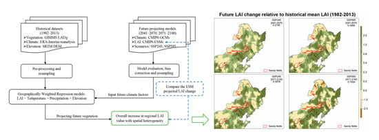
Projecting Future Vegetation Change for Northeast China Using CMIP6 Model


1
School of Geography and Ocean Science, Nanjing University, Nanjing 210023, China
2
Department of Geology and Environmental Geosciences, University of Dayton, Dayton, OH 45469, USA
3
School of Oceanography, Shanghai Jiao Tong University, Shanghai 200240, China
*
Author to whom correspondence should be addressed.
Remote Sens. 2021, 13(17), 3531; https://0-doi-org.brum.beds.ac.uk/10.3390/rs13173531
Submission received: 10 June 2021
/
Revised: 25 August 2021
/
Accepted: 30 August 2021
/
Published: 6 September 2021
Abstract
:Northeast China lies in the transition zone from the humid monsoonal to the arid continental climate, with diverse ecosystems and agricultural land highly susceptible to climate change. This region has experienced significant greening in the past three decades, but future trends remain uncertain. In this study, we provide a quantitative assessment of how vegetation, indicated by the leaf area index (LAI), will change in this region in response to future climate change. Based on the output of eleven CMIP6 global climates, Northeast China is likely to get warmer and wetter in the future, corresponding to an increase in regional LAI. Under the medium emissions scenario (SSP245), the average LAI is expected to increase by 0.27 for the mid-century (2041–2070) and 0.39 for the late century (2071–2100). Under the high emissions scenario (SSP585), the increase is 0.40 for the mid-century and 0.70 for the late century, respectively. Despite the increase in the regional mean, the LAI trend shows significant spatial heterogeneity, with likely decreases for the arid northwest and some sandy fields in this region. Therefore, climate change could pose additional challenges for long-term ecological and economic sustainability. Our findings could provide useful information to local decision makers for developing effective sustainable land management strategies in Northeast China.
1. Introduction
Global climate change can significantly alter vegetation dynamics by modulating key land–atmosphere interactions and other related processes [1]. It has the potential to cause further land degradation, particularly in arid and semi-arid regions [2]. Northeast China (NE China) lies in the transition zone from the humid monsoonal climate in the east to the arid continental climate to the west, with ecosystems highly susceptible to climate change, such as temperate desert steppes and warm shrubs [3]. This region also contains important farm and pastureland supporting the livelihood of hundreds of millions of people. Future climate change is projected to have a large impact on the terrestrial ecosystem in NE China, with significant social and economic consequences [4]. However, how vegetation will respond to future climate change remains uncertain, and detailed studies for projecting future vegetation in this highly vulnerable region are limited. Therefore, the goal of this study is to characterize potential future vegetation changes in NE China in this century.
The greening of terrestrial ecosystems has been reported at both global and regional scales, usually based on long-term satellite-derived vegetation indexes compiled over the past several decades [5,6]. Previous studies have shown a general greening trend since the 1980s in NE China as a result of both a shift toward a warmer and wetter climate and human efforts, such as widespread restoration projects [7,8,9,10]. However, great uncertainties still exist as to whether this greening trend will continue in the future under projected climate change [11,12].
There are two major approaches for projecting future vegetation: direct vegetation output, e.g., leaf area index (LAI), from Earth system models (ESMs) [1], and statistical models using climate output, e.g., temperature and precipitation, from global climate models (GCMs) [13]. The advantage of using ESMs directly to simulate future vegetation is that they have built in biophysical, biogeochemical and carbon cycle processes to account for mechanisms of vegetation change under global warming. However, due to the limited understanding and difficulties in the quantification of many of these processes, there is great uncertainty in ESM-derived LAI projections [14,15]. The statistical approach for projecting future vegetation is based on statistical models built on observed relationships between vegetation and climate drivers. Such statistical models then use the more reliable climate GCM output, such as temperature and precipitation, to derive future vegetation. Although statistical models do not consider mechanisms for vegetation change, they are built upon the observed relationships, and could avoid the uncertainties associated with the poorly constrained parameterizations used in ESM LAI simulations [16]. In addition, statistical models have high spatial resolution, and can reveal detailed local relationships. This approach is commonly used in many previous studies [17,18,19].
Given the limitations of ESM LAI simulations, particularly at the regional level, and their lack of local detail, this study primarily applied a statistical approach to project future vegetation changes (as indicated by LAI) for the study area, a socio-economically important region with ecosystems vulnerable to climate change. It has two specific objectives. First, we developed a statistical model from historical data to quantify the LAI response to climate drivers. Most existing statistical studies use a single model for the entire study area and fail to consider the spatial heterogeneity of correlations between vegetation and climate factors. In this study, we used a local regression technique that accounts for spatial non-stationarity in the relationship. Second, we projected future LAI change based on the statistical model and future climate projections from 11 models in the Coupled Model Intercomparison Project Phase 6 (CMIP6) for both the mid- and late century under two future emissions scenarios. The findings of this study could provide useful information for decision-makers in land and resource management to prevent future land degradation.
2. Materials and Methods
2.1. Study Area
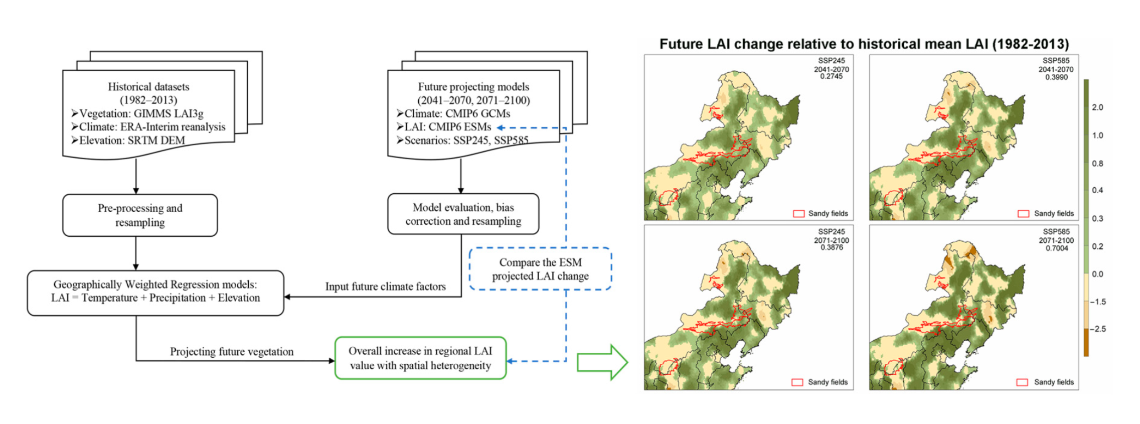
This study focused on NE China, an area within 105–135°E and 35–53.6°N, with an average growing season mean (GSM: May–September) temperature of 21.5 °C and precipitation of 410 mm (Figure 1). It has diverse land cover patterns and ecosystems that are very sensitive to climate change [9,20,21]. This region encompasses the largest agro-pastoral transitional region in China [22], with cropland on the relatively humid east gradually changing into rangeland (grassland) towards the arid west (Figure 1a). It has extensive forest in the mountainous northeast (Figure 1c), as well as the four major sandy fields (Hulunbuir, Horqin, Otindag, and Mu Us) located at the margin of the monsoon region (Figure 1a). The historical GSM LAI from 1982 to 2013 for the entirety of NE China is 1.44 (Figure 1b), ranging from 0.00 to 3.87. These ecosystems provide crucial ecological and economic services for the large population living in the area [23,24]. Therefore, it is very important to establish how future climate change could potentially influence vegetation cover in this region.
2.2. Data
The leaf area index (LAI) is an important vegetation parameter in most ecosystem productivity models and global models of climate, hydrology, and ecology [25]. It is defined as the green leaf area per unit surface area and can be directly derived from satellite images. It has been widely used for monitoring vegetation dynamics under climate change [26,27], because it strongly affects land-surface boundary conditions and the exchange of matter and energy with the atmosphere [28]. In this study, we used the second version of the Global Inventory Modeling and Mapping Studies (GIMMS) LAI3g product derived from the Advanced Very High-Resolution Radiometer (AVHRR). These bi-weekly data cover the period from 1982 to 2013 with a spatial resolution of 1/12 degrees, available at https://0-doi-org.brum.beds.ac.uk/10.3334/ORNLDAAC/1653 (accessed on 18 August 2020). Further details of the AVHRR GIMMS LAI3g product can be found in [29]. It has been widely used to monitor the vegetation dynamic and changes [14,30,31]. Here, we focus on the changes in the mean state between historical and future LAI in the growing season, defined as May to September in NE China.
Historical climate data, including monthly mean temperature and accumulated precipitation, were extracted from the European Centre for Medium-Range Weather Forecasts (ECMWF, https://apps.ecmwf.int/datasets/data/interim-land, accessed on 21 September 2019) ERA-Interim reanalysis dataset with 0.125° spatial resolution for the study area covering 1982–2013 [32]. The reanalysis data were used because of the uneven distribution of meteorological station data and a general lack of stations in the major sandy fields. The ERA-Interim data have been shown to perform well in the study area [33]. Historical climate and LAI data were used to build the regional regression models. In addition, elevation data were extracted from the Shuttle Radar Topography Mission Digital Elevation Model version 3.0 (SRTM30) with a spatial resolution of 90 m (http://glcf.umd.edu/data/srtm, accessed on 1 September 2019).
Future climate projections were obtained from the output of the latest sixth phase of the Coupled Model Inter-comparison Project (CMIP6) climate models (https://esgfnode-.llnl.gov/search/cmip6, accessed on 29 August 2020) [34]. Monthly temperature and precipitation were extracted from 11 climate models (Table A1) for the historical (1982–2013) period, the mid-century (2041–2070) and the late century (2071–2100) under two emissions scenarios (SSP245 and SSP585). The SSP245 and SSP585 scenarios were selected to represent medium and high emissions scenarios, and they are largely comparable to the Representative Concentration Pathway RCP4.5 and RCP8.5 used in CMIP5 [35]. Radiative forcing in the medium and high emissions scenarios peaks at about 4.5 W/m2 (~540 ppm CO2) and 8.5 W/m2 (~940 ppm) in the year 2100, respectively [36]. For comparison with our result, the simulated LAI outputs from 11 Earth System Models (ESMs, Table A2) were also downloaded for both historical and future periods under the SSP245 and SSP585 scenarios. We resampled all datasets to 0.125 degrees for later analysis.
2.3. Methods
2.3.1. Multivariate Regression Analysis
In this study, we first used the multiple linear regression (MLR) method to establish the quantitative relationship between GSM LAI and climate factors (temperature, precipitation) and elevation. The basic MLR can be expressed as follows:
In this model, the dependent variable is the GSM LAI, and independent variables in our model include GSM temperature, precipitation, and elevation. and represent the intercept and slope coefficients for the independent variables separately, and is the random error.
A single regression model could be fitted with all data in the study area by the ordinary least squared (OLS) method, a common approach in many previous studies [18,37]. Such a regression model assumes the LAI–climate relationship to be spatially stationary. However, previous studies suggested large discrepancies in the response of vegetation to climate variation at different locations for different vegetation types and/or densities [9,38,39]. Therefore, a single global model for the entire study area could lead to systematic biases in different regions. This was also noted in some previous studies [40,41]. In order to account for the spatial variation of the LAI–climate relationship, we developed local MLR models using the geographically weighted regression (GWR) approach [42].
GWR constructs a separate MLR equation for every location in the dataset, incorporating the dependent and explanatory variables of locations falling within a neighborhood of each target location [17]. The size of the neighborhood is typically determined by a bandwidth that can be set by the user or calculated through some statistical methods such as cross validation or AICc. In this study, we used an adaptive bandwidth of the closest 500 grid points (~3.0% of total data), corresponding to a neighborhood of 250 km in diameter. For our data, we found this size to be a good compromise between using local information to estimate the model and having sufficient variability within the neighborhood to avoid severe local multicollinearity. Within the neighborhood, the data at each point are weighted based on its distance to the target point using a spatial weight function, so that data closer to the target point have more weight than data further away. In this study, a bi-square kernel-function was used to calculate distance weight. GWR generates layers of spatially variable model coefficients. The performance of the GWR models is evaluated by the overall R2, and each local model is evaluated by a local R2.
2.3.2. Climate Model Evaluation and Bias Correction
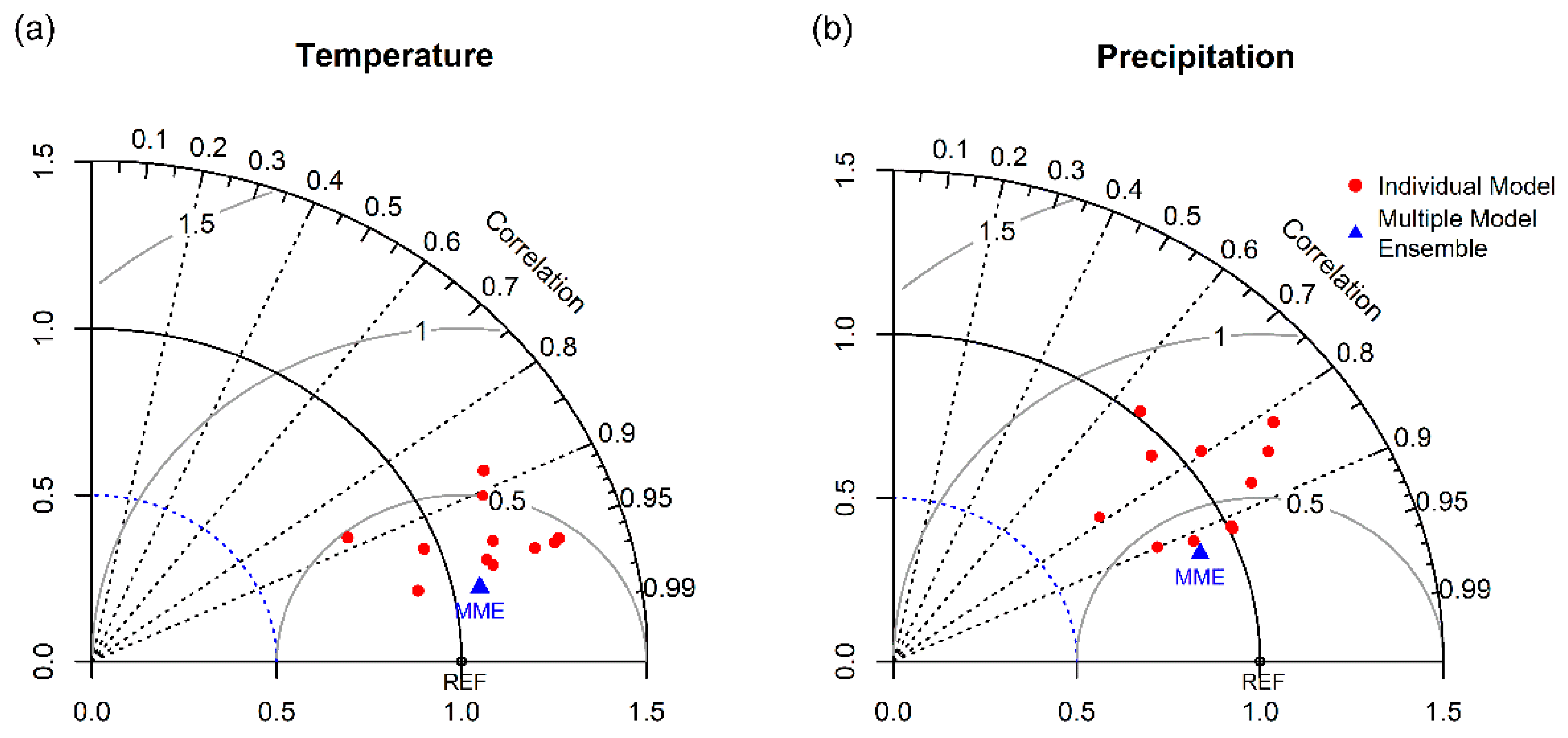
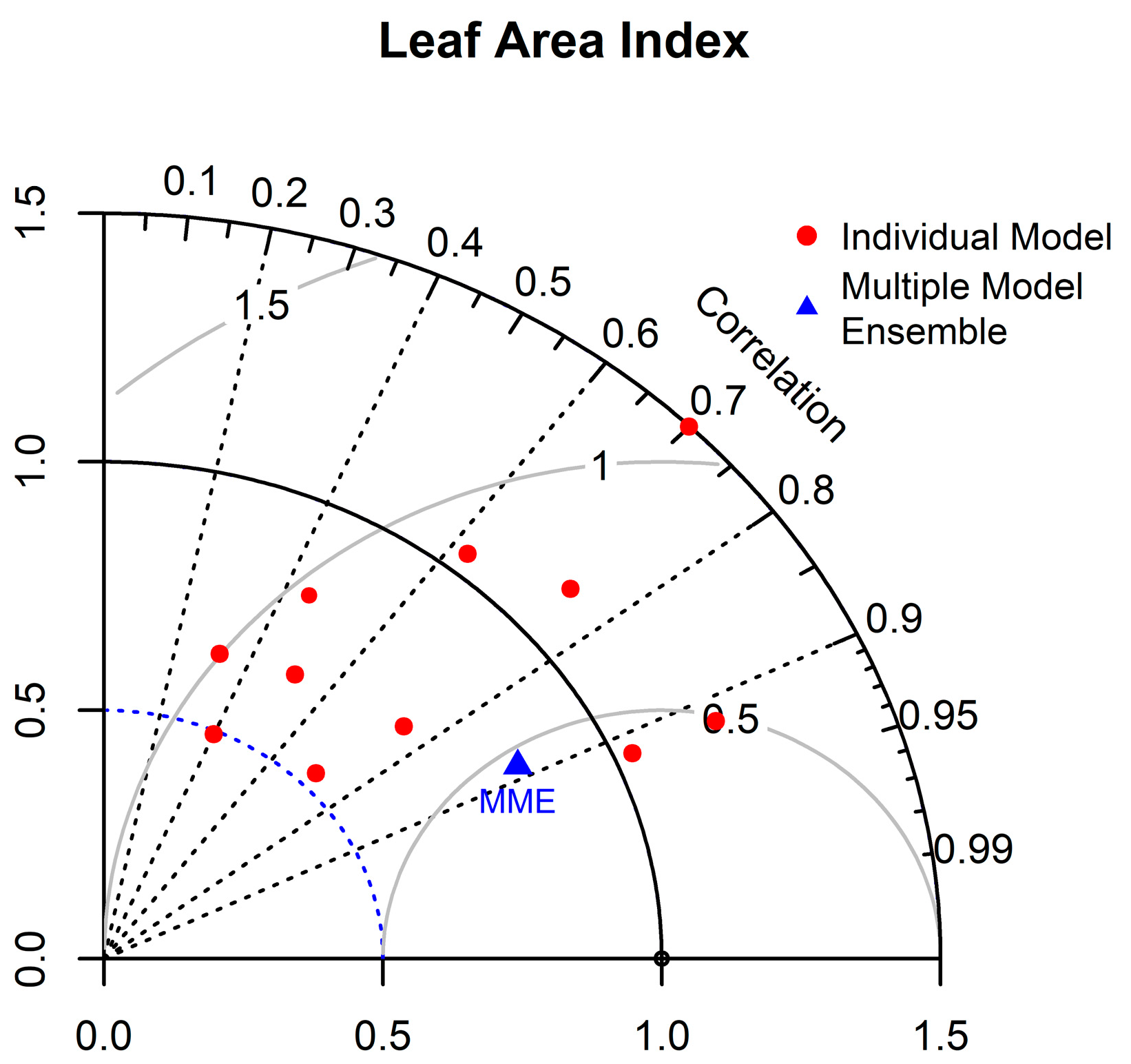
The Taylor diagram was used to examine the performance of CMIP6 climate models in simulating monthly mean temperature and precipitation. The Taylor diagram is a useful visual tool to summarize the degree of similarity between simulated and observed values of a climate field [43,44]. This diagram displays the centered root-mean-square difference (E), the correlation coefficient (r), and the ratio of standard deviations (σ) of a pair of simulated and observed values as a single point on a two-dimensional plot, so that different models can be compared and evaluated [45]. The multiple model ensemble (MME) mean is also calculated for all models. MME has been shown to outperform individual models and is also expected to provide more robust estimates of future changes [46,47].
Due to the uncertainties in model parameterization and calibration, climate model outputs often have significant biases and should not be used directly for future analysis [48,49]. The simplest and widely used method to correct model biases is to adjust the future climate projections by the delta change in the reference period, as follows:
where x is the climate variable from either observed (obs) data or simulated (sim) from climate models for a historical or future period.
3. Results and Discussion
3.1. GWR Model Performance
In order to project future vegetation change in NE China, it is important to first establish an accurate historical quantitative relationship between vegetation and climate drivers [50,51,52,53]. In a previous study, we examined the historical correlation between multiple climate variables and vegetation change, and found that temperature and precipitation are the primary climate drivers for vegetation growth in NE China [9]. However, the exact relationship between vegetation and these climate factors varies based on a variety of factors, such as spatial scale, cover density, and climate conditions [9,39,54]. At the global scale, the rising temperature has extended the growing season and promoted summer photosynthesis in the northern high latitudes while inhibiting vegetation growth in regions where water is limited [39]. Although an increase in precipitation promotes vegetation activity in some arid and semi-arid area [54], it also hinders vegetation growth in wet and cool regions due to insufficient solar radiation [9]. Such spatial heterogeneity of the vegetation–climate relationship is also observed in NE China [55]. Most existing studies used a single global statistical model to describe the entire study region and hence ignored the spatial variation of the relationship [56]. The local geographically weighted regression approach adopted in this study could adapt to the spatial variation of this LAI–climate relationship in NE China.
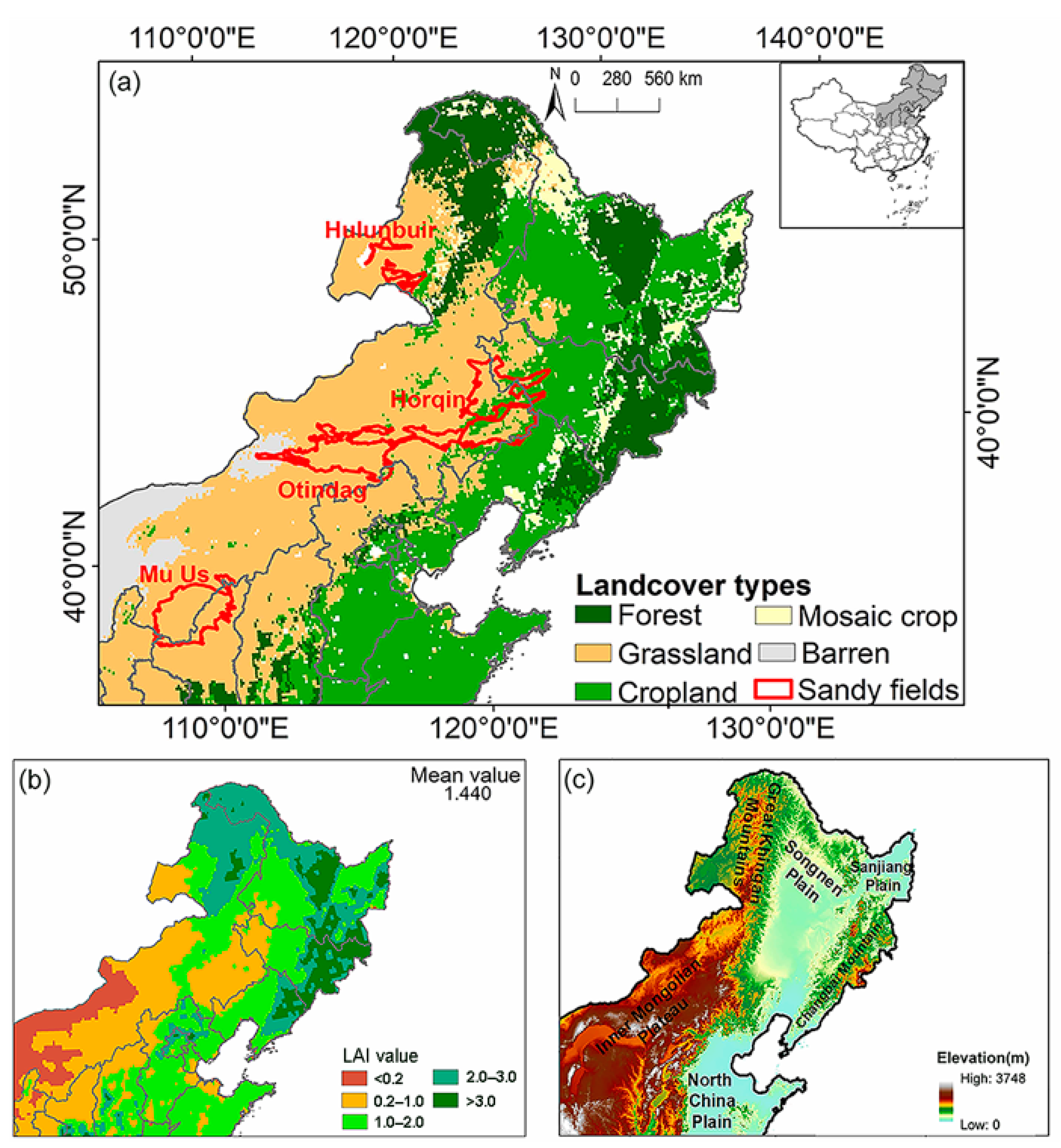
Before implementing GWR modeling, we conducted a single global OLS regression model based on historical GSM data to provide a baseline model performance. The global model performed quite well with a R2 of 0.74, suggesting that the temperature, precipitation and elevation are major controlling factors for the growing season LAI in NE China. However, the model also showed significant spatial clustering of residuals, suggesting systematic biases, owing to the non-stationary vegetation–climate relationship [57]. We then used GWR to fit a separate MLR model for each grid point in NE China, and the results are presented in Figure 2, showing the spatial distribution of local R2 value (Figure 2a), model residual (Figure 2b), and model coefficients for temperature (Figure 2c), precipitation (Figure 2d) and elevation (Figure 2e).
The overall model performance increased significantly with an overall R2 of 0.94, suggesting that the model could account for 94% of the total variance in LAI. The high overall R2 is the result of fitting multiple local regression models to account for the spatial variation of the climate–vegetation relationship. In addition, the spatial distribution of local R2 was used to indicate how well the local regression model fit the observations, and the local models with higher R2 values perform better (Figure 2a). The average local R2 is 0.86, meaning that at each point, GSM temperature, precipitation and elevation could, on average, explain 86% of the variation of GSM LAI within the neighborhood defined by the bandwidth. Overall, 79% of the local R2 values in NE China are greater than 0.8, particularly towards the north and west, areas dominated by natural vegetation less affected by human activities. The local R2 is, in general, high for forest in the northeast (R2 > 0.74), followed by the grassland in the west (R2 > 0.53). Local R2 is lowest in southeast, ranging from 0.38 to 0.67, an area dominated by cropland intensively managed through irrigation and fertilization. Therefore, the results in these areas should be treated with caution.
The model residual is defined as the difference between the observed and predicted LAI values. The global OLS regression model produces residuals that are highly clustered in space, indicating systematic model biases in different regions. Due to its local fitting, GWR not only produces smaller residuals, but also reduces such spatial clustering, leading to more random spatial distribution of residuals. A high level of randomness for model residuals indicates better performance of the regression model [58]. Model residual values are presented in Figure 2b. The areas with a residual larger than 0.5 and smaller than −0.5 only account for 5% for the whole area. In addition, the spatial clustering of model residuals is significantly reduced (Figure 2b), with 56% of pixels having positive residuals and 44% pixels having negative residuals. These results indicate the improved performance of GWR in modeling spatially non-stationary relationships.
The coefficients of temperature range from −1.78 to 4.19, with 62% of the region having negative coefficients for temperature (Figure 2c). The negative values are mostly found in the relatively dry western part of the region, where increasing the temperature could lead to higher evaporation and drier conditions, limiting vegetation growth. The positive coefficients occur more frequently in the relatively humid east, where higher temperature could lead to better thermal conditions and longer sun duration for photosynthesis, hence promoting vegetation growth [59,60].
In contrast to temperature, the coefficients for precipitation are largely positive, ranging from −0.02 to 0.05 (Figure 2d). Overall, 84% of the region has positive values, as more water can relieve drought in the growing season and promote vegetation growth, especially in this transition zonal of semi-arid and semi-humid regions in northern China [9]. The negative coefficients occur mostly in the northern forest region and some cropland regions, where precipitation could lead to a cloudy and cooler environment with reduced sun duration, resulting in negative impacts on vegetation, where growth is more limited by temperature [41,61].
3.2. Future Climatic Change
3.2.1. Climate Model Evaluation
Before projecting future climate change, we first used the Taylor diagram to evaluate the performance of the CMIP6 climate models by comparing their historical simulations with observation. The results are represented in Figure 3 for monthly temperature (Figure 3a) and precipitation (Figure 3b). The results show that the climate models perform well for monthly temperature, as most model simulations are highly correlated with observed values (with most coefficients close to or above 0.9), and have similar standard deviation and an average root-mean-square error (RMSE) of less than half of the standard deviation. For precipitation, the observed and simulated values have correlations mostly greater than 0.8, a similar standard deviation, and RMSEs less than one standard deviation. In both cases, the MME performs better than any individual model. Therefore, MME was used for all following analyses.
3.2.2. Future Changes in Temperature and Precipitation
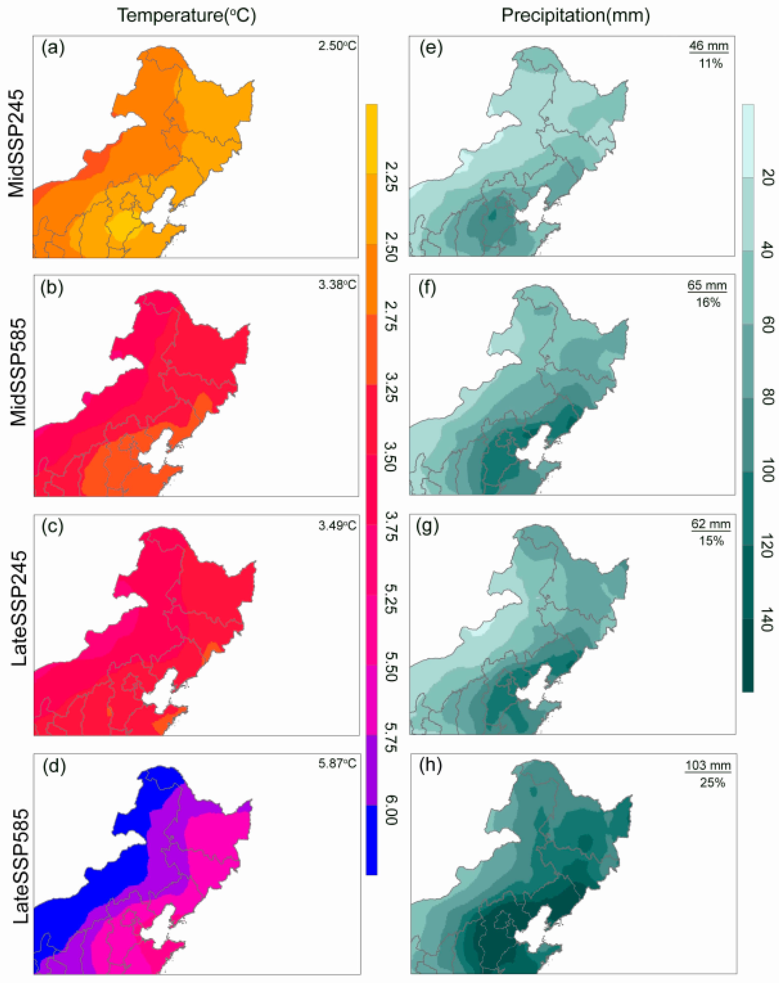
Projected regional mean GSM temperature and precipitation during the mid-century and late century under the SSP245 and SSP585 scenarios are summarized in Table 1 together with the baseline (1982–2013) values. The four different scenarios are labeled as MidSSP245, MidSSP585, LateSSP245, and LateSSP585, respectively. The ranges of values are also provided. Both the regional mean temperature and precipitation are expected to increase, and this increase is greater for the late century and higher emissions scenario. This is consistent with previous projection results based on CMIP5 GCMs [62,63]. For SSP245, the overall temperature for NE China is projected to increase by 2.50 (ranging from 2.20 to 2.86) °C in the mid-century and 3.49 (ranging from 3.19 to 3.87) °C in the late century. For SSP585, the overall temperature is projected to increase by 3.38 (ranging from 3.01 to 3.83) °C in the mid-century and 5.87 (ranging from 5.17 to 6.59) °C in the late century. For SSP245, regional mean precipitation is projected to increase by 46 (ranging from 13 to 102) mm in the mid-century and 62 (ranging from 17 to 124) mm in the late century. For SSP585, it is projected to increase by 65 (ranging from 16 to 125) mm in the mid-century and 103 (ranging from 37 to 192) mm in the late century. These values represent an 11% and 16% increase from 2041 to 2070 and a 15% and 25% increase from 2071 to 2100 under the emissions scenarios SSP245 and SSP585, respectively.
In comparison with the observed temperature range (13.27 °C) of NE China between 1982 and 2013, the range of future temperatures becomes slightly narrower as the emissions scenario increases. For SSP245, the difference between the highest and the lowest value of GSM temperature in the whole region is 13.07 and 13.02 °C for the mid-century and late century, respectively. For SSP585, the range is 12.82 °C and 12.64 °C for the mid-century and late century, respectively. In contrast, the range between the minimum and maximum GSM precipitation increases with time and emissions scenarios. Compared with the observed range of 766 mm, for SSP245, the GSM precipitation range in the entirety of NE China is 808 mm for the mid-century and 838 mm for the late century. For SSP585, the range is projected to be 831 and 875 mm for the mid-century and late century, respectively.
The spatial distribution of the future changes for GSM temperature and precipitation relative to the baseline (1982–2013) are presented in Figure 4. Despite the differences in magnitudes, different scenarios exhibit similar spatial patterns for changes in temperature and precipitation. Temperature tends to increase more in the west and less in the east, whereas precipitation is projected to increase more in the relatively humid east and southeast, and less in the semi-arid west. This largely contributes to the increasing range of GSM precipitation in the region. The spatial variations of climate change will have significant yet differentiated impacts on vegetation growth in NE China.
3.3. Future GSM Vegetation Changes
3.3.1. Future Vegetation Changes Predicted by GWR Models
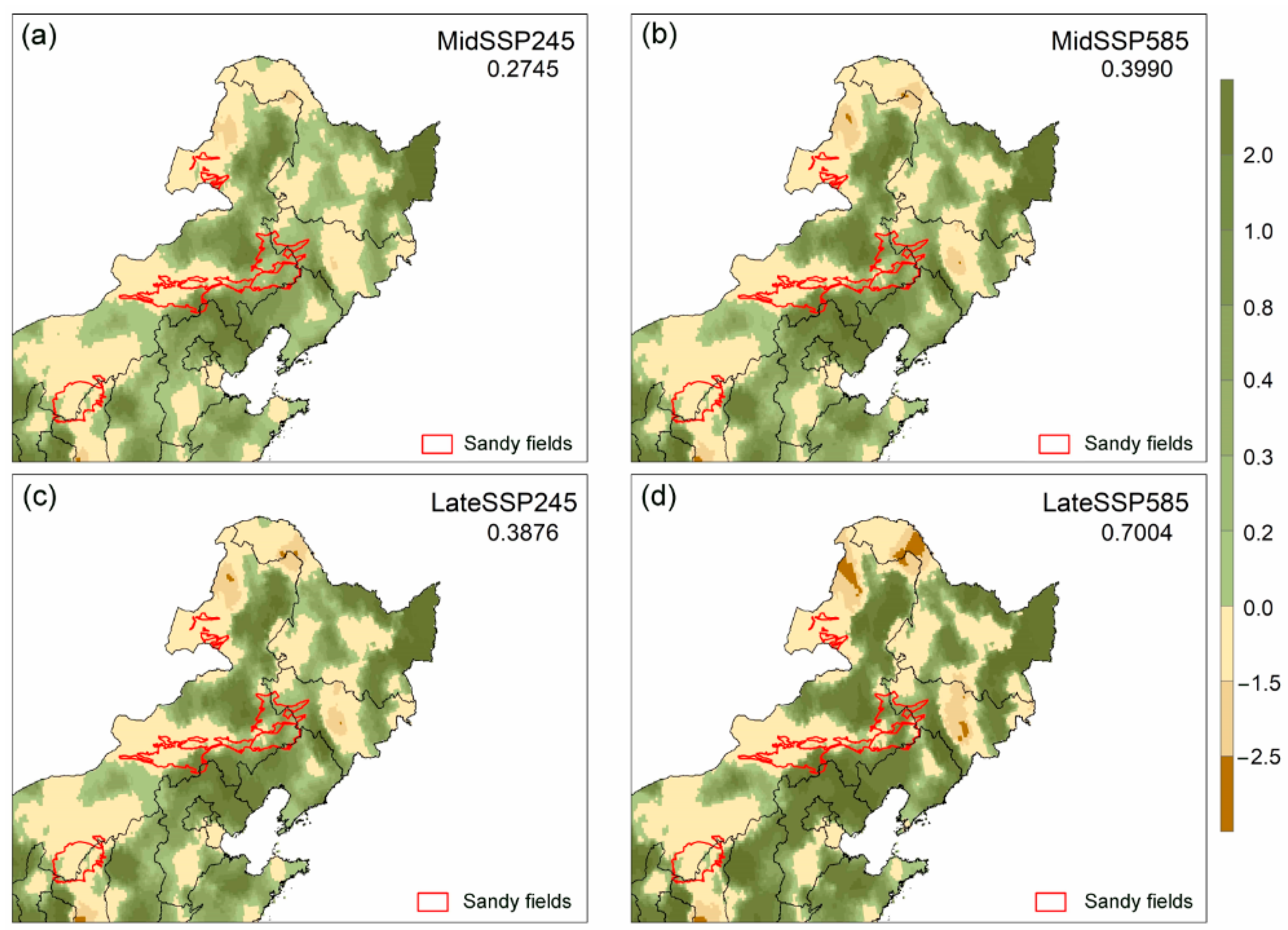
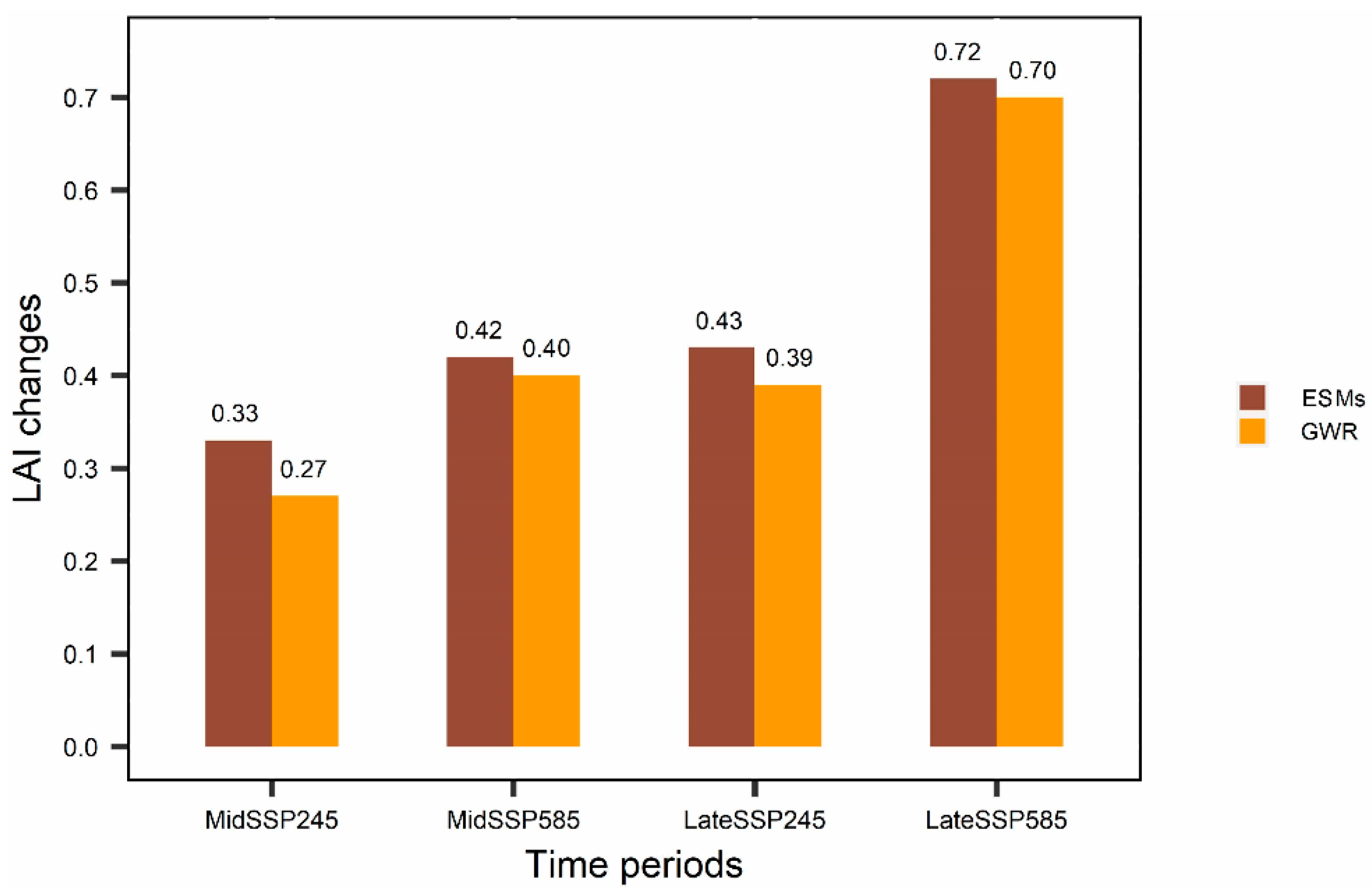
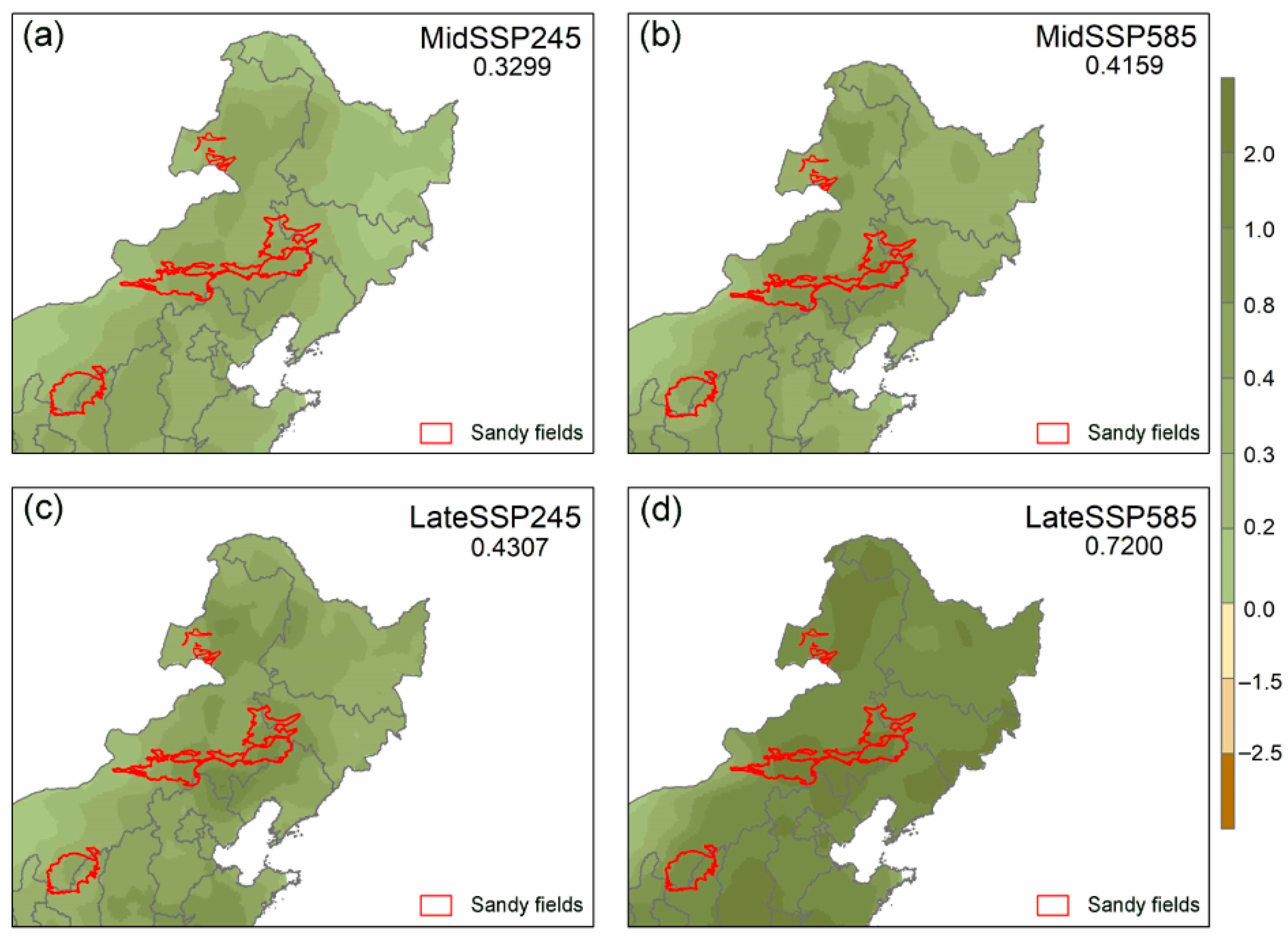
The differences between the historical observed and future projected GSM LAI are presented for MidSPP245, MidSSP585, LateSSP245, and LateSSP585 in Figure 5. Regional mean change values are presented at the upper right corner for each plot. Overall, the GSM LAI in NE China is expected to increase throughout this century. However, the magnitudes of increase are dependent on both the future periods and the emissions scenarios. The increase is less for the near term (mid-century) and the lower emissions scenario (SSP245), and tends to rise in the longer term (late century) and the higher emissions scenario (SSP585). At the mid-century, the average GSM LAI in NE China is projected to increase by 0.27 for SSP245 and 0.40 for SSP585. By the late century, the expected GSM LAI increase is about 0.39 for SSP245 and 0.70 for SSP585. These results seem to suggest that the present greening trend is likely to continue in NE China in future, which is similar to the projected vegetation changes in some previous studies [1,64,65].
Despite the overall LAI increase in future scenarios, its spatial distribution is far from even. Figure 5 shows a greater LAI increase in the relatively humid eastern part of the region, where climate models project a greater precipitation increase and a lower temperature increase (Figure 4), as higher temperature could promote vegetation growth with sufficient precipitation in the future. However, LAI is projected to decrease in the largely arid western part of the region, where climate models project a greater temperature increase and a lower precipitation increase. As a result, the future precipitation increase is not enough to offset the negative impacts of increasing temperature, leading to a decline in LAI. In addition, some studies suggest that forests in the northern mountainous area are less adaptable to changes in climate conditions, and are set to decline in the future, based on ecosystem process models [66]. The magnitude for change, both increases and decreases, varies among different time periods and scenarios. These results are largely consistent with recent studies [64,67]. For example, using multiple linear regression and 12 CMIP5 climate models, Zhou et al. [64] predicted an increased NDVI over mainland China in the period of 2020–2100. Spatially, around 37% of China will experience an NDVI decrease, and much of the decrease will occur in NE China under some emissions scenarios. They also reported degraded growing conditions in parts of NE China using the Vegetation Condition Index, largely due to the environmental stress of drought, which is projected to occur more frequently in NE China from 2041 to 2100 [68].
3.3.2. Future LAI Changes in Sandy Fields
There are four major sandy fields in the transition zone from the humid east to the arid west (Figure 1a), surrounded by intensively used agricultural land with a mixture of pasture and crops. During the past few decades, the areas have been subjected to intensive land management measures to increase vegetation cover and prevent desertification [69,70,71]. Previous studies have shown that whereas the overall effectiveness of these measures remains uncertain, they were more likely to succeed under favorable climate conditions [72,73].
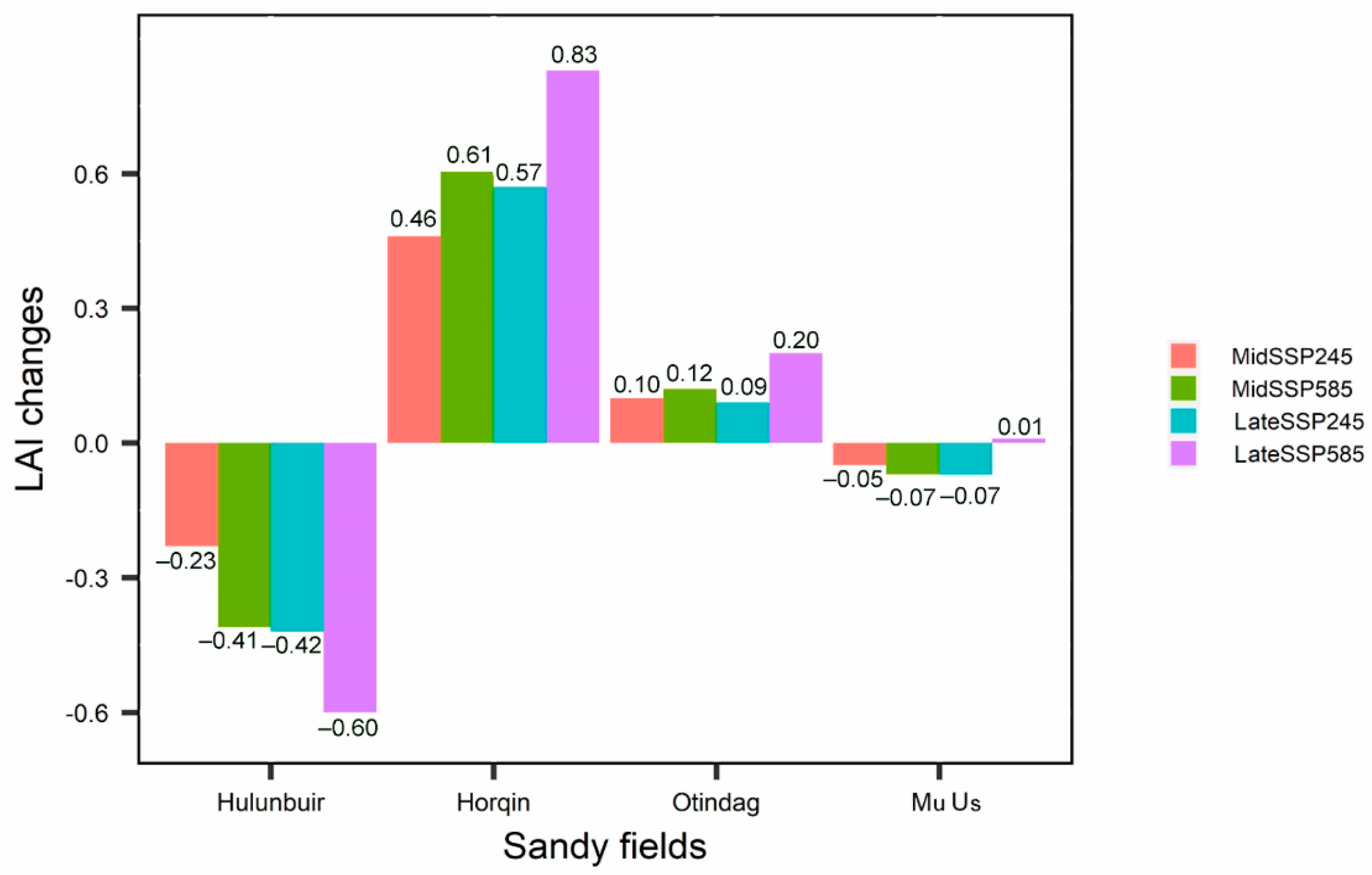
We summarized the LAI changes for the four major sandy fields (Figure 6) to examine their future vulnerability to desertification. Among them, Horqin, located furthest to the east, is likely to experience a significant increase in LAI, especially under the higher emissions scenario and in the longer term (LateSSP585). The GSM LAI in Horqin is expected to increase by 0.46 and 0.57 for the mid- and late-century under SSP245, and by 0.61 and 0.83 for the mid- and late-century under SSP585. The other three sandy fields are located further to the west, along the margin of the monsoon reach. Otindag is likely to see a small LAI increase. Mu Us, on the other hand, is likely to experience a small decrease in the GSM LAI. The largest decrease will occur in Hulunbuir, and the decrease is more significant for the higher emissions scenario in the longer term. This spatial pattern suggests that in the relatively arid west, the benefits of a moderate increase in precipitation on vegetation could be offset by a significant increase in temperature. Therefore, future climate change is likely to cause further land degradation in some of these sandy fields, and will pose additional challenges for land management in areas where desertification remains a long-term threat to the livelihoods of millions of people.
3.3.3. Comparison with ESMs LAI Output
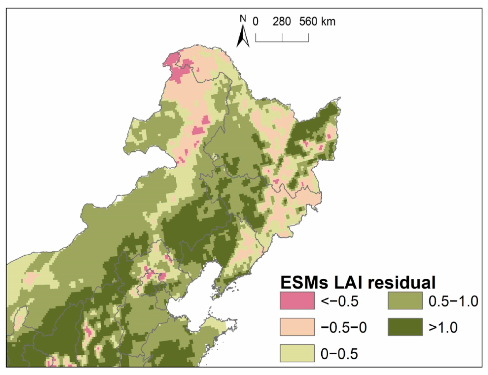
We compared the GWR-based LAI projections with the direct LAI output from 11 CMIP6 ESMs that include the coupled carbon model experiments (Table A2). The Taylor diagram (Figure 7) shows the inferior performance of climate models in simulating LAI in comparison with temperature and precipitation (Figure 3). The correlations between simulated and observed LAI are lower than 0.7 for most models, whereas such correlations are mostly above 0.8 for precipitation and 0.9 for temperature. The RMSEs are mostly between 0.5 and 1 standard deviation. Models tend to underestimate the spatial variation of the LAI, as indicated by the smaller standard deviation of the simulated LAI than that of the observed LAI. As with temperature and precipitation, the MME outperformed all individual models, and was used for comparison with the observed LAI. In general, ESMs tend to overestimate LAI. The regional average LAI is 2.10 for the simulated MME, in comparison to 1.44 for the observed values. Spatially, the climate model MME overestimates LAI in most (85%) of the study region, except for the forested area in the north and northeast (Figure A1). In addition, during the same historical period (1982–2013), almost all models showed a uniform increase in LAI in the entirety of the study area, whereas our previous study found a decreasing trend in about one third of the study region [9]. Based on the assessment of historical LAI simulations, ESMs tend to overestimate LAI and LAI increase in the study area.
CMIP6 ESMs project a nearly uniform increase for all future periods and emissions scenarios (Figure 8 and Figure 9). The overall LAI increases are, in general, consistent with our GWR projections (Figure 8), with a greater increase under the higher emissions scenario and for the late century. In terms of the magnitude of overall LAI change values, ESMs project a slightly higher increase than GWR model results, similar to the overestimation of LAI observed in their historical simulations [29,74]. Previous studies suggest that this is likely caused by the models’ overestimation of physiological response to CO2 fertilization [1]. In fact, the exact effect of CO2 fertilization on vegetation growth remains uncertain, and past assessment varies depending on the attribution approaches and ecosystem models used [11,75,76]. Recently, the dominant global-scale effect of CO2 fertilization has also been questioned [11,12,30,76]. Winkler et al. [30] suggested that the effect of CO2 fertilization is only an important driver of greenness in some biomes, but is not important globally. Regional vegetation cover is often vulnerable to changes in environmental conditions and extreme climate events. By using the fingerprinting method and factorial simulations, Zhu et al. [11] quantified the intersecting contributions of multiple drivers around whole world. They concluded that vegetation increase is likely attributed to factors other than CO2 concentration in areas of intensive ecosystem management, such as NE China. Based on these observations, we believe that the GWR-based method is likely to provide more detailed and realistic future projections.
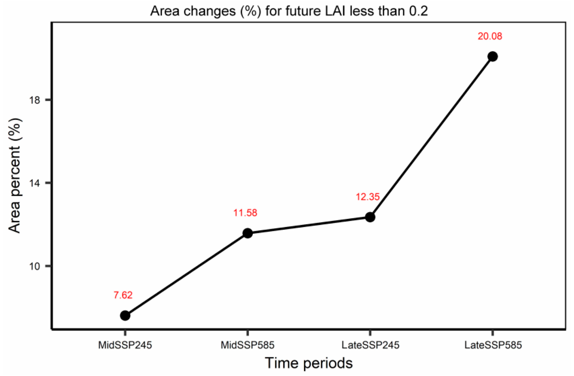
The largest difference between ESMs and GWR projections lies in the spatial variation of future LAI change. Whereas ESMs project an almost uniform LAI increase, the GWR-based results show spatial heterogeneity, with 62–65% of the area showing increasing trends and the rest showing decreasing trends. In addition to ESMs’ propensity to overestimate LAI and LAI increase, this could also be attributed to the low resolution of most ESMs, which range from 100 to 500 km. By comparison, the statistical models are constructed with much more detailed spatial data, and are therefore able to capture local processes and variations. Our projected results show that despite the overall LAI increase, areas with sparse vegetation (LAI < 0.2) are still likely to get larger in all time periods and scenarios (Figure A2). Spatially, arid land, which is concentrated in the southwest at present, is expected to expand northward and eastward under the future climate change conditions (Figure 5). This expansion is more significant for the late century and under the high emissions scenario. This spatial expansion of barren land is likely caused by future climate change for this part of the study region, which is expected to become a lot warmer but only slightly wetter (Figure 4). Therefore, our study suggests that despite an overall vegetation increase, parts of the region are still vulnerable to land degradation in the future, where active land management is necessary to meet the future challenges.
3.4. Research Limitation
We acknowledge several limitations in our study. First, as with all statistical models, we assumed that the observed relationship between vegetation and climate will remain constant in the future. Second, we only used temperature and precipitation to project future vegetation, without considering the other factors such as CO2 fertilization, and nitrogen deposition. However, as we demonstrated above, climate factors are the predominant controls for vegetation in our region, and other factors play at most only minor roles. This is not only supported by other studies [11,64], but also by the high R2 values of our statistical models, which suggest that temperature and precipitation could explain the majority of the variation in vegetation. Third, our model did not include anthropogenic impacts on vegetation, as such impacts are notoriously hard to project for the future. On the one hand, increasing population and economic development could lead to more intensive utilization of land. On the other hand, improved land management could reduce the negative impacts of human activities on vegetation growth. Given such uncertainties, for this study, we assumed that the level of human impact on vegetation (as represented by model residuals) will remain constant in the future. Despite these limitations, we believe that this study contributes to our understanding of climate impacts on vegetation changes in NE China. Compared with future LAI changes projected by multiple CMIP6 ESMs for NE China, our results provide additional spatial details on future vegetation change.
4. Conclusions
In this study, we used the geographically weighted regression to model the spatially non-stationary relationship between LAI and major climate drivers of temperature and precipitation. The model could explain 94% of total variance in LAI over the entirety of NE China, with an average local R2 of 0.86. Coefficients for temperature are mostly negative in the relatively arid west and positive in the humid east, whereas coefficients for precipitation are mostly positive, except in the northern region, where increased precipitation could limit vegetation growth due to shortened sun duration and cooler temperature. Using the ensemble results from multiple CMIP6 models, we then determined future changes in temperature and precipitation for the mid-century (2041–2070) and late century (2071–2100) under the medium (SSP245) and high (SSP585) emissions scenarios. For the entire region, the climate is expected to get warmer and wetter, and the magnitude of such changes is larger for the longer term (late century) and high emissions scenario. Spatially, the arid western part of the region is expected to experience greater temperature increase and lower precipitation increase than the humid eastern part of the region. Combining climate projections and the GWR model, we established future LAI under different future periods and emissions scenarios. Our results show an overall increase in LAI for NE China. This increase is higher for the longer term and under the higher emissions scenario. This suggests that the greening trend observed in recent decades is likely to continue, but this trend is not spatially uniform in NE China. Despite the general increase in LAI, the expansion of arid land is likely to occur in the northwest part of the region, where temperature increase could outpace the precipitation increase. Therefore, land degradation remains a long-term challenge for this region under future climate change conditions.
Author Contributions
Conceptualization, S.-Y.W.; formal analysis, S.-Y.W. and W.Y.; methodology, S.-Y.W. and W.Y.; investigation, S.-Y.W.; writing—original draft preparation, W.Y.; writing—review and editing, S.-Y.W.; supervision, S.-Y.W., Z.X., H.P., H.L.; funding acquisition, S.-Y.W. and S.H. All authors have read and agreed to the published version of the manuscript.
Funding
This research was funded by the National Natural Science Foundation of China, grant number 41830644, 91837102, 41771031, 41871012, and the “333 Project” of Jiangsu Province, grant number BRA 2020030.
Institutional Review Board Statement
Not applicable.
Informed Consent Statement
Not applicable.
Data Availability Statement
The data presented in this study are available from the corresponding website.
Acknowledgments
The authors would like to acknowledge the data provided by Copernicus, the European Centre for Medium-Range Weather Forecasts (ECMWF) and the World Climate Research Programme’s Working Group on Coupled Modelling for leading the CMIP.
Conflicts of Interest
The authors declare no conflict of interest.
Appendix A
Figure A1.
GSM LAI residual simulated by CMIP6 ESMs (multi-model mean), relative to the observed LAI in NE China for 1982–2013.
Figure A1.
GSM LAI residual simulated by CMIP6 ESMs (multi-model mean), relative to the observed LAI in NE China for 1982–2013.

Figure A2.
Change (%) in area with GSM LAI less than 0.2 in NE China under the different emissions scenarios and different time periods. The red number above the point corresponds to the exact area percentage of the entire study region.
Figure A2.
Change (%) in area with GSM LAI less than 0.2 in NE China under the different emissions scenarios and different time periods. The red number above the point corresponds to the exact area percentage of the entire study region.


Table A1.
CMIP6 models used in this study.
| Source ID | Institution ID | Resolution | Country |
|---|---|---|---|
| BCC-CSM2-MR | BCC | 100 KM | China |
| CAMS-CSM1-0 | CAMS | 100 KM | China |
| CanESM5 | CCCma | 500 KM | Canada |
| EC-Earth3 | EC-Earth-Consortium | 100 KM | Europe |
| EC-Earth3-Veg | EC-Earth-Consortium | 100 KM | Europe |
| IPSL-CM6A-LR | IPSL | 250 KM | France |
| MIROC6 | MIROC | 250 KM | Japan |
| MRI-ESM2-0 | MRI | 100 KM | Japan |
| CNRM-CM6-1 | CNRM-CERFACS | 250 KM | France |
| CNRM-ESM2-1 | CNRM-CERFACS | 250 KM | France |
| UKESM1-0-LL | MOHC | 250 KM | UK |
Table A2.
CMIP6 Earth system models (ESMs) used to provide LAI output in this study.
| Source ID | Institution ID | Resolution | Country |
|---|---|---|---|
| ACCESS-ESM1-5 | CSIRO | 250 KM | Australia |
| BCC-CSM2-MR | BCC | 100 KM | China |
| CESM2-WACCM | NCAR | 100 KM | USA |
| CIESM | THU | 100 KM | China |
| CMCC-CM2-SR5 | CMCC | 100 KM | Italy |
| CanESM5 | CCCma | 500 KM | Canada |
| EC-Earth3-Veg | EC-Earth-Consortium | 100 KM | Sweden |
| FIO-ESM-2-0 | FIO-QLNM | 100 KM | China |
| INM-CM5-0 | INM | 100 KM | Russia |
| IPSL-CM6A-LR | IPSL | 250 KM | France |
| MPI-ESM1-2-LR | MPI-M | 250 KM | Germany |
References
- Mahowald, N.; Lo, F.; Zheng, Y.; Harrison, L.; Funk, C.; Lombardozzi, D.; Goodale, C. Projections of Leaf Area Index in Earth System Models. Earth Syst. Dyn. 2016, 7, 211–229. [Google Scholar] [CrossRef] [Green Version]
- UNCCD; UNCBD; UNFCCC. Final report. In Proceedings of the Workshop on Forest and Forest Ecosystems: Promoting Synergy in the Three Rio Conventions, Viterbo, Italy, 5–7 April 2004; pp. 5–7. [Google Scholar]
- Xu, H.; Wang, X.; Zhao, C.; Yang, X. Diverse Responses of Vegetation Growth to Meteorological Drought across Climate Zones and Land Biomes in Northern China from 1981 to 2014. Agric. For. Meteorol. 2018, 262, 1–13. [Google Scholar] [CrossRef]
- Fu, B. Geography: From Knowledge, Science to Decision Making Support. Acta Geogr. Sin. 2017, 72, 1923–1932. [Google Scholar]
- Lamchin, M.; Lee, W.-K.; Jeon, S.W.; Wang, S.W.; Lim, C.H.; Song, C.; Sung, M. Long-Term Trend and Correlation between Vegetation Greenness and Climate Variables in Asia Based on Satellite Data. Sci. Total Environ. 2018, 618, 1089–1095. [Google Scholar] [CrossRef]
- Piao, S.; Wang, X.; Ciais, P.; Zhu, B.; Wang, T.; Liu, J. Changes in Satellite-Derived Vegetation Growth Trend in Temperate and Boreal Eurasia from 1982 to 2006. Glob. Chang. Biol. 2011, 17, 3228–3239. [Google Scholar] [CrossRef]
- Piao, S.; Yin, G.; Tan, J.; Cheng, L.; Huang, M.; Li, Y.; Liu, R.; Mao, J.; Myneni, R.B.; Peng, S.; et al. Detection and Attribution of Vegetation Greening Trend in China over the Last 30 Years. Glob. Chang. Biol. 2015, 21, 1601–1609. [Google Scholar] [CrossRef] [PubMed]
- Liu, D.; Chen, J.; Ouyang, Z. Responses of Landscape Structure to the Ecological Restoration Programs in the Farming-Pastoral Ecotone of Northern China. Sci. Total Environ. 2020, 710, 136311. [Google Scholar] [CrossRef]
- Yuan, W.; Wu, S.-Y.; Hou, S.; Xu, Z.; Lu, H. Normalized Difference Vegetation Index-Based Assessment of Climate Change Impact on Vegetation Growth in the Humid-Arid Transition Zone in Northern China during 1982–2013. Int. J. Climatol. 2019, 39, 5583–5598. [Google Scholar] [CrossRef]
- Lü, Y.; Zhang, L.; Feng, X.; Zeng, Y.; Fu, B.; Yao, X.; Li, J.; Wu, B. Recent Ecological Transitions in China: Greening, Browning and Influential Factors. Sci. Rep. 2015, 5, 1–8. [Google Scholar] [CrossRef]
- Zhu, Z.; Piao, S.; Myneni, R.B.; Huang, M.; Zeng, Z.; Canadell, J.G.; Ciais, P.; Sitch, S.; Friedlingstein, P.; Arneth, A.; et al. Greening of the Earth and Its Drivers. Nat. Clim. Chang. 2016, 6, 791–795. [Google Scholar] [CrossRef]
- Zhao, Q.; Zhu, Z.; Zeng, H.; Zhao, W.; Myneni, R.B. Future Greening of the Earth May Not Be as Large as Previously Predicted. Agric. For. Meteorol. 2020, 292–293, 108111. [Google Scholar] [CrossRef]
- Ouyang, W.; Wan, X.; Xu, Y.; Wang, X.; Lin, C. Vertical Difference of Climate Change Impacts on Vegetation at Temporal-Spatial Scales in the Upper Stream of the Mekong River Basin. Sci. Total Environ. 2020, 701, 134782. [Google Scholar] [CrossRef]
- Anav, A.; Murray-Tortarolo, G.; Friedlingstein, P.; Sitch, S.; Piao, S.; Zhu, Z. Evaluation of Land Surface Models in Reproducing Satellite Derived Leaf Area Index over the High-Latitude Northern Hemisphere. Part II: Earth System Models. Remote Sens. 2013, 5, 3637–3661. [Google Scholar] [CrossRef] [Green Version]
- Ziehn, T.; Lenton, A.; Law, R.M.; Matear, R.J.; Chamberlain, M.A. The Carbon Cycle in the Australian Community Climate and Earth System Simulator (ACCESS-ESM1)—Part 2: Historical Simulations. Geosci. Model Dev. 2017, 10, 2591–2614. [Google Scholar] [CrossRef] [Green Version]
- Shen, M.; Piao, S.; Jeong, S.-J.; Zhou, L.; Zeng, Z.; Ciais, P.; Chen, D.; Huang, M.; Jin, C.-S.; Li, L.Z.X.; et al. Evaporative Cooling over the Tibetan Plateau Induced by Vegetation Growth. Proc. Natl. Acad. Sci. USA 2015, 112, 9299–9304. [Google Scholar] [CrossRef] [PubMed] [Green Version]
- Gao, J.; Jiao, K.; Wu, S.; Ma, D.; Zhao, D.; Yin, Y.; Dai, E. Past and Future Effects of Climate Change on Spatially Heterogeneous Vegetation Activity in China. Earth’s Future 2017, 5, 679–692. [Google Scholar] [CrossRef] [Green Version]
- Han, J.-C.; Huang, Y.; Zhang, H.; Wu, X. Characterization of Elevation and Land Cover Dependent Trends of NDVI Variations in the Hexi Region, Northwest China. J. Environ. Manag. 2019, 232, 1037–1048. [Google Scholar] [CrossRef]
- Jiao, K.; Gao, J.; Liu, Z. Precipitation Drives the NDVI Distribution on the Tibetan Plateau While High Warming Rates May Intensify Its Ecological Droughts. Remote Sens. 2021, 13, 1305. [Google Scholar] [CrossRef]
- Ren, Y.; Yue, P.; Zhang, Q.; Liu, X. Influence of Land Surface Aridification on Regional Monsoon Precipitation in East Asian Summer Monsoon Transition Zone. Theor. Appl. Climatol. 2021, 144, 93–102. [Google Scholar] [CrossRef]
- Jiang, P.; Ding, W.; Yuan, Y.; Ye, W. Diverse Response of Vegetation Growth to Multi-Time-Scale Drought under Different Soil Textures in China’s Pastoral Areas. J. Environ. Manag. 2020, 274, 110992. [Google Scholar] [CrossRef]
- Duan, H.; Yan, C.; Tsunekawa, A.; Song, X.; Li, S.; Xie, J. Assessing Vegetation Dynamics in the Three-North Shelter Forest Region of China Using AVHRR NDVI Data. Environ. Earth Sci. 2011, 64, 1011–1020. [Google Scholar] [CrossRef]
- Cao, S.; Chen, L.; Shankman, D.; Wang, C.; Wang, X.; Zhang, H. Excessive Reliance on Afforestation in China’s Arid and Semi-Arid Regions: Lessons in Ecological Restoration. Earth-Sci. Rev. 2011, 104, 240–245. [Google Scholar] [CrossRef]
- Zhang, G.; Dong, J.; Xiao, X.; Hu, Z.; Sheldon, S. Effectiveness of Ecological Restoration Projects in Horqin Sandy Land, China Based on SPOT-VGT NDVI Data. Ecol. Eng. 2012, 38, 20–29. [Google Scholar] [CrossRef]
- Sellers, P.J. Modeling the Exchanges of Energy, Water, and Carbon Between Continents and the Atmosphere. Science 1997, 275, 502–509. [Google Scholar] [CrossRef] [Green Version]
- Tang, S.; Chen, J.; Zhu, Q.; Li, X.; Chen, M.; Sun, R.; Zhou, Y.; Deng, F.; Xie, D. LAI Inversion Algorithm Based on Directional Reflectance Kernels. J. Environ. Manag. 2007, 85, 638–648. [Google Scholar] [CrossRef]
- Fang, S.; Yan, J.; Che, M.; Zhu, Y.; Liu, Z.; Pei, H.; Zhang, H.; Xu, G.; Lin, X. Climate Change and the Ecological Responses in Xinjiang, China: Model Simulations and Data Analyses. Quat. Int. 2013, 311, 108–116. [Google Scholar] [CrossRef]
- Pielke, R.A.; Avissar, R.; Raupach, M.; Dolman, A.J.; Zeng, X.; Denning, A.S. Interactions between the Atmosphere and Terrestrial Ecosystems: Influence on Weather and Climate. Glob. Chang. Biol. 1998, 4, 461–475. [Google Scholar] [CrossRef]
- Zhu, Z.; Bi, J.; Pan, Y.; Ganguly, S.; Anav, A.; Xu, L.; Samanta, A.; Piao, S.; Nemani, R.R.; Myneni, R.B. Global Data Sets of Vegetation Leaf Area Index (LAI) 3g and Fraction of Photosynthetically Active Radiation (FPAR) 3g Derived from Global Inventory Modeling and Mapping Studies (GIMMS) Normalized Difference Vegetation Index (NDVI3g) for the Period 1981 to 2011. Remote Sens. 2013, 5, 927–948. [Google Scholar]
- Winkler, A.J.; Myneni, R.B.; Hannart, A.; Sitch, S.; Haverd, V.; Lombardozzi, D.; Arora, V.K.; Pongratz, J.; Nabel, J.E.; Goll, D.S.; et al. Slow-down of the Greening Trend in Natural Vegetation with Further Rise in Atmospheric CO2. Earth Space Sci. Open Arch. (ESSOAr) 2020. [Google Scholar] [CrossRef]
- Helbig, M.; Waddington, J.M.; Alekseychik, P.; Amiro, B.D.; Aurela, M.; Barr, A.G.; Black, T.A.; Blanken, P.D.; Carey, S.K.; Chen, J.; et al. Increasing Contribution of Peatlands to Boreal Evapotranspiration in a Warming Climate. Nat. Clim. Chang. 2020, 10, 555–560. [Google Scholar] [CrossRef]
- Berrisford, P.; Dee, D.; Fielding, K.; Fuentes, M.; Kallberg, P.; Kobayashi, S.; Uppala, S. The ERA-Interim Archive. ERA Rep. Ser. 2009, 1, 1–16. [Google Scholar]
- Berrisford, P.; Kaallberg, P.; Kobayashi, S.; Dee, D.; Uppala, S.; Simmons, A.; Poli, P.; Sato, H. Atmospheric Conservation Properties in ERA-Interim. Q. J. R. Meteorol. Soc. 2011, 137, 1381–1399. [Google Scholar] [CrossRef]
- Eyring, V.; Bony, S.; Meehl, G.A.; Senior, C.A.; Stevens, B.; Stouffer, R.J.; Taylor, K.E. Overview of the Coupled Model Intercomparison Project Phase 6 (CMIP6) Experimental Design and Organization. Geosci. Model Dev. 2016, 9, 1937–1958. [Google Scholar] [CrossRef] [Green Version]
- Zampieri, M.; Grizzetti, B.; Meroni, M.; Scoccimarro, E.; Vrieling, A.; Naumann, G.; Toreti, A. Annual Green Water Resources and Vegetation Resilience Indicators: Definitions, Mutual Relationships, and Future Climate Projections. Remote Sens. 2019, 11, 2708. [Google Scholar] [CrossRef] [Green Version]
- Thomas, D.; Knight, M.; Wiggs, G. Remobilization of Southern African Desert Dune Systems by Twenty-First Century Global Warming. Nature 2005, 435, 1218–1221. [Google Scholar] [CrossRef] [PubMed]
- Liu, H.; Jiao, F.; Yin, J.; Li, T.; Gong, H.; Wang, Z.; Lin, Z. Nonlinear Relationship of Vegetation Greening with Nature and Human Factors and Its Forecast–A Case Study of Southwest China. Ecol. Indic. 2020, 111, 106009. [Google Scholar] [CrossRef]
- Chu, H.; Venevsky, S.; Wu, C.; Wang, M. NDVI-Based Vegetation Dynamics and Its Response to Climate Changes at Amur-Heilongjiang River Basin from 1982 to 2015. Sci. Total Environ. 2019, 650, 2051–2062. [Google Scholar] [CrossRef] [PubMed]
- Kawabata, A.; Ichii, K.; Yamaguchi, Y. Global Monitoring of Interannual Changes in Vegetation Activities Using NDVI and Its Relationships to Temperature and Precipitation. Int. J. Remote Sens. 2001, 22, 1377–1382. [Google Scholar] [CrossRef]
- Foody, G. Geographical Weighting as a Further Refinement to Regression Modelling: An Example Focused on the NDVI–Rainfall Relationship. Remote Sens. Environ. 2003, 88, 283–293. [Google Scholar] [CrossRef]
- Zhao, Z.; Gao, J.; Wang, Y.; Liu, J.; Li, S. Exploring Spatially Variable Relationships between NDVI and Climatic Factors in a Transition Zone Using Geographically Weighted Regression. Theor. Appl. Climatol. 2015, 120, 507–519. [Google Scholar] [CrossRef]
- Fotheringham, A.S.; Brunsdon, C.; Charlton, M. Geographically Weighted Regression: The Analysis of Spatially Varying Relationships; John Wiley & Sons: Hoboken, NJ, USA, 2003. [Google Scholar]
- Taylor, K.E. Summarizing Multiple Aspects of Model Performance in a Single Diagram. J. Geophys. Res. Atmos. 2001, 106, 7183–7192. [Google Scholar] [CrossRef]
- Taylor, K.E.; Stouffer, R.J.; Meehl, G.A. An Overview of CMIP5 and the Experiment Design. Bull. Am. Meteorol. Soc. 2012, 93, 485–498. [Google Scholar] [CrossRef] [Green Version]
- Pincus, R.; Batstone, C.P.; Hofmann, R.J.P.; Taylor, K.E.; Glecker, P.J. Evaluating the Present-Day Simulation of Clouds, Precipitation, and Radiation in Climate Models. J. Geophys. Res. Atmos. 2008, 113, D14209. [Google Scholar] [CrossRef]
- Sillmann, J.; Kharin, V.V.; Zwiers, F.; Zhang, X.; Bronaugh, D. Climate Extremes Indices in the CMIP5 Multimodel Ensemble: Part 2. Future Climate Projections. J. Geophys. Res. Atmos. 2013, 118, 2473–2493. [Google Scholar] [CrossRef]
- Toh, Y.Y.; Turner, A.G.; Johnson, S.J.; Holloway, C.E. Maritime Continent Seasonal Climate Biases in AMIP Experiments of the CMIP5 Multimodel Ensemble. Clim. Dyn. 2018, 50, 777–800. [Google Scholar] [CrossRef] [Green Version]
- Lafon, T.; Dadson, S.; Buys, G.; Prudhomme, C. Bias Correction of Daily Precipitation Simulated by a Regional Climate Model: A Comparison of Methods. Int. J. Climatol. 2013, 33, 1367–1381. [Google Scholar] [CrossRef] [Green Version]
- Raty, O.; Räisänen, J.; Ylhäisi, J.S. Evaluation of Delta Change and Bias Correction Methods for Future Daily Precipitation: Intermodel Cross-Validation Using ENSEMBLES Simulations. Clim. Dyn. 2014, 42, 2287–2303. [Google Scholar] [CrossRef]
- Hickler, T.; Eklundh, L.; Seaquist, J.W.; Smith, B.; Ardö, J.; Olsson, L.; Sykes, M.T.; Sjöström, M. Precipitation Controls Sahel Greening Trend. Geophys. Res. Lett. 2005, 32. [Google Scholar] [CrossRef]
- Ichii, K.; Kawabata, A.; Yamaguchi, Y. Global Correlation Analysis for NDVI and Climatic Variables and NDVI Trends: 1982–1990. Int. J. Remote Sens. 2002, 23, 3873–3878. [Google Scholar] [CrossRef]
- Pettorelli, N.; Vik, J.O.; Mysterud, A.; Gaillard, J.-M.; Tucker, C.J.; Stenseth, N.C. Using the Satellite-Derived NDVI to Assess Ecological Responses to Environmental Change. Trends Ecol. Evol. 2005, 20, 503–510. [Google Scholar] [CrossRef]
- Zhang, Y.; Song, C.; Band, L.E.; Sun, G.; Li, J. Reanalysis of Global Terrestrial Vegetation Trends from MODIS Products: Browning or Greening? Remote Sens. Environ. 2017, 191, 145–155. [Google Scholar] [CrossRef] [Green Version]
- Piao, S.; Mohammat, A.; Fang, J.; Cai, Q.; Feng, J. NDVI-Based Increase in Growth of Temperate Grasslands and Its Responses to Climate Changes in China. Glob. Environ. Chang. 2006, 16, 340–348. [Google Scholar] [CrossRef]
- Mason, J.; Lu, H.; Zhou, Y.; Miao, X.; Swinehart, J.; Liu, Z.; Goble, R.; Yi, S. Dune Mobility and Aridity at the Desert Margin of Northern China at a Time of Peak Monsoon Strength. Geology 2009, 37, 947–950. [Google Scholar] [CrossRef]
- Usman, U.; Yelwa, S.; Gulumbe, S.; Danbaba, A.; Nir, R. Modelling Relationship between NDVI and Climatic Variables Using Geographically Weighted Regression. J. Math. Sci. Appl. 2013, 1, 24–28. [Google Scholar]
- Gao, J.; Jiao, K.; Wu, S. Investigating the Spatially Heterogeneous Relationships between Climate Factors and NDVI in China during 1982 to 2013. J. Geogr. Sci. 2019, 29, 1597–1609. [Google Scholar] [CrossRef] [Green Version]
- Legendre, P. Spatial Autocorrelation: Trouble or New Paradigm? Ecology 1993, 74, 1659–1673. [Google Scholar] [CrossRef]
- Bachelet, D.; Neilson, R.P.; Lenihan, J.M.; Drapek, R.J. Climate Change Effects on Vegetation Distribution and Carbon Budget in the United States. Ecosystems 2001, 4, 164–185. [Google Scholar] [CrossRef]
- Wang, M.; Wang, J.; Chen, D.; Duan, A.; Liu, Y.; Zhou, S.; Guo, D.; Wang, H.; Ju, W. Recent Recovery of the Boreal Spring Sensible Heating over the Tibetan Plateau Will Continue in CMIP6 Future Projections. Environ. Res. Lett. 2019, 14, 124066. [Google Scholar] [CrossRef] [Green Version]
- Wei, S.; Yi, C.; Fang, W.; Hendrey, G. A Global Study of GPP Focusing on Light-Use Efficiency in a Random Forest Regression Model. Ecosphere 2017, 8, e01724. [Google Scholar] [CrossRef]
- Wang, L.; Chen, W. A CMIP5 Multimodel Projection of Future Temperature, Precipitation, and Climatological Drought in China. Int. J. Climatol. 2014, 34, 2059–2078. [Google Scholar] [CrossRef]
- Wu, S.-Y.; Wu, Y.; Wen, J. Future Changes in Precipitation Characteristics in China. Int. J. Climatol. 2019, 39, 3558–3573. [Google Scholar] [CrossRef]
- Zhou, Z.; Ding, Y.; Shi, H.; Cai, H.; Fu, Q.; Liu, S.; Li, T. Analysis and Prediction of Vegetation Dynamic Changes in China: Past, Present and Future. Ecol. Indic. 2020, 117, 106642. [Google Scholar] [CrossRef]
- Fu, J.; Liu, J.; Wang, X.; Zhang, M.; Chen, W.; Chen, B. Ecological Risk Assessment of Wetland Vegetation under Projected Climate Scenarios in the Sanjiang Plain, China. J. Environ. Manag. 2020, 273, 111108. [Google Scholar] [CrossRef]
- Wu, Y.; Li, S.; Wang, X.; Zhang, Y.; Gu, Y.; Li, L. Impact of Climate Zone Migration on Geographical Distribution of Indigenous Vegetation in Northeast China. IOP Conf. Ser.: Earth Environ. Sci. 2020, 526, 012037. [Google Scholar] [CrossRef]
- Liu, W.; Wang, G.; Yu, M.; Chen, H.; Jiang, Y. Multimodel Future Projections of the Regional Vegetation-Climate System over East Asia: Comparison between Two Ensemble Approaches. J. Geophys. Res. Atmos. 2020, 125, e2019JD031967. [Google Scholar] [CrossRef]
- Yao, N.; Li, L.; Feng, P.; Feng, H.; Li Liu, D.; Liu, Y.; Jiang, K.; Hu, X.; Li, Y. Projections of Drought Characteristics in China Based on a Standardized Precipitation and Evapotranspiration Index and Multiple GCMs. Sci. Total Environ. 2020, 704, 135245. [Google Scholar] [CrossRef]
- Lu, H.; Miao, X.; Zhou, Y.; Mason, J.; Swinehart, J.; Zhang, J.; Zhou, L.; Yi, S. Late Quaternary Aeolian Activity in the Mu Us and Otindag Dune Fields (North China) and Lagged Response to Insolation Forcing. Geophys. Res. Lett. 2005, 32, L21716. [Google Scholar] [CrossRef]
- Wang, F.; Pan, X.; Gerlein-Safdi, C.; Cao, X.; Wang, S.; Gu, L.; Wang, D.; Lu, Q. Vegetation Restoration in N Orthern China: A Contrasted Picture. Land Degrad. Dev. 2020, 31, 669–676. [Google Scholar] [CrossRef]
- Xu, D.; Wang, Z. Identifying Land Restoration Regions and Their Driving Mechanisms in Inner Mongolia, China from 1981 to 2010. J. Arid Environ. 2019, 167, 79–86. [Google Scholar] [CrossRef]
- Li, X.; Wang, H.; Zhou, S.; Sun, B.; Gao, Z. Did Ecological Engineering Projects Have a Significant Effect on Large-Scale Vegetation Restoration in Beijing-Tianjin Sand Source Region, China? A Remote Sensing Approach. Chin. Geogr. Sci. 2016, 26, 216–228. [Google Scholar] [CrossRef] [Green Version]
- Li, Y.; Cao, Z.; Long, H.; Liu, Y.; Li, W. Dynamic Analysis of Ecological Environment Combined with Land Cover and NDVI Changes and Implications for Sustainable Urban–Rural Development: The Case of Mu Us Sandy Land, China. J. Clean. Prod. 2017, 142, 697–715. [Google Scholar] [CrossRef]
- Bao, Y.; Gao, Y.; Lü, S.; Wang, Q.; Zhang, S.; Xu, J.; Li, R.; Li, S.; Ma, D.; Meng, X.; et al. Evaluation of CMIP5 Earth System Models in Reproducing Leaf Area Index and Vegetation Cover over the Tibetan Plateau. J. Meteorol. Res. 2014, 28, 1041–1060. [Google Scholar] [CrossRef]
- Los, S. Analysis of Trends in Fused AVHRR and MODIS NDVI Data for 1982–2006: Indication for a CO2 Fertilization Effect in Global Vegetation. Glob. Biogeochem. Cycles 2013, 27, 318–330. [Google Scholar] [CrossRef]
- Wang, S.; Zhang, Y.; Ju, W.; Chen, J.; Peuelas, J. Recent Global Decline of CO2 Fertilization Effects on Vegetation Photosynthesis. Science 2020, 370, 1295–1300. [Google Scholar] [CrossRef]
Figure 1.
Study area land cover (a), the growing season mean (GSM) LAI from 1982 to 2013 (b), and the elevation (c) in Northeast China. The land cover data come from the MOD12Q1 provided by NASA Land Processes Distributed Active Archive Center (LP DAAC).
Figure 1.
Study area land cover (a), the growing season mean (GSM) LAI from 1982 to 2013 (b), and the elevation (c) in Northeast China. The land cover data come from the MOD12Q1 provided by NASA Land Processes Distributed Active Archive Center (LP DAAC).

Figure 2.
GWR model results: spatial distribution of local R2 value (a), model residual (b), and coefficients for temperature (c), precipitation (d) and elevation (e).
Figure 2.
GWR model results: spatial distribution of local R2 value (a), model residual (b), and coefficients for temperature (c), precipitation (d) and elevation (e).

Figure 3.
Taylor diagram for monthly temperature (a) and precipitation (b).

Figure 4.
Projected future changes in GSM temperature (a–d) and precipitation (e–h) for the mid-century (2041–2070) and late century (2071–2100) under the SSP245 and SSP585 scenarios relative to 1982–2013. Regional mean change values are presented in the upper right corner of each plot.
Figure 4.
Projected future changes in GSM temperature (a–d) and precipitation (e–h) for the mid-century (2041–2070) and late century (2071–2100) under the SSP245 and SSP585 scenarios relative to 1982–2013. Regional mean change values are presented in the upper right corner of each plot.

Figure 5.
Future GSM LAI changes (a–d) relative to the historical period (1982–2013) for the mid-century (2041–2070) and late century (2071–2100) under the SSP245 and SSP585 emissions scenarios. Regional mean change values are presented in the upper right corner of each plot. Red line represents the boundaries of four major sandy fields in NE China.

Figure 6.
Future GSM LAI change values for four major sandy fields in NE China in comparison to the present (1982–2013) for MidSSP245 (pink), MidSSP585 (green), LateSSP245 (blue), and LateSSP585 (purple).
Figure 6.
Future GSM LAI change values for four major sandy fields in NE China in comparison to the present (1982–2013) for MidSSP245 (pink), MidSSP585 (green), LateSSP245 (blue), and LateSSP585 (purple).

Figure 7.
Taylor diagram for the Leaf Area Index derived from CMIP6 ESMs.

Figure 8.
LAI change values predicted by CMIP6 ESMs (brown) and GWR models (yellow) in NE China. The numbers at the top of the bar represent the regional mean change value over NE China.
Figure 8.
LAI change values predicted by CMIP6 ESMs (brown) and GWR models (yellow) in NE China. The numbers at the top of the bar represent the regional mean change value over NE China.

Figure 9.
Future GSM LAI changes (a–d) relative to the historical period (1982–2013) in NE China derived from the CMIP6 ESMs over the mid-century (2041–2070) and late century (2071–2100) under the SSP245 and SSP585 emissions scenarios. Regional mean change values are presented in the upper right corner of each plot. Red lines represent the boundaries of four major sandy fields in the NE China.

Table 1.
Present and future mean values and ranges for GSM temperature and precipitation in NE China.
Table 1.
Present and future mean values and ranges for GSM temperature and precipitation in NE China.
| Time Period | Mean Value (Spatial Ranges) | |
|---|---|---|
| Temperature/°C | Precipitation/mm | |
| Baseline | 20.50 (14.29–27.56) | 419 (66–832) |
| MidSSP245 | 23.00 (16.87–29.94) | 465 (83–891) |
| MidSSP585 | 23.88 (17.86–30.68) | 484 (87–925) |
| LateSSP245 | 23.99 (17.92–30.94) | 481 (89–920) |
| LateSSP585 | 26.37 (20.49–33.13) | 522 (104–979) |
Publisher’s Note: MDPI stays neutral with regard to jurisdictional claims in published maps and institutional affiliations. |
© 2021 by the authors. Licensee MDPI, Basel, Switzerland. This article is an open access article distributed under the terms and conditions of the Creative Commons Attribution (CC BY) license (https://creativecommons.org/licenses/by/4.0/).
Share and Cite
MDPI and ACS Style
Yuan, W.; Wu, S.-Y.; Hou, S.; Xu, Z.; Pang, H.; Lu, H. Projecting Future Vegetation Change for Northeast China Using CMIP6 Model. Remote Sens. 2021, 13, 3531. https://0-doi-org.brum.beds.ac.uk/10.3390/rs13173531
AMA Style
Yuan W, Wu S-Y, Hou S, Xu Z, Pang H, Lu H. Projecting Future Vegetation Change for Northeast China Using CMIP6 Model. Remote Sensing. 2021; 13(17):3531. https://0-doi-org.brum.beds.ac.uk/10.3390/rs13173531
Chicago/Turabian StyleYuan, Wei, Shuang-Ye Wu, Shugui Hou, Zhiwei Xu, Hongxi Pang, and Huayu Lu. 2021. "Projecting Future Vegetation Change for Northeast China Using CMIP6 Model" Remote Sensing 13, no. 17: 3531. https://0-doi-org.brum.beds.ac.uk/10.3390/rs13173531
Note that from the first issue of 2016, this journal uses article numbers instead of page numbers. See further details here.