Technical Note

Data-Driven Interpolation of Sea Surface Suspended Concentrations Derived from Ocean Colour Remote Sensing Data

1
IMT Atlantique Bretagne-Pays de la Loire, Technopôle Brest-Iroise, 29238 Brest, France
2
UBO, Technopôle Brest-Iroise, 29238 Brest, France
3
Service Hydrographique et Océanographique de la Marine (SHOM), 13 rue du Chatellier CS 30316, CEDEX, 29603 Brest, France
4
SAS Benoit Waeles-Consultant Génie Côtier, 53 rue du Commandant Groix, 29200 Brest, France
*
Author to whom correspondence should be addressed.
Remote Sens. 2021, 13(17), 3537; https://0-doi-org.brum.beds.ac.uk/10.3390/rs13173537
Submission received: 6 July 2021 / Revised: 27 August 2021 / Accepted: 31 August 2021 / Published: 6 September 2021
(This article belongs to the Section Ocean Remote Sensing)

Abstract

:
Due to complex natural and anthropogenic interconnected forcings, the dynamics of suspended sediments within the ocean water column remains difficult to understand and monitor. Numerical models still lack capabilities to account for the variabilities depicted by in situ and satellite-derived datasets. Besides, the irregular space-time sampling associated with satellite sensors make crucial the development of efficient interpolation methods. Optimal Interpolation (OI) remains the state-of-the-art approach for most operational products. Due to the large increase of both in situ and satellite measurements more and more available information is coming from in situ and satellite measurements, as well as from simulation models. The emergence of data-driven schemes as possibly relevant alternatives with increased capabilities to recover finer-scale processes. In this study, we investigate and benchmark three state-of-the-art data-driven schemes, namely an EOF-based technique, an analog data assimilation scheme, and a neural network approach, with an OI scheme. We rely on an Observing System Simulation Experiment based on high-resolution numerical simulations and simulated satellite observations using real satellite sampling patterns. The neural network approach, which relies on variational data assimilation formulation for the interpolation problem, clearly outperforms both the OI and the other data-driven schemes, both in terms of reconstruction performance and of a greater ability to recover high-frequency events. We further discuss how these results could transfer to real data, as well as to other problems beyond interpolation issues, especially short-term forecasting problems from partial satellite observations.

1. Introduction

Marine Sediment fluxes result from a combination of natural and anthropogenic forcing factors [1,2]. The main source of sediment load comes from land, and the resuspension of sediments occurs under the effect of tidal currents and waves but also from fish trawling and maritime development, such as harbor sediment dredging and dumping, aggregate extraction, submarine cable installation, offshore wind farm exploitation, oil and gas activities, etc. Due to to those complex natural and anthropogenic interconnected forcings, sediment process characterization has to be improved [3,4,5]. In this context, numerical models lead to high uncertainty levels in assessing sediment fluxes from their continental source to the shelf edge [6,7,8]. These issues support the development of new methods to better resolve the sediment dynamics in coastal areas. Today, new approaches tend to make systematic use of available observation datasets [9,10,11,12]. Observing systems and monitoring networks, however, involve an irregular space-time and possibly scarce sampling of ocean parameter fields, which make the reconstruction of sediment dynamics particularly challenging. This study addresses such issues, with a focus on satellite-derived data for the reconstruction of sea Surface Suspended Sediment Concentration (SSSC).
Operational ocean color products [13] mainly exploit optimal interpolation and objective analysis methods. These methods rely on the calibration of space-time covariance priors to represent the space-time variability of SSSC fields. Such covariance-based approaches correctly retrieve large-scale processes but generally fail in recovering finer-scale patterns. This typically results in a relatively poor reconstruction of SSSC gradients, in particular those occurring offshore, parallel to the coastline [14]. Data-driven approaches, especially EOF-based schemes [15], analog methods [16], and neural network frameworks [17,18,19], have emerged as relevant alternatives to improve the space-time interpolation of satellite-derived products as pointed out by recent studies on sea surface temperature [15,20,21,22] and sea surface height [23].
This study aims to evaluate the relevance of state-of-the-art data-driven frameworks for the space-time interpolation of SSSC from satellite-derived data. We design an observing system simulation experiment (OSSE) to perform qualitative and quantitative evaluations. As case-study region, we consider the Bay of Biscay, which involves a wide spectrum of natural processes governing the sediment dynamics: winter storms, tides, river plumes, wind-induced turbulence, internal waves, and wave-induced littoral drift [24,25], but also anthropological ones mainly on fishing effort (trawling). We exploit numerical simulation outputs from a MARS-MUSTANG [26] hydrosedimentary model configuration of the Bay of Biscay been exploited to simulate a five-year MODIS-like observation series. For that a realistic cloud cover mask has been applied to the MARS-MUSTANG outputs using real MODIS image series of clouds. The proposed benchmarking experiments include an optimal interpolation as the baseline and four types of data-driven interpolation schemes: namely an EOF-based approach, the analog data assimilation, and two neural-network interpolation schemes.
This article is organized as follows. Section 2 presents the data used and the proposed benchmarking set up for the Observing System Simulation Experiments (OSSE). Section 3 details the benchmarked interpolation methods. Section 4 reports the results of the benchmarking experiments. We further discuss our main contributions and future work in Section 5.

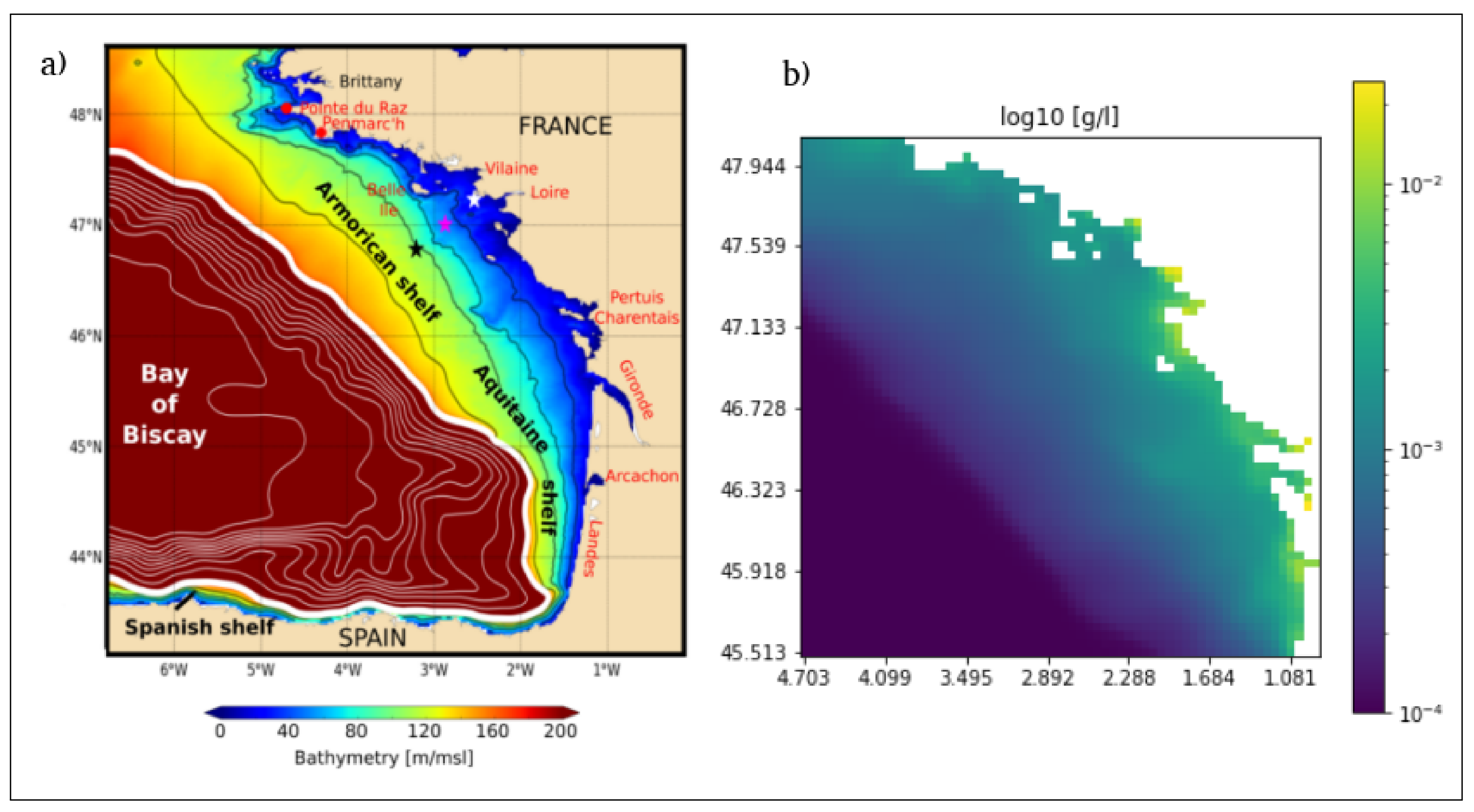
2. Case Study and Data

2.1. Data

The data used in this work are numerical simulations issued from a configuration of the coupled MARS-MUSTANG model simulating oceanic sedimentary fluxes. It includes realistic natural and anthropogenic forcings in the Bay of Biscay. These forcings comprise wind, waves, river plumes, and the general current, including tides. Anthropogenic forcings modeled are trawling from fishing vessels. In terms of particle size distribution, the model takes into account 3 sediment classes according to their mean grain size, namely mud (<63 µm), sand (from <63 µm to 2 mm), and gravel (>2 mm). The field of interest retained in this study is the sea surface total suspended sediments concentration obtained by adding the concentrations from the Sand and Mud classes (in kg·m 3 ). The gravel class had been defined in the MARS-MUSTANG model to model the bedload transport [26]. As this class does not contribute to the SSSC, it was not retained in this study.
Figure 1 illustrates the link between the bathymetry and the suspended sediment dynamics. Figure 1a displays isobaths of the Bay of Biscay, while Figure 1b displays the spatial distribution of the mean SSSC in the area of study. This shows that, as usual, higher SSSC occurs preferably in the vicinity of the coastline. Above the abyssal plain suspend sediment is nearly absent. In particular the threshold of 0.1 mg/L is well correlated with the isobath of 180 m which well represents the shelf edge. Another level of concentration, the 10 mg/L threshold, typically depicts a muddy area of the Armorican shelf also known as the “Grande Vasière”. Following, higher SSSC values at the ocean surface can be seen near estuaries of the main rivers in the area (Gironde, Loire, Vilaine, France) [27].
These MARS-MUSTANG model results have been validated with in situ and satellite data:
  • With in situ data (Reference [28], Section 4): In situ data were collected at one station of latitude 47 15.592 N and longitude 2 32.972 W, located near the coast of southern Brittany and close to the city of “Le Croisic”. There, in situ Suspended Sediment Concentration (SSC) were measured from 25 November 2007 to 31 January 2008 with an upward looking 1 MHz Acoustic Wave And Current (AWAC) Nortek profiler put, with a turbidimeter, on a bottom mooring at a depth of 23 m. The SSC has been measured in the whole water column of more than 20 m by the AWAC profiler, calibrated with the turbidimeter, itself calibrated with SSC results obtained through water samples (Reference [28], Section 2.2). Model results show good agreement with in situ data. Quantitatively, an RMSE of 10.5 mg/L between model and in situ data has been obtained for SSC (from the AWAC profiler) ranging between 10 and 80 mg/L over the whole water column.
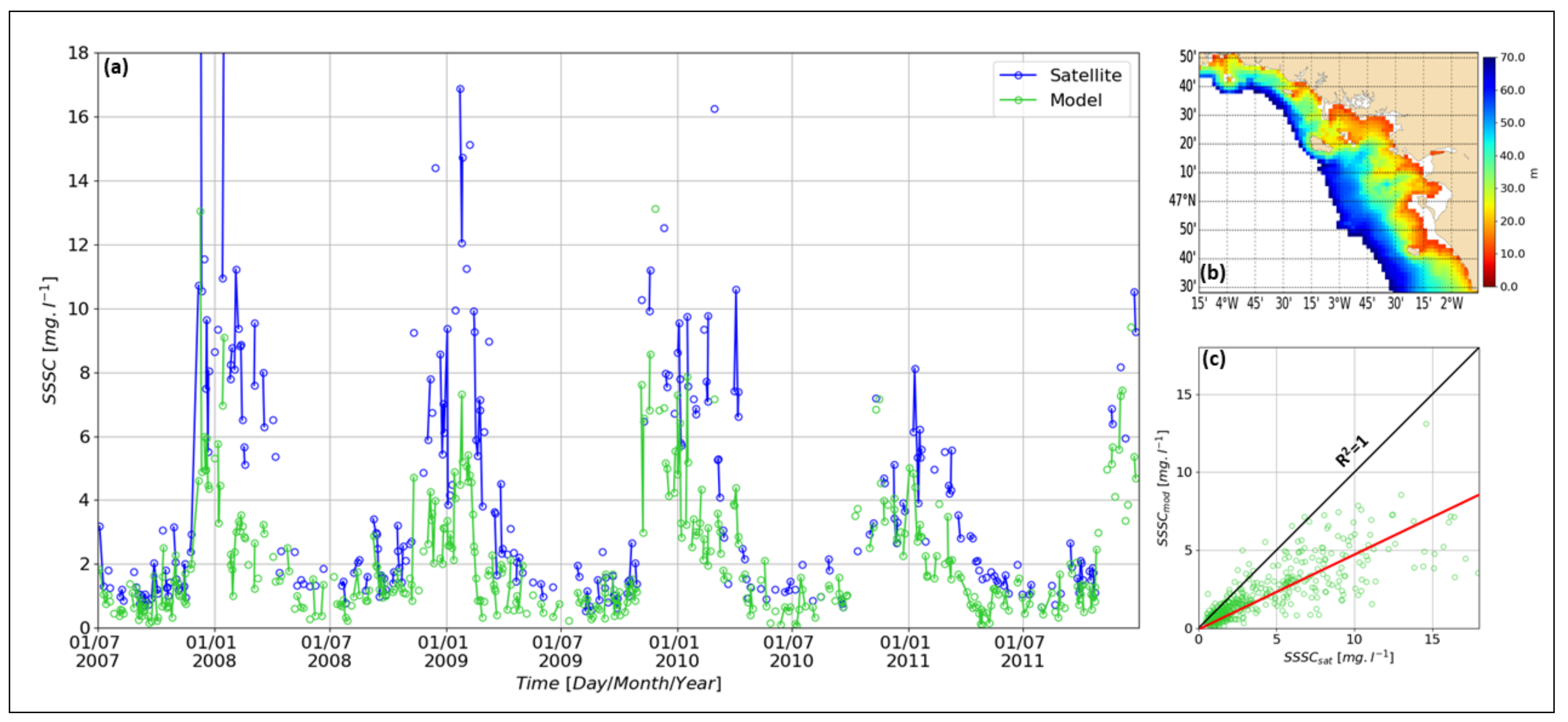
  • With satellite data; see Figure 2: The satellite data are derived from the Non Algal Particles (NAP) algorithm from [29] applied to the MERIS satellite sensor dataset available from 2007 to 2011 and daily sampled. Figure 2a,c show that MARS-MUSTANG model fit barely well with the dynamics of the turbidity observed by the satellite, but with a mean intensity in concentration that is half the mean of satellite concentrations observed through its NAP algorithm.
In this study, the overall sea surface field dataset extracted from the MARS-MUSTANG model is a time series of 1430 daily images spanning from 1 January 2007 to 8 December 2010, with a 2.5 km spatial resolution over a 64 × 64 domain. The case study region was selected to encompass proximal and distal dynamics, including fluvial sedimentary inputs.

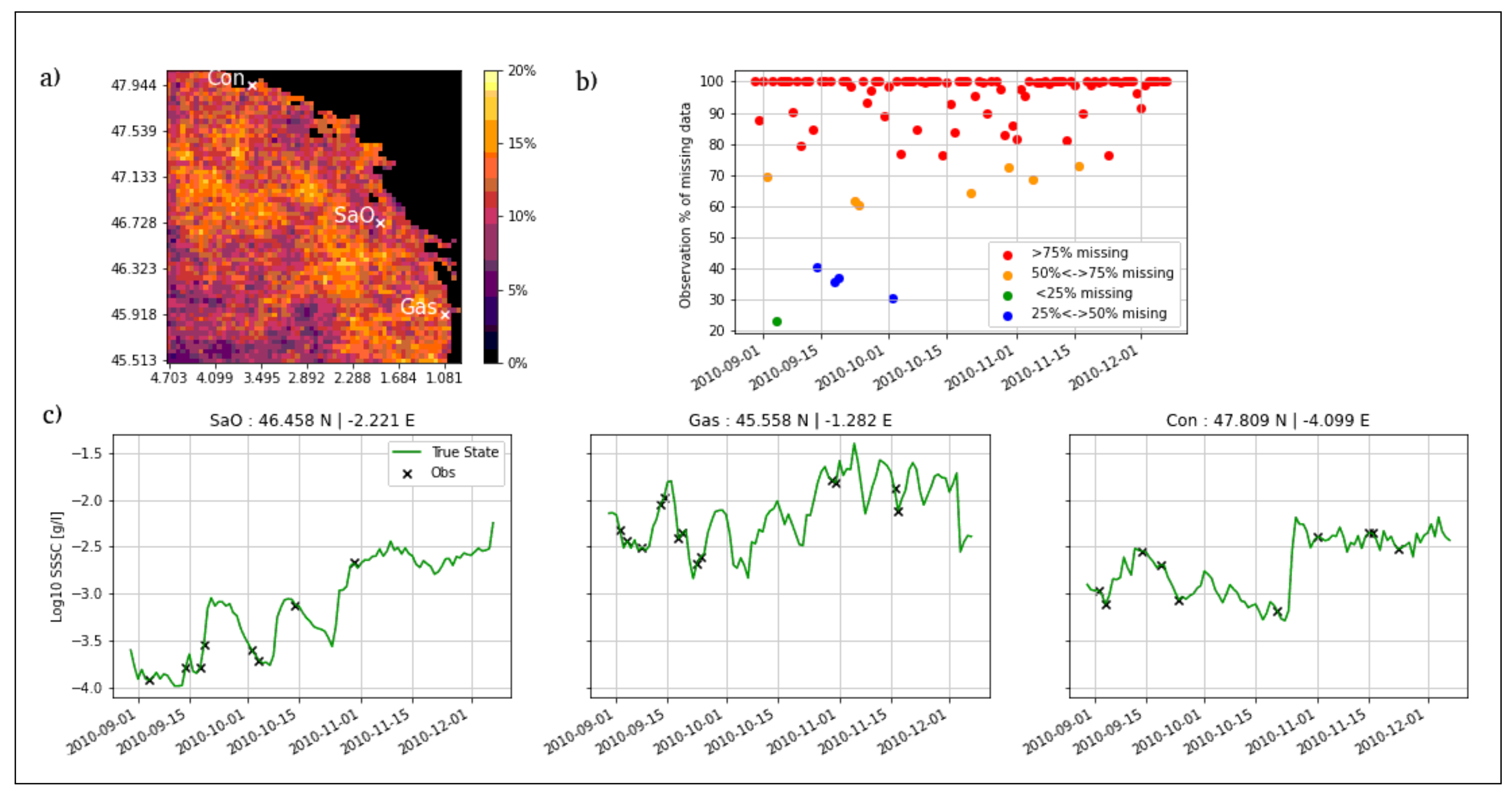
2.2. Osse and Benchmarking Framework

As illustrated in Figure 3a, ocean color satellite observations of the sea surface are scarce because sensors operate in the near-visible range and cannot observe the sea surface under cloudy conditions. This results in a high rate of missing data, having a typical mean coverage below 20% in our area of study. This missing data rate makes the interpolation task particularly challenging. It also makes complex the direct assessment of interpolation methods from satellite data. While, for moderate missing data rates (typically below 50%), one may perform benchmarking experiments from real satellite-derived datasets (e.g., Reference [21]), Observing System Simulation Experiments (OSSE) [30] provide a well-posed framework to carry out such benchmarking experiments when dealing with high missing data rates, typically above 80%. This explains why OSSE schemes are widely exploited for benchmarking experiments for the reconstruction of sea surface fields [31,32] from observation data. Especially, within an OSSE setting, the definition of the evaluation metrics do not depend on the sampling patterns of the observation data, which result in better characterization of space-time scales the interpolation methods can resolve.
The OSSE setting first relies on the availability of a reference gap-free dataset. The latter provides ground-truth states for validation purposes. Here, we use MARS-MUSTANG simulation data as the reference SSSC dataset. With a view to simulating realistic satellite-derived observation data, we generate irregularly-sampled SSC fields by applying to the reference SSSC dataset cloud masks taken from a time series of real MODIS images. We also add a Gaussian noise to the remaining SSSC values in order to simulate a satellite instrumental noise. As illustrated in Figure 3b dedicated to our case-study region, the simulated ocean color images depict missing data rates comprised between 80% and 100% of the total coverage.
As required by learning-based schemes, the OSSE dataset has been split into a training dataset and a validation dataset. The latter dataset encompasses a 100-day period spanning from 30 August 2010 to 8 December 2010. The former dataset is used for the training period that encompasses 1336 days spanning from 1 January 2007 to 30 August 2010. Since SSSC only positive values (given in mg/L) and show an asymmetric statistical distribution (broadly lognormal), all SSSC values are transformed according to a logarithm function in a preprocessing step. This can be regarded as a “pre-normalization” step prior to the application of the usual data normalization step required by learning-based techniques. During this normalization step, all SSSC values below 0.1 mg/L are set to this limit of 0.1 mg/L with the assumption that ocean color satellite sensors are able to observe below this sensitivity threshold [33].

3. Methods

This section presents the different interpolation methods we benchmark in this study. Besides Optimal Interpolation (OI), we investigate state-of-the-art data-driven techniques, namely EOF-based interpolation (DinEOF), analog data assimilation (AnDA), and neural-network interpolation schemes based on a variational formulation (4DVarNet).

3.1. Optimal Interpolation

The Optimal Interpolation (OI), also referred to as kriging [34], is a method widely applied in geophysics. Numerous operational satellite-derived products in earth science rely on OI [35]. We provide a brief description of OI and refer the reader to Reference [36] for a detailed review. OI is stated as a minimum variance estimator in linear inverse problems [37]. Knowing a set of observations y, OI computes an interpolated state x through a weighted linear mapping:
x = x b + K [ y H x b ] ,
where x b is the background information, and H a transformation matrix from the state space to the observation space. Matrix K, referred to as the Kalman gain, is given by
K = P b H T ( H B H t + R ) 1 ,
with B the prior covariance matrix of x; and R the covariance matrix of the observation noise. R is here assumed diagonal, which relates to an additive Gaussian noise. Besides the interpolated field estimate x, one may also evaluate the estimation uncertainty through posterior covariance P given by
P = P b K H P b ,
with P b as the background error covariance matrix estimated from the numerical model states.
In our experiments, we implement an OI with a Gaussian covariance model whose scale parameter was tuned through cross-validation experiments.

3.2. DINEOF

DINEOF (Data Interpolating Empirical Orthogonal Functions) is an EOF-based technique for the reconstruction of gap-free fields from irregularly-sampled observations. It exploits the spatial and/or spatio-temporal consistency of the data to deduce a solution to the missing locations [38]. DINEOF iterates a projection-reconstruction step using the EOF basis, while observed variables are kept unchanged after each iteration. We may emphasize that DINEOF may be regarded as a specific parameterization of the considered neural network schemes using an EOF decomposition as prior in the underlying variational formulation.
The implementation of DINEOF first requires selecting the number of EOF modes used for the reconstruction [22]. In our experiments, we typically consider EOF modes accounting for 99% of the total variance of the considered dataset.

3.3. AnDA

The Analog Data Assimilation (AnDA) combines an analog forecasting model to an ensemble Kalman smoother to address the data-driven space-time interpolation of spatio-temporal dynamics. A detailed description and evaluation of AnDA can be found in Reference [39]. Formally, AnDA involves a linear state-space formulation
x t = A x t 1 ( x t 1 ) + μ t ,
y t = H ( x t ) + ϵ t ,
where the linear operator A x t 1 derives from the linear approximation of the one-step-ahead mapping between analogs to state x t 1 and their successors for some referenced dataset of pairs of two successive states, referred to as a catalog. Analogs typically refer to nearest-neighbors according to some predefined similarity measure. Regarding the parameterization of the ensemble Kalman smoother, spherical covariance priors are considered for noise process μ and ϵ , and the size of the ensembles is typically set to 1000.

3.4. 4DVarNet

Deep learning schemes have rapidly become the state-of-the-art approaches for a wide range of pattern recognition and image processing applications, including in geoscience [40]. This also includes neural network approaches dedicated to interpolation issues. Recent studies [23,41] have stressed the relevance of end-to-end 4DVarNet architectures to address space-time interpolation issues with large missing data rates. Especially, these studies show that 4DVarNet architectures significantly outperform zero-filling strategies which are classically implemented for interpolation problems [42]. Applied to different case-studies, including ocean remote sensing data [23,41], they result in a significant improvement over OI, DinEOF and AnDA. To our knowledge, no prior work has investigated their application to SSC interpolation. We provide below a short introduction to 4DVarNet schemes. We refer the reader to References [42,43] for a detailed presentation.
These 4DVarNet architectures rely on the formulation of the interpolation problem as the following minimization issue
x ^ = arg min x x Φ ( x ) 2 subject to y = H · x ,
where H maps gap-free state x to the observation y, and Φ can be regarded as a projection operator. The latter states a prior on the interpolated states. For a given operator Φ , the design of a neural network architecture, which implements this algorithm, leads to an end-to-end architecture, which uses an irregularly-sampled observation as inputs, and aims at retrieving a gap-free field as outputs. This end-to-end architecture embeds an iterative solver of the above minimization problem. For instance, one may consider a fixed-point iterative algorithm similar to the one implemented by DINEOF procedure (see Section 3.2). Interestingly, this fixed-point solver is parameter-free, which results in a lighter learning-based architecture and motivates the choice considered here. Regarding operator Φ , we follow References [23,41] and explore two configurations which result in the two 4DVarNet architectures we consider in our experiments, namely:
  • AE-4DVarNet: this architecture exploits a convolutional auto-encoder (AE) architecture for operator Φ . The AE first encodes the input field x into a low-dimensional feature vector and then applies a decoder to map this feature vector to a reconstructed field Φ ( x ) . The detailed specification of the AE architecture for operator Φ is provided in Appendix A.1.
  • GE-4DVarNet: this architecture exploits a two-scale U-net-like architecture for operator Φ according to Reference [41]. Contrary to the AE-based setting, it does not involve a dimension reduction step. The resulting energy x Φ ( x ) 2 may be interpreted in terms of Markovian prior as detailed in Reference [41]. The detailed specification of the considered U-Net-like architecture Φ is reported in Appendix A.2.
The considered 4DVarNet architectures are implemented using Keras framework (Original code can be found on Github: Available online: https://github.com/CIA-Oceanix/DINAE_keras, (accessed on 5 July 2021)). The SSSC implementation is avaible on Github: Available online: https://github.com/Jvient/OSSE_BoB-4DVarNet, (accessed on 5 July 2021)). As training loss, we use a custom loss function which compute a weighted sum of Mean Absolute Errors for the SSC images and their spatial gradients. The training set-up involves Adam optimizer with a batch size of 16. We gradually increase the number of fixed-point iterations of the 4DVarNet architectures from 1 to 40 every 14 epochs.

4. Results

4.1. Metrics and Evaluation

The different interpolation methods are evaluated according to two standard metrics: the global root mean square error (RMSE) and a global reconstruction score (R-score), in terms of rate of variance of the true data captured by the interpolation. The two metrics give an general overview of the performance of a given interpolation method. Besides these global metrics, we report an evaluation for the three reference stations depicted in Figure 3a. The first location, referred to as ‘Con’, is in the northernmost zone of the case-study area close to the coastal city of Concarneau. It presents fairly high concentrations over the entire series superimposed with oscillations at a frequency of around 14–15 days, which likely relate to M2-tide forcings. The second station is located near the coastal city of Les Sables D’Olonnes (SaO) and has a steadily increasing concentration over the entire time series with oscillation at a frequency lower than Con (28 days). The last station (Gas) has been chosen near the estuary of the Gironde river. It shows a relatively flat time series, except from 4th March to 12th March, where it presents an increase in SSC, followed by a new flat series. The SSSC increase is due to a fluvial contribution from the continent observed at the end of the winter.

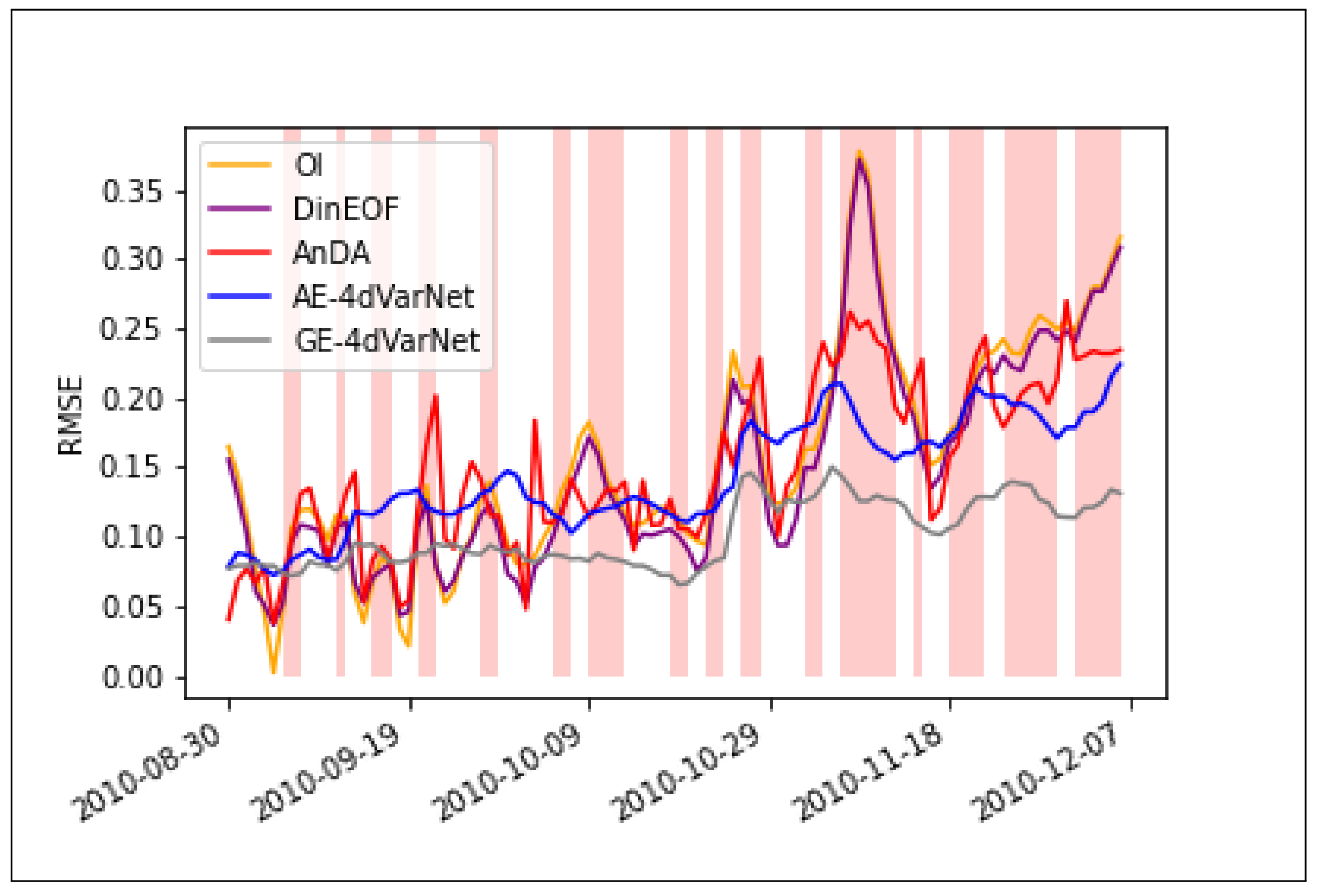
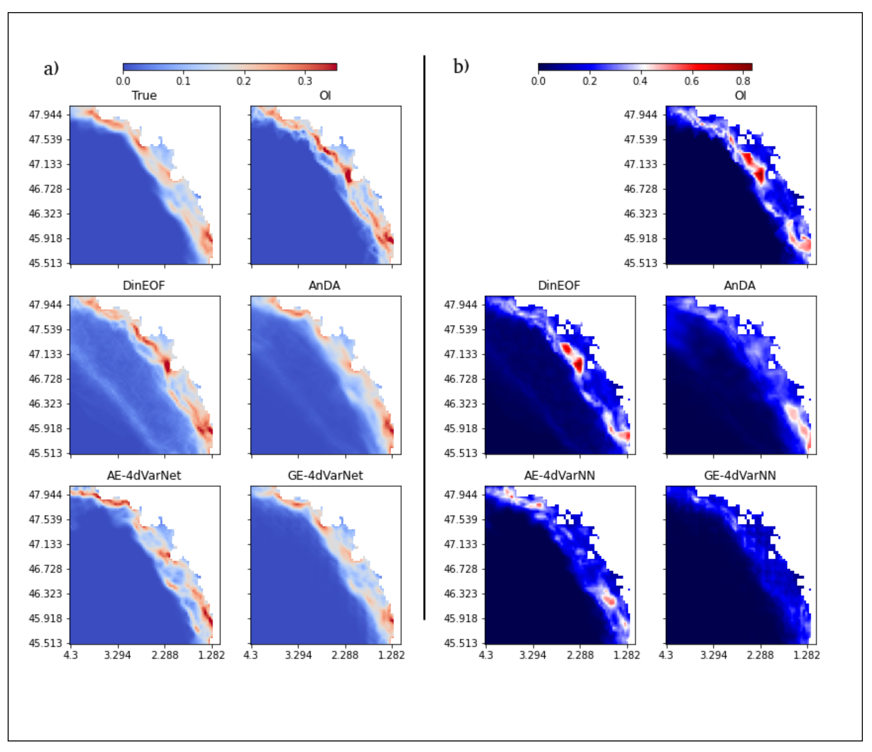
4.2. Global Performance

In Table 1, we report the global evaluation metrics of the benchmarked methods. Mean RMSE and R-score values are computed for the test dataset over the entire domain. OI performs the worst of all tested methods. However, the improvement using DINEOF and AnDA is relatively marginal, with an RMSE of 0.19 for OI versus 0.18 for DINEOF and 0.17 for AnDA over the missing data patterns. A greater improvement appears for the two neural network schemes, with a relative gain of 20% and 40% for AE-4DVarNet and GE-4DVarNet, respectively. GE-4DVarNet clearly outperforms all the other methods. Interestingly, it results in similar reconstruction performance over the observed and unobserved areas close to 96% of Explained Variance (EV), which supports a greater generalization properties of the underlying representation of the SSSC dynamics through learnt GE operator Φ . This results in an interpolation performance which is less sensitive to the rate of missing data, even for periods with high SSSC variations.
In Figure 4, interpolation scores are analyzed in function of high cloud cover periods. The time series of the daily RMSE is depicted, along with time periods where less than 5% of observations are available (red bands). The missing data rate is larger in the second part of the reconstruction period due to the gradual transition to winter with a higher cloud cover. In winter, turbidity increases with the impact of higher winds and waves, along with the sedimentary input from the continent following rainfall. The connection between the change of dynamical regime and a lack of data is a likely cause of the RMSE peaks visible on mid-October. As mentioned before, the performance of the 4DVarNet methods, and particularly GE-4DVarNet, is less affected by the cloud cover rate than other methods are. GE-4DVarNet method is also the more stable regarding smaller time-scale variations of the RMSE. The highest RMSE observed for OI and DinEOF is associated with a river plume (“Le Moros and Saint Laurent river”) containing continental inputs located in the “Baie de la Forêt” near Concarneau, that is not correctly retrieved. The underestimation of SSSC by OI is also observed for DINEOF, which may be explained by the initialization of DINEOF algorithm with the OI solution. We may point out that GE-4DVarNet also relies on the same initialization but shows a much greater ability to recover the global space-time features of the SSSC fields.
In Figure 5, we further illustrate the reconstruction of the benchmarked schemes for the norm of the gradient of the SSSC fields. This provides means to assess the ability of the different methods to retrieve the frontal structures in SSSC fields. Figure 5a further stresses, on the mean gradient field for the whole series, the better performance of GE-4DVarNet, which nicely recovers the main front structures of the true field compared with the other approaches. This is confirmed quantitatively by the map of the time-averaged RMSE map shown in Figure 5b, and global RMSE statistics are given in Table 2. More specifically, these gradient norm fields depict a clearly visible contour between coastal and open seas. This contour broadly follows the 100m isobath which borders a well-known large mud field named the “Grande Vasière”. This mud field impacts the sediment dynamics in the whole Bay of Biscay [27]. This further suggests the underlying GE representation learnt by GE-4DVarNet model for SSSC dynamics to be much more relevant than a AE-based representation in AE-4DVarNet to encode SSSC dynamics. We also interpret the lower performance retrieved by DINEOF and AnDA to be caused by a spatial smoothing effect associated with the EOF-based decomposition of the spatial variability. EOF decomposition is by construction less adapted to the retrieval of fine-scale gradient patterns.

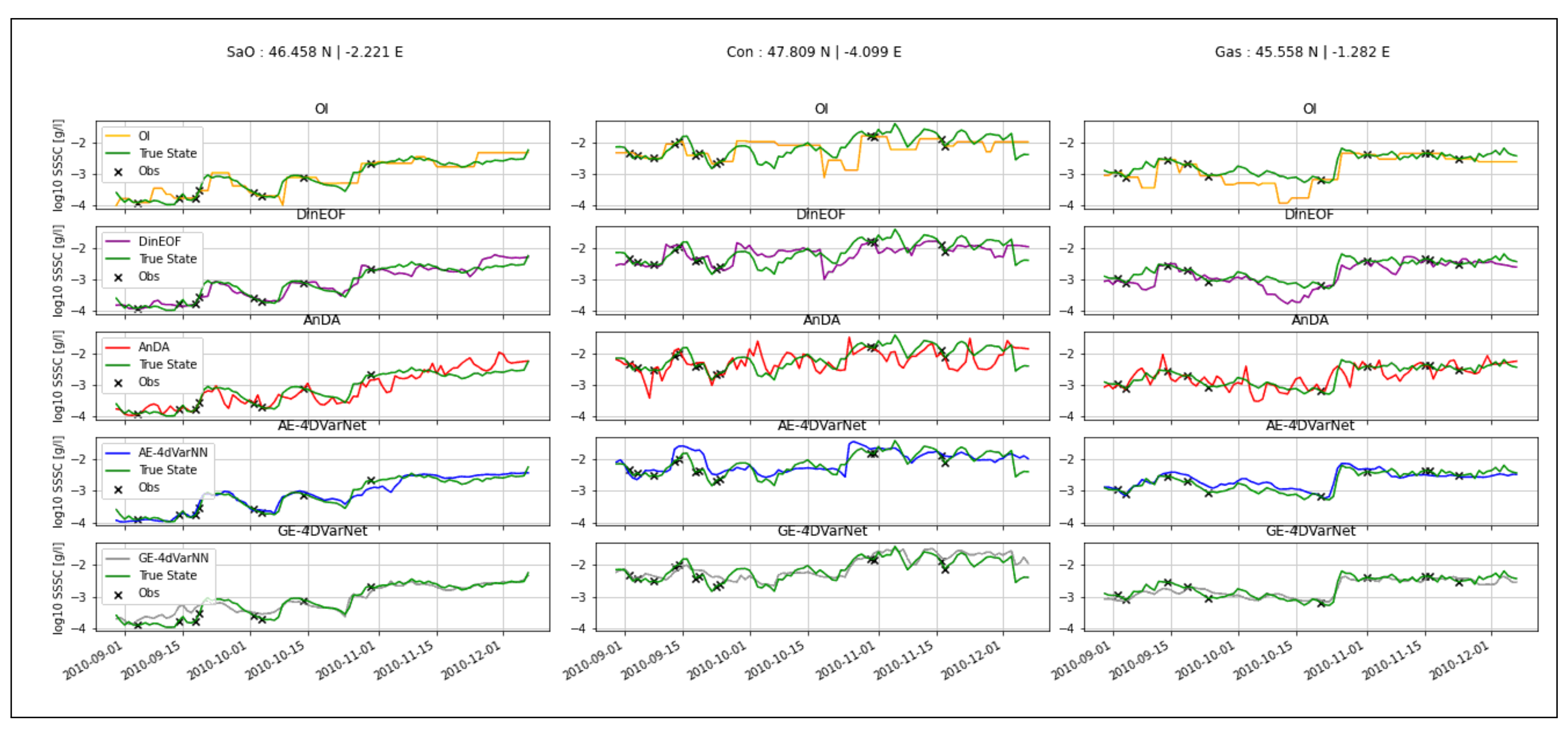
4.3. Reconstruction of Time Patterns

Besides the reconstruction of spatial patterns, we also investigate whether the interpolated fields provide a relevant characterization of the variations of SSSC with time. In Figure 6, we compare the time series of the true SSSC to the interpolated time series for the three selected stations, namely SaO, Gas, Con as defined in Figure 3. GE-4DVarNet reaches the greatest correlation with respect to the groundtruth. This is confirmed by the visual inspection of the different series. For instance, the GE-4DVarNet reconstruction fits very well the true series at ‘Con’ station for abrupt change occurring at day 20 November 2021. By contrast, the other schemes seem to produce some fine-scale artifacts, which may relate to some erroneous reconstruction of spatial gradients as discussed above. Interestingly, GE-4DVarNet also recovers the 14-day oscillation related to the M2 tide process even with a high missing data rate. This may relate to spectral features captured by the GE representation of sediment dynamics learnt by GE-4dVarNet.

5. Discussion

The goal of this study has been to assess the performance of interpolation methods for the retrieval of gap-free series of SSC fields from irrgegularly-sampled satellite-derived measurements. Given the typical cloud cover for mid-latitude areas (about 80% of missing data in our case-study), we implemented an OSSE framework to evaluate the potential of data-driven approaches, which have recently emerged as relevant alternatives to model-driven assimilation products [9,18,21] and operational OI schemes [44,45]. Interestingly, our study stresses that the selection of the interpolation methods may strongly affect the ability to retrieve some features of SSSC dynamics. For instance, the best scheme (GE-4DVarNet) results in a relative gain with respect to OI in terms of RMSE greater than 40%. We believe that this OSSE could provide a relevant benchmark for future development of SSSC interpolation methods. We make available online our dataset and the associated evaluation framework (Data and code available at: https://github.com/Jvient/OSSE_BoB-4DVarNet, (accessed on 5 July 2021)).
Among the three classes of data-driven interpolation schemes, the neural network approaches were the ones leading to a significant improvement with respect to the OI baseline. Both DinEOF and AnDA rely on an EOF decomposition for the spatial variability of SSS dynamics. Their interpolation results suffer from similar limitation with a relatively poor ability to retrieve frontal structures. As the missing data rates are greater than 80%, the EOF decomposition may not be appropriate to appropriately capture relevant space-time scales of SSSC dynamics from the observed data. By contrast, neural network approaches learn the representation of the gap-free fields through operator Φ so that the interpolation performance is optimized. This is expected to result in a representation of SSSC dynamics which is more adapted to the interpolation problem.
Overall, our study clearly advocates for the design and development of neural network schemes for the interpolation of SSSC fields. For GE-4DvarNet scheme, we reported a mean relative gain with respect to OI in terms of RMSE is of 41% for the log10(SSSC) values and of 35% for their gradient norm. Besides, these global performance metrics, we also showed that the resulting interpolations may capture relevant spatial patterns (e.g., the impact of a well-known mud field zone in the case-study area) and time scales (e.g., M2-tide forcings exhibited at station Con), which were not retrieved using the other approaches. These results are in line with other studies dedicated to other sea surface geophysical parameters, namely sea surface temperature (SST) [21,41] and sea surface height (SSH) [41]. These studies also highlighted the greater ability of neural network approaches based on a variational formulation to learn relevant interpolation algorithms when dealing with large missing data rates: typically from 50% to 75% for SST and below 10% for SSH. Intesretingly, 4dVarNet schemes also relate to variational data assimilation models. This may be of interest to exploit some model-driven priors onto the considered geophysical dynamics when available [41].
These results show that NN-based methods outperform the interpolation rate of this OSSE. The common main reasons for this is that these methods exploit much more past observations for the present reconstruction. Indeed, when applying an OI in a multi-map context with a total absence of data, it is necessary to extend the spatial influence of the Gaussian kernel and obtain a covariance matrix that can provide results [46]. This extension of the neighborhood search to observations implies a more important smoothing of the map during the completed interpolation. Concerning the EOF-based methods (DinEOF and AnDA) the main source of errors comes from the noise allocated to the simulated observations. Indeed, the latter results from DinEOF and AnDA display high frequency spatial patterns that can be caused by a bad decomposition of the signal. In addition, these bad patterns are assimilated in the same way as real high frequency events. Thus, when reconstructing the images, and, despite the fact that 95% of the explained variance has been selected, the result leads to a worse reconstruction, especially in the higher dynamic range [22].
All the considered data-driven approaches rely on the availability of a reference gap-free dataset during the training phase. This is particularly important for neural network approaches. The applicability of the trained models to real satellite-derived datasets particularly depends on ability of numerical simulations to represent the targeted SSSC dynamics. Numerical simulations cannot in general address all the processes in play in real observation data. For instance, the MARS-MUSTANG model used here does not simulate the fate of detritic particles that appear in real satellite observations of SSSC fields. We may also point out that the additive Gaussian instrumental noise is likely not an accurate representation of real satellite sensor errors. We then regard the reported interpolation performance as a lower-bound of the performance that could be retrieved for real observation datasets. Future work shall further explore the application and adaption of the proposed schemes to real satellite datasets. Regarding 4DVarNet approaches, we can envision different learning strategies. We may first explore a full training from scratch of the proposed scheme. In our study, we used a 3-year gap-free datasets for training. For real satellite data, we may exploit a 20-year time series. With a mean cloud coverage of 85% over our area of study (cf. Figure 3), the number of data available for the learning process is roughly equivalent to a 3-year gap-free dataset. This makes the training of 4DvarNet models from real observation dataset a realistic option to be explored. Transfer learning strategies [47,48], which would exploit pre-trained models using the proposed OSSE before adapting them to real observation datasets, also appear as a promising direction. These strategies shall require smaller real datasets compared with training models from scratch.
The application to real observation datasets could also benefit from several extensions of the considered 4DVarNet schemes. First of all, such schemes could easily embed covariates to further constrain the interpolation process, including among others the bathymetry or metocean covariates. We believe that these schemes may also open new avenues for short-term forecasting issues from gappy satellite observation data [43], as forecasting issues may be regarded as an interpolation problem in which the future is masked. Future work shall also investigate the estimation of some uncertainty of the interpolation. Different studies [49,50] provide methodological backgrounds to embed such an uncertainty component in 4DVarNet schemes.

6. Conclusions

In this study, we have addressed the data-driven interpolation of satellite-derived SSSC fields. An OSSE setting in Bay of Biscay has shown that data-driven schemes, especially neural-network architectures backed by a variational formulation for space-time interpolation, can significantly improve the reconstruction of SSSC dynamics compared with an OI, which is classically used in deriving operational products. Our experiments support a greater performance of GE-4DVarNet scheme both to recover spatial and temporal patterns with a relative gain up to 40% in terms of RMSE w.r.t. the groundtruth. These results are in line with recent experiments using other satellite-derived sea surface parameters, such as sea surface height [23] and sea surface temperature [20,21].
With possible applications not only to interpolation but also to forecasting or model identification, the 4DVarNet methods may open new research avenues for the modeling, reconstruction, and forecasting of sediment dynamics from partial satellite-derived observations with direct operational impacts on the short-term.

7. Materials

All code and samples are available here: Available online: https://github.com/Jvient/OSSE_BoB-4DVarNet (accessed on 5 July 2021).

Author Contributions

Conceptualization, R.F., C.D. and F.J.; methodology, R.F.; software, J.-M.V.; validation, J.-M.V., C.D. and L.L.; formal analysis, C.D.; resources, B.M.; data curation, B.M. and L.L.; writing—original draft preparation, J.-M.V.; writing—review and editing, F.J., J.-M.V. and R.F.; visualization, L.L.; supervision, C.D. All authors have read and agreed to the published version of the manuscript.

Funding

This research received no external funding.

Institutional Review Board Statement

Not applicable.

Informed Consent Statement

Not applicable.

Data Availability Statement

Data are available in the code package available in Github link: https://github.com/Jvient/OSSE_BoB-4DVarNet (accessed on 5 July 2021).

Acknowledgments

This research was funded by the AID (French Agency of Defense Innovation through a PhD scholarship and the city of Brest (BMO). It was also supported by ANR Project OceaniX. It benefited from HPC and GPU resources from Azure (Microsoft EU Ocean awards).

Conflicts of Interest

The authors declare no conflict of interest.

Appendix A

Appendix A.1. Architecture of the Autoencoder Operator ϕ (AE-NN)

A convolutional AutoEncoder formulation based on encoding (E) and decoding (D) operator. First, E reduces the dimension of the domain to a lower dimensional space. Its architecture is based on 5 Conv2D layers. We first consider a convolutional auto-encoder as proposed in References [20,21] as follows. The encoder, which maps the input data to a low-dimensional space, involves the following five-layer CNN:
  • Conv2D (Relu activation, 30 filters, 3 × 3 kernels, average pooling layer);
  • Conv2D (Relu activation, 60 filters, 3 × 3 kernels, average pooling layer);
  • Conv2D (Relu activation, 120 filters, 3 × 3 kernels, average pooling layer);
  • Conv2D (Relu activation, 240 filters, 6 × 6 kernels, average pooling layer);
  • Conv2D (Linear activation, 30 filters, 3 × 3 kernels).
D project the low dimensional encoding representation into the original space. Its architecture is composed of Conv2Dtranspose layer and Conv2D layer. The resulting encoding space if a 2 × 2 × 30 space. Regarding the decoder, we consider a classic convolutional architecture using Conv2Dtranspose upsampling layers:
  • Conv2DTranspose (Relu activation, 256 filters, 8 × 8 kernels);
  • Conv2DTranspose (Relu activation, 128 filters, 3 × 3 kernels);
  • Conv2DTranspose (Relu activation, 64 filters, 3 × 3 kernels);
  • Conv2DTranspose (Relu activation, 20 filters, 3 × 3 kernels);
  • Conv2D (Relu activation, 40 filters, 3 × 3 kernels, average pooling layer);
  • Conv2D (Linear activation, 64 filters, 3 × 3 kernels).
Overall, this ConvAE model involves 500 k parameters.

Appendix A.2. Architecture of the Gibbs-Energy Operator ϕ (GE-NN)

The NN is based on two NN energy. A parameterization of operator Φ which relates to Markov random fields [20,50] has also been explored. It does not rely on dimension reduction hypothesis as the previous one. A good state-space reconstruction refers to a low-energy state, where at any space position s and time step t, Φ ( x ) ( s , t ) only involves state x in a space-time neighborhood of ( s , t ) . The following architecture is used:
  • AveragePolinglayer (4 × 4);
  • Conv2D (Relu activation, 40 filters, 3 × 3 kernels) with a null-weight constraint for the center of the convolution window;
  • Conv2D (Relu activation, 40 filters, 1 × 1 kernels);
  • a residual network [51] with the following residual block: Conv2D (Relu activation, 240 filters, 200 × 200 × (5 × 40) kernels, average pooling layer);
    Conv2D ( Relu activation, 40 filters, 1 × 1 kernel);
  • Upsampling to the original input shape is processed by a Conv2DTranspose (Linear activation, 4 × 4 kernels).
This GE-4DVarNet model involves 80 k parameters, which is much more compact than the AE-4DVarNet architecture.

References

  1. Owens, P.N. Soil erosion and sediment dynamics in the Anthropocene: A review of human impacts during a period of rapid global environmental change. J. Soils Sediments 2020, 20, 4115–4143. [Google Scholar] [CrossRef]
  2. Irabien, M.J.; Cearreta, A.; Gómez-Arozamena, J.; Gardoki, J.; Martín-Consuegra, A.F. Recent coastal anthropogenic impact recorded in the Basque mud patch (southern Bay of Biscay shelf). Quat. Int. 2020, 566–567, 357–367. [Google Scholar] [CrossRef]
  3. Brand, E.; Chen, M.; Montreuil, A.L. Optimizing measurements of sediment transport in the intertidal zone. Earth-Sci. Rev. 2020, 200. [Google Scholar] [CrossRef]
  4. Vercruysse, K.; Grabowski, R.C.; Rickson, R.J. Suspended sediment transport dynamics in rivers: Multi-scale drivers of temporal variation. Earth-Sci. Rev. 2017, 166, 38–52. [Google Scholar] [CrossRef] [Green Version]
  5. Haalboom, S.; de Stigter, H.; Duineveld, G.; van Haren, H.; Reichart, G.J.; Mienis, F. Suspended particulate matter in a submarine canyon (Whittard Canyon, Bay of Biscay, NE Atlantic Ocean): Assessment of commonly used instruments to record turbidity. Mar. Geol. 2021, 434, 10639. [Google Scholar] [CrossRef]
  6. Le Hir, P.; Monbet, Y.; Orvain, F. Sediment erodability in sediment transport modelling: Can we account for biota effects? Cont. Shelf Res. 2007, 27, 1116–1142. [Google Scholar] [CrossRef]
  7. Wang, Y.P.; Voulgaris, G.; Li, Y.; Yang, Y.; Gao, J.; Chen, J.; Gao, S. Sediment resuspension, flocculation, and settling in a macrotidal estuary. J. Geophys. Res. Ocean. 2013. [Google Scholar] [CrossRef]
  8. Allard, R.; Barron, C.; Blain, C.A.; Hogan, P.; Keen, T.; Smedstad, L.; Wallcraft, A.; Berger, C.; Howington, S.; Smith, J.; et al. High Fidelity Simulations of Littoral Environments; Office of Naval Research, Stennis Space Center: Hancock County, MS, USA, 2003; p. 16. [Google Scholar]
  9. Renosh, P.R.; Jourdin, F.; Charantonis, A.A.; Yala, K.; Rivier, A.; Badran, F.; Thiria, S.; Guillou, N.; Leckler, F.; Gohin, F.; et al. Construction of multi-year time-series profiles of suspended particulate inorganic matter concentrations using machine learning approach. Remote Sens. 2017, 9, 1320. [Google Scholar] [CrossRef] [Green Version]
  10. Moore, A.M.; Martin, M.J.; Akella, S.; Arango, H.G.; Balmaseda, M.; Bertino, L.; Ciavatta, S.; Cornuelle, B.; Cummings, J.; Frolov, S.; et al. Synthesis of ocean observations using data assimilation for operational, real-time and reanalysis systems: A more complete picture of the state of the ocean. Front. Mar. Sci. 2019, 6, 1–6. [Google Scholar] [CrossRef] [Green Version]
  11. Nazeer, M.; Bilal, M.; Alsahli, M.; Shahzad, M.; Waqas, A. Evaluation of Empirical and Machine Learning Algorithms for Estimation of Coastal Water Quality Parameters. ISPRS Int. J. Geo-Inf. 2017, 6, 360. [Google Scholar] [CrossRef] [Green Version]
  12. Jin, D.; Lee, E.; Kwon, K.; Kim, T. A Deep Learning Model Using Satellite Ocean Color and Hydrodynamic Model to Estimate Chlorophyll- a Concentration. Remote Sens. 2021, 13, 2003. [Google Scholar] [CrossRef]
  13. Sanchez-Arcilla, A.; Staneva, J.; Cavaleri, L.; Badger, M.; Bidlot, J.; Sorensen, J.T.; Hansen, L.B.; Martin, A.; Saulter, A.; Espino, M.; et al. CMEMS-Based Coastal Analyses: Conditioning, Coupling and Limits for Applications. Front. Mar. Sci. 2021, 8. [Google Scholar] [CrossRef]
  14. He, X.; Bai, Y.; Pan, D.; Huang, N.; Dong, X.; Chen, J.; Chen, C.T.A.; Cui, Q. Using Geostationary Satellite Ocean Color Data to Map the Diurnal Dynamics of Suspended Particulate Matter in Coastal Waters. Remote Sens. Environ. 2013, 133, 225–239. [Google Scholar] [CrossRef]
  15. Ping, B.; Su, F.; Meng, Y. An improved DINEOF algorithm for filling missing values in spatio-temporal sea surface temperature data. PLoS ONE 2016, 11, 1–12. [Google Scholar] [CrossRef] [Green Version]
  16. Tandeo, P.; Ailliot, P.; Ruiz, J.; Hannart, A.; Chapron, B.; Cuzol, A.; Monbet, V.; Easton, R.; Fablet, R. Combining Analog Method and Ensemble Data Assimilation: Application to the Lorenz-63 Chaotic System. Mach. Learn. Data Min. Approaches Clim. Sci. 2015, 3–12. [Google Scholar] [CrossRef] [Green Version]
  17. Kim, Y.H.; Im, J.; Ha, H.K.; Choi, J.K.; Ha, S. Machine learning approaches to coastal water quality monitoring using GOCI satellite data. GIScience Remote Sens. 2014. [Google Scholar] [CrossRef]
  18. Ouala, S.; Herzet, C.; Fablet, R. Sea surface temperature prediction and reconstruction using patch-level neural network representations. arXiv 2018, arXiv:1806.00144. [Google Scholar]
  19. Liu, X.; Wang, M. Super-Resolution of VIIRS-Measured Ocean Color Products Using Deep Convolutional Neural Network. IEEE Trans. Geosci. Remote Sens. 2021, 59, 114–127. [Google Scholar] [CrossRef]
  20. Fablet, R.; Drumetz, L.; Rousseau, F. End-to-end learning of energy-based representations for irregularly-sampled signals and images. arXiv 2019, arXiv:1910.00556. [Google Scholar]
  21. Barth, A.; Alvera-Azcárate, A.; Licer, M.; Beckers, J.M. DINCAE 1.0: A convolutional neural network with error estimates to reconstruct sea surface temperature satellite observations. Geosci. Model Dev. 2020, 13, 1609–1622. [Google Scholar] [CrossRef] [Green Version]
  22. Alvera-Azcárate, A.; Vanhellemont, Q.; Ruddick, K.; Barth, A.; Beckers, J.M. Analysis of high frequency geostationary ocean colour data using DINEOF. Estuar. Coast. Shelf Sci. 2015. [Google Scholar] [CrossRef] [Green Version]
  23. Beauchamp, M.; Fablet, R.; Ubelmann, C.; Ballarotta, M.; Chapron, B. Intercomparison of data-driven and learning-based interpolations of along-track nadir and wide-swath swot altimetry observations. Remote Sens. 2020, 12, 3806. [Google Scholar] [CrossRef]
  24. Tew-Kai, E.; Quilfen, V.; Cachera, M.; Boutet, M. Dynamic coastal-shelf seascapes to support marine policies using operational coastal oceanography: The french example. J. Mar. Sci. Eng. 2020, 8, 585. [Google Scholar] [CrossRef]
  25. Doray, M.; Petitgas, P.; Romagnan, J.B.; Huret, M.; Duhamel, E.; Dupuy, C.; Spitz, J.; Authier, M.; Sanchez, F.; Berger, L.; et al. The PELGAS survey: Ship-based integrated monitoring of the Bay of Biscay pelagic ecosystem. Prog. Oceanogr. 2018, 166, 15–29. [Google Scholar] [CrossRef] [Green Version]
  26. Mengual, B.; Le Hir, P.; Cayocca, F.; Garlan, T. Bottom trawling contribution to the spatio-temporal variability of sediment fluxes on the continental shelf of the Bay of Biscay (France). Mar. Geol. 2019, 414, 77–91. [Google Scholar] [CrossRef]
  27. Mengual, B. Spatio-Temporal Variability of Sediment Fluxes in the Bay of Biscay: Relative Contributions of Climate Forcings and Trawling Activities; Technical Report; Earth Sciences; Universite de Bretagne Occidentale-Brest: Brest, France, 2016. [Google Scholar]
  28. Mengual, B.; Hir, P.L.; Cayocca, F.; Garlan, T. Modelling fine sediment dynamics: Towards a common erosion law for fine sand, mud and mixtures. Water 2017, 9, 564. [Google Scholar] [CrossRef] [Green Version]
  29. Gohin, F. Annual cycles of chlorophyll-a, non-algal suspended particulate matter, and turbidity observed from space and in-situ in coastal waters. Ocean. Sci. 2011, 7, 705–732. [Google Scholar] [CrossRef] [Green Version]
  30. Hoffman, R.N.; Atlas, R. Future observing system simulation experiments. Bull. Am. Meteorol. Soc. 2016, 97, 1601–1616. [Google Scholar] [CrossRef]
  31. Leidner, S.M.; Annane, B.; McNoldy, B.; Hoffman, R.; Atlas, R. Variational analysis of simulated ocean surface winds from the cyclone Global Navigation Satellite System (CYGNSS) and evaluation using a regional OSSE. J. Atmos. Ocean. Technol. 2018, 35, 1571–1584. [Google Scholar] [CrossRef]
  32. Halliwell, G.R.; Mehari, M.F.; Le Hénaff, M.; Kourafalou, V.H.; Androulidakis, I.S.; Kang, H.S.; Atlas, R. North Atlantic Ocean OSSE system: Evaluation of operational ocean observing system components and supplemental seasonal observations for potentially improving tropical cyclone prediction in coupled systems. J. Oper. Oceanogr. 2017, 10, 154–175. [Google Scholar] [CrossRef]
  33. Morel, A.; Bélanger, S. Improved detection of turbid waters from ocean color sensors information. Remote Sens. Environ. 2006, 102, 237–249. [Google Scholar] [CrossRef]
  34. Cressie, N.A.C.; Wikle, C.K. Statistics for Spatio-Temporal Data; Wiley John Wiley and Sons: Hoboken, NJ, USA, 2011; p. 588. [Google Scholar]
  35. Høyer, J.L.; She, J. Optimal interpolation of sea surface temperature for the North Sea and Baltic Sea. J. Mar. Syst. 2007. [Google Scholar] [CrossRef]
  36. Daley, R. Atmospheric data Assimilation. J. Meterological Soc. Jpn. 1997, 75, 319–329. [Google Scholar] [CrossRef] [Green Version]
  37. Oliver, M.A.; Webster, R. Kriging: A method of interpolation for geographical information systems. Int. J. Geogr. Inf. Syst. 2007, 4, 313–332. [Google Scholar] [CrossRef]
  38. Beckers, J.M.; Rixen, M.; Beckers, J.M.; Rixen, M. EOF Calculations and Data Filling from Incomplete Oceanographic Datasets*. J. Atmos. Ocean. Technol. 2003, 20, 1839–1856. [Google Scholar] [CrossRef]
  39. Lguensat, R.; Tandeo, P.; Ailliot, P.; Pulido, M.; Fablet, R. The Analog Data Assimilation. Mon. Weather. Rev. 2017. [Google Scholar] [CrossRef] [Green Version]
  40. Zhang, L.; Zhang, L.; Du, B. Deep learning for remote sensing data: A technical tutorial on the state of the art. IEEE Geosci. Remote. Sens. Mag. 2016, 4, 22–40. [Google Scholar] [CrossRef]
  41. Fablet, R.; Amar, M.M.; Febvre, Q.; Beauchamp, M.; Chapron, B. End-To-End Physics-Informed Representation Learning for Satellite Ocean Remote Sensing Data: Applications To Satellite Altimetry and Sea Surface Currents. ISPRS Ann. Photogramm. Remote Sens. Spat. Inf. Sci. 2021, 3, 295–302. [Google Scholar] [CrossRef]
  42. Fablet, R.; Chapron, B.; Drumetz, L.; Memin, E.; Pannekoucke, O.; Rousseau, F. Learning variational data assimilation models and solvers. arXiv 2020, arXiv:2007.12941. [Google Scholar]
  43. Fablet, R.; Beauchamp, M.; Drumetz, L.; Rousseau, F. Joint Interpolation and Representation Learning for Irregularly Sampled. Front. Appl. Math. Stat. 2021, 7, 1–13. [Google Scholar] [CrossRef]
  44. Tomas-Burguera, M.; Beguería, S.; Vicente-Serrano, S.; Maneta, M. Optimal Interpolation scheme to generate reference crop evapotranspiration. J. Hydrol. 2018, 560, 202–219. [Google Scholar] [CrossRef]
  45. Lorenzo, A.T.; Morzfeld, M.; Holmgren, W.F.; Cronin, A.D. Optimal interpolation of satellite and ground data for irradiance nowcasting at city scales. Sol. Energy 2017, 144, 466–474. [Google Scholar] [CrossRef] [Green Version]
  46. Zhen, Y.; Tandeo, P.; Leroux, S.; Metref, S.; Penduff, T.; Le Sommer, J. An adaptive optimal interpolation based on analog forecasting: Application to ssh in the gulf of Mexico. J. Atmos. Ocean. Technol. 2020, 37, 1697–1711. [Google Scholar] [CrossRef]
  47. Weiss, K.; Khoshgoftaar, T.M.; Wang, D.D. A Survey of Transfer Learning; Springer International Publishing: London, UK, 2016; Volume 3. [Google Scholar] [CrossRef] [Green Version]
  48. Orenstein, E.C.; Beijbom, O. Transfer learning and deep feature extraction for planktonic image data sets. In Proceedings of the 2017 IEEE Winter Conference on Applications of Computer Vision, WACV 2017, Santa Rosa, CA, USA, 24–31 March 2017; pp. 1082–1088. [Google Scholar] [CrossRef]
  49. Sidén, P.; Lindsten, F. Deep Gaussian markov random fields. In Proceedings of the 37th International Conference on Machine Learning, ICML 2020, Virtual, 13–18 July 2020; PartF16814. pp. 8875–8885. [Google Scholar]
  50. Barth, A.; Azcárate, A.A.; Joassin, P.; Beckers, J.M.; Troupin, C. Statistical Analysis of Biological data and Times-Series Introduction to Optimal Interpolation and Variational Analysis Theory of optimal interpolation and variational analysis Contents. In Statistical Analysis of Biological Data and Times-Series; GeoHydrodynamics and Environment Research; University of Liege: Liege, Belgium, 2008; Chapter 1. [Google Scholar]
  51. Li, Y.; Allen-Zhu, Z. What can resnet learn efficiently, going beyond kernels? arXiv 2019, arXiv:1905.10337. [Google Scholar]
Figure 1. (a) Bathymetry of the Bay of Biscay. Black lines represent isobaths 40, 70, 100, and 130 m. The thick white line (corresponding to the 180 m isobath) approximately delimits the shelf edge. (b) Mean spatial distribution of the log10 SSSC (g/L) from the MARS-MUSTANG hydrosedimentary model.
Remotesensing 13 03537 g001
Figure 2. Comparison of daily satellite SSSC [29] (SSSC s a t ) with model results (SSSC m o d ). (a) SSSC time series in mg/L (constrained by the daily frequency of satellite observations) along the 2007–2011 period, averaged over the 10–70 m bathymetric range of the area of interest plotted in (b). Time series on (a) are masked when the cloud cover is higher than 90% over the area of interest. (c) Correlations between modeled and observed SSSC, where continuous and red line refer to model underestimations (with respect to observations) by a factor of 2.
Remotesensing 13 03537 g002
Figure 3. Illustration of key features of the considered OSSE dataset: (a) Map of pixel-wise available data rates for the simulated SSSC dataset, with, depicted in white, the location of the three reference stations named ‘SaO’, ‘Gas’, and ‘Con’. (b) Time series of the missing data rate for the simulated SSSC dataset. (c) Time series of the reference SSSC dataset (in green) for the three reference stations, and where black crosses are drawn when the pixel corresponding to each station is observed by the satellite.
Remotesensing 13 03537 g003
Figure 4. Daily reconstruction RMSE for OI, DinEOF, AndA, AE-4DVarNet, and GE-4DVarNet. Red bars indicate time periods having a daily missing data rate above 95%.
Remotesensing 13 03537 g004
Figure 5. Reconstruction of SSSC gradient fields: (a) reconstruction obtained by OI, AnDA, DINEOF, AE-4DVarNet, and GE-4DVarNet on average for the whole 100-day validation period. (b) map of the mean reconstruction error for the 100-day validation period for OI, DinEOF, AnDA, AEP-4DVarNet, and GE-4DVarNet.
Remotesensing 13 03537 g005
Figure 6. Time series of the SSSC reconstruction for OI, DinEOF, AnDA, AE-4DVarNet, and GE-4DVarNet. Green series refer to true state, mark to the observational term inputs.
Remotesensing 13 03537 g006
Table 1. RMSE and R-score computed for all methods over the SSSC validation period: these scores are computed globally (All) and over the observed data (Observed) and the missing data (Unobserved) patterns.
ErrorUnitData DomainOIDinEOFAnDAAE-4DVarNetGE-4DVarNet
RMSE log 10 [g/L]All0.1760.1670.1620.1420.104
R-score%All90.491.391.993.796.6
RMSE log 10 [g/L]Observed0.0560.0380.0490.0950.094
R-score%Observed98.599.499.392.896.4
RMSE log 10 [g/L]Unobserved0.1870.1770.1710.1510.106
R-score%Unobserved89.590.591.293.296.6
Table 2. Mean RMSE and R-score for the norm of the SSSC gradients computed for all methods over the 100-day validation period.
GlobalUnitOIDinEOFAnDAAE-4DVarNetGE-4DVarNet
RMSE log 10 [g/L]/m0.1100.0930.0790.0840.073
R-score%16.040.657.151.163.7
Publisher’s Note: MDPI stays neutral with regard to jurisdictional claims in published maps and institutional affiliations.

