Efficient and Flexible Aggregation and Distribution of MODIS Atmospheric Products Based on Climate Analytics as a Service Framework

Abstract

MODIS (Moderate Resolution Imaging Spectroradiometer) is a key instrument onboard NASA’s Terra (launched in 1999) and Aqua (launched in 2002) satellite missions as part of the more extensive Earth Observation System (EOS). By measuring the reflection and emission by the Earth-Atmosphere system in 36 spectral bands from the visible to thermal infrared with near-daily global coverage and high-spatial-resolution (250 m ~ 1 km at nadir), MODIS is playing a vital role in developing validated, global, interactive Earth system models. MODIS products are processed into three levels, i.e., Level-1 (L1), Level-2 (L2) and Level-3 (L3). To shift the current static and “one-size-fits-all” data provision method of MODIS products, in this paper, we propose a service-oriented flexible and efficient MODIS aggregation framework. Using this framework, users only need to get aggregated MODIS L3 data based on their unique requirements and the aggregation can run in parallel to achieve a speedup. The experiments show that our aggregation results are almost identical to the current MODIS L3 products and our parallel execution with 8 computing nodes can work 88.63 times faster than a serial code execution on a single node.

1. Introduction

In the past few decades, the emergence of terabyte remote sensing data offers an excellent chance for Earth Science study. As a remote sensing instrument, the MODIS (Moderate Resolution Imaging Spectroradiometer) is a key instrument onboard NASA’s Terra (launched in 1999) and Aqua (launched in 2002) satellite missions as part of the more extensive Earth Observation System (EOS) [1]. MODIS measures reflections and emissions by the Earth-Atmosphere system in 36 spectral bands from the visible to thermal infrared with near-daily global coverage and high spatial resolution (250 m ~ 1 km at nadir) [2,3]. These measurements provide a critical observational basis for understanding global dynamics and processes occurring over the land, the oceans, and biophysical impacts [1,4,5]. MODIS is playing a vital role in developing validated, global, interactive Earth System Models able to predict global change accurately enough to assist policymakers in making sound decisions concerning the protection of our environment [6]. MODIS products are processed into three levels, i.e., Level-1 (L1), Level-2 (L2) and Level-3 (L3) [7,8,9].

The L1 products contain geolocation and the raw reflectance and radiance measurements for all 36 MODIS spectral bands, at 250 m, 500 m or 1 km spatial resolutions [1,10]. The L2 products contain the geophysical properties, such as cloud mask, cloud and aerosol optical thickness, retrieved from the L1 products [8,11,12]. The retrieval process is usually based on sophisticated algorithms developed by the MODIS science teams. Because L2 products are derived from the L1 products, they usually have the same or similar spatial resolution. For example, the MODIS cloud product (product name “MOD06” for Terra and “MYD06” for Aqua) has a nominal spatial resolution of 1 km [13]. The L3 processing produces Earth-gridded geophysical variables statistics, which have been averaged (e.g., daily or monthly), gridded (e.g., 1° × 1° degree) or otherwise rectified or composited in time and space. The L3 MODIS Atmosphere products (product name “MOD08” for Terra and “MYD08” for Aqua) contain hundreds of 1° × 1° global gridded Scientific Data Sets (SDSs) or statistics derived from the L2 products of Aerosol, Water Vapor, Cloud and Atmospheric Profile [8,9,14]. The L1 and L2 products are often called pixel products, and the L3 products are often called gridded products. All MODIS Atmosphere products can be acquired through the NASA Level-1 and Atmosphere Archive and Distribution System (LAADS) Distributed Active Archive Center (DAAC) [15].

Compared to the L2 products, the L3 products are much smaller and much easier to handle. For example, one day of MODIS L2 cloud property products (288 granules) is about 100 GB, whereas one daily averaged L3 product is only about 200 MB. Moreover, as mentioned above, the L2 products consist of discrete pixels. In contrast, the L3 product contains continuous grids, which are much easier to use and are more appropriate for comparisons, such as outputs from climate models or reanalysis data. For these reasons, the majority of MODIS users use L3 products.

However, the aggregation from the L2 to the L3 products has to analyze a large volume of the dataset with the statistical methods, resulting in a time-consuming computational process for the decadal MODIS data. Moreover, as the L3 products contain specific statistics for each variable from the L2 product, users often experience a hard time choosing the appropriate variables with the desired statistics. For example, the newest Collection 6.1 L3 MODIS Atmospheric products contain 965 to 1144 statistical SDSs derived from 127 scientific variables in L2 MODIS Cloud Product, which contains the satellite-retrieved cloud physical and optical properties. However, users rarely need all variables in the L3 MODIS product for the research-oriented study.

To address the above challenge and shift the paradigm from static data products to on-demand services, we adopt the service-oriented architecture and propose flexible and efficient MODIS aggregation services. To achieve flexibility, our services aggregate L2 MODIS Atmospheric products based on each user’s unique requirement on spatiotemporal resolution, location, sampling rate, variable list and statistics list. To achieve efficiency, our aggregation algorithm can run in parallel with distributed computation resources to speed up the aggregation process.

It is necessary to point out that the NASA Goddard Earth Sciences Data and Information Services Center (GES DISC) has developed a user-oriented gridded data visualization system, which is the NASA Giovanni system [16] (https://giovanni.gsfc.nasa.gov/giovanni/, accessed on 3 September 2021). It offers flexible visualizations on various L3 variables based on customizable requirements including input variables, output statistics (such as minimum, maximum and time average), time range and spatial area. However, as it is not an L2-to-L3 aggregation system, there are limitations compared with what our algorithm provides. First of all, Giovanni only hosts and processes the existing L3 data that has the fixed spatial resolution for different L3 variables, while our study directly aggregates L2 data to be L3 data with flexible spatial resolution. Secondly, the output statistics by Giovanni are based on the input L3 statistics. In that way, the input L3 statistics that represent the sub-scale variation of the selected variables are not accessible by Giovanni, such as standard deviation, histogram and joint histogram. In our algorithm, as the L3 statistics are from L2 data, the aforementioned statistics with different time ranges and spatial resolutions are included. Therefore, although Giovanni provides a user-friendly web environment with substantive geophysical variables inclusion, a user-oriented L2-to-L3 aggregation system is still in demand.

We note that this paper is an extension of our conference paper [17]. The extensions include: (1) the variables that can be aggregated by our aggregation services expanded greatly from only cloud fraction calculation to all scientific variables in the Level 2 product; (2) our aggregation services now support additional flexibility including spatiotemporal resolution and on-demand statistics settings; (3) this paper includes comparisons with MODIS L3 products in both aggregation results and in aggregation processes; (4) the computation experiments done in this paper are based on the full capability of the services, while the conference paper only experimented with a cloud fraction calculation.

In the rest of this paper, we introduce the MODIS L2 data and our efficient and flexible aggregation services in Section 2. The aggregation results with the L3 data and aggregation computational efficiency are discussed in Section 3. Section 4 summarizes our work and contributions.

2. Data and Methods

In this section, we present our methodology for constructing the flexible aggregation framework, which aims to provide sufficient choices for users to develop the targeted L3 product for their scientific purpose. Each of the sub-section covers a major component of our methodology: (1) flexible aggregation; (2) parallel aggregation; (3) service-oriented aggregation.

2.1. General Procedures of the Flexible Aggregation

To demonstrate our flexible L2-to-L3 aggregation algorithm, we choose the Terra/Aqua MODIS L2 cloud product (MOD06/MYD06) with the 6.1 collection version. This product contains 20 variables with 1-km and 5-km spatial resolution. The 5-km resolution is averaged or sampled from 1-km pixels to save more computational time with the least loss of representable data in the aggregation process for the L3 product [9]. Correspondingly, the Terra/Aqua MODIS L3 cloud products (MOD08/MYD08) have temporal resolutions as daily (MOD08_D3/MYD08_D3), 8-day (MOD08_E3/MYD08_E3) and monthly averages (MOD08_M3/MYD08_M3). All three products have 1° × 1° degree gridded data. Unlike the static L3 product, in this study, the aggregation process is set to be flexible for the spatiotemporal resolutions, the scope of regions, the sampling rate, and the combination of input variables from L2 products with the statistics.

First of all, we set the spatial coverage of the aggregation to be optional for users to define. Instead of obtaining the aggregated L3 results globally, the user can choose a rectangle region with a specific spatial resolution by setting the boundaries of latitude and longitude and the grid size, respectively. Note that the current L3 product is aggregated based on the 5 km variables in the L2 product, which samples one out of five pixels of the 1-km variables. As such, the sub-pixel variation within 5 km is diminished, especially on a regional scale. Therefore, in this study, the aggregation is based on the 1 km variables in the L2 product. Furthermore, we provide an option to define the sampling rate (i.e., sampling of L2 input data for computation of L3 statistics [9]) for the 1 km variables. Accordingly, the MODIS 1 km geolocation product (MYD03) is taken into account. Nonetheless, the range of the rectangle aggregation region must be divisible for the defined grid resolution. Otherwise, the sampling process would be implemented on irregular grid boxes, which is not scientifically meaningful.

Secondly, instead of providing the fixed temporal resolution, we offer an optional range of time for users to choose so that users are allowed to study any atmospheric events ranging from days to years by knowing the particular start date and end date of the events [18,19]. In turn, as the temporal resolution is defined in a flexible way to cover different time ranges, it cannot generate L3 outputs with regular daily, 8-day and monthly temporal resolutions within the defined range of time. It can be improved in the development of the algorithm in future studies. Notwithstanding, the flexibility of the spatiotemporal coverage and the sampling rate allow users to control the representative of the L3 statistics in their studies without any post-processes, which is illustrated by an example in Section 3.2.

As most users would not apply all the statistical datasets in the L3 product, the aggregation and the download process for these MODIS data are fundamentally inconvenient. In this study, with the combination of variables and statistics, users are allowed to choose the targeted statistics as the L3 output product. Based on the Collection 6/6.1 MOD08/MYD08 products, there are up to 14 different types of statistics, including Simple Statistics (i.e., mean, minimum, maximum and standard deviation), Pixel Counts, Histogram, Joint Histogram, Quality Assurance (QA) weighted Statistics and Fraction Statistics [9]. In this study, the Fraction Statistics, Simple Statistics, Pixel Counts, Histogram and Joint Histogram are considered. The Fraction Statistics are used for computing the cloud fraction only, it is a mandatory L3 output in our algorithm. The Histogram is defined as the one-dimensional histogram counts (referred to as “1D histogram”) and the Joint Histogram represents the joint two-dimensional histogram counts (referred to as “2D histogram”). Although the accounted statistics are optional for users, the user-requested statistics are forced to be combined with every user-requested L2 variable, as the calculation of each variable with each statistic is integrated into the internal aggregation process. It aims to maintain the simplicity of the aggregation algorithm without increasing the computational time. Note that the 2D histogram is for a pair of two variables in the L2 product. Users are also required to provide the same amount of the second L2 variables to pair with each of the first requested L2 variables if the 2D histogram is selected.

In summary,

Table 1. The inputs that users can define in the aggregation algorithm.

User-Defined Inputs	Formats
Input Data Path	[data input path, file prefix]
Output Data Path	[data output path, file prefix]
Range of time	Start Date and End Date (yyyy/mm/dd)
Regional Boundaries	[latitude1, latitude2, longitude1, longitude2]
Spatial resolution	[Latitude degree; Longitude degree]
Sampling rates	Positive integer
Statistics	7 statistics with value of True/False
Input file of user-defined variables	Variable names with the histogram intervals
Variable with Joint 2D histogram	Variable names with the joint histogram intervals

lists all inputs that are configurable for users to build the designated L3 product with the algorithm presented in this study. The input format for the seven statistics is set to be True or False for whether or not they are calculated as outputs. The variable names from the L2 product should be listed in an input file. Note that the 1D and 2D histogram also require an appropriate definition of bin size and interval for the corresponding variable. As a result, if users choose to include 1D and 2D histograms in the output, they are then required to provide the intervals of 1D and 2D histograms followed by the corresponding selected variables in two separated input files (see Table 1). The reference bin boundaries and intervals of variables in L2 atmosphere products for the histogram and joint histogram can be found in Appendixes B and C in Hubanks, et al. [9] The general steps of our aggregation algorithm are listed as follows.

(1)

Read all input options from the user, including the spatiotemporal resolutions, the defined sampling rate, the selected variables with the desired statistics, and the list of variable names of the L2 products.

(2)

Create an empty Python dictionary that is used to store data values in key (i.e., value pairs with designated key names in strings). This provides a flexible way to store and refer to the aggregated values of each combination of selected L2 variables and statistics given by the user. For instance, if a user requests two variables with five statistics as the aggregation output, there will be ten keys assigned in the Python dictionary. Each key is a L3 variable name that is combined by the requested L2 variable and statistics (e.g., “cloud_fraction_minimum”).

(3)

Initialize the data arrays corresponding to each key names that represents each combination of selected L2 variables and statistics in the Python dictionary. Note that different combinations of L2 variables and statistics have varied data dimensions. The L2 variables with statistics other than 1D and 2D histograms have two dimensions (i.e., latitude × longitude). Otherwise, any L2 variables with a statistic of a 1D histogram is in three dimensions, which are latitude, longitude, and variable intervals of the 1D histogram. Similarly, any L2 variables with a statistic of 2D histogram therefore has four dimensions. Take the example in step (2), the “cloud_fraction_minimum” is a 2D array, while the “cloud_fraction_histogram_counts” is a three-dimensional array.

(4)

As shown in the user guide of the collection 6 MODIS L3 product [8], the definition of Day of the daily L3 product is different from that in the natural way, which ranges from 00:00 to 24:00 UTC. Consequently, as explained further below, the adjustment of the definition of Day is applied after the initialization of the Python dictionary.

(5)

Read all values and the affiliated attributes (e.g., fill values, offsets, scale factors, physical units; etc.) from selected variables of the L2 products with the defined sampling rate within the defined range of time that is adjusted by the new definition of Day.

(6)

Note that the L2 MODIS atmosphere products include runtime QA information for all variables. For instance, the cloud optical property QA flags (e.g., “Quality_Assurance_1km”) in MOD06/MYD06 products describe the product quality, retrieval processing and scene characteristic flags [20]. The data with no confidence are assigned with the affiliated fill value. As the Collection 6 and 6.1 L3 atmosphere products no longer have QA-weighted aggregations of the L2 cloud properties (MOD06/MYD06) for the seven selected statistics in this study [8,9], we developed our flexible algorithm for the statistics without a QA weighting. Therefore, the invalid L2 input data are filtered by the affiliated fill value and all valid input L2 data are then assigned equal weights for the statistics calculation.

(7)

Aggregate the variables into the defined grid boxes over the defined region and store them in the Python dictionary. Then, they calculate the requested statistics for each variable in each corresponding key name in the Python dictionary. The calculations of each of seven statistics are listed below:

• The minimum and maximum: The initial keys with the minimum and maximum are set to be negative and positive infinitely, respectively. During the aggregation, the value of the keys is replaced by the new minimum/maximum value until the end of the process.
• The pixel counts: For cloud fraction, the pixel count of each grid is the total number of L2 pixels within the grid. For other cloud properties, the pixel count of each grid is the number of confident cloudy pixels derived from the “cloud mask” in the MYD06_L2 product.
• The mean value: For the cloud fraction of each grid, the mean value is the number of confident cloudy pixels divided by the number of total L2 pixels within the grid. For other cloud properties, the mean value of each grid is the summation of L2 pixel values within the grid divided by the number of total L2 pixels within the grid. Note that the pixel counts of each selected variable is calculated if the user only requests the calculation of the mean value.
• The standard deviation: Normally, the standard deviation $\sigma$ in each grid is calculated as $\sigma =\sqrt{\sum {\left(x_i-\mu \right)}^2/N}$, where $x_i$ is the L2 value of each pixel within the grid, $\mu$ is the grid mean value and $N$ is the grid pixel counts. However, it is impossible to aggregate $\sum {\left(x_i-\mu \right)}^2$ as the final grid mean value $\mu$ is absent until the end of the aggregation. Instead, we derive the equation of standard deviation as $\sigma =\sqrt{\sum x_i{}^2/N-{\mu }^2}$. In this formula, we can obtain the $x_i{}^2$ during the aggregation and further get the $\sigma$ after the calculation of $\mu$ and $N$ at the end of the process. Note that the pixel counts and the mean value of each selected variable is required if the user only requests the calculation of the standard deviation.
• The 1D histogram: In each grid, we count the numbers in each bin within the interval range that were defined by users for the 1D histogram.
• The 2D histogram: In each grid, we count the numbers in each bin within the interval range that is defined by users for the 2D histogram.

(8)

Generate an HDF file (version 4 and/or version 5) to store the aggregated outputs values and attributes.

As mentioned in step (4), the MODIS L3 atmospheric products with collection 6/6.1 have a new definition of a day compared with that with collection 5. Instead of the natural definition of the day for 24 h, the new definition adjusted the first 3 h of the day to the previous day and set the last 3 h of the day to the beginning of the next day. Details can be found in Hubanks, et al. [9] In order to validate the aggregation result from our method, we must be consistent with the Collection 6 MODIS L3 products. As a result, the actual time range in the aggregation is 3 h later than the user-defined time range. This needs attention if users request the time range within a month. Otherwise, the effect of this adjustment is negligible [9].

Note that the internal aggregation method in step (7) is developed based on the Algorithm Theoretical Basis Document (ATBD) of MODIS atmosphere L3 Product [9]. It has limitations on the equal-angle latitude–longitude gridding for the arithmetic mean calculation, while recent studies show that a geometric mean and standard deviation would be more appropriate, especially for aerosol optical properties [21,22,23]. However, the development of the internal aggregation method is beyond the scope of this study and readers are referred to Sayer and Knobelspiesse [21], Levy et al. [22], Colarco et al. [23] and references therein for details on the improvements of aggregation methods.

2.2. Parallelization of the Aggregation Algorithm

In this section, we explain our scalable approach for MODIS data aggregation. The overall logic of our scalable MODIS aggregation approach is shown in Figure 1, which follows the MapReduce big data programming model [24,25,26]. To show the generalization of our approach, we implemented it using two distributed frameworks/systems: Dask [27] and the Message Passing Interface (MPI) [28,29]. Users can choose either one implementation based on the software environment of their own distributed systems.

For the rest of the section, we explain the workflow of implementing scalable data aggregation. We take one-month Terra/Aqua MODIS L2 data (288 granules per day for 31 days) as an example to explain our approach. For one month’s data, the total (MOD03/MYD03, MOD06/MYD06) file pair number is 8928 (288 × 31). By first creating a list of 8928 file pairs and setting the partition number to be N, our approach will generate N Map tasks and one task for one partition of 8928/N file pairs. These N Map tasks run in parallel on distributed nodes, as shown in the “Map” Stage in Figure 1. We specify N as the total number of the parallel processes that are allocated for this data aggregation task in the cluster environment and will evaluate the scalability of our data aggregation method in Section 3.2.

Each Map task calls the execution function that takes one list of MOD03/MYD03 files and one list of MOD06/MYD06 files in that partition as inputs and generates a 2D (e.g., 180 × 360 for global 1° × 1° resolution) array whose element contains the aggregated L3 statistics for each grid. The Map function first initializes the 2D empty arrays of L3 statistics according to user-defined inputs; it then goes through the process explained in Section 2.1 to compute the L3 statistics of each data file pair. Lastly, it aggregates the results of the list of the MOD03/MYD03 and MOD06/MYD06 file pairs and returns the 2D array of the aggregated L3 statistics of those file pairs.

After receiving outputs from the Map phase, the 2D arrays of Level 3 statistics are shuffled and aggregated to two final 2D arrays via a Reduce phase. For our Dask and MPI implementations, we used a similar Map function, so that all 8928 tasks from all file pair combinations can be executed in parallel. After the tasks are done, the results are integrated via a for loop.

2.3. Service-Based MODIS Aggregation Framework

To integrate the above efforts and to further simplify how users can easily obtain flexible aggregation results without writing any codes, we adopt the service-oriented architecture [30,31] to provision our aggregation capability as services to achieve better efficiency and flexibility than the traditional way of downloading data to a local machine and then analyzing it. Similar to the Climate Analytics-as-a-Service (CAaaS) framework [32], complicated and time-consuming climate data analytics are done efficiently in a distributed environment and users only need to interact with the data analytics service via service calls.

Specifically, we employ an open-source framework called Stratus (Synchronization Technology Relating Analytic Transparently Unified Services) [33]. The Stratus framework provides an orchestration approach for incorporating Earth data analytic services as a unified solution. It defines a common set of APIs for request/response to support different service protocols and/or libraries, including ZeroMQ [34,35,36], OpenAPI [37] and REST [38].

Figure 2 illustrates a typical way to deploy the Stratus service framework as a broker between users and back-end computing resources. Stratus client-code runs on users’ computers to send requests (step 1). By only having a Stratus client code, and not a MODIS aggregation code, on the user’s computer, L2 data do not need to be downloaded to the user’s computer. Stratus server-side code runs a server which could be a separate server machine or part of the powerful computer cluster. By collocating the Stratus server with the compute cluster, data can be accessed by both without an additional copy. If L2 data requested by a user is already on the disk of the Stratus server, the data can be reused without a duplicate download. If L2 data are not local, the Stratus server will automatically download them from proper data servers (step 2), such as NASA LAADS DAAC for MODIS L2 products. After the data are ready, the Stratus server code will submit a job to the computer cluster (step 3) so that parallel aggregation can be achieved using our techniques in Section 2.3 (step 4). After the job is done (step 5), the Stratus server will return the aggregated L3 results to the user (step 6). We note that Figure 2 is only one integration solution. We could easily achieve other ways of deployment. For instance, we could deploy a Stratus client and server on a single machine with a web server so that users can directly interact with the webserver to send requests via a web browser. In this way, we do not need to install or run any code at the user end.

3. Results

In this section, we evaluate our work from three perspectives: (1) whether our aggregated results are the same with the L3 MODIS product; (2) the flexibility of our approach; and (3) the scalability and efficiency of our approach.

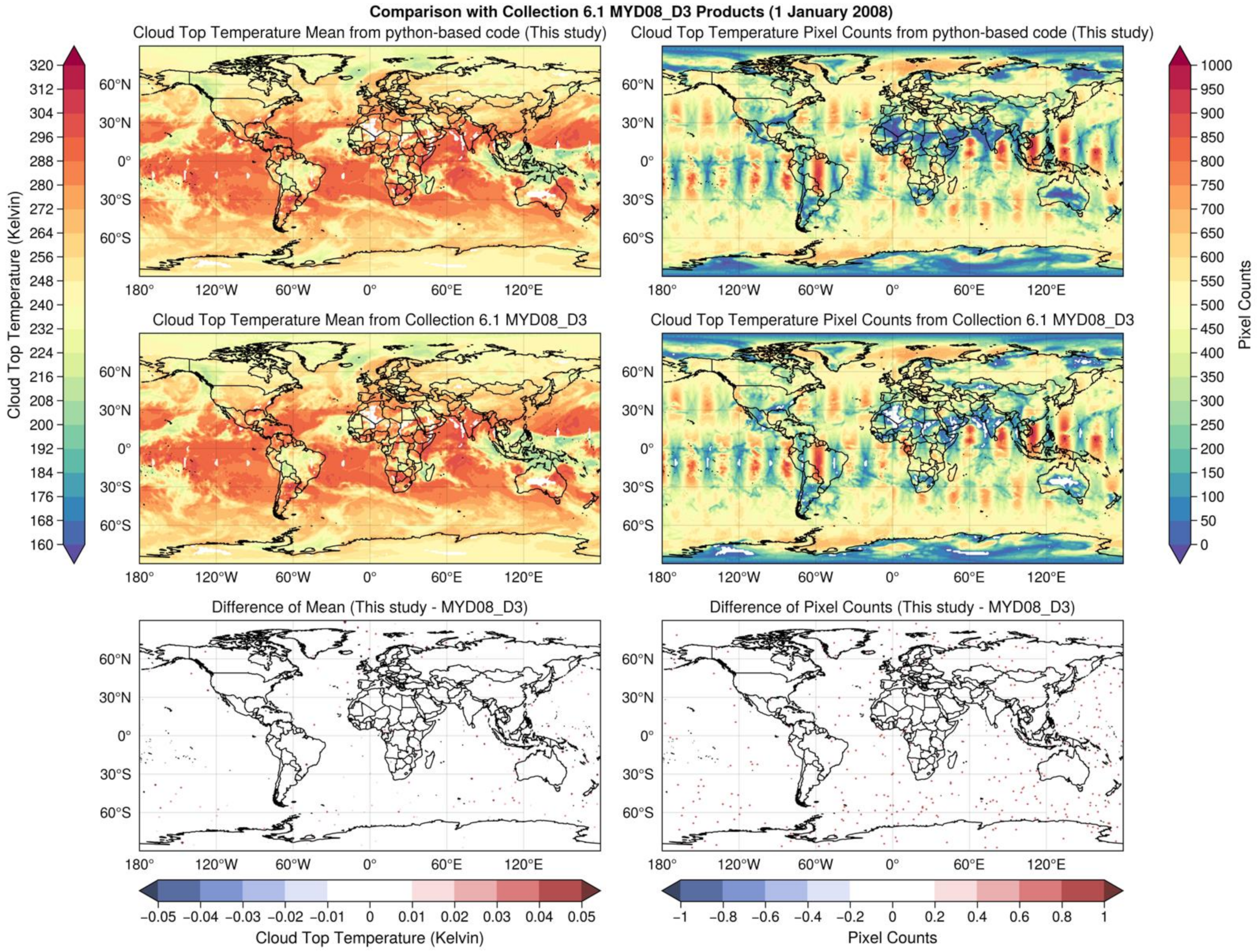
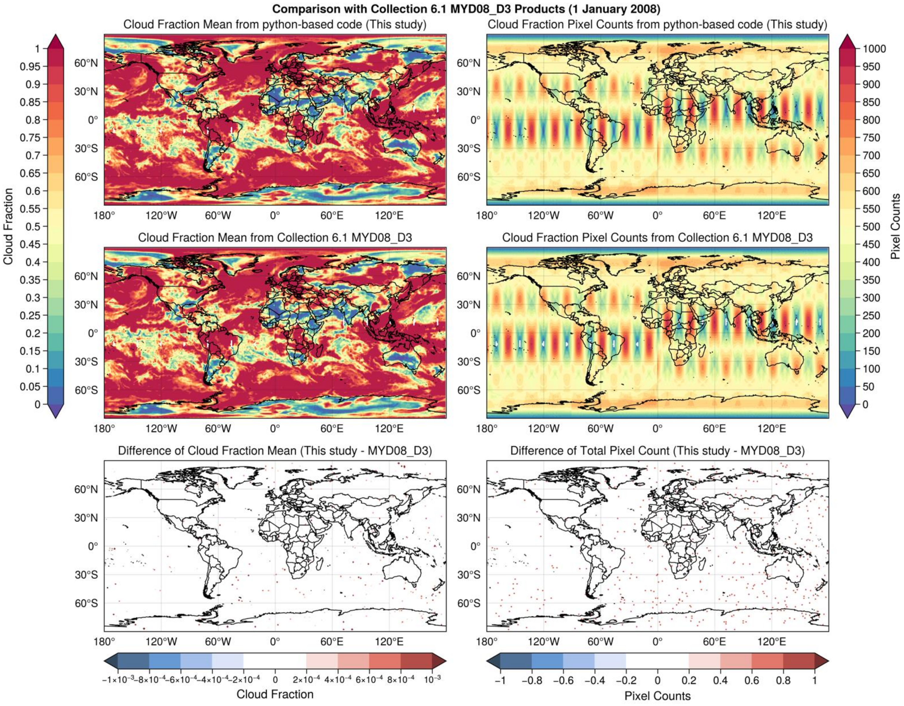
3.1. Comparison with Level-3 MODIS Cloud Product in Collection 6.1 (MYD08_D3)

The straightforward way to validate the aggregation result is to compare the result with the newest version of MODIS L3 products. In this section, we compare the five statistics (i.e., Mean, Pixel Counts, Minimum, Maximum and Standard Deviation) of the cloud top temperature and the cloud fraction with that from the Collection 6.1 Aqua MODIS L3 daily cloud product (MYD08_D3) on 1 January 2008.

According to the user’s guide and ATBD of MODIS atmosphere L3 Product [9], the statistics of cloud top properties and cloud fraction are computed based on the 5-km L2 cloud top properties and cloud fraction from the Collection 6.1 MOD06/MYD06 product. In the L2 MOD06/MYD06 Product [8], the variables at 5 km resolution are averaged by the 5 × 5 1-km L1B input pixels. For example, a 5 km cloud fraction is calculated based on the fraction of cloudy pixels to the total pixels identified by the native 1 km Cloud Mask Flags (see Table 5 in Hubanks, et al. [9]) within the corresponding 5 × 5 km retrieval box.

It is reasonable to aggregate the 5 km L2 cloud fraction instead of computing the fraction of 1 km cloudy pixels, as it is computationally efficient. To be consistent with the MYD08_D3 product, in this section, we choose the 5 km cloud top temperature and th e 5km cloud fraction from the MYD06 product at the input value. The input settings are listed in

Table 2. The inputs that are defined for the direct comparison with MYD08_D3 product on 1 January 2008.

User-Defined Input	Input Value
Range of time	1 January 2008 to 1 January 2008
Regional Boundaries	−90° N~90° N; 180° W~180° E
Spatial resolution	1° by 1°
Sampling rates	1
Statistics	Mean, Pixel Counts, Minimum, Maximum, Standard Deviation
Input variables for aggregation	5 km Cloud Top Temperature and 5 km Cloud Fraction

. However, for a flexible spatial scale, the best quality of the aggregation is to use the native 1 km pixels from the L2 product. As a result, other than the direct comparison with the MYD08_D3 product, the default L3 cloud fraction in our algorithm is obtained directly by calculating the fraction of cloudy pixels identified by the native 1 km Cloud Mask Flags to the total pixel counts within each 1° × 1° degree grid box.

Figure 3 compares the global distribution of the mean value and the pixel counts of the cloud top temperature from our python-based flexible aggregation result with that from the MYD08_D3 product. In addition,

Table 3. The globally averaged differences of the statistics of cloud fraction and cloud top temperatures between the python-based flexible aggregation and the MYD08_D3 product on 1 January 2008.

Variable	Statistics	Difference (This Study—MYD08_D3)	$\mathbf{Percentage}\mathbf{of}\mathbf{Grids}\mathbf{with}\mathbf{Absolute}\mathbf{Difference}<1\times {10}^{-4}$
Cloud Fraction	Minimum	$2.26\times {10}^{-6}$	97.7%
	Maximum	$-2.59\times {10}^{-6}$	99.5%
	Pixel Counts	$-1.54\times {10}^{-5}$	98.6%
	Mean	$4.33\times {10}^{-5}$	98.6%
	Standard Deviation	$4.95\times {10}^{-5}$	98.9%
Cloud Top Temperature	Minimum	$4.10\times {10}^{-4}$	96.5%
	Maximum	$1.22\times {10}^{-3}$	87.4%
	Pixel Counts	$-1.56\times {10}^{-5}$	98.9%
	Mean	$3.44\times {10}^{-5}$	97.3%
	Standard Deviation	$3.08\times {10}^{-5}$	99.2%

lists the globally averaged absolute difference of each of five statistics and the percentage of the number of 1° × 1° grids with an absolute difference less than 1 × 10⁻⁴. For absolute difference within 1 × 10⁻⁴, it can be considered as zero by ignoring the numerical errors due to computational precision. In Figure 3, the results from the python-based flexible aggregation over most of regions (97.3%; see Table 3) match exactly (absolute difference < 1 × 10⁻⁴) with the MYD08_D3. However, there are still some grids that are randomly distributed globally which have slight differences in both the pixel counts (~1 count difference in each grid box) and the mean value (~0.03 Kelvin). These residual differences are possibly due to the reprocessed input L2 granules after the generation of L3 products in the collection 6.1 algorithm from LAADS. As the globally averaged differences of all five statistics (see Table 3) is close to zero (ranging from 1 × 10⁻⁵ to 1 × 10⁻³), we believe that these errors have a negligible impact on the accuracy of the aggregation result.

Figure 4 shows the difference in the mean and pixel counts of the cloud fraction between the two products. The cloud fraction pixel counts represent the total collected pixels from the input L2 granules. As we use the 5 km cloud fraction to compute the mean daily cloud fraction, the difference of the mean value and the pixel counts are within $\pm 0.01$ and within $\pm 1$ pixel counts, respectively (see Figure 4 and Table 3). The mean cloud fraction over most of the regions (98.6%; see Table 3) is well-matched (absolute difference < 1 × 10⁻⁴) with the MYD08_D3. However, users should notice that the cloud fraction computed by the fraction of 1 km cloudy pixels within each grid box is not supposed to be identical with the cloud fraction in the MOD08/MYD08 products. In our algorithm, although users are allowed to choose the MOD06/MYD06 5 km cloud fraction as the input for the L3 cloud fraction, we recommend using the mandatory L3 cloud fraction computed based on the 1 km cloud mask flags if users request a finer spatiotemporal resolution. In summary, the well-matched aggregation result with the L3 product demonstrates the accuracy of the flexible aggregation.

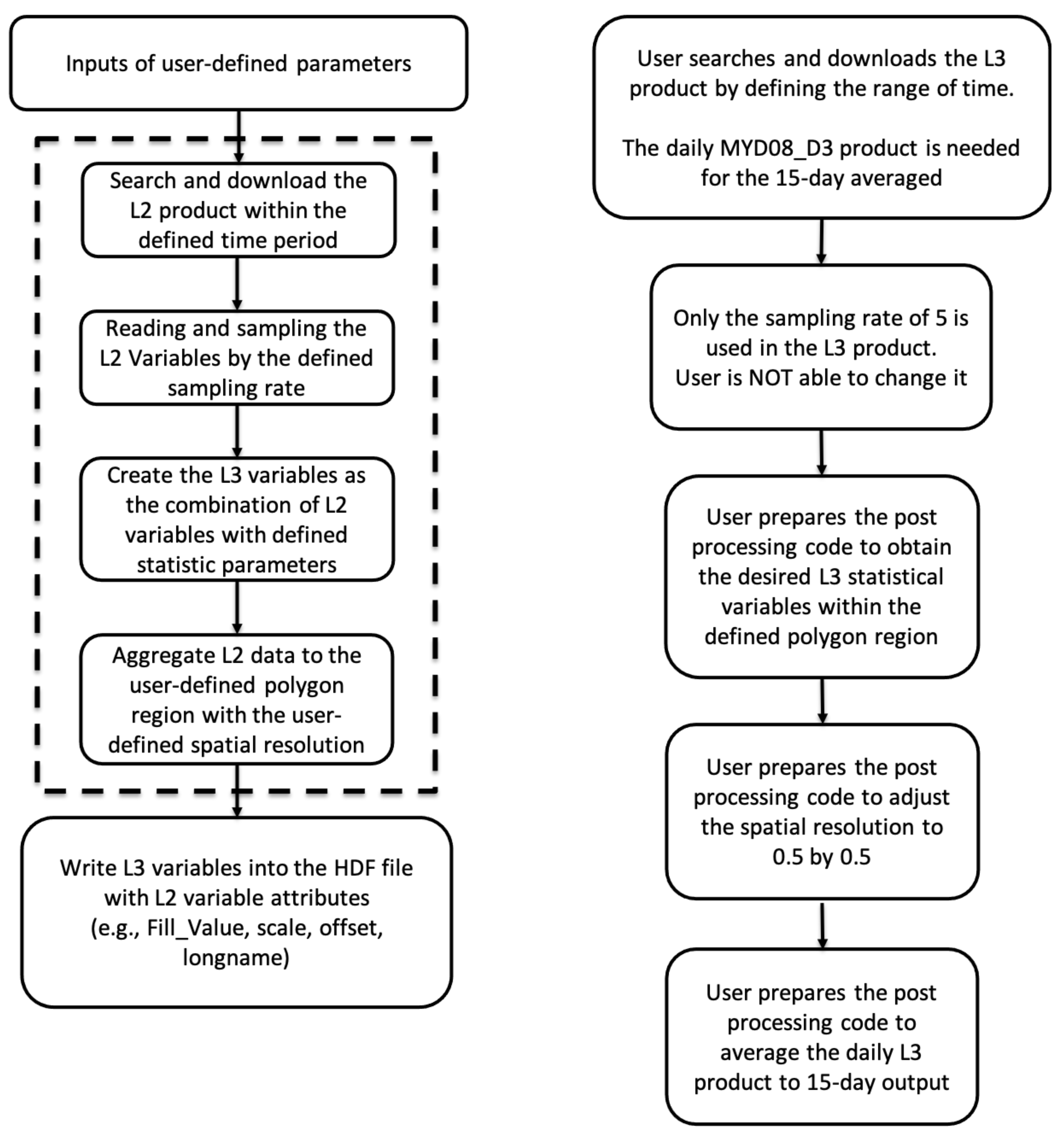
3.2. Comparison of Usage Difference of L3 Data and Flexible Aggregation

After the validation of the aggregation result, in this section, we present the difference of conducting the 15-day averaged cloud top temperature over the northeast Pacific Ocean by using the current L3 products and the flexible aggregation framework.

Table 4. The inputs defined for the 15-day averaged cloud top temperature over the North-East Pacific Ocean.

User-Defined Input	Input Value
Range of time	1 January 2008 to 1 January 2008
Regional Boundaries	20° N~40° N; 120° E~150° E
Spatial resolution	0.5° by 0.5°
Sampling rates	1
Statistics	All seven statistics
Input variables for aggregation	1 km Cloud Top Temperature

lists the required aggregation inputs for this case. It aims to demonstrate three advantages of flexible aggregation compared with leveraging the current L3 MODIS products, which are listed below.

First of all, this aggregation framework helps to get the most targeted dataset that the user needs without operating any post-processing method. For example, if the user needs the MODIS product for a specific range of time within a particular geolocation area. The user has to download the MODIS L3 product and then write codes to derive the targeted data with the desired spatiotemporal resolution. This would require much more effort than simply using the flexible aggregation framework for the targeted dataset.

Secondly, although the recent L3 MODIS product already has around 1000 SDSs, it is still limited regarding all possible combinations of seven statistics with the 127 L2 variables. The flexible aggregation is possible for deriving any combination of the statistics and the L2 variables. Specifically, our approach can maximally generate 762 (127 × 6) statistical SDSs based on single L2 variables for the first six statistics and C (127,2) = 8001 SDSs based on the combination of two L2 variables for the joint 2D histogram, although some of the combinations may not be scientifically meaningful. In other words, if users aim to obtain a statistical SDS that does not exist in the current L3 product but can be found from the L2 variables, the flexible aggregation is capable of achieving it.

Thirdly, instead of downloading the L3 data for the post-processing, users can use the flexible aggregation to directly process the desired dataset on a server (such as a cluster with many compute nodes) using our proposed service (see Section 2.3). The service can download the required L2 data for aggregation automatically at the server. This could save space and time from searching and downloading the L3 data from the data repository.

By using the current L3 product, users have no way but to develop a post-processing code to address the inconsistency with the desired L3 output, including the difference of spatiotemporal resolution, and the sampling rates. Moreover, the downloaded L3 product also requires storage space from the user side. In this case, the daily L3 product for 15 days takes ~3 GB, while the flexible aggregation output only takes ~100 MB for the selected variables and statistics as the flexible aggregation framework only requires users for the defined inputs to generate the L3 output. Figure 5 shows the flow chart of conducting the desired result by using the two different methods. From the flexible aggregation side, the user only needs to take efforts in defining the inputs as the following steps are operated internally. From the side of using the current L3 product, the user’s post-processing code must be able to handle the time average, the interpolation of grids with sub-resolution (i.e., 0.5° by 0.5° grid), and the rectangle region extraction. Therefore, using the flexible aggregation method is more time-saving and space-saving compared with using the current L3 product.

However, it is necessary to point out that the processing time of our aggregation increases with the requested number of files regarding the range of time. It is possible to have a longer processing time using our aggregation method than downloading the current L3 product. To overcome this shortage, we further apply two different scalable approaches (see Section 2.2) to evaluate the speed-up of our aggregation process, which is presented in the next section.

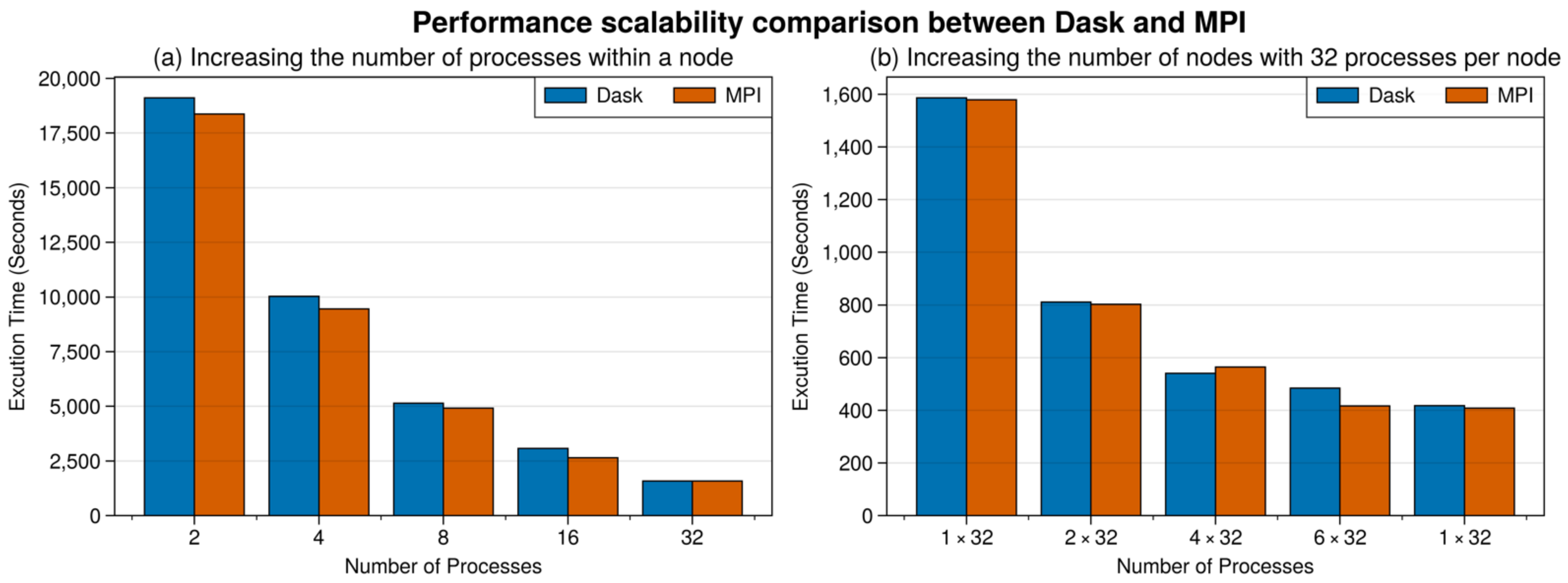
3.3. Speed-Up Improvement of the Parallelization

In this section, we explain the experiments we conducted to benchmark and evaluate the differences of using different parallel platforms. We chose five variables from Aqua MODIS Collection 6.1 L2 cloud product (MYD06) associated with L2 geolocation fields (MYD03) in January 2008 as our aggregation inputs. The inputs are listed in

Table 5. The inputs defined for the Speed-up evaluation.

User-Defined Input	Input Value
Range of time	1 January 2008 to 31 January 2008
Regional Boundaries	−90° N~90° N; 180° W~180° E
Spatial resolution	1° by 1°
Sampling rates	5
Statistics	All seven statistics
Input variables for aggregation	1 km Cloud Top Temperature, 1 km Cloud Top Pressure, 1 km Cloud Top Height, 1 km Cloud Emissivity and 1 km Cloud Mask Flag

. In one month, each of the MYD06 and MYD03 products has 8928 files, with a total data size of 738 GB. The files are located on a centralized data node and are accessed via a network file system (NFS). For software, we used Python (version 3.6.8), Dask (version 1.1.4) and MPI (version 1.4.1).

All experiments were done in a local High-Performance Computing (HPC) cluster. Each computer node has two 16-core Intel Xeon Gold 6140 Skylake CPUs (36 cores in total) and 384 GB of memory. To make a fair comparison, we allocate 2 CPU cores and 20 GB of memory for each parallel process. By running on 1, 2, 4, 6 and 8 nodes, we can have 32, 64, 128, 192 and 256 parallel processes respectively. For Dask execution, we use Slurm [39] to initiate one additional node as the scheduler of distributed jobs, before calling Dask’s scale function to start up the worker nodes to execute the jobs.

We show the execution and speedup results for scalability evaluations of Dask and an MPI-based parallel approach in

Table 6. Execution time (in seconds) and speedup results for scalability evaluation. The serial execution of the one-month data aggregation takes 36,162 s, which serves as a baseline to calculate the speedup of our parallel approaches with Dask and MPI.

Num of Nodes	Num of Processes	Dask Execution Time	Dask Speedup	MPI Execution Time	MPI Speedup
1	2	19,105	1.89	18,368	1.97
1	4	10,036	3.60	9459	3.82
1	8	5143	7.03	4919	7.35
1	16	3076	11.75	2646	13.67
1	32	1586	22.80	1579	22.90
2	64	811	44.59	803	45.03
4	128	540	66.97	564	64.12
6	192	484	74.71	416	86.93
8	256	418	86.50	408	88.63

and Figure 6. In Table 6, we see that the speedup increases almost linearly with the number of processes in execution and reaches up to 86.50 speedups in Dask and 88.63 speedups compared to the serial execution. We also demonstrate the scaling up of the execution time of Dask and MPI in Figure 6a, by increasing the number of processes from 2 to 32 within one computation node. It shows how the execution times decrease proportionally with the increase of the processes and demonstrate how the parallelization improves the data aggregation in both Dask and MPI. We also listed the exact scaling out of execution times of the two parallelization approaches by increasing the number of nodes (each node has 32 processes), as shown in Figure 6b. It shows the execution times of Dask and MPI decrease with the increase of the computing nodes from 1 to 8 nodes, especially the time almost proportionally decrease by increasing 1 computing node to 2 nodes, which demonstrates the parallelization help improves speed up the data aggregation. When scaling up to more nodes such as 6 or 8 nodes, the execution time slightly improves, we believe the overhead of communications increases when more nodes and processes are involved. For the comparison between MPI and Dask, the speedups done via MPI are better than those via Dask in most cases. We think this is due to less coordination overhead for MPI-based parallelization. It shows the advantage of MPI because of its low coordination overhead, especially if the static scheduling via the MPI approach happens to achieve relatively balanced workloads among different nodes.

4. Summaries and Conclusions

While the development of remote sensing techniques greatly improves our understanding of the Earth, it also brings two challenges. First, the ever-increasing volume of the available remote sensing observation data is difficult to download and process. Second, the current static and “one-size-fits-all” data provision method by most remote sensing data providers such as NASA DAACs is difficult to meet increasing diverse usage requirements from the community. To address these two challenges, we propose a service-oriented flexible and efficient MODIS aggregation framework. Using this framework, users only need to get an aggregated MODIS L3 data based on their unique requirements and the aggregation can run in parallel to achieve speedup. The experiments show that our aggregation results are almost identical to the current MODIS L3 products and our parallel execution with 256 processes (8 computing nodes) in total can be 88.63 times faster than a serial code execution on the single node.

Our work is an open source at a GitHub repository [40] via link https://github.com/big-data-lab-umbc/MODIS_Aggregation (accessed on 3 September 2021). The installation document of our library and some usage examples of our algorithm are shown in the GitHub repository. The examples mainly demonstrate how to conduct local execution, a Dask-based distributed execution and an MPI-based distributed execution. All these three execution modes invoke the same functions implemented by our library. Besides these core usage examples, we also show examples for a result comparison and service-based deployment.

Because commercial cloud computing providers such as Amazon Web Services (AWS) [41] provide both service-oriented architecture and an on-demand distributed computing environment, our work can be easily extended to work with these environments. We believe our work shows promising opportunities for many other climate data analytics applications.

It is necessary to admit that there are still limitations in our aggregation framework. First of all, the current version of our algorithm does not support L3 outputs with regular daily, 8-day and monthly temporal resolutions within the defined range of time, as the temporal resolution is defined in a flexible way to cover different time ranges. Secondly, the current version has not yet been capable of replicating all L3 statistics from Collection 6/6.1 MOD08/MYD08 products, especially for those where the L2 runtime QA information is needed for physical property-based aggregation. For instance, the cloud optical properties that are classified regarding different cloud phases (i.e., liquid, ice and mixed) in L3 products have an additional dependency on the cloud retrieval phase flag in the runtime QA flag from the MOD06/MYD06 product. Our algorithm does not support the additional combinations of L3 statistics on these variables. Accordingly, the current version of the algorithm is not able to handle the various requests of quality control on the input L2 data either. The improvements could be achieved in future developments. However, since our algorithm is openly accessible on GitHub, it is convenient for users to extend the input preprocessing module of our algorithm to meet the requirement of their L2 input quality control.

References

1. Salomonson, V.V.; Barnes, W.; Xiong, J.; Kempler, S.; Masuoka, E. An overview of the Earth Observing System MODIS instrument and associated data systems performance. In Proceedings of the IEEE International Geoscience and Remote Sensing Symposium, Toronto, ON, Canada, 24–28 June 2002; pp. 1174–1176. [Google Scholar]
2. Lee, J.; Kim, J.; Yang, P.; Hsu, N.C. Improvement of aerosol optical depth retrieval from MODIS spectral reflectance over the global ocean using new aerosol models archived from AERONET inversion data and tri-axial ellipsoidal dust database. Atmos. Chem. Phys. 2012, 12, 7087–7102. [Google Scholar] [CrossRef] [Green Version]
3. Xiong, X.; Chiang, K.; Esposito, J.; Guenther, B.; Barnes, W. MODIS on-orbit calibration and characterization. Metrologia 2003, 40, S89. [Google Scholar] [CrossRef]
4. Justice, C.; Townshend, J.; Vermote, E.; Masuoka, E.; Wolfe, R.; Saleous, N.; Roy, D.; Morisette, J. An overview of MODIS Land data processing and product status. Remote Sens. Environ. 2002, 83, 3–15. [Google Scholar] [CrossRef]
5. Huete, A.; Didan, K.; Miura, T.; Rodriguez, E.P.; Gao, X.; Ferreira, L.G. Overview of the radiometric and biophysical performance of the MODIS vegetation indices. Remote Sens. Environ. 2002, 83, 195–213. [Google Scholar] [CrossRef]
6. Righi, M.; Andela, B.; Eyring, V.; Lauer, A.; Predoi, V.; Schlund, M.; Vegas-Regidor, J.; Bock, L.; Brötz, B.; de Mora, L. Earth System Model Evaluation Tool (ESMValTool) v2. 0–technical overview. Geosci. Model Dev. 2020, 13, 1179–1199. [Google Scholar] [CrossRef] [Green Version]
7. Masuoka, E.; Fleig, A.; Wolfe, R.E.; Patt, F. Key characteristics of MODIS data products. IEEE Trans. Geosci. Remote 1998, 36, 1313–1323. [Google Scholar] [CrossRef]
8. Platnick, S.; King, M.D.; Meyer, K.G.; Wind, G.; Amarasinghe, N.; Marchant, B.; Arnold, G.T.; Zhang, Z.; Hubanks, P.A.; Ridgway, B.; et al. MODIS Cloud Optical Properties: User Guide for the Collection 6/6.1 Level-2 MOD06/MYD06 Product and Associated Level-3 Datasets. Version 2018, 1, 150. [Google Scholar]
9. Hubanks, P.A.; Platnick, S.; King, M.D.; Ridgway, B. MODIS Atmosphere L3 Global Gridded Product User’s Guide & algorithm theoretical basis document (ATBD) for C6.1 products: 08_D3, 08_E3, 08_M3. Version 2020, 1, 129. [Google Scholar]
10. Savtchenko, A.; Ouzounov, D.; Ahmad, S.; Acker, J.; Leptoukh, G.; Koziana, J.; Nickless, D. Terra and Aqua MODIS products available from NASA GES DAAC. Adv. Space Res. 2004, 34, 710–714. [Google Scholar] [CrossRef]
11. Park, S.S.; Kim, J.; Lee, J.; Lee, S.; Kim, J.S.; Chang, L.S.; Ou, S. Combined dust detection algorithm by using MODIS infrared channels over East Asia. Remote Sens. Environ. 2014, 141, 24–39. [Google Scholar] [CrossRef] [Green Version]
12. Zhang, P.; Lu, N.-M.; Hu, X.-Q.; Dong, C.-H. Identification and physical retrieval of dust storm using three MODIS thermal IR channels. Glob. Planet Chang. 2006, 52, 197–206. [Google Scholar] [CrossRef]
13. Platnick, S.; Heidinger, A.; Ackerman, S.; Amarasinghe, N.; Dutcher, S.; Frey, R.; Hubanks, P.; Li, Y.; Marchant, B.; Meyer, K. EOS MODIS and SNPP VIIRS Cloud Properties: User Guide for the Climate Data Record Continuity Level-2 Cloud Top and Optical Properties Product (CLDPROP); Technical Report; NASA Goddard Space Flight Center: Greenbelt, MD, USA, 2019.
14. Ruiz-Arias, J.; Dudhia, J.; Gueymard, C.; Pozo-Vázquez, D. Assessment of the Level-3 MODIS daily aerosol optical depth in the context of surface solar radiation and numerical weather modeling. Atmos. Chem. Phys. 2013, 13, 675–692. [Google Scholar] [CrossRef] [Green Version]
15. NASA LAADS Distributed Active Archive Center. Available online: https://ladsweb.modaps.eosdis.nasa.gov/search/ (accessed on 30 June 2021).
16. Acker, J.G.; Leptoukh, G. Online analysis enhances use of NASA earth science data. Eos Trans. Am. Geophys. Union 2007, 88, 14–17. [Google Scholar] [CrossRef]
17. Wang, J.; Huang, X.; Zheng, J.; Rajapakshe, C.; Kay, S.; Kandoor, L.; Maxwell, T.; Zhang, Z. Scalable Aggregation Service for Satellite Remote Sensing Data. In Proceedings of the International Conference on Algorithms and Architectures for Parallel Processing, New York, NY, USA, 2–4 October 2020; pp. 184–199. [Google Scholar]
18. Chang, I.; Gao, L.; Burton, S.P.; Chen, H.; Diamond, M.S.; Ferrare, R.A.; Flynn, C.J.; Kacenelenbogen, M.; LeBlanc, S.E.; Meyer, K.G.; et al. Spatiotemporal Heterogeneity of Aerosol and Cloud Properties Over the Southeast Atlantic: An Observational Analysis. Geophys. Res. Lett. 2021, 48, e2020GL091469. [Google Scholar] [CrossRef]
19. Cai, Y.; Guan, K.; Lobell, D.; Potgieter, A.B.; Wang, S.; Peng, J.; Xu, T.; Asseng, S.; Zhang, Y.; You, L.; et al. Integrating satellite and climate data to predict wheat yield in Australia using machine learning approaches. Agric. For. Meteorol. 2019, 274, 144–159. [Google Scholar] [CrossRef]
20. Hubanks, P.A. MODIS Atmosphere QA Plan for Collection 061. Version 2017, 1, 67. [Google Scholar]
21. Sayer, A.M.; Knobelspiesse, K.D. How should we aggregate data? Methods accounting for the numerical distributions, with an assessment of aerosol optical depth. Atmos. Chem. Phys. 2019, 19, 15023–15048. [Google Scholar] [CrossRef] [Green Version]
22. Levy, R.C.; Leptoukh, G.G.; Kahn, R.; Zubko, V.; Gopalan, A.; Remer, L.A. A critical look at deriving monthly aerosol optical depth from satellite data. IEEE T. Geosci. Remote 2009, 47, 2942–2956. [Google Scholar] [CrossRef]
23. Colarco, P.R.; Kahn, R.A.; Remer, L.A.; Levy, R.C. Impact of satellite viewing-swath width on global and regional aerosol optical thickness statistics and trends. Atmos. Meas. Tech. 2014, 7, 2313–2335. [Google Scholar] [CrossRef] [Green Version]
24. Li, R.; Hu, H.; Li, H.; Wu, Y.; Yang, J. MapReduce parallel programming model: A state-of-the-art survey. Int. J. Parallel Program. 2016, 44, 832–866. [Google Scholar] [CrossRef]
25. Maitrey, S.; Jha, C. MapReduce: Simplified data analysis of big data. Procedia Comput. Sci. 2015, 57, 563–571. [Google Scholar] [CrossRef] [Green Version]
26. Dean, J.; Ghemawat, S. Mapreduce: Simplified data processing on large clusters. Commun. ACM 2008, 51, 107–113. [Google Scholar] [CrossRef]
27. Rocklin, M. Dask: Parallel computation with blocked algorithms and task scheduling. In Proceedings of the 14th Python in Science Conference, Austin, TX, USA, 6–12 July 2015; p. 136. [Google Scholar]
28. Pacheco, P. Parallel Programming with MPI; Morgan Kaufmann: Burlington, MA, USA, 1997. [Google Scholar]
29. Dalcín, L.; Paz, R.; Storti, M. MPI for Python. J. Parallel Distrib. Comput. 2005, 65, 1108–1115. [Google Scholar] [CrossRef]
30. Perrey, R.; Lycett, M. Service-oriented architecture. In Proceedings of the 2003 Symposium on Applications and the Internet Workshops, Orlando, FL, USA, 27–31 January 2003; pp. 116–119. [Google Scholar]
31. Laskey, B.; Laskey, K. Service oriented architecture. Wiley Interdiscip. Rev. Comput. Stat. 2009, 1, 101–105. [Google Scholar] [CrossRef]
32. Schnase, J.L. Climate analytics as a service. In Cloud Computing in Ocean and Atmospheric Sciences; Elsevier: Amsterdam, The Netherlands, 2016; pp. 187–219. [Google Scholar]
33. Stratus: Synchronization Technology Relating Analytic Transparently Unified Services. Available online: https://github.com/nasa-nccs-cds/stratus/ (accessed on 30 June 2021).
34. Hintjens, P. ZeroMQ: Messaging for Many Applications; O’Reilly Media Inc.: Newton, MA, USA, 2013. [Google Scholar]
35. Fengping, P.; Jianzheng, C. Distributed system based on ZeroMQ. Electron. Test 2012, 7, 24–29. [Google Scholar]
36. ZeroMQ: An Open-Source Universal Messaging Library. Available online: https://zeromq.org/ (accessed on 30 June 2021).
37. OpenAPI Initiative (OAI). Available online: www.openapis.org (accessed on 30 June 2021).
38. Pautasso, C.; Wilde, E.; Alarcon, R. REST: Advanced Research Topics and Practical Applications; Springer: Berlin/Heidelberg, Germany, 2013. [Google Scholar]
39. Slurm Workload Manager. Available online: https://slurm.schedmd.com/overview.html (accessed on 30 June 2021).
40. Scalable MODIS Data Aggregation Platform. Available online: https://github.com/big-data-lab-umbc/MODIS_Aggregation (accessed on 30 June 2021).
41. Amazon Web Services (AWS). Available online: https://aws.amazon.com (accessed on 30 June 2021).
Figure 1. Illustration of data partitioning-based parallel aggregation with one-month data.
Remotesensing 13 03541 g001
Figure 2. Integration of Stratus service framework with parallel MODIS aggregation.
Remotesensing 13 03541 g002
Figure 3. The comparison of the mean value and pixel counts of cloud top temperature between the python-based flexible aggregation algorithm and the MYD08_D3 product on 1 January 2008.
Remotesensing 13 03541 g003
Figure 4. The comparison of the cloud fraction between the python-based algorithm and the MYD08_D3 product on 1 January 2008.
Remotesensing 13 03541 g004
Figure 5. The flow chart of the aggregation on the desired cloud top temperature by using the flexible aggregation framework (left) and the current L3 product (right). The dashed box indicates the internal process in the python-based flexible aggregation method.
Remotesensing 13 03541 g005
Figure 6. Execution time results (in seconds) for scalability evaluation by (a) increasing the number of processes within a node and (b) increasing the number of nodes with 32 processes per node.
Remotesensing 13 03541 g006